MTH5: an archive and exchangeable data format for magnetotelluric time series data

Abstract

Magnetotellurics (MT) is a passive electromagnetic geophysical method that measures variations in subsurface electrical resistivity. MT data are collected in the time domain and processed in the frequency domain to produce estimates of a transfer function representing the Earth’s electrical structure. Unfortunately, the MT community lacks metadata and data standards for time series data. As the community grows and findability, accessibility, interoperability, and reuse of digital assets (FAIR) data principles are enforced by government and funding agencies, a standard is needed for time series data. Presented here is a hierarchical data format (MTH5) that is logically formatted to how MT data are collected. Open-source Python packages are also described to read, write, and manipulate MTH5 files. These include a package to deal with metadata (mt_metadata) based on standards developed by the Working Group for Magnetotelluric Data Handling and Software assembled by the Incorporated Research Institutions for Seismology (IRIS), and mth5: a package to interact with MTH5 files that uses mt_metadata. Example code and workflows are presented.

1 Introduction

Magnetotellurics (MT) is an electromagnetic geophysical method that is sensitive to variations in subsurface electrical resistivity (Chave and Jones, 2012). MT measurements are useful for imaging various geologic systems, including geothermal (e.g. Peacock et al. (2020)), mineral (e.g. Heinson et al. (2018)), volcanic (e.g. Bedrosian et al. (2018)), subduction (e.g. Cordell et al. (2019)), seismic (e.g. Karaş et al. (2020)), and geomagnetic hazards (e.g. Kelbert (2019); Murphy et al. (2021)). Physically, MT utilizes Faraday’s law of electromagnetic induction, where the Earth’s magnetic field varies temporally in response to interactions of solar wind with natural magnetospheric and ionspheric current systems, inducing electric fields in the conducting Earth. Magnetic fields are assumed to be horizontally polarized and impinge on the Earth’s surface at normal incidence. At the surface these magnetic fields diffuse into the Earth inducing electric fields. A vertical magnetic field can be induced by subsurface horizontal electrical currents. Field measurements are collected in the time domain measuring two horizontal orthogonal electric fields, two horizontal orthogonal magnetic fields, and often a vertical magnetic field. Subsurface electrical resistivity is estimated by transforming the time domain electromagnetic fields into the frequency domain and calculating a frequency dependent transfer function (Egbert, 2002; Chave and Thomson, 2004). This transfer function describes how the Earth’s electrical structure transforms time varying magnetic fields into time varying electric fields.

The principles of findability, accessibility, interoperability, and reuse of digital assets (FAIR) has become standard for many institutions (Wilkinson et al., 2016), as such the need for metadata and data structure standards is imperative. Unfortunately, the MT community does not have a standard for time series observations and datasets. The international MT community has traditionally been small compared to other geophysics research communities such as seismology, and MT groups are usually small clusters that have internally developed workflows to organize time series and estimate transfer functions. Sharing of the raw MT data (time series) or the processed MT data (transfer functions) has not, historically, been a priority in the MT community (Kelbert et al., 2018) due to the heterogeneity of data formats and the lack of incentives for sharing. However, the broadening of applications for MT data and increase in the adherence to FAIR principles by government and academic institutions leads us to pursue a standard format for containing MT time series data and metadata, to complement a FAIR data solution recently completed for MT transfer functions (Kelbert et al., 2011; Kelbert, 2020).

As part of the Seismological Facility for the Advancement of Geoscience (SAGE) facility (https://www.nsf.gov/awardsearch/showAward?AWD_ID=1851048), an National Science Foundation (NSF) sponsored effort to establish new MT science capabilities for principal investigators (PIs), the Incorporated Research Institutions for Seismology (IRIS) established a Working Group in 2019 for Magnetotelluric Data Handling and Software (https://www.iris.edu/hq/about_iris/governance/mt_soft). This group consisted of MT experts and IRIS staff, who were charged with defining a metadata standard and data format that would be used by the new MT instruments operated through IRIS, as well as support interoperability in a discipline-specific manner. The working group met remotely over two-dozen times (roughly an hour each) between spring 2019 and fall 2020 to devise, refine, and implement a framework to describe and store MT time series. This paper presents open-source Python tools to read and write the agreed upon metadata standards Peacock et al. (2021) and data format. Here we will describe the time series metadata, discuss the open-source Python package mt_metadata, and introduce the data container and open-source Python package MTH5. All examples code in this manuscript, and more, are available as working Jupyter Notebooks in a zero-install environment using mybinder.org. The links are found on the GitHub landing page of each repository website by clicking the Binding badge, or follow these links for mt_metadata: https://mybinder.org/v2/gh/kujaku11/mt_metadata/main and mth5: https://mybinder.org/v2/gh/kujaku11/mth5/master.

2 Time Series Metadata

2.1 Metadata Description

Development of time series metadata involved detailed discussion of metadata keywords, meanings, and hierarchy both within the group and with the wider MT community. To frame this approach, the group leveraged other metadata standards (e.g. Climate Forecasting (Hassell et al. 2017), International Federation of Digital Seismograph Networks (FDSN; https://www.fdsn.org), International Organization for Standardization (ISO; https://www.iso.org/home.html)). Community input on the MT-specific metadata details was sought through multiple outreach efforts over the course of several years of development. Each metadata keyword is defined by 8 attributes and an example attribute (Table 1). The complete specification of the MT time series metadata standards can be found in Peacock et al. (2021).

Table 1: Metadata attributes

Attribute	Description
Name	A full descriptive name that is logical for the keyword. Forced to be all lower case and full words separated by _
Type	Base data type [ string | float | int | Boolean ]
Style	Describes how the string should be formatted. Options are included in Table 2
Required	True if required or False if optional
Units	Physical units of the keyword. Given as full name all lowercase separated by _ and a - for multiplicative units (e.g. ohm-meters) and per for a ratio of units (e.g. meters per second)
Description	Detailed description of what the keyword represents
Options	If "style" is "controlled vocabulary" this is a list of accepted options
Example	An example use of the keyword
Default	A default value, only set if Required = True

Table 2: Acceptable String Formats

Style	Description	Example
Free Form	An unregulated string that can contain {a-z, A-Z, 0-9} and special characters	This is Free Form!
Alpha Numeric	A string that contains no spaces and only characters {a-z, A-Z, 0-9, -, _}	WGS84
Controlled Vocabulary	Only certain names or words are allowed. In this case, examples of acceptable values are provided in the documentation as [ option01 $|$ option02 $|$ … ]. The … indicates that other options are possible but have not been defined in the standards yet	reference_frame = geographic
List	List of entries using a comma separator	Ex, Ey, Hx, Hy, Hz, T
Number	A number according to the data type; number of decimal places has not been implemented yet	10.0 (float) or 10 (integer)
Date	ISO formatted date YYYY-MM-DD in UTC	2020-02-02
Date Time	ISO formatted date time YYYY-MM-DDThh:mm:ss.ms+00:00 in UTC	2020-02-02T12:20:45.123456+00:00
Email	A valid email address	person@mt.org
URL	A full URL that a user can view in a web browser	https://www.passcal.nmt.edu/

2.2 Metadata Hierarchy

Metadata keywords are structured to be hierarchical such that more complicated metadata can be represented as a combination of simpler keywords. This is done by combining keywords with a period to create nested keywords, for example to describe the latitude of a location one could use location.latitude.

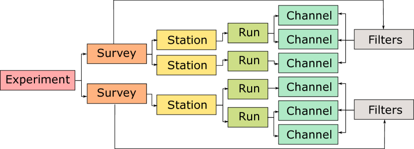
The hierarchy and structure of the MT metadata logically follows how MT time series data are collected (Figure 1). The highest level is an Experiment which contains all metadata for an MT experiment collected in a geographical region. The next level down is Survey which contains metadata for data collected over a certain time interval in a given geographic region. This may include multiple PIs or data collection episodes but should be confined to a specific project. Next level down is a Station which contains metadata for a single location over a certain time interval. Beneath station is the Run level. A Run contains metadata for continuous data collected at a single sample rate. If the station location changes during a run, then a new Station should be created and subsequently a new Run under the new station. If the sensors, cables, data logger, battery, etc. are replaced during a run but the station remains in the same location, then this can be recorded in the Run metadata but does not require a new station. Finally, a Channel contains metadata for a single channel during a single run, where electric, magnetic, and auxiliary channels have specific metadata to uniquely describe the physical measurement. Metadata standards for each level are defined in Peacock et al. (2021). If channel parameters are changed between runs, this would require creating a new run. If a run has channels that drop out, the start and end period will be the minimum time and maximum time for all channels recorded and those channels that dropped will be filled with null values.

A Filters level exists at the Survey level and describes all filters applied to the time series data to get calibrated data in useful physical units. The Filters level is placed here to remove redundancy at the channel level of repeating filter metadata. Currently five different types of filters are supported: frequency-amplitude-phase tables, pole-zero filters, finite impulse response filters, coefficient filters, and time-delay filters. Each channel has two keywords that define the filters and both are lists of the same length: channel.filter.name is a list of filter names to calibrate the data and channel.filter.applied is a list of booleans indicating whether the filter has been applied (true) or not (false). Both of these lists must be ordered the same as how the filters are applied. An applied filter means the data have been transformed in some way, for example calibrating the data from physical units to digital counts.

Figure 1: Example of how MT time series metadata are structured. Top level is an Experiment, then Survey which contains all the filter metadata for the survey as a dictionary keyed by filter name. The next level down is Station, then Run, and finally Channel. The Channel metadata contains the names of filters used and whether they have been applied. To get filter metadata, retrieve the metadata from the filter dictionary stored at the Survey level.

2.3 Formatting Standards

Specific and required formatting standards for location, time and date, and angles are defined to follow international standards and MT conventions.

2.3.1 Time and Date Format

All time and dates are given as an ISO formatted date-time string in the coordinated universal time (UTC) time zone. The ISO date-time format is YYYY-MM-DDThh:mm:ss.ms+00:00, where the UTC time zone is represented by +00:00. UTC can also be denoted by Z at the end of the date-time string YYYY-MM-DDThh:mm:ss.msZ. Note that Z can also represent Greenwich Mean Time (GMT) but is an acceptable representation of UTC time. If the data requires a different time zone, this can be accommodated, however UTC is preferred whenever possible to avoid confusion of local time and local daylight savings. Milliseconds can be accurate to nine decimal places. ISO dates are formatted YYYY-MM-DD, and ISO hours are given as a 24 hour number or military time, e.g. 4:00 AM is 04:00 and 4:00 PM is 16:00.

2.3.2 Location

All latitude and longitude locations are given in decimal degrees in the datum specified at the Survey level. The datum is static, and should follow the well-known text format described by the Open Geospatial Consortium (Open Geospatial Consortium, 2019), for example WGS84. The entire survey should use only one datum that is specified at the Survey level, therefore the user must project all coordinates to the specified datum. All locations are relative to the prime meridian (0, 0). Latitude values must be within $[-90,90]$, where negative values represent locations south of the prime meridian. Longitude values must be within $[-180,180]$, where negative values are west of the prime meridian. Elevation and other distance values are given in meters. The preferred datum is WGS84 but others are acceptable.

2.3.3 Angles

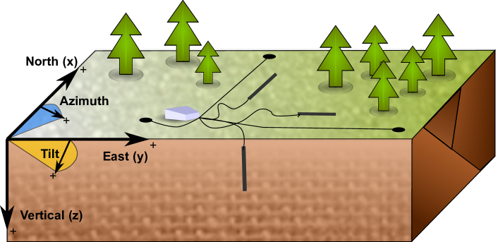
All angles of orientation are given in decimal degrees. Orientation of channels should be given in a geographic or a geomagnetic reference frame where the right-hand coordinates are assumed to be north = 0, east = 90, and vertical is positive downward (Figure 2). The coordinate reference frame is given at the station level
station.orientation.reference_frame. Two angles to describe orientation of a sensor are given by
channel.measurement_azimuth and channel.measurement_tilt. In a geographic or geomagnetic reference frame, the azimuth refers to the horizontal angle relative to north positive clockwise, and the tilt refers to the vertical angle with respect to the horizontal plane. In this reference frame, a tilt angle of 90 points downward, 0 is parallel with the surface, and -90 points upwards.

Archived data should remain in measurement coordinates. Any transformation of coordinates for derived products can be stored in the transformation angles at the channel level in channel.transformed_azimuth and
channel.transformed_tilt, and the transformed reference frame can then be recorded in
station.orientation.transformed_reference_frame.

Figure 2: Diagram showing a right-handed geographic coordinate system. The azimuth is measured positive clockwise along the horizontal axis and tilt is measured from the horizontal axis with positive down = 90, positive up = 180, and horizontal = 0.

2.4 Units

Acceptable units are only those from the International System of Units (SI). Only long names in all lower case are acceptable. Units with multiple dimensions should be separated by a - if multiplicative, or per if divided. For example velocity would be meters per second and resistivity would be ohm-meter.

2.5 Open-source Python package: mt_metadata

To help users handle, validate, and manipulate MT time series metadata, an open-source Python package has been developed: mt_metadata. The base container provides functions to read/write XML, JSON, and Python dictionaries, and validates each metadata keyword and value against attributes described in Section 2.1. This base container is inherited by containers representing each level of MT metadata. All time series metadata objects are included in the mt_metadata.timeseries module.

The internal structure of the base class begins with reading in the metadata standards defined by Peacock et al. (2021), which are stored as JSON files included in the distribution. The standards files are read in as a Python dictionary and stored as a private variable. The keys of this private dictionary are attribute names and values are dictionaries describing the metadata attribute (Table 1). The base class is also assigned attributes that are the key names for the user to access. When the value of a base class attribute is modified, the value is validated against the defined standards in the following order: "name", "data type", "style", and "options" using validation functions for each standard type. If the input data is not the required data type, the data type validator will attempt to convert the value to the required data type. If validation fails at any point, an error is raised. Note that the base class is not limited to MT data, but any standardized metadata following Section 2.1.

The base class provides methods to get information about attributes, add new attributes, get and set attributes, print string representation, read/write XML, JSON, and Python dictionaries, update from a dictionary, and compare similar objects. Example Jupyter Notebook code is provided in Figure 3.

Figure 3: Example code for how to access the attribute list of a metadata class, get a description of an attribute, and how the validators convert input to the appropriate data type. Source code can be found at https://github.com/kujaku11/mt_metadata/tree/main/examples/notebooks/example_01.ipynb

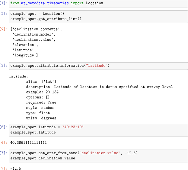
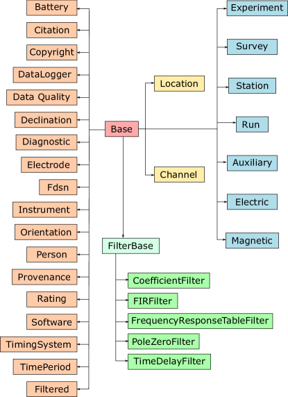
Time series metadata have been broken down into the primitive representation and made into class objects that inherit the base class (Figure 4). These are then used as attributes for more complex objects. For example declination describes how declination was estimated, which can be an attribute of location. The declination value for the given location is then location.declination.value (Figure 3).

Figure 4: Inheritance plot of the Base class for time series metadata objects. Objects on the left are used as attributes from more complex objects on the right. For example "survey.provenance.author". The filters have a base class that inherits the main base class. FIRFilter: finite impulse response filter; FDSN: International Federation of Digital Seismograph Networks.

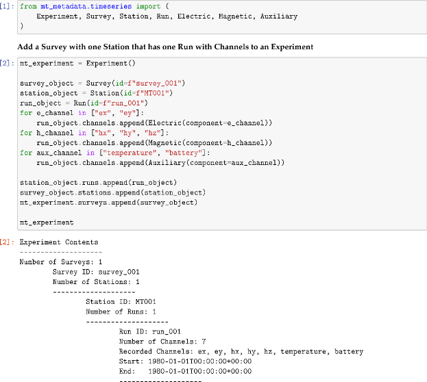
Following the structure displayed in Figure 1, each level container includes an attribute that is a list of the containers for the next level down (Figure 5). For example, Experiment has an attribute Experiment.surveys which is a list of Survey objects. Moreover, Survey has an attribute Survey.stations, which is a list of Station objects, and so on down the chain to Channel. This provides a logical structure of metadata objects and allows for writing and reading comprehensive metadata. More information can be found at https://mt-metadata.readthedocs.io/en/latest/.

Figure 5: Example code of how to make an Experiment metadata object from scratch and examine its contents. Source code can be found at https://github.com/kujaku11/mt_metadata/tree/main/examples/notebooks/example_02.ipynb.

3 MTH5

Several geophysical communities format data in hierarchical data formats like HDF5 and NetCDF-4 because these formats contain data and metadata in the same place for a self describing logically structured data set. HDF and HDF5 files have mutliple benefits (The HDF Group, 2019): 1) the base code is open-source and community driven; 2) files are flexible; 3) file size is only limited by available resources; 4) files are portable across nearly all operating systems and platforms from laptops to cloud based parallel systems, and have no limitations on the number of data objects contained within the file ; 5) RAM requirements are optimized with a high-performance input/output system to only load requested data; 6) chunking and compression are inherent to optimize efficient storage and retrieval. A single writer with multiple readers (SWMR) is supported, but parallel reading/writing needs parallel HDF5 (PHDF5). For cloud environments the HDF Group provides highly scalable data services (HSDS).

Most data collected by satellites are stored as platform specific HDF5 files that provide users with multi-channel map-oriented products (e.g. Lee (2012); Klein and Taaheri (2016); Loomis et al. (2019)). For ground based measurements, an adaptable seismic data format (ASDF) has been developed to store various seismic data with provenance (Krischer et al., 2016). The authors suggest ASDF could be extended to other geophysical data types in the future. IRIS Portable Array Seismic Studies of the Continental Lithosphere (PASSCAL) also developed an HDF5 container the PASSCAL hierarchical format (PH5), which is their contemporary format to archive seismic data for large assembled datasets. We pursued extending ASDF and PH5 but decided to build a specific container for MT data (MTH5) that could potentially be an extension in the future to ASDF, PH5, and the planned geophysical format being developed by IRIS and UNAVCO, which will be a flexible format to store various types of geophysical data (Habermann et al., 2021). MTH5 is an HDF5 file and the open-source Python module mth5 provides tools to interface with the file.

Figure 6: Schematic of the MTH5 file structure. The top group is Experiment which has three subgroups: Surveys, Reports and Standards. The Standards group contains the metadata standards used to make the file and is stored as a table for easy reference. The Reports group can contain any auxiliary reports that compliment or help describe the data. The Surveys group can contain multiple Survey groups. A Survey group contains a Filters group, which has a subgroup for each supported filter (see Figure 4 for supported filters), and contains all filters for a given survey. A Survey group can have multiple Station groups. A Station group can have multiple Run groups. A Run can have multiple Channel data sets which is ultimately where data are stored. Each group and data set includes metadata attributes of the appropriate level. Each Survey, Station, Run group is named by its id, and Channel data sets are named by their component. For example the path to MagneticChannel02 of Survey02 would be Experiment/Survey_02/Station_01/Run_02/Magnetic_Channel_02.

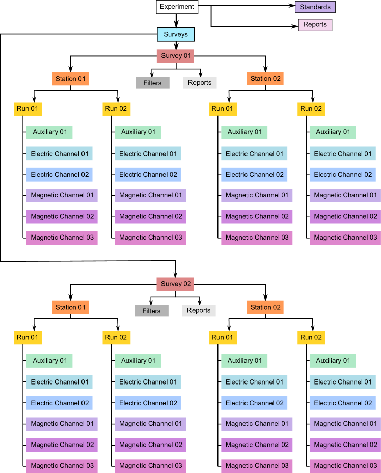
Two main types of structures exist in HDF5 files: groups and data sets. Groups are similar to folders in a filing system but with the ability to store metadata as attributes. Data sets store data and can also have metadata attached. The structure of an MTH5 file follows how MT time series data are collected (Figure 6). Metadata follows the standards described in Peacock et al. (2021) and are parallel to the MTH5 structure. The root group is Experiment, with metadata experiment, which has three subgroups: Surveys, Reports, and Standards. The Surveys group holds multiple Survey groups that are named by their survey.id. The Reports group can contain auxiliary files that provide additional context for the data, like a field report. Currently, it is up to the user to get the auxiliary file into a serializable format that can be stored in an HDF5, like an image or a portable document format (PDF) report. Finally, the Standards group contains an array of metadata standards used for the file. The Standards group contains a data set with a column for each row in Table 1 and each row describes a metadata keyword. This is done to allow users to know the standards in-place without having to look them up.

A Survey group contains three subgroups: Stations, Filters, and Reports. The Stations group contains the Station groups named by their station.id. Each Station group has associated station metadata and contains run groups named by their run.id. A run group has run metadata and contains Channel data sets named by their channel.component. Each channel has its own group and appropriate metadata. Currently the accepted channels are electric, magnetic, and auxiliary. Auxiliary can be anything that is not an electric or magnetic channel, the only requirement is that it has the same sample rate as the other channels.

The Filters group in the Survey group contains groups for nearly all filters typically encountered in an MT survey. The zpk group contains a pole-zero type filter where the poles and zeros are stored as data sets with a complex number data type. The fap group contains frequency-amplitude-phase lookup tables, which are stored as an array of N x 3 with a column for each of N frequency, amplitude, and phase entries. The coefficient group contains coefficient type filters where the data are multiplied by a single number to convert units or scale the data properly. The time_delay group contains time-delay filters where the data is time shifted by a single number, common in digitizers with multiple channels. The fir group contains finite impulse response filters where the coefficients are stored as a N x 1 array.

Each MTH5 file has attributes that describe the file. These are defined in Table 3. These help readers understand how to read the file properly, for example making sure the structure matches the given file version.

Table 3: MTH5 File Attributes

Attribute	Description
file.type	Type of file will always be MTH5 for an MTH5 file, but provided for future flexibility
file.version	MTH5 file version, currently 0.2.0
file.access.platform	The operating system used to create the file and read the file.
file.access.time	The time the file was last accessed YYYY-MM-DDThh:mm:ss+00:00
mth5.software.version	Version of the software used to make the file
mth5.software.name	Name of the software used to make the file
data_level	Data level contained in the file. 0 = raw data + metadata derived from the data logger; 1=raw data + full metadata; 2=derived product (e.g. conversion to physical units)

3.1 Open-source Python package: mth5

To read/write, manipulate, validate, and interact with an MTH5 file, the open-source Python package mth5 has been developed, which leverages h5py to interact with HDF5 and xarray (Hoyer and Hamman, 2017; Hoyer et al., 2021) to store time series data in a usable way. h5py was chosen because data stored are mainly one-dimensional arrays as opposed to pytables which is better for storing multi-dimensional tabular data. Benefits of xarray include native objects that contain data and metadata, lazy access, multi-dimensional indexing of data sets, efficient data frame tools, and native conversion to Dask and Zarr arrays for parallel computing.

Each group described in Section 3 has a corresponding object in mth5 which inherits a BaseGroup object that is a convenience class to access an HDF5 group. The main role of BaseGroup is to validate metadata against the standards by using the appropriate mt_metadata.timeseries metadata object. BaseGroup also provides convenience methods to list all contained subgroups and initiate a group with the appropriate metadata, or if a group already exists read the metadata into the appropriate mt_metadata.timeseries metadata object. All references in BaseGroup to an HDF5 group are weak, meaning the objects created from the HDF5 file are not protected from Python’s garbage collector and will be removed when the file is closed.

Each group object contains methods to add, get, and remove a group at the next level down. For example the object containing a station group has methods to add, get, and remove a run. Note that removing a group in HDF5 is not like deleting the group, it is just removing the reference to that group. Data sets also have a base object in mth5. Similar to BaseGroup, ChannelDataset validates metadata, and contains methods to output data into common Python objects like a numpy.ndarray (Harris et al., 2020), pandas.DataFrame (McKinney, 2010; Reback et al., 2021), xarray.DataArray, and a mth5.timeseries.ChannelTS object. The benefit of the last three is that the time series is indexed by time for easy indexing and slicing. The ChannelTS object is a wrapper to interact with an xarray.DataArray object that contains the data and validates metadata through the appropriate mt_metadata.timeseries metadata object.

The Run group is a bit more complicated because it contains the channels as individual data sets. A run is defined here as a collection of synchronous channels recorded at the same sample rate. RunTS is an object that provides the user with a run container where all channels in a run are contained in one object. RunTS is a wrapper for an xarray.DataSet which is a collection of xarray.DataArray objects. A RunTS object is indexed by time where all channels are aligned by the earliest start time and the latest end time, and misalignment is filled with null values (NaNs). Metadata for each channel is maintained and accessible. A RunTS is meant to be the main object used for time series processing, where a processing run would be a collection of data collection runs.

The main class for users is the MTH5 module which provides methods to open and close MTH5 files, add, get, and remove surveys, stations, runs, and channels, and includes groups directly under Experiment. In the Surveys group, a property that summarizes all channels in a given MTH5 file is provided. This summary table is a pandas.DataFrame which provides the user with a searchable object to locate data, and is directly derived from the data and metadata. A column in the summary table represents an HDF5 reference to the channel which can be used to directly get the data for that channel. From the summary table, a user can search for all channels recorded during a given time segment to do multi-station processing. The data can be accessed from all the HDF5 references for channels returned in the query. More information can be found at https://mth5.readthedocs.io/en/latest/.

3.1.1 Building an MTH5 File

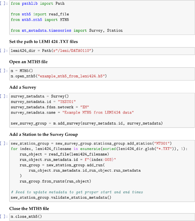
There are many ways a MTH5 file can be built with mth5. The most basic is to manually input metadata and data from a Python shell, but this should only be used for small changes. Most users will have data from a data logger, however each data logger may produce files in different formats with varying levels of metadata. For flexibility, a plug-in architecture is developed in mth5, where a plug-in reader can be built for specific data files, similar to ObsPy (Krischer et al., 2015). The only requirement is that the read_{data_logger} function in the plug-in must output a RunTS object with the appropriate metadata. For example, if the file type is made by an "example" data logger and the output files are .dat files, then a reader module would be developed with the name example that has a function read_example. This module would be added to the mth5.io module. The function and file types would then be added to the dictionary of available functions and associated file types that the main read function references. From the RunTS object, a station, run, and channel data sets can be added to an MTH5 file. Currently, there are plug-ins for Zonge International Z3D files, U.S. Geological Survey ASCII files, NIMS BIN files, LEMI424 long period ASCII files, and miniSEED files via ObsPy.

Figure 7: Example workflow for using a MTH5 file. A MTH5 file can be an archive format and a working format for processing. An MTH5 can be built from an archive or by reading from a data logger and adding metadata not included in the raw files. How data are transferred is archive dependent. For example, the IRIS DMC will send and receive miniSEED data files and StationXML metadata files. Note: tools exist in mth5 and mt_metadata to convert an MTH5 to and from miniSEED and StationXML.

Figure 8: Example code for how to build a MTH5 file from LEMI424 ASCII files. Note this is a simple example, in a real case much more metadata would need to be input and a new run should only be made if there is a time gap between files. Source code and example LEMI424 files can be found at https://github.com/kujaku11/mth5/tree/master/docs/examples/notebooks/example_01.ipynb.

4 Example Workflow

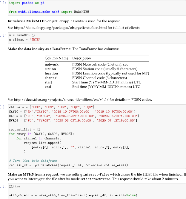
A MTH5 file is intended to be used both as a format for archiving and as a working format. Figure 7 schematically demonstrates an example workflow intended for data collected with IRIS PASSCAL MT instruments. Two ways to build a MTH5 file exist. First, data from a data logger are directly read into a MTH5 file with accompanying metadata not in the raw file, as described in Section 3.1.1 and Figure 8. Second, data are downloaded from the data logger, archived at the IRIS data managment center (DMC), and then retrieved to build a MTH5 file. This section is focused on the second method (Figure 9).

The IRIS DMC provides data in miniSEED (http://www.fdsn.org/pdf/SEEDManual_V2.4.pdf) and the metadata as a StationXML file (http://www.fdsn.org/xml/station/). This example uses tools developed in ObsPy for retrieving data and metadata from IRIS DMC. The user should know in advance what data they would like to request. IRIS provides many tools to query the DMC for available data (https://seiscode.iris.washington.edu/). The data will be represented as an ObsPy Stream object, which is a collection of synchronous channels. Tools are built in mth5.timeseries.RunTS to read in a Stream object. Then the process is similar to Section 3.1.1.

Figure 9: Example code for how to build a MTH5 file from the IRIS DMC. First, a data/metadata request is made, this can either be a CSV file or a Pandas DataFrame demonstrated here. If you do not know which data you would like you can use one of many tools provided by IRIS (https://seiscode.iris.washington.edu/). The request is done through ObsPy tools where a StationXML (metadata) and miniSEED (data) files are returned. These are converted into an Experiment (metadata) and RunTS objects (data) to be input into an MTH5 file through the function MakeMTH5.make_mth5_from_fdsnclient. Source code can be found at https://github.com/kujaku11/mth5/blob/master/docs/examples/notebooks/make_mth5_example_iris.ipynb.

5 Suggested Advances to support standardization of MT data and metadata

The current input/output plug-in architecture in mth5 only supports a couple data formats. As the user base grows, more data formats could be added by the community to allow for broader use. mt_metadata could be extended to include transfer functions to standardize reading and writing of various transfer function formats. Compliance checkers for metadata need to be developed, specifically XSD and JSON schema documents to allow for validation using XML and JSON tools. An open-source time series processing code is in development, funded through IRIS PASSCAL that uses MTH5 as the working format and mt_metadata to output transfer functions. Existing time series processing codes could be adjusted to work with MTH5 for better cohesion between various processing methods. A working group managed by the International Association of Geomagnetism and Aeronomy Division VI could be developed to support community driven changes to MT metadata and data standards, which could further support the adherence of MT data to FAIR principles.

6 Conclusions

The MT community has not had a standard format for time series data. Through community development a metadata standard and data format have been developed. The open-source Python packages mt_metadata and mth5 described in this study provide tools to help standardize MT time series data and make MT time series data more FAIR. Moving forward, MTH5 files will be the working format for data collected with IRIS PASSCAL MT instruments, the standard archive format for data collected by the U.S. Geological Survey, and the standard working format for a time series processing code currently in development by IRIS PASSCAL. Our release of the MT metadata standard, MTH5 time series data format and the associated open-source packages mt_metadata and mth5 can promote community development of these open-source tools, help standardize MT data in a FAIR way, and provide researchers less familiar with MT time series data with a good entry point to first-hand MT data analysis.

7 Acknowledgments

The authors would like to acknowledge the Working Group for Magnetotelluric Data Handling and Software members (Bruce Beaudoin, Lloyd Carothers, Jerry Carter, Gary Egbert, David Goldak, Maeva Pourpoint, Adam Schultz, Maxim Smirnov, Chad Trabant) for defining time series metadata. The authors would like to acknowledge Ben Murphy for help with fitting pole-zero filters to look-up tables. This project was partially funded by IRIS and the U.S. Geological Survey Community for Data Integration. The facilities of the IRIS Consortium are supported by the National Science Foundation’s Seismological Facilities for the Advancement of Geoscience Award under Cooperative Support Agreement EAR-1851048. Any use of trade, firm, or product names is for descriptive purposes only and does not imply endorsement by the U.S. Government.

Code availability section

mt_metadata

Contact: jpeacock@usgs.gov, 650-439-2833

Hardware requirements: …

Program language: Python 3.6+

Software required: Python

Program size: 2 Mb

The source codes are available for downloading at the link: https://doi.org/10.5281/zenodo.5605026

mth5

Contact: jpeacock@usgs.gov, 650-439-2833

Hardware requirements: …

Program language: Python 3.6+

Software required: Python

Program size: 2 Mb

The source codes are available for downloading at the link: https://doi.org/10.5281/zenodo.5637466

References

- Bedrosian et al. (2018) Bedrosian, P.A., Peacock, J.R., Bowles-Martinez, E., Schultz, A., Hill, G.J., 2018. Crustal inheritance and a top-down control on arc magmatism at Mount St Helens. Nature Geoscience 11, 865–870. doi:10.1038/s41561-018-0217-2.
- Chave and Jones (2012) Chave, A.D., Jones, A.G., 2012. The Magnetotelluric Method. Cambridge University Press. doi:10.1017/cbo9781139020138.
- Chave and Thomson (2004) Chave, A.D., Thomson, D.J., 2004. Bounded influence magnetotelluric response function estimation. Geophysical Journal International 157, 988–1006. doi:10.1111/j.1365-246X.2004.02203.x.
- Cordell et al. (2019) Cordell, D., Unsworth, M.J., Diaz, D., Reyes-Wagner, V., Currie, C.A., Hicks, S.P., 2019. Fluid and melt pathways in the Central Chilean subduction zone near the 2010 Maule Earthquake (35–36 S) as inferred from magnetotelluric data. Geochemistry, Geophysics, Geosystems 20, 1818–1835. doi:10.1029/2018gc008167.
- Egbert (2002) Egbert, G.D., 2002. Processing and interpretation of electromagnetic induction array data. Surveys in Geophysics 23, 207–249. doi:10.1023/A:1015012821040.
- Habermann et al. (2021) Habermann, T., Trabant, C., Ronan, T., Bahavar, M., Crosby, C., Dittman, T., Carter, J., Mencin, D., Suleiman, Y., Carothers, L., et al., 2021. Common data and metadata models for geophysical data in the cloud. Earth and Space Science Open Archive , 11doi:10.1002/essoar.10509909.1.
- Harris et al. (2020) Harris, C.R., Millman, K.J., van der Walt, S.J., Gommers, R., Virtanen, P., Cournapeau, D., Wieser, E., Taylor, J., Berg, S., Smith, N.J., Kern, R., Picus, M., Hoyer, S., van Kerkwijk, M.H., Brett, M., Haldane, A., del Río, J.F., Wiebe, M., Peterson, P., Gérard-Marchant, P., Sheppard, K., Reddy, T., Weckesser, W., Abbasi, H., Gohlke, C., Oliphant, T.E., 2020. Array programming with NumPy. Nature 585, 357–362. doi:10.1038/s41586-020-2649-2.
- Heinson et al. (2018) Heinson, G., Didana, Y., Soeffky, P., Thiel, S., Wise, T., 2018. The crustal geophysical signature of a world-class magmatic mineral system. Scientific Reports 8. doi:10.1038/s41598-018-29016-2.
- Hoyer et al. (2021) Hoyer, S., Hamman, J., Roos, M., Keewis, Cherian, D., Fitzgerald, C., Fujii, K., Maussion, F., Hauser, M., Crusaderky, Clark, S., Kleeman, A., Kluyver, T., Munroe, J., Amici, A., Nicholas, T., Barghini, A., Banihirwe, A., Gimperiale, Zac Hatfield-Dodds, Abernathey, R., Illviljan, Bell, R., Johnomotani, Roszko, M., Wolfram, P.J., Signell, J., Mühlbauer, K., Sinai, Y.B., Benoit Bovy, 2021. pydata/xarray: v0.18.2. doi:10.5281/ZENODO.4774304.
- Hoyer and Hamman (2017) Hoyer, S., Hamman, J.J., 2017. xarray: N-D labeled Arrays and Datasets in Python. Journal of Open Research Software 5. doi:10.5334/jors.148.
- Karaş et al. (2020) Karaş, M., Tank, S.B., Ogawa, Y., Oshiman, N., Matsushima, M., Honkura, Y., 2020. Probing the relationship between electrical conductivity and creep through upper crustal fluids along the western part of the North Anatolian Fault with three-dimensional magnetotellurics. Tectonophysics 791, 228561. doi:10.1016/j.tecto.2020.228561.
- Kelbert (2019) Kelbert, A., 2019. The Role of Global/Regional Earth Conductivity Models in Natural Geomagnetic Hazard Mitigation. Surveys in Geophysics 41, 115–166. doi:10.1007/s10712-019-09579-z.
- Kelbert (2020) Kelbert, A., 2020. EMTF XML: New data interchange format and conversion tools for electromagnetic transfer functions. Geophysics 85, F1–F17. doi:10.1190/geo2018-0679.1.
- Kelbert et al. (2011) Kelbert, A., Egbert, G.D., Schultz, A., 2011. Data Services Products: EMTF, The Magnetotelluric Transfer Functions. doi:10.17611/DP/EMTF.1.
- Kelbert et al. (2018) Kelbert, A., Erofeeva, S., Trabant, C., Karstens, R., Fossen, M.V., 2018. Taking Magnetotelluric Data out of the Drawer. EOS 99. doi:10.1029/2018eo112859.
- Klein and Taaheri (2016) Klein, L., Taaheri, A., 2016. HDF-EOS5 Data Model, File Format and Library. Tech Report ESDS-RFC-008v1.0. National Aeronautics and Space Administration.
- Krischer et al. (2015) Krischer, L., Megies, T., Barsch, R., Beyreuther, M., Lecocq, T., Caudron, C., Wassermann, J., 2015. ObsPy: a bridge for seismology into the scientific Python ecosystem. Computational Science & Discovery 8, 014003. doi:10.1088/1749-4699/8/1/014003.
- Krischer et al. (2016) Krischer, L., Smith, J., Lei, W., Lefebvre, M., Ruan, Y., de Andrade, E.S., Podhorszki, N., Bozdağ, E., Tromp, J., 2016. An Adaptable Seismic Data Format. Geophysical Journal International 207, 1003–1011. doi:10.1093/gji/ggw319.
- Lee (2012) Lee, J., 2012. GLAS_HDF detailed design. Tech Report. National Aeronautics and Space Administration.
- Loomis et al. (2019) Loomis, B.D., Luthcke, S.B., Sabaka, T.J., 2019. Regularization and error characterization of GRACE mascons. Journal of Geodesy 93, 1381–1398. doi:10.1007/s00190-019-01252-y.
- McKinney (2010) McKinney, W., 2010. Data structures for statistical computing in Python, in: Proceedings of the 9th Python in Science Conference, SciPy. doi:10.25080/majora-92bf1922-00a.
- Murphy et al. (2021) Murphy, B.S., Lucas, G.M., Love, J.J., Kelbert, A., Bedrosian, P.A., Rigler, E.J., 2021. Magnetotelluric sampling and geoelectric hazard estimation: are national-scale surveys sufficient? Space Weather 19. doi:10.1029/2020sw002693.
- Open Geospatial Consortium (2019) Open Geospatial Consortium, 2019. Geographic information — well-known text representation of coordinate reference systems. Technical Report. Open Geospatial Consortium, eds R. Lott. URL: http://docs.opengeospatial.org/is/18-010r7/18-010r7.html#8.
- Peacock et al. (2020) Peacock, J.R., Earney, T.E., Mangan, M.T., Schermerhorn, W.D., Glen, J.M., Walters, M., Hartline, C., 2020. Geophysical characterization of the Northwest Geysers geothermal field, California. Journal of Volcanology and Geothermal Research 399, 106882. doi:10.1016/j.jvolgeores.2020.106882.
- Peacock et al. (2021) Peacock, J.R., Frassetto, A., Kelbert, A., Egbert, G.D., Smirnov, M., Schultz, A., Kappler, K., Ronan, T., Trabant, C., 2021. Metadata standards for magnetotelluric time series data. U.S. Geological Survey data release. doi:https://doi.org/10.5066/P9AXGKEV.
- Reback et al. (2021) Reback, J., Jbrockmendel, McKinney, W., Van Den Bossche, J., Augspurger, T., Cloud, P., Hawkins, S., Roeschke, M., Gfyoung, Sinhrks, Klein, A., Hoefler, P., Terji Petersen, Tratner, J., She, C., Ayd, W., Naveh, S., JHM Darbyshire, Garcia, M., Shadrach, R., Schendel, J., Hayden, A., Saxton, D., Gorelli, M.E., Fangchen Li, Zeitlin, M., Jancauskas, V., McMaster, A., Battiston, P., Skipper Seabold, 2021. pandas-dev/pandas: Pandas 1.3.0. doi:10.5281/ZENODO.3509134.
- The HDF Group (2019) The HDF Group, 2019. HDF5 Users’s Guide: HDF5 Release 1.10. Technical Report. The HDF Group. URL: https://portal.hdfgroup.org/display/HDF5/HDF5UserGuides?preview=/53610087/53610088/Users_Guide.pdf.
- Wilkinson et al. (2016) Wilkinson, M.D., Dumontier, M., I. J. J. Aalbersberg, e., 2016. The FAIR Guiding Principles for scientific data management and stewardship. Scientific Data 3. doi:10.1038/sdata.2016.18.