Improved proof-by-contraction method and relative homologous entropy inequalities

Abstract

The celebrated holographic entanglement entropy triggered investigations on the connections between quantum information theory and quantum gravity. An important achievement is that we have gained more insights into the quantum states. It allows us to diagnose whether a given quantum state is a holographic state, a state whose bulk dual admits semiclassical geometrical description. The effective tool of this kind of diagnosis is holographic entropy cone (HEC), an entropy space bounded by holographic entropy inequalities allowed by the theory. To fix the HEC and to prove a given holographic entropy inequality, a proof-by-contraction technique has been developed. This method heavily depends on a contraction map $f$, which is very difficult to construct especially for more-region ($n\geq 4$) cases. In this work, we develop a general and effective rule to rule out most of the cases such that $f$ can be obtained in a relatively simple way. In addition, we extend the whole framework to relative homologous entropy, a generalization of holographic entanglement entropy that is suitable for characterizing the entanglement of mixed states.

1 Introduction

Recent progress in gravity/gauge duality has shed new light on our understanding of quantum gravity. For instance, a significant insight into the connections between quantum information theory and Anti-de Sitter/Conformal field theory (AdS/CFT) correspondence AdS/CFT1 ; AdS/CFT2 ; AdS/CFT3 was gained after the discovery of the holographic entanglement entropy (HEE), which states that area of a codimension-one homologous surface (the Ryu-Takayanagi (RT) surface) on a time slice is identified with the entanglement entropy in CFTs HEE1 ; HEE2

$$S(A)=\frac{\text{area}[m(A)]}{4G_{N}},$$ (1)

where $m(A)$ is a spacelike minimal hypersurface in the bulk spacetime, anchored to the asymptotic boundary such that $\partial m(A)=\partial A$. This remarkable formula provides direct evidence of the potential connections between quantum information theory and quantum gravity through holography. As a consequence, over the past few years a lot of efforts have been made to understand how this formula works in the holography community.

One significant achievement of these efforts is that it allows us to gain further insights into the quantum states. In particular, it provides an exact diagnosis on judging whether a given quantum field theory state has a holographic duals Heemskerk:2009pn . We usually call those states whose bulk duals admit semiclassical geometric descriptions the holographic states. These are a special sub-class of quantum states which satisfy certain constraints. A significant fact is that the RT formula (1) proved to be able to identify some of these constraints in the form of inequalities that the entropies of boundary subregions need to satisfy. In Bao:2015bfa , the authors found that, by arranging subsystem entropies of general mixed states into entropy vectors, entropy inequalities can be regarded as a space bounded by the allowed entropy vectors. It turns out that this is a convex space which has a configuration of a polyhedral cone and therefore is called the holographic entropy cone (HEC). HEC inequalities play a central role in understanding properties of holographic states. Therefore, what is the general structure of HEC and how to prove HEC inequalities become a key to the whole story. Over the last few years many progresses have been made in this direction, see for example the incomplete list HEC1 ; HEC2 ; HEC3 ; HEC4 ; HEC5 ; HEC6 . Among them, a proof technique for holographic entropy inequalities called proof-by-contraction was developed in Bao:2015bfa . It was latter generalized to more general cases in Rota:2017ubr ; Avis:2021xnz . Very recently, a geometric formulation of this method has been proposed in Bao:2015bfa ; Akers:2021lms . Given a general holographic entropy inequality

$$\sum_{l=1}^{L}\alpha_{l}S_{I_{l}}\geq\sum_{r=1}^{R}\beta_{r}S_{J_{r}}$$ (2)

where $S_{I}$ is RT entropy, $\alpha_{l},\beta_{r}$ are positive numbers, $L$ and $R$ are positive integers, representing the numbers of entropy terms appearing on each sides. The basic idea of the proof-by-contraction is to construct a reasonable rule such that one can compare terms in left-hand side (LHS) of (2) to the ones of right-hand side (RHS) in full generality. It was found in Bao:2015bfa that this can be achieved by finding a contraction map $f$: $\{0,1\}^{L}\rightarrow\{0,1\}^{R}$, where $\{0,1\}^{L}$ ( $\{0,1\}^{R}$) denotes a length-L (length-R) bitstrings formed by $0$ or $1$. One can introduce a weighted Hamming distance $d_{\omega}$ which is defined as

$$d_{\omega}(y,y^{\prime})\coloneqq\sum_{i=1}^{m}\omega_{i}\absolutevalue*{y_{i}-y^{\prime}_{i}},$$ (3)

where $\omega$ is a weight vector, and $y,y^{\prime}\in\{0,1\}^{m}$ are a pair of bitstrings. We can therefore prove that inequality (2) holds if there exists a contraction map $f$ for the weighted Hamming distances $d_{\alpha}$ and $d_{\beta}$ satisfying $d_{\alpha}(x,x^{\prime})\geq d_{\beta}(f(x),f(x^{\prime}))$ for every $x,x^{\prime}\in\{0,1\}^{L}$ Akers:2021lms .

One caveat, however, is that the difficulty of finding $f$ increases exponentially with the number of the terms in (2). If we use an exhaustive method to find $f(x)$ for all $x$, the number of all possible situations is of order $(2^{R})^{2^{L}}$ that is tremendous. We need to develop a general and effective rule to rule out most of the cases such that $f$ can be obtained in a relatively simple way. In this work, we develop a set of general rules to get $f$ effectively. Several examples are given to show the validity of our proposal.

In addition, our method is valid not only for RT entropy, but also for relative homologous entropy (RHE) Headrick:2017ucz , a well-defined generalization of holographic entanglement entropy that is suitable for characterizing the entanglement of mixed states. As an important example which has been studied widely in the past few years, the entanglement of purification (EoP) is a sub-class of RHE. See EoP ; Takayanagi:2017knl ; Nguyen:2017yqw ; EW1 ; EW2 ; EW3 ; HEoP1 ; HEoP2 ; HEoP3 ; HEoP4 ; HEoP5 ; HEoP6 ; HEoP7 ; HEoP8 ; HEoP9 ; HEoP10 ; HEoP11 ; HEoP12 ; HEoP13 ; HEoP14 ; HEoP15 ; HEoP16 ; HEoP17 ; HEoP18 ; HEoP19 ; HEoP20 ; HEoP21 ; HEoP22 ; HEoP23 ; HEoP24 ; HEoP25 ; HEoP26 for more recent progress on EoP and its holographic duality. Our analysis is based on the max flow-min cut (MFMC) theorem, which states that the maximum flux out of a boundary region $A$, optimized overall divergence free norm-bounded vector fields in the bulk, is proportional to the area of the minimal homologous surface $m(A)$ FH ; BT2 ; BT3 ; BT4 ; BT5 ; Agon:2021tia .

This paper is organized as follows: In section 2, we give a brief review on MFMC theorem and relative homology proposed in FH ; Headrick:2017ucz . In section 3, we first give an introduction to the proof-by-contraction method, then we generalize this method to relative homology and an improved version is developed. In section 4, we show how to devise a set of general rules to find the contraction map $f$. In section 5, several examples are given to show our method is valid. A concluding remark is given in the last section.

2 Brief review on MFMC theorem and relative homology

In this section we would like to give a brief review on the Riemannian MFMC theorem and relative homology in FH ; Headrick:2017ucz . First, let us begin with a compact oriented manifold $M$ with a conformal boundary $\partial M$. And define a “flow” on $M$, which is a vector field obeying

$$\nabla_{\mu}v^{\mu}=0,\qquad\absolutevalue{v}\leq 1.$$ (4)

We set $4G_{N}=1$ for convenience. Considering a subregion $A$ on boundary $\partial M$, the MFMC theorem says that there exists a max flow $v^{\mu}$ satisfying FH

$$\sup_{v^{\mu}}\int_{A}\sqrt{h}n_{\mu}v^{\mu}=\inf_{m\sim A}\text{Area}(m)\equiv S(A),$$ (5)

where $h$ is the determinant of the induced metric on $A$, $n_{\mu}$ is the normal vector. And $m$ is a bulk surface homologous to $A$ with condition $\partial A=\partial m$ (denote $m$ is homologous to $A$ as $m\sim A$). Where we have admitted the RT formula HEE1 in the second equal sign.

More generally, one can loosen the boundary condition on the bulk surface $m$ by introducing the concept of relative homology Headrick:2017ucz . Assume there is a surface $R$, which could be either on a boundary or in bulk. And $m^{\prime}$ is the surface homologous to $A$, which is allowed to include part of $R$. Then we can define a surface $m$ homologous to $A$ relative to $R$ as

$$m\coloneqq-(m^{\prime}\setminus R)$$ (6)

excluding the part on $R$, which is denoted as $m\sim A\text{ rel }R$. Where the minus sign means that $m$ takes different orientation relative to $m^{\prime}$. See the Fig. 1(a).

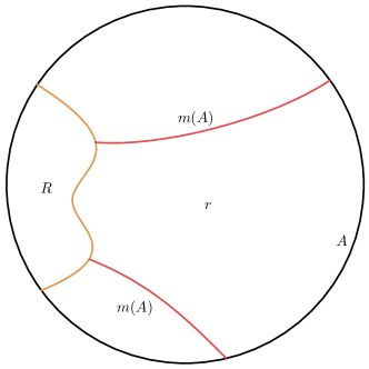
(a) Relative homology for one system

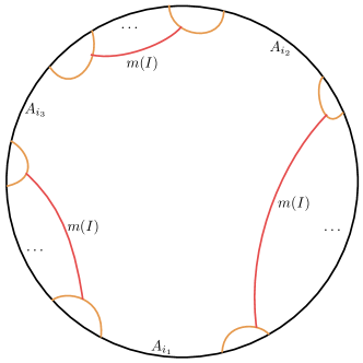
(b) Relative homology for multiple systems

Figure 1: (a) Relative homology for single boundary region $A$: the orange line represents relative surface $R$, the red lines $m(A)$ are homologous to $A$ relative to $R$, and $r$ is the bulk region enclosed by $A,m(A)$ and $R$. (b) Relative homology for multiple boundary regions: orange lines still represent $R$, red lines $m(I)$ are homologous to $A_{I}$ relative to $R$, where $I=\{i_{1},i_{2},i_{3}\}$. We eliminate the bulk part that enclosed by $R$ and $\partial M$, then we get $M^{\prime}$, i.e., the bulk region enclosed by $A$ and $R$.

Let us now turn to the MFMC theorem associated with relative homology. This is a direct generalization of the original MFMC theorem, that is Headrick:2017ucz

$$\sup_{\begin{subarray}{c}v^{\mu}:\\ n_{\mu}v^{\mu}|_{R}=0\end{subarray}}\int_{A}\sqrt{h}n_{\mu}v^{\mu}=\inf_{\begin{subarray}{c}m\sim A\\ \text{rel }R\end{subarray}}\ \text{Area}(m),$$ (7)

where $h$ is the determinant of the induced metric on $A$, $n_{\mu}$ is the normal vector on $A\cup R$, and we impose a Neumann condition (no-flux condition) on $R$ for the flow. Note that the MFMC theorem shows us the equivalency between “max-flow” and “min-cut”.

Following RT formula, define a so-called relative homologous entropy (RHE) Headrick:2017ucz as

$$\tilde{S}_{A}\coloneqq\inf_{\begin{subarray}{c}m\sim A\\ \text{rel }R\end{subarray}}\text{Area}(m)=\sup_{\begin{subarray}{c}v^{\mu}:\\ n_{\mu}v^{\mu}|_{R}=0\end{subarray}}\int_{A}\sqrt{h}n_{\mu}v^{\mu}.$$ (8)

The above definition can be directly generalized to multiple boundary regions. Consider $n$ non-overlapping boundary regions $A_{i}$ $(i\in[n]\coloneqq\{1,\dots,n\})$ on $\partial M$. We can choose a particular surface $R$ on $M$, whose boundary satisfying $\partial R=\bigcup_{i\in[n]}\partial A_{i}$. So that $R$ and $A_{i}$ $(i\in[n])$ enclose an open bulk region $M^{\prime}$, as shown in Fig. 1(b).

For boundary region $A_{I}\equiv\bigcup_{i\in I}A_{i}$, where $I$ is a nonempty subset of $[n]$, we have

$$\tilde{S}_{I}\coloneqq\inf_{\begin{subarray}{c}m(I)\sim A_{I}\\ \text{rel }R\end{subarray}}\text{Area}(m(I))=\text{Area}[\tilde{m}(I)],$$ (9)

where bulk surface $m(I)$ is homologous to $A_{I}\equiv\bigcup_{i\in I}A_{i}$ relative to $R$, and $\tilde{m}(I)$ is defined as the minimal relative homologous (RH) surface of $A_{I}$.

For the following discussion, we should mention that the status of $M^{\prime}$ in the RHE inequality is the same as the status of $M$ in the HEE inequality. The Neumann boundary condition $n_{\mu}v^{\mu}=0$ defined on $R$ implies that the flow (or bit thread) can not be allowed to get through $R$. Thus a max flow emerging from $A_{I}$ must get through the minimum RH surface $\tilde{m}(I)$ and eventually arrive at $A_{[n]\backslash I}$, similarly for $A_{[n]\backslash I}$. So $\tilde{m}(I)$ and $\tilde{m}([n]\backslash I)$ are identical, it implies that RHE and HEE are extremely similar from the inequality perspective.

And note that when $R$ is chosen to be empty set , RHE will become HEE FH ; Headrick:2017ucz . Or we can choose $R$ to be min RT surface of some $A_{I}$, then RHE can reproduce holographic entanglement wedge cross section proposal DCS ; HHea . While in the following, we will study the general inequality properties of RHE (9) from the “cut” side on a geometric perspective.

3 Improved proof-by-contraction method

3.1 Brief review on proof-by-contraction method

The RT formula reveals a deep connection between the bulk geometry and boundary entanglement structures, which promotes us to study the inequalities of entanglement entropy from a geometrical perspective.

A direct way is the following: if we can use some minimal RH surface of some union region $A_{I_{l}}(l=1,2,\cdots,L)$ to get new RH surface (usually not minimal) of other union region $A_{J_{r}}(r=1,2,\cdots,R)$, then we can have inequalities about $S_{I_{l}}$ and $S_{J_{r}}$. See more specific descriptions in the following.

Minimum homologous surface of union region appearing on the left of inequality would be cut into fragments by themselves since they may cross each other. Proof-by-contraction method is a way to paste the surface fragments cut by themselves into homologous surface (usually not minimum) of union region appearing on the right of inequality. Contraction map $f$ that we will introduce soon is the key to how surface fragments are pasted. The whole process can be simply written as cut-$f$-paste or just cut-paste.

Generally an inequality for RHE can be written as Akers:2021lms

$$\sum_{l=1}^{L}\alpha_{l}\tilde{S}_{I_{l}}\geq\sum_{r=1}^{R}\beta_{r}\tilde{S}_{J_{r}},$$ (10)

where $\alpha_{l},\beta_{r}$ are positive numbers (usually they are rational number, so we can multiply them by a large enough integer to get integer), $L$ and $R$ are positive integers, representing the numbers of RHE terms appearing on each side. $I_{l},J_{r}\subseteq[n]$ and $\forall\ l\neq l^{\prime},r\neq r^{\prime}$, we have $I_{l}\neq I_{l^{\prime}},J_{r}\neq J_{r^{\prime}},I_{l}\neq J_{r}$. The only difference between (2) and (10) is that we have replaced the RT entropy $S$ in (2) by the RHE $\tilde{S}$.

To construct the inequality, we need to cut the bulk $M^{\prime}$ by using the minimum RH surface $\tilde{m}(I_{l})$ of union regions $A_{I_{l}}$. So these boundaries of bulk pieces are the fragments of min RH surface. The surface fragments can also be used to reconstruct the $\tilde{S}_{I_{l}}$ by pasting them back.

Then we try to paste these surface fragments to get RH surface of union regions $J_{r}$. If we have inequality as follows,

$$\sum_{l=1}^{L}\alpha_{l}\text{Area}[\tilde{m}(I_{l})]\geq\sum_{r=1}^{R}\beta_{r}\text{Area}[m^{\prime}(J_{r})],$$ (11)

where $m^{\prime}(J_{r})$ is the RH surface (usually not minimal) and we will prove the general inequality immediately. In what follows we will show how to find RH surfaces of $J_{r}$ for all $r=1,\cdots,R$ that satisfy inequality (11).

3.2 Cut by left min RH surface

To proceed, let us define an open bulk subregion $\sigma_{I}$ on $M^{\prime}$, called RH bulk region, which satisfies $\partial\sigma_{I}=\tilde{m}(I)\cup A_{I}$. We cut $M^{\prime}$ by $\tilde{m}(I_{l})$ for all $l=1,\dots,L$. These $\tilde{m}(I_{l})$ will cut $M^{\prime}$ into $2^{L}$ pieces (possibly including some empty pieces). Then we encode these bulk pieces with length-$L$ bitstrings $x\in\{0,1\}^{L}$

$$\sigma(x)\coloneqq\bigcap_{l=1}^{L}\sigma_{I_{l}}^{x_{l}},\qquad\sigma_{I}^{b}=\left\{\begin{matrix}\sigma_{I}&\text{if }b=1,\\ \sigma_{I}^{\complement}&\text{if }b=0,\end{matrix}\right.$$ (12)

where $x_{l}$ is the $l^{th}$ component of $x$ and $\sigma_{I}^{\complement}$ is the complement of $\sigma_{I}$ defined as $M^{\prime}\setminus\sigma_{I}$. $\sigma(x)$ may be empty for some $x$. It is easy to get $\forall x\neq x^{\prime},\sigma(x)\cap\sigma(x^{\prime})=\emptyset$ by definition (12). The surface fragment can be written as

$$m(x,x^{\prime})\coloneqq\overline{\sigma(x)}\bigcap_{\text{codim-1}}\overline{\sigma(x^{\prime})},$$ (13)

where $\overline{\sigma(x)}$ represents the closure of the corresponding region $\sigma(x)$, and codim-1 means that we will calculate the area by using the integral measure of $m(x,x^{\prime})$ in codimension-1 manifold. If dimension of $m(x,x^{\prime})$ is less than codimension-1, then the area of $m(x,x^{\prime})$ is zero. We also need to require $x\neq x^{\prime}$, otherwise $m(x,x)$ is just $\overline{\sigma(x)}$ whose dimension is codimension-0 and the area of $m(x,x)$ will go to infinity. As shown in Fig. 2, the shaded bulk region corresponding to $\sigma_{I_{1}}$. And the $\sigma(x)$ are denoted by the bitstrings $x$ in the figure, such as $"00"$ represents the open bulk region $\sigma(00)$ and so on.

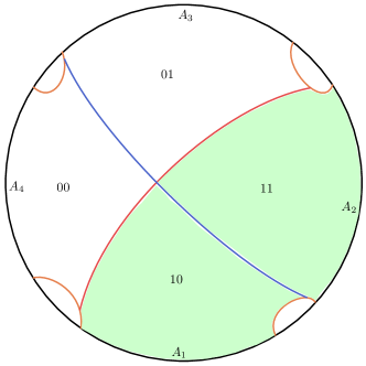
Figure 2: Consider the SSA, i.e. $S_{A_{1}A_{2}}+S_{A_{2}A_{3}}\geq S_{A_{2}}+S_{A_{1}A_{2}A_{3}}$. The orange, red and blue lines represent the relative regions $R$, $\tilde{m}(I_{1})$ and $\tilde{m}(I_{2})$ respectively, where $I_{1}=\{1,2\},I_{2}=\{2,3\}$. Where the shaded region denotes $\sigma_{I_{1}}$.

By using these bulk pieces and surface fragments, we can reconstruct $\sigma_{I_{l}}$ and min RH surface

$$\sigma_{I_{l}}=\bigcup_{x:x_{l}=1}\sigma(x).$$ (14)

This can be achieved directly from definition (12). In addition, we can also get $\tilde{m}(I_{l})$ as

$$\tilde{m}(I_{l}) \coloneqq\overline{\sigma_{I_{l}}}\bigcap_{\text{codim-1}}\overline{\sigma_{I_{l}}^{\complement}}$$

$$=\left(\overline{\bigcup_{x:x_{l}=1}\sigma(x)}\right)\bigcap_{\text{codim-1}}\left(\overline{\bigcup_{x^{\prime}:x^{\prime}_{l}=0}\sigma(x^{\prime})}\right)$$

$$=\left(\bigcup_{x:x_{l}=1}\overline{\sigma(x)}\right)\bigcap_{\text{codim-1}}\left(\bigcup_{x^{\prime}:x^{\prime}_{l}=0}\overline{\sigma(x^{\prime})}\right)$$

$$=\bigcup_{x,x^{\prime}:x_{l}\neq x^{\prime}_{l}}m(x,x^{\prime}).$$

The second line stems from Eq. (14). In the fourth line we use the distribution law and the definition  (13). While in the third line we have used that

$$\left\{\begin{array}[]{l}\overline{\bigcup\sigma(x)}=\partial\left(\bigcup\sigma(x)\right)\cup\left(\bigcup\sigma(x)\right)\subseteq\bigcup(\overline{\sigma(x)})\\ \bigcup(\overline{\sigma(x)})=\bigcup(\partial\sigma(x)\cup\sigma(x))=\left(\bigcup\partial\sigma(x)\right)\cup\left(\bigcup\sigma(x)\right)\subseteq\overline{\bigcup\sigma(x)}\end{array}\right.$$

$$\Rightarrow \left\{\begin{array}[]{l}\overline{\bigcup\sigma(x)}\subseteq\bigcup(\overline{\sigma(x)})\\ \bigcup(\overline{\sigma(x)})\subseteq\overline{\bigcup\sigma(x)}\end{array}\right.\Rightarrow\overline{\bigcup\sigma(x)}=\bigcup\overline{\sigma(x)}.$$

In a word, we have

$$\tilde{m}(I_{l})=\bigcup_{x,x^{\prime}:x_{l}\neq x^{\prime}_{l}}m(x,x^{\prime}).$$ (15)

The RHE $\tilde{S}_{I_{l}}$ then can be obtained by definition

$$\tilde{S}_{I_{l}} =\text{Area}[\tilde{m}(I_{l})]=\sum_{\begin{subarray}{c}x,x^{\prime}:\\ x_{l}=1,x^{\prime}_{l}=0\end{subarray}}\text{Area}[m(x,x^{\prime})]$$

$$=\frac{1}{2}\sum_{x,x^{\prime}}|x_{l}-x^{\prime}_{l}|\text{Area}[m(x,x^{\prime})].$$ (16)

Since $\forall(x^{1},{x^{1}}^{\prime})\neq(x^{2},{x^{2}}^{\prime})$ and $\text{Area}[m(x^{1},{x^{1}}^{\prime})\cap m(x^{2},{x^{2}}^{\prime})]=0$, we can directly add the area of $m(x,x^{\prime})$ for different $(x,x^{\prime})$ pair. Due to the symmetry between $x$ and $x^{\prime}$, there is a prefactor $1/2$ in the last term.

3.3 Paste into right RH surface

We already know how to get surface fragments and reconstruct min RH surface using these fragments. The purpose is constructing the RH surface of $J_{r}$ by these fragments.

The first step is to know the difference between RH surface and ordinary surface region. It turns out that, differing from ordinary surface region, $J_{r}$ and its RH surface form a bulk region $\overline{\sigma_{J_{r}}}$ which only contains union region $A_{J_{r}}$. Mathematically, this corresponds to

$$\overline{\sigma_{J_{r}}}\supseteq A_{J_{r}}=\bigcup_{i\in J_{r}}A_{i},$$

$$\overline{\sigma_{J_{r}}}\nsupseteq A_{j}(j\notin J_{r})\text{\quad or\quad}\overline{\sigma_{J_{r}}^{\complement}}\supseteq A_{[n]\setminus J_{r}}=\bigcup_{i\notin J_{r}}A_{i}.$$ (17)

Above restriction implies $\sigma_{J_{r}}$ is bounded. We take an example to specify the bound as follow. Let us consider a monogamy-like inequality of RHE (the formal proof will be given in 5.2): $\tilde{S}_{A_{1}A_{2}}+\tilde{S}_{A_{1}A_{3}}+\tilde{S}_{A_{2}A_{3}}\geq\tilde{S}_{A_{1}}+\tilde{S}_{A_{2}}+\tilde{S}_{A_{3}}+\tilde{S}_{A_{1}A_{2}A_{3}}$, where $I_{1}=\{1,2\},I_{2}=\{1,3\},I_{3}=\{2,3\},J_{1}=\{1\}$. Then we get the bound of $\sigma_{J_{1}}$ by Eq. (17), as seen in Fig. 3.

The next step is to construct $\sigma_{J_{r}}$. Only by using bulk pieces $\sigma(x)$ can we construct $\sigma_{J_{r}}$ to get $m^{\prime}(J_{r})$. As suggested in Akers:2021lms , we can connect $\sigma_{J_{r}}$ and $\sigma(x)$ by setting a contraction map $f:\{0,1\}^{L}\rightarrow\{0,1\}^{R}$. Similar to Eq. (14), one can define $\sigma_{J_{r}}^{\prime}$

$$\sigma_{J_{r}}^{\prime}\coloneqq\bigcup_{x:f(x)_{r}=1}\sigma(x),$$ (18)

where $f(x)_{r}$ is the $r^{th}$ component of $f(x)\in\{0,1\}^{R}$. However, up to now $\sigma_{J_{r}}^{\prime}$ represents nothing since no constraint has been imposed on $f$ yet. Recalling that we would like to construct $\sigma_{J_{r}}$ from $\sigma(x)$. Thus, if we treat $\sigma_{J_{r}}^{\prime}$ as $\sigma_{J_{r}}$, this can be achieved by definition (21). In this case, $\sigma_{J_{r}}^{\prime}$ must satisfy constraint (17), which in turn will impose some constraints on $f$. In what follows, we would like to show how to put constraints on $f$.

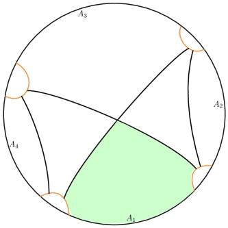
(a) lower bound

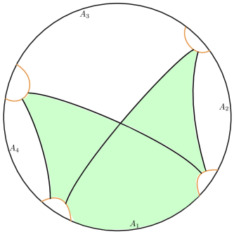
(b) upper bound

Figure 3: The lower bound of $\sigma_{J_{1}}$ is shown in (a) and the upper bound of $\sigma_{J_{1}}$ is shown (b). The lower bound means intersection of all $\sigma_{J_{r}}$ defined by eq. (21) and the upper bound means union of all the $\sigma_{J_{r}}$. All $\overline{\sigma_{J_{1}}}$ bounded by eq. (17) contain RH surface of $A_{1}$. If $\overline{\sigma_{J_{1}}}$ is not bounded by eq. (17), then $\partial\sigma_{J_{1}}\setminus A_{1}$ will not correspond to RH surface of $A_{1}$.

So the third step is to add some basic constraints on $f$. First we should find all $\sigma(x)$ that only contains $A_{i}$. Using $x^{(i)}$ to code the $\sigma(x^{(i)})$ that only contains $A_{i}$ and it can be written as

$$x^{(i)}_{l}=\chi_{I_{l}}\equiv\left\{\begin{matrix}1&i\in I_{l},\\ 0&i\notin I_{l},\end{matrix}\right.$$ (19)

where $\chi_{I_{l}}$ is a characteristic function defined by above equation.

Then we restrict $f$ so that $\sigma_{J_{r}}^{\prime}$ satisfies constraint (17), that is,

$$f(x^{(i)})_{r}=\chi_{J_{r}}\equiv\left\{\begin{matrix}1&i\in J_{r},\\ 0&i\notin J_{r},\end{matrix}\right.$$ (20)

where $\chi_{J_{r}}$ is also a characteristic function.

We will no longer distinguish $\sigma_{J_{r}}^{\prime}$ and $\sigma_{J_{r}}$ from now on, since we have already required $\sigma_{J_{r}}^{\prime}$ to satisfy (17) by restricting $f$. Thus we have

$$\sigma_{J_{r}}=\bigcup_{x:f(x)_{r}=1}\sigma(x).$$ (21)

Now we can follow what we did in getting $\tilde{m}(I_{l})$ to obtain $m^{\prime}(J_{r})$ immediately,

$$m^{\prime}(J_{r}) \coloneqq\overline{\sigma_{J_{r}}}\bigcap_{\text{codim-1}}\overline{\sigma_{J_{r}}^{\complement}}$$

$$=\left(\overline{\bigcup_{x:f(x)_{r}=1}\sigma(x)}\right)\bigcap_{\text{codim-1}}\left(\overline{\bigcup_{x^{\prime}:f(x^{\prime})_{r}=0}\sigma(x^{\prime})}\right)$$

$$=\left(\bigcup_{x:f(x)_{r}=1}\overline{\sigma(x)}\right)\bigcap_{\text{codim-1}}\left(\bigcup_{x^{\prime}:f(x^{\prime})_{r}=0}\overline{\sigma(x^{\prime})}\right)$$

$$=\bigcup_{\begin{subarray}{c}x,x^{\prime}:\\ f(x)_{r}\neq f(x^{\prime})_{r}\end{subarray}}m(x,x^{\prime}).$$

In the end, following eq (16), we get the RHE for $J_{r}$,

$$\tilde{S}_{J_{r}} =\text{Area}[\tilde{m}(J_{r})]\leq\text{Area}[m^{\prime}(J_{r})]$$

$$=\sum_{\begin{subarray}{c}x,x^{\prime}:\\ f(x)_{r}=1\\ f(x^{\prime})_{r}=0\end{subarray}}\text{Area}[m(x,x^{\prime})]=\frac{1}{2}\sum_{x,x^{\prime}}|f(x)_{r}-f(x^{\prime})_{r}|\text{Area}[m(x,x^{\prime})].$$ (22)

3.4 Inequality of weight distance

Now we are stepping to show how it means if the inequality (10) holds. From Eqs. (16) and (22), we can see that if

$$\sum_{l=1}^{L}\alpha_{l}\frac{1}{2}\sum_{x,x^{\prime}}|x_{l}-x^{\prime}_{l}|\text{Area}[m(x,x^{\prime})]\geq\sum_{r=1}^{R}\beta_{r}\frac{1}{2}\sum_{x,x^{\prime}}|f(x)_{r}-f(x^{\prime})_{r}|\text{Area}[m(x,x^{\prime})]$$ (23)

holds, then the inequality (10) holds identically. While (23) can be rewritten as

$$\sum_{x,x^{\prime}}\sum_{l=1}^{L}\alpha_{l}|x_{l}-x^{\prime}_{l}|\text{Area}[m(x,x^{\prime})]\geq\sum_{x,x^{\prime}}\sum_{r=1}^{R}\beta_{r}|f(x)_{r}-f(x^{\prime})_{r}|\text{Area}[m(x,x^{\prime})].$$ (24)

Therefore, if we define a weight distance $d_{\omega}(y,y^{\prime})$ by

$$d_{\omega}(y,y^{\prime})\coloneqq\sum_{i}\omega_{i}\absolutevalue*{y_{i}-y^{\prime}_{i}},$$ (25)

where $y_{i},y^{\prime}_{i}$ are the $i^{\text{th}}$ component of $y,y^{\prime}$, then we get

$$\forall(x,x^{\prime})\in\{(x,x^{\prime}):\text{Area}[m(x,x^{\prime})]\neq 0\text{ and }x,x^{\prime}\in\{0,1\}^{L}\},$$

$$d_{\alpha}(x,x^{\prime})\geq d_{\beta}(f(x),f(x^{\prime}))\Rightarrow\sum_{l=1}^{L}\alpha_{l}\tilde{S}_{I_{l}}\geq\sum_{r=1}^{R}\beta_{r}\tilde{S}_{J_{r}}.$$ (26)

So the problem has already been transformed from finding $m^{\prime}(J_{r})$ to finding $f$ satisfying basic constraints (17) and inequality of weight distance $d_{\alpha}(x,x^{\prime})\geq d_{\beta}(f(x),f(x^{\prime}))$ for all $(x,x^{\prime}):\text{Area}[m(x,x^{\prime})]\neq 0$, since $m^{\prime}(J_{r})$ is defined by $\sigma_{J_{r}}$ which is completely determined by $f$. If we find $f$ that satisfies the conditions, we prove the inequality (10). We should emphasize, however, that if we cannot find $f$ satisfying the conditions $d_{\alpha}(x,x^{\prime})\geq d_{\beta}(f(x),f(x^{\prime}))$, it does not mean the inequality of RHE is false. In other words, condition $d_{\alpha}(x,x^{\prime})\geq d_{\beta}(f(x),f(x^{\prime}))$ is a sufficient condition but is not a necessary one.

In the next section we will establish a general method to find $f$.

4 Method of finding contraction map

If an exhaustive method is used to find $f(x)$ for all $x$, the number of all situations of $f$ will be the order of $(2^{R})^{2^{L}}$, which is an astronomical number. Only rule out most cases can we find $f$ in a relatively simple way. If we take a look at (26) carefully, it implies there exist three conditions for $f$ and $(x,x^{\prime})$ needed to be obeyed, namely nonempty bulk pieces of $x$, $\text{Area}[m(x,x^{\prime})]\neq 0$ and $d_{\alpha}(x,x^{\prime})\geq d_{\beta}(f(x),f(x^{\prime}))$. Hence, it turns out one can find $f$ by the following steps:

• First, we should exclude the bitstrings $x$ corresponding to empty bulk pieces. We will show that all bitstrings $x$ of empty bulk piece form a sub-set of all $x$ whose $g(x)$ is not equal to $\{1\}^{L^{2}}$, where $g(x)$ is defined in the following in Eq. (27).

• Second, we should exclude the $(x,x^{\prime})$ which corresponds to zero-area contribution, i.e., those corresponding to $\text{Area}[m(x,x^{\prime})]=0$. We will show that only for pairs $(x,x^{\prime})$ with unit distance can $m(x,x^{\prime})$ contribute nonzero area. The distance of $(x,x^{\prime})$ denoted by $d(x,x^{\prime})$ is defined as $d_{\alpha}(x,x^{\prime})$, where $\alpha_{l}=1$, and $l=1,\dots,L$.

• Third, we then find $f(x)$ of $x$ corresponding to nonempty bulk piece. After requiring that $\forall x,x^{\prime}\in\mathbb{B}$, $f$ satisfies inequality of weight distance, one can finally find the map $f$. We will give the detailed steps to find these $f(x)$ in section 4.3.

4.1 Exclude empty bulk piece

As a first step, let us define a mapping $g$ so as to distinguish whether $x$ correspond to empty bulk piece or not. To proceed, we define $I^{0}\coloneqq[n]\setminus I,I^{1}\coloneqq I$. Then we define mapping $g$ as follow

Definition 1.

Let $g$ be a map from $\{0,1\}^{L}$ to $\{0,1\}^{L^{2}}$ and $g(x)_{l,l^{\prime}}$ is the $[(l-1)L+l^{\prime}]^{\text{th}}$ component of $g(x)$, and

$$g(x)_{l,l^{\prime}}=\left\{\begin{matrix}1,&I_{l}^{x_{l}}\cap I_{l^{\prime}}^{x_{l^{\prime}}}\neq\emptyset,\\ 0,&I_{l}^{x_{l}}\cap I_{l^{\prime}}^{x_{l^{\prime}}}=\emptyset.\end{matrix}\right.$$ (27)

Lemma 1.

Min RH surfaces of two non-overlapping systems $A,B$ do not cross and the intersection of their RH bulk regions denoted as $\sigma_{A}\cap\sigma_{B}$ is empty.

Proof.

Suppose two non-overlapping systems $A,B$ and their min RH surfaces $\tilde{m}(A),\tilde{m}(B)$. Their RH regions are $\sigma_{A},\sigma_{B}$ formed by $A,B$ and $\tilde{m}(A),\tilde{m}(B)$.

Now let us assume that $\tilde{m}(A),\tilde{m}(B)$ will cross, then we get $\sigma_{A}\cap\sigma_{B}\neq\emptyset$ as shown in Fig. 4. In this case, we find that $(\tilde{m}(A)\setminus\partial(\sigma_{A}\cap\sigma_{B}))\cup(\tilde{m}(B)\cap\partial(\sigma_{A}\cap\sigma_{B}))$ is still a RH surface of $A$. Without loss of generality, let us assume $\text{Area}[\partial(\sigma_{A}\cap\sigma_{B})\cap\tilde{m}(B)]<\text{Area}[\partial(\sigma_{A}\cap\sigma_{B})\cap\tilde{m}(A)]$, then $\text{Area}[(\tilde{m}(A)\setminus\partial(\sigma_{A}\cap\sigma_{B}))\cup(\tilde{m}(B)\cap\partial(\sigma_{A}\cap\sigma_{B}))]<\text{Area}[\tilde{m}(A)]$ which is contradiction with the fact that $\tilde{m}(A)$ is the min RH surface of $A$. The discussion is same for $B$. ∎

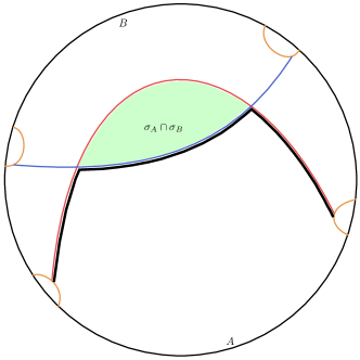
Figure 4: The red line is $\tilde{m}(A)$, the blue line is $\tilde{m}(B)$ and the green shadow is $\sigma_{A}\cap\sigma_{B}$. And the black outline is $(\tilde{m}(A)\setminus\partial(\sigma_{A}\cap\sigma_{B}))\cup(\tilde{m}(B)\cap\partial(\sigma_{A}\cap\sigma_{B})$.

Theorem 1.

$x$ corresponds to an empty bulk piece if $g(x)$ is not equal to $\{1\}^{L^{2}}$, where $\{1\}^{L^{2}}$ means $\forall\ l,l^{\prime},g(x)_{l,l^{\prime}}=1$.

Proof.

According to Lemma. 1, we can get that $\tilde{m}(I)$ and $\tilde{m}(I^{\prime})$ do not intersect when $I\cap I^{\prime}=\emptyset$. In addition, $\tilde{m}(I)$ and $\tilde{m}(I^{\prime})$ still do not intersect if we have $I\cap([n]\setminus I^{\prime})=\emptyset$ instead of $I\cap I^{\prime}=\emptyset$, since $\tilde{m}(I)=\tilde{m}([n]\setminus I)$ holds by choosing $R=\{R\in M:\partial R=\bigcup_{i\in[n]}\partial A_{i}\}$.

If $g(x)\neq\{1\}^{L^{2}}$, then $\exists\ l,l^{\prime},g(x)_{l,l^{\prime}}=0$. According to Definition. 27 and above statement, we will get $\sigma(x)\subseteq\sigma_{I_{l}}^{x_{l}}\cap\sigma_{I_{l^{\prime}}}^{x_{l^{\prime}}}=\emptyset$, which exactly means that $x$ corresponds to an empty bulk piece. ∎

We will denote the supset of all $x$ encoding nonempty bulk pieces by $\mathbb{B}$. In other words, for every $x$ encoding nonempty bulk pieces, $x\in\mathbb{B}$. That is, we define $\mathbb{B}$ as

$$\mathbb{B}\coloneqq\{x:g(x)=\{1\}^{L^{2}}\text{ and }x\in\{0,1\}^{L}\}.$$ (28)

In summary, we only need to find $f(x)$ for nontrivial $x\in\mathbb{B}$, since $f(x)$ for trivial $x\in\{x:g(x)\neq\{1\}^{L^{2}}\}$ will not affect inequality (10).

4.2 Exclude surface fragment of zero-area contribution

Now we would like to find all pair $(x,x^{\prime})$ whose corresponding $m(x,x^{\prime})$ with nonzero area contribution. Such $(x,x^{\prime})$ have a close relationship with $d(x,x^{\prime})$ as we will see.

Definition 2.

Let $\sigma_{I_{l}}(l=1,\dots,L)$ be an open set and we can generate a topology $\mathcal{T}$ that is a set of open subsets of $M^{\prime}$ satisfying:

• $\emptyset,M^{\prime},\sigma_{I_{1}},\dots,\sigma_{I_{L}}\in\mathcal{T}$,

• $\forall\alpha\in\Lambda$ where $\Lambda$ is some either finite or infinite set, $O_{\alpha}\subset M^{\prime}$, if $\{O_{\alpha}\}_{\alpha\in\Lambda}\subseteq\mathcal{T}$, then $\bigcup_{\alpha\in\Lambda}O_{\alpha}\in\mathcal{T}$,

• $m\in\mathbb{N}$, $\forall i\in[m],O_{i}\subset M^{\prime}$, if $\{O_{i}\}_{i\in[m]}\subseteq\mathcal{T}$, then $\bigcap_{i=1}^{m}O_{i}\in\mathcal{T}$.

Definition 3.

Let $(x,x^{\prime})$ be a pair where $x,x^{\prime}\in\mathbb{B}$. $(x,x^{\prime})$ is directly connected if and only if only one component of $x$ and $x^{\prime}$ is different. $(x,x^{\prime})$ is connected if there is a path, for all $x^{i}\in\mathbb{B},(i=1,\cdots,n)$ on the path, $(x^{i},x^{i+1})$ is always directly connected where $x^{1}=x$ and $x^{n}=x^{\prime}$.

For example, we can see Fig. 2 where $(00,01),(00,10),(01,11),(10,11)$ are all directly connected. And according to Definition. 3, $(00,11),(01,10)$ are connected since there are paths $00\rightarrow 01\rightarrow 11$ and $01\rightarrow 00\rightarrow 10$ connecting $00,11$ and $01,10$ where $(00,01),(01,11)$ and $(01,00),(00,10)$ are directly connected. We should mention that two geometrically joint regions $\sigma(x)$ and $\sigma(x^{\prime})$ do not always mean that the corresponding pairs $(x,x^{\prime})$ are directly connected and vice versa. One explicit example is depicted in Fig. 5.

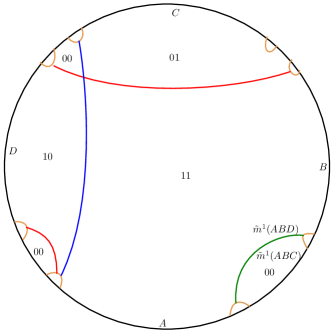
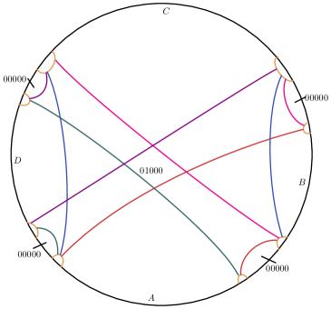
Figure 5: (a) Example that $\sigma(x)$ and $\sigma(x^{\prime})$ are geometrical neighbors while the corresponding pairs $(x,x^{\prime})$ are NOT directly connected. Let $I_{1}=ABC,I_{2}=ABD$, then $\sigma(00)$ and $\sigma(11)$ are geometrical neighbors, while the corresponding pairs ($x=00,x^{\prime}=11$) are not directly connected. Note that in this case the surface fragments $\tilde{m}^{1}(ABC)$ and $\tilde{m}^{1}(ABD)$ are overlapped and are marked by green line. (b) Example that $(x,x^{\prime})$ are directly connected while the corresponding relative regions $\sigma(x)$ and $\sigma(x^{\prime})$ are NOT geometrical neighbors. Let $I_{1}=AB,I_{2}=AC,I_{3}=AD,I_{4}=BC,I_{5}=CD$, then $(00000,01000)$ is directly connected, while $\sigma(01000)$ and $\sigma(00000)$ are not geometrical neighbors.

Definition 4.

Let $m_{l}(x)$ encoded by $x\in\{0,1\}^{L}$ be a fragment of $\tilde{m}(I_{l})$ cut by $\tilde{m}(I_{i}),i\in[L]\setminus\{l\}$ and $x^{\prime}_{i}=(1-\delta_{il})x_{i}$, $x_{l}=1$. Then $m_{l}(x)$ is defined as

$$m_{l}(x)\coloneqq\bigcap_{\begin{subarray}{c}i=1\\ i\neq l\end{subarray}}^{L}\sigma_{I_{i}}^{x_{i}}\cap\tilde{m}(I_{l})=[\sigma(x)\cup\sigma(x^{\prime})]\cap\tilde{m}(I_{l}).$$ (29)

We can easily find that the definition of $m_{l}(x)$ is irrelevant to $x_{l}$, so the pair $(x,x^{\prime})$ in which only the $l^{th}$ component is different can also correspond to the fragment of $\tilde{m}(I_{l})$. Please see Fig. 6 for a more intuitive understanding.

According to Definition. 2, Eq. (29) can be written as

$$m_{l}(x)= \left(\bigcap_{x_{i}=1,i\neq l}\sigma_{I_{i}}\right)\cap\left(\bigcup_{x_{j}=0,j\neq l}\sigma_{I_{j}}\right)^{\complement}\cap\tilde{m}(I_{l})$$

$$= O_{\alpha}(x,l)\cap O_{\beta}(x,l)^{\complement}\cap\tilde{m}(I_{l}),$$ (30)

where

$$O_{\alpha}(x,l)\coloneqq\bigcap_{x_{i}=1,i\neq l}\sigma_{I_{i}}\in\mathcal{T},O_{\beta}(x,l)\coloneqq\bigcup_{x_{i}=0,i\neq l}\sigma_{I_{i}}\in\mathcal{T}.$$

So far we have known that all surface fragments $m(x,x^{\prime})$ correspond to $(x,x^{\prime})$. The next question is what the relationship between $m(x,x^{\prime})$ and $m_{l}(x)$ should be. The following lemma tells us their areas are equal only if $(x,x^{\prime})$ is directly connected.

Lemma 2.

If $(x,x^{\prime})$ is directly connected, then $\text{Area}[m(x,x^{\prime})]=\text{Area}[m_{l}(x)]$.

Proof.

$$[\sigma(x)\cup\sigma(x^{\prime})]\cap\sigma_{I_{i}}=\sigma(x)$$

$$[\sigma(x)\cup\sigma(x^{\prime})]\cap\sigma_{I_{i}}^{\complement}=\sigma(x^{\prime})$$

$$\Rightarrow\overline{\sigma(x)}\cap\overline{\sigma(x^{\prime})} =\overline{[\sigma(x)\cup\sigma(x^{\prime})]\cap\sigma_{I_{i}}}\cap\overline{[\sigma(x)\cup\sigma(x^{\prime})]\cap\sigma_{I_{i}}^{\complement}}$$

$$\subseteq\overline{\sigma(x)\cup\sigma(x^{\prime})}\cap\overline{\sigma_{I_{i}}^{\complement}}=\overline{\sigma(x)\cup\sigma(x^{\prime})}\cap\tilde{m}(I_{i})$$

$$\Rightarrow\overline{\sigma(x)}\cap\overline{\sigma(x^{\prime})} \setminus[(\sigma(x)\cup\sigma(x^{\prime}))\cap\tilde{m}(I_{i})]$$

$$\subseteq[\overline{\sigma(x)\cup\sigma(x^{\prime})}\cap\tilde{m}(I_{i})]\setminus[(\sigma(x)\cup\sigma(x^{\prime}))\cap\tilde{m}(I_{i})]$$

$$\subseteq[\overline{\sigma(x)\cup\sigma(x^{\prime})}\setminus(\sigma(x)\cup\sigma(x^{\prime}))]\cap\tilde{m}(I_{i})$$

$$\subseteq\partial(\sigma(x)\cup\sigma(x^{\prime}))\cap\tilde{m}(I_{i})$$

$$\subseteq\left(\bigcup_{j\neq i}\tilde{m}(I_{j})\right)\cap\tilde{m}(I_{i})=\bigcup_{j\neq i}\left[\tilde{m}(I_{j})\cap\tilde{m}(I_{i})\right].$$

For $\forall i\neq j$, the dimension of $\tilde{m}(I_{i})\cap\tilde{m}(I_{j})$ is codimension-2 (If there is some overlapping region of $\tilde{m}(I_{l})$, then $\tilde{m}(I_{i})\cap\tilde{m}(I_{j})$ may be codimension-1. We will discuss this situation in section 4.4), where its area contribution is zero. So $m(x,x^{\prime})$ and $m_{l}(x)$ only have the difference in zero-area contribution region. ∎

This lemma can be understood intuitively by seeing Fig. 6.

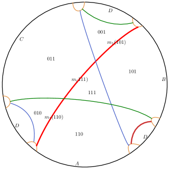
Figure 6: We choose $I_{1},I_{2},I_{3}$ as $AB,AC,BC$ as before. The bold red line is $\tilde{m}(AB)$, blue and green lines are $\tilde{m}(AC)$ and $\tilde{m}(BC)$ respectively. $\tilde{m}(AB)$ is cut into three parts by $\tilde{m}(AC)$ and $\tilde{m}(BC)$. We can see that $m_{1}(110)$, $m_{1}(111)$ and $m_{1}(101)$ are almost the same as $m(010,110)$, $m(011,111)$ and $m(001,101)$ respectively.

Theorem 2.

Only if $(x,x^{\prime})$ is directly connected can $m(x,x^{\prime})$ contribute nonzero area.

Proof.

According to Definition. 29, only $m_{l}(x)$ can contribute nonzero area and we have $\text{Area}[m(x,x^{\prime})]=\text{Area}[m_{l}(x)]$ if $(x,x^{\prime})$ is directly connected according to Lemma. 2. So only when $(x,x^{\prime})$ is directly connected can $m(x,x^{\prime})$ contribute nonzero area. ∎

Then we replace $m_{l}(x)$ with surface fragment $m(x,x^{\prime})$. Since all fragments of $\tilde{m}(I_{l}),l=1,\dots,L$ correspond to $(x,x^{\prime})$, only when $d(x,x^{\prime})=1$ might $m(x,x^{\prime})$ have nonzero contribution. We denote the set of all directly connected $(x,x^{\prime})$ by $\mathbb{A}$, which means that these surface fragments have nonzero area contribution. In other words, we have

$$\mathbb{A}\coloneqq\{(x,x^{\prime}):d(x,x^{\prime})=1\text{ and }x,x^{\prime}\in\mathbb{B}\}.$$ (31)

Theorem 3.

Direct connection is topological invariant under $\mathcal{T}$.

Proof.

We find that all $(x,x^{\prime})$ satisfying $\forall i\in[L]\setminus\{l\},x^{\prime}_{i}=x_{i}$ and $x^{\prime}_{l}\neq x_{l}$ will correspond to $(O_{\alpha}(x,l),O_{\beta}(x^{\prime},l))$ according to the definition of $O_{\alpha}(x,l)$ and $O_{\beta}(x,l)$ in Definition 29. And since the definition of $O_{\alpha}(x,l)$ and $O_{\beta}(x,l)$ is irrelevant to $x_{l}$, we should treat $(O_{\alpha}(x,l),O_{\beta}(x^{\prime},l))$ and $(O_{\alpha}(x^{\prime},l),O_{\beta}(x,l))$ as the same.

Then we can think that there is a map $\phi$ that $\phi(O_{\alpha}(x,l),O_{\beta}(x^{\prime},l))=(x,x^{\prime})$. We can easily verify that the map $\phi$ is well-defined and one-to-one if we treat $(x,x^{\prime})$ and $(x^{\prime},x)$ as the same. So directly connection is topological invariant under $\mathcal{T}$. ∎

Changing the systems’ position on $\partial M$ and occupied region does not change the structure of the topology $\mathcal{T}$. So the direct connection of $(x,x^{\prime})$ is irrelevant to systems’ position and occupied region.

Theorem 4.

For all $x,x^{\prime}\in\mathbb{B}$, $(x,x^{\prime})$ is connected.

Proof.

For all $x,x^{\prime}\in\mathbb{B}$, since $M^{\prime}$ is simply connected, there must be a path in $M^{\prime}$ that connects $\sigma(x)$ and $\sigma(x^{\prime})$ passing through some $\tilde{m}(I_{l})$. Each time when the path passes through a certain $\tilde{m}(I_{l})$, the bitstrings $x$ will change and only change the component $x_{l}$ once. As shown in Fig. 7, each bitstring $x$ is associated with a superscript $i$ whose value is arranged in order. Each time when the path gets through $\tilde{m}(I_{l})$, $x^{i}$ changes to $x^{i+1}$, i.e., the value of $i$ increases by one. In this way we get $x^{i}(i=1,\cdots,n)$ in proper order along the path and we let $x^{1}=x,x^{n}=x^{\prime}$. Therefore, $(x^{i},x^{i+1})(i=1,\cdots,n-1)$ is directly connected by definition. And thus, according to Definition. 3, $(x,x^{\prime})$ is connected. ∎

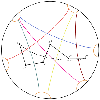
Figure 7: Polygonal line with arrow is the path that connect $\sigma(x^{1})$ and $\sigma(x^{6})$, and dotted line is the shortest (geometrical) path between the points of $\sigma(x^{1})$ and $\sigma(x^{6})$. We can easily find that $(x^{i},x^{i+1})$ is directly connected. The polygonal (black bold) line is the corresponding shortest weight path, which will pass through the $\tilde{m}(I_{l})$(color lines) when it moves from $\sigma(x^{i})$ to $\sigma(x^{i+1})$.

4.3 Find all $f(x)$ for nonempty bulk pieces

In previous subsections, we have shown how to exclude pairs with empty bulk pieces and surface fragments of zero-area contribution. Although by this way one can exclude most surface fragments, the situations for finding $f$ are still huge. Let us explain in the following. Before imposing the zero-area-contribution constraint, the number of allowed choices for $f(x)$ is $N(\mathbb{B})$ (same as the number of $x\in\mathbb{B}$), where $N(\mathbb{B})$ represents the total number of elements in $\mathbb{B}$. And the number of $f$’s inequality constraints is $N(\mathbb{A})$. Even though the number of inequality constraints is small enough, if we use an exhaustive method to find $f$, there is still $2^{R}$ possible $f(x)$ for each uncertain $x$. The number of uncertain $x$ is $N(\mathbb{B})-n$, where $n$ is the number of $f(x^{(i)})$ which has been fixed by the basic constraints (20). So the number of possible $f$ is $(2^{R})^{N(\mathbb{B})-n}$. In addition, we should verify $N(\mathbb{A})$ times at most for each possible $f$. Totally we need to verify $N(\mathbb{A})(2^{R})^{N(\mathbb{B})-n}$ times at most to find $f$. This is undoubtedly still huge. However, if we require that $f$ satisfying $d_{\beta}(f(x),f(x^{\prime}))\leq d_{\alpha}(x,x^{\prime})$ for all $x,x^{\prime}\in\mathbb{B}$, it turns out that one can find the possible $f(x)$ for some certain $x$ programmatically.

Our algorithm includes two parts. Firstly, let us denote the set of all possible $f(x)$ as $\mathcal{F}^{1}(x)$, then $\mathcal{F}^{1}(x^{(i)})=\{f(x^{(i)})\}$. Define $\mathbb{B}_{0}\coloneqq\bigcup_{i\in[n]}\{x^{(i)}\}$ and let $\mathbb{B}^{\prime}=\mathbb{B}_{0}$. See the detailed processes as follows:

• First step. Choose $x^{1}\in\mathbb{B}\setminus\mathbb{B}^{\prime}$, then find all possible $f(x^{1})\in\{0,1\}^{R}$ satisfying $d_{\alpha}(x^{1},x^{\prime})\geq d_{\beta}(f(x^{1}),f(x^{\prime}))$ for all $f(x^{\prime})\in\mathcal{F}^{1}(x^{\prime})$ of all $x^{\prime}\in\mathbb{B}^{\prime}$. Denote the set of all possible $f(x^{1})$ as $\mathcal{F}^{1}(x^{1})$, then add $x^{1}$ into $\mathbb{B}^{\prime}$, i.e. resetting $\mathbb{B}^{\prime}=\{x^{1}\}\cup\mathbb{B}^{\prime}$.

• Second step. Choose $x^{2}\in\mathbb{B}\setminus\mathbb{B}^{\prime}$, then find all possible $f(x^{2})\in\{0,1\}^{R}$ satisfying $d_{\alpha}(x^{2},x^{\prime})\geq d_{\beta}(f(x^{2}),f(x^{\prime}))$ for all $f(x^{\prime})\in\mathcal{F}^{1}(x^{\prime})$ of all $x^{\prime}\in\mathbb{B}^{\prime}$. Denote the set of all possible $f(x^{2})$ as $\mathcal{F}^{1}(x^{2})$, then add $x^{2}$ into $\mathbb{B}^{\prime}$, i.e. resetting $\mathbb{B}^{\prime}=\{x^{2}\}\cup\mathbb{B}^{\prime}$.

• ……

• $m^{\text{th}}$ step. Choose $x^{m}\in\mathbb{B}\setminus\mathbb{B}^{\prime}$, then find all possible $f(x^{m})\in\{0,1\}^{R}$ satisfying $d_{\alpha}(x^{m},x^{\prime})\geq d_{\beta}(f(x^{m}),f(x^{\prime}))$ for all $f(x^{\prime})\in\mathcal{F}^{1}(x^{\prime})$ of all $x^{\prime}\in\mathbb{B}^{\prime}$. Denote the set of all possible $f(x^{m})$ as $\mathcal{F}^{1}(x^{m})$, then add $x^{m}$ into $\mathbb{B}^{\prime}$, i.e. resetting $\mathbb{B}^{\prime}=\{x^{m}\}\cup\mathbb{B}^{\prime}$.

See Figure. 8 to help understanding the above steps intuitively.

If the number of possible $f(x)$ is large, we can narrow the range of $\mathcal{F}^{1}(x)$ by repeating the above steps with slight changes. Because there already have been $\mathcal{F}^{1}(x)$ for every $x$, we should consider $x^{\prime}\in\mathbb{B}$. And $x\in\mathbb{B}\setminus\mathbb{B}_{0}$ is also already numbered and does not need to be specified separately. Take $\forall x\in\mathbb{B}$ and $\mathcal{F}^{2}(x)=\mathcal{F}^{1}(x)$, then see the processes as follows:

• First step. Choose $x^{1}\in\mathbb{B}\setminus\mathbb{B}_{0}$, then find all possible $f(x^{1})\in\{0,1\}^{R}$ satisfying $d_{\alpha}(x^{1},x^{\prime})\geq d_{\beta}(f(x^{1}),f(x^{\prime}))$ for all $f(x^{\prime})\in\mathcal{F}^{2}(x^{\prime})$ of all $x^{\prime}\in\mathbb{B}\setminus\{x^{1}\}$. Then replace $\mathcal{F}^{2}(x^{1})$ with the set of all possible $f(x^{1})$ we just get.

• Second step. Choose $x^{2}\in\mathbb{B}\setminus\mathbb{B}_{0}$, then find all possible $f(x^{2})\in\{0,1\}^{R}$ satisfying $d_{\alpha}(x^{2},x^{\prime})\geq d_{\beta}(f(x^{2}),f(x^{\prime}))$ for all $f(x^{\prime})\in\mathcal{F}^{2}(x^{\prime})$ of all $x^{\prime}\in\mathbb{B}\setminus\{x^{2}\}$. Then replace $\mathcal{F}^{2}(x^{2})$ with the set of all possible $f(x^{2})$ we just get.

• ……

• $m^{\text{th}}$ step. Choose $x^{m}\in\mathbb{B}\setminus\mathbb{B}_{0}$, then find all possible $f(x^{m})\in\{0,1\}^{R}$ satisfying $d_{\alpha}(x^{m},x^{\prime})\geq d_{\beta}(f(x^{m}),f(x^{\prime}))$ for all $f(x^{\prime})\in\mathcal{F}^{2}(x^{\prime})$ of all $x^{\prime}\in\mathbb{B}\setminus\{x^{m}\}$. Then replace $\mathcal{F}^{2}(x^{m})$ with the set of all possible $f(x^{m})$ we just get.

One can repeat this process to get $\mathcal{F}^{n}(x)$ for all $x\in\mathbb{B}$. Since $\mathcal{F}^{n+1}(x)\subset\mathcal{F}^{n}(x)$, it means for $\forall x\in\mathbb{B}$, $\{\mathcal{F}^{n}(x)\}$ is a set sequence monotonically decreasing with $n$, where the number of elements of $\mathcal{F}^{n}(x)$ is finite. Then $\exists N,\forall n>N,\mathcal{F}^{n}(x)$ will no longer decrease as $n$ increases. We denote $\lim_{n\to\infty}\mathcal{F}^{n}(x)$ as $\mathcal{F}(x)$. $\mathcal{F}(x)$ is either a certain nonempty set or empty set.

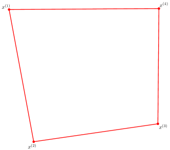
(a) Step 0

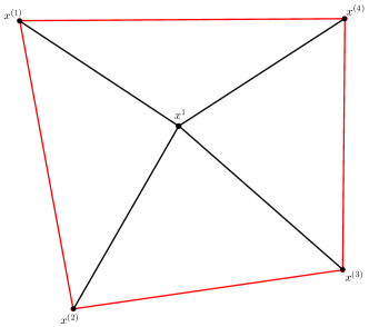
(b) Step 1

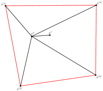
(c) Step 2

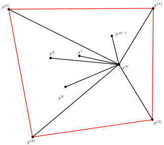
(d) Step m

Figure 8: There are fixed $f(x^{(i)})$ and uncertain $f(x^{j})$. Step 1, in Fig(b), we add $x^{1}$ and connect it with all appeared point, each connection satisfying $d_{\beta}\leq d_{\alpha}$(is short for $d_{\beta}(f(x),f(x^{\prime}))\leq d_{\alpha}(x,x^{\prime})$). Every step is the same as step 1, we add a point and connect it with all appeared points, each connection satisfying $d_{\beta}\leq d_{\alpha}$.

And if we first choose $x^{j}\in\mathbb{B}$ so that $d(x^{j},x^{(i)})=1$, then the number of possible $f(x^{j})$ may be less than the choice of the random $x^{j}\in\mathbb{B}$. The time complexity of the first part is of order $[N(\mathbb{B})]^{2}/2$ for the first process, while $[N(\mathbb{B})]^{2}$ for the later process. If we repeat the process $a$ times in total, then the whole time complexity of first part is of order $(2a-1)[N(\mathbb{B})]^{2}/2$.

Now let us turn to the second part. If for all $x\in\mathbb{B}$, we can find $f(x)\in\mathcal{F}(x)$ so that $f$ satisfies inequalities of weight distance constraints for all connected pairs $(x,x^{\prime})$, then this $f$ is what we want and thus we prove the inequality successfully. This is a global search whose time complexity is of order $\prod_{x\in\mathbb{B}}N(\mathcal{F}(x))$ ($N(\mathcal{F}(x))$ is the number of elements of $\mathcal{F}(x)$) which is huge. However, it can imply whether the inequality is compact or not. If $\prod_{x\in\mathbb{B}}N(\mathcal{F}(x))$ is huge, then we might find a large number of possible $f$, which means the constraints of weight distance inequality on $f$ could be tighter, i.e. the inequality that we prove might not be compact. So our method is still efficient for proving the compact inequality.

4.4 Case with the overlapping relative homologous surface

In this subsection let us focus on a special case where some relative homologous surfaces $\tilde{m}(I_{l})$ and $\tilde{m}(I_{l^{\prime}})$ are overlapping, as depicted in Fig. 9. In this case, there is a caveat that the Lemma 2 and Theorem 2 naively seem to be no longer valid, since now the geometrically neighboring regions are no longer directly connected as already mentioned in section 4.2. To rescue this case, our strategy is the following: we first suppose there is a nonempty small region $\sigma(\epsilon)$ between $\tilde{m}(I_{l})$ and $\tilde{m}(I_{l^{\prime}})$ by taking an infinitesimal transformation on $\tilde{m}(I_{l})$ and $\tilde{m}(I_{l^{\prime}})$ as shown in Fig. 9, such that $\text{Area}[\tilde{m}(I_{l})\cap\tilde{m}(I_{l}^{\prime})]$ is equal to $0$, so all previous procedures and theorems are valid. Then we can take a limit $\sigma(\epsilon)\rightarrow\emptyset$. Because infinitesimal change of the area of $\tilde{m}(I_{l})$ does not affect the method of finding $f$, the Lemma 2 and Theorem 2 are robust under this limit. Our method of finding $f$ is still valid even for the case with the overlapping relative homologous surface.

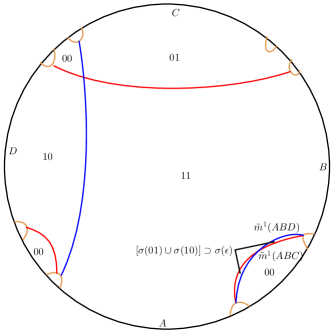
Figure 9: We take an infinitesimal transformation for $\tilde{m}(ABC)$ and $\tilde{m}(ABD)$ in figure (a), then we can get figure (b) so that $\sigma(\epsilon)\subset\sigma(01)\cup\sigma(10)$ and $\text{Area}[\tilde{m}(ABC)\cap\tilde{m}(ABD)]=0$.

5 Examples

By the definition of RHE, we expect the RHE possesses plentiful same inequalities as HEE. Related work DSZ also pointed out this from the “flow” perspective. While we will assume some inequalities of RHE and then prove these inequalities by using the above improved proof-by-contraction method from the “cut” perspective.

5.1 Strong Subadditivity (SSA)

We expect the SSA of RHE for a tripartite mixed state $\rho_{ABC}$, written as

$$\tilde{S}_{AC}+\tilde{S}_{BC}\geq\tilde{S}_{C}+\tilde{S}_{ABC}.$$ (32)

To prove this inequality, let us set $A_{1}=A,A_{2}=B,A_{3}=C,A_{4}=O$,$I_{1}=\{1,3\},I_{2}=\{2,3\}$,$J_{1}=\{3\},J_{2}=\{1,2,3\}$, $d_{\alpha}(x,x^{\prime})=\sum_{l=1}^{2}\absolutevalue*{x_{l}-x^{\prime}_{l}}$ and $d_{\beta}(f(x),f(x^{\prime}))=\sum_{r=1}^{2}\absolutevalue*{f(x)_{r}-f(x^{\prime})_{r}}$ Then basic constraints can be found in Table 1.

	$x^{(i)}$	$f(x^{(i)})$
1	10	01
2	01	01
3	11	11
4	00	00

Table 1: The basic constraints of $f(x)$ about SSA

Obviously all $x$ corresponds to a nonempty bulk piece, and all $f(x)$ are determined. It is easy to verify that $d_{\beta}(f(x),f(x^{\prime}))\leq d_{\alpha}(x,x^{\prime})$ for all directly connected $(x,x^{\prime})$. So the SSA of RHE is proved.

5.2 Monogamy of mutual information (MMI)

We assume the MMI of RHE for a tripartite mixed state $\rho_{ABC}$, as

$$\tilde{S}_{AB}+\tilde{S}_{AC}+\tilde{S}_{BC}\geq\tilde{S}_{A}+\tilde{S}_{B}+\tilde{S}_{C}+\tilde{S}_{ABC}.$$ (33)

To prove this, we set:
$A_{1}=A,A_{2}=B,A_{3}=C,A_{4}=O$,
$I_{1}=\{1,2\},I_{2}=\{1,3\},I_{3}=\{2,3\}$,
$J_{1}=\{1\},J_{2}=\{2\},J_{3}=\{3\},J_{4}=\{1,2,3\}$,
$d_{\alpha}(x,x^{\prime})=\sum_{l=1}^{3}\absolutevalue*{x_{l}-x^{\prime}_{l}}$, $d_{\beta}(f(x),f(x^{\prime}))=\sum_{r=1}^{4}\absolutevalue*{f(x)_{r}-f(x^{\prime})_{r}}.$

Basic constraints can be found in Table 2.

	$x^{(i)}$	$f(x^{(i)})$
1	110	1001
2	101	0101
3	011	0011
4	000	0000

Table 2: The basic constraints of $f(x)$ about MMI

First, find all nonempty bulk pieces. We find other $x$ expect $x^{(i)}$ also corresponds to nonempty bulk piece.We get $\mathbb{B}\setminus\left(\bigcup_{i\in[4]}\{x^{(i)}\}\right)=\{100,010,001,111\}$.

Then, choose $x^{1}=100$, find all $f(x^{1})$ satisfying $d_{\beta}(f(x^{(i)}),f(x^{1}))\leq d_{\alpha}(x^{(i)},x^{1})$, we get $\mathcal{F}(x^{1})=\{0001\}$.
Choose $x^{2}=010$ find all $f(x^{1})$ satisfying $d_{\beta}(f(x^{(i)}),f(x^{2}))\leq d_{\alpha}(x^{(i)},x^{2})$ and $d_{\beta}(f(x),f(x_{2}))\leq d_{\alpha}(x,x^{2}),f(x)\in\mathcal{F}(x^{1})$, we get $\mathcal{F}(x^{2})=\{0001\}$.
Choose $x^{3}=001$, find all $f(x^{3})$ satisfying$d_{\beta}(f(x^{(i)}),f(x^{3}))\leq d_{\alpha}(x^{(i)},x^{3})$ and $d_{\beta}(f(x),f(x^{3}))\leq d_{\alpha}(x,x^{3}),f(x)\in\bigcup_{j\in[2]}\mathcal{F}(x^{j})$, we get $\mathcal{F}(x^{2})=\{0001\}$.
Choose $x^{4}=111$, find all $f(x^{4})$ satisfying$d_{\beta}(f(x^{(i)}),f(x^{4}))\leq d_{\alpha}(x^{(i)},x^{4})$ and $d_{\beta}(f(x),f(x^{4}))\leq d_{\alpha}(x,x^{4}),f(x)\in\bigcup_{j\in[3]}\mathcal{F}(x^{j})$, we get $\mathcal{F}(x^{4})=\{0001\}$. We have found all $f(x)$, and we can verify that $d_{\beta}\leq d_{\alpha}$ for all directly connected $(x,x^{\prime})$, so we prove the MMI of RHE.

5.3 Inequality of four regions

The above two examples correspond to three regions. Actually, our approach is valid for more regions. This is a concrete example for four regions. Before proceeding, let us recall that the inequality of HEE was discovered by Bao:2015bfa for a quadripartite mixed state $\rho_{ABCD}$ as follows:

$$I(A:B|C)+I(A:B|D)+I(C:D)\geq I(A:B)$$ (34)

where $I(A:B)$ is the mutual information defined as $I(A:B)\coloneqq S_{A}+S_{B}-S_{AB}$ and $I(A:B|C)$ is the conditional mutual information defined as $I(A:B|C)\coloneqq S_{AC}+S_{BC}-S_{C}-S_{ABC}$. Now we can transform the above formula of HEE into the following form in terms of RHE:

$$\tilde{S}_{AB}+\tilde{S}_{AC}+\tilde{S}_{AD}+\tilde{S}_{BC}+\tilde{S}_{BD}\geq\tilde{S}_{A}+\tilde{S}_{B}+\tilde{S}_{CD}+\tilde{S}_{ABC}+\tilde{S}_{ABD}.$$ (35)

To prove this, we set:
$A_{1}=A,A_{2}=B,A_{3}=C,A_{4}=D,A_{5}=O$,
$I_{1}=\{1,2\},I_{2}=\{1,3\},I_{3}=\{1,4\},I_{4}=\{2,3\},I_{5}=\{2,4\}$,
$J_{1}=\{1\},J_{2}=\{2\},J_{3}=\{3,4\},J_{4}=\{1,2,3\},J_{5}=\{1,2,4\}$,
$d_{\alpha}(x,x^{\prime})=\sum_{l=1}^{5}\absolutevalue*{x_{l}-x^{\prime}_{l}}$
$d_{\beta}(f(x),f(x^{\prime}))=\sum_{r=1}^{5}\absolutevalue*{f(x)_{r}-f(x^{\prime})_{r}}.$

Basic constraints can be found in Table 3.

	$x^{(i)}$	$f(x^{(i)})$
1	11100	10011
2	10011	01011
3	01010	00110
4	00101	00101
5	00000	00000

Table 3: The basic constraints of $f$ about the inequality of four regions

First, find all nonempty bulk pieces. We find other $x$ expect $x^{(i)}$ also corresponds to nonempty bulk piece. Then for all $x^{j}\in\mathbb{B}\setminus\left(\bigcup_{i\in[5]}\{x^{(i)}\}\right)$, we find possible $f(x^{j})$ by following the steps we’ve introduced in section 4.3. We program to calculate the result of $f(x)$ in Table 4.

$x$	$f(x)$	$x$	$f(x)$
11010	00010	00100	00001
11000	10010	00011	00011
10101	00111	00010	00010
10100	00011	00001	00001
10010	01010	00000	00000
10001	00011	11100	10011
10000	00010	10011	01011
01100	00011	01010	00110
01000	00010	00101	00101

Table 4: $f(x)$ of all $x\in\mathbb{B}$, bold numbers are the basic constraints of $f$

We’ve already got all $f(x)$, and we can verify that $d_{\beta}\leq d_{\alpha}$ for all directly connected $(x,x^{\prime})$, so we prove this inequality of RHE.

5.4 Inequality of five regions

An inequality of HEE that is discovered by HEC2 , then we expect the same inequality of RHE for a 5-partite mixed state $\rho_{ABCDE}$ as follows:

$$\tilde{S}_{ABC}+\tilde{S}_{ABD}+\tilde{S}_{ACE}+\tilde{S}_{BDE}+\tilde{S}_{CDE}\geq\tilde{S}_{AB}+\tilde{S}_{AC}+\tilde{S}_{BD}+\tilde{S}_{CE}+\tilde{S}_{DE}+\tilde{S}_{ABCDE}.$$ (36)

To prove this, we set:
$A_{1}=A,A_{2}=B,A_{3}=C,A_{4}=D,A_{5}=E,A_{6}=O$,
$I_{1}=\{1,2,3\},I_{2}=\{1,2,4\},I_{3}=\{1,3,5\},I_{4}=\{2,4,5\},I_{5}=\{3,4,5\}$,
$J_{1}=\{1,2\},J_{2}=\{1,3\},J_{3}=\{2,4\},J_{4}=\{3,5\},J_{5}=\{4,5\},J_{6}=\{1,2,3,4,5\}$,
$d_{\alpha}(x,x^{\prime})=\sum_{l=1}^{5}\absolutevalue*{x_{l}-x^{\prime}_{l}}$,$d_{\beta}(f(x),f(x^{\prime}))=\sum_{r=1}^{6}\absolutevalue*{f(x)_{r}-f(x^{\prime})_{r}}.$

Basic constraints can be found in Table 5.

	$x^{(i)}$	$f(x^{(i)})$
1	11100	110001
2	11010	101001
3	10101	010101
4	01011	001011
5	00111	000111
6	00000	000000

Table 5: The basic constraints of $f$ about the inequality of five regions

First, find all nonempty bulk pieces. We find other $x$ expect $x^{(i)}$ also corresponds to nonempty bulk piece. Then for all $x^{j}\in\mathbb{B}\setminus\left(\bigcup_{i\in[6]}\{x^{(i)}\}\right)$, we find possible $f(x^{j})$ by following the steps we have introduced in section 4.3. We program to calculate the result of $f(x)$ in Table 6.

$x$	$f(x)$	$x$	$f(x)$	$x$	$f(x)$	$x$	$f(x)$
11111	000001	01111	000011	10111	000101	01000	000001
11110	100001	01110	000001	10110	000001	00110	000101
11101	010001	01101	000001	10100	010001	00101	000101
11011	001001	01100	100001	10011	000001	00100	000001
11001	000001	01010	001001	10010	100001	00011	000011
11000	100001	01001	001001	11100	110001	11010	101001
10000	000001	00001	000001	10101	010101	01011	001011
10001	010001	00010	000001	00111	000111	00000	000000

Table 6: $f(x)$ of all $x\in\mathbb{B}$, bold numbers are the basic constraints of $f$

We’ve found $f$ for all $x\in\mathbb{B}$, we can verify that $d_{\beta}\leq d_{\alpha}$ for all directly connected $(x,x^{\prime})$, so we prove the inequality.

6 Conclusion and Discussion

In this work, we systematically study the proof-by-contraction method, an important technique developed for proving a given holographic entropy inequality so as to fix HEC of a system. This method includes a contraction map $f$, which plays a central role in this method and is of particular difficulty to construct for more-region ($n\geq 4$) cases. Here we develop, based on a pioneer work Bao:2015bfa ; Akers:2021lms , a general and effective rule to rule out most of the cases such that $f$ can be obtained in a relatively simple way and can be processed by computer programming. We achieve this by carefully investigating all possible constraints imposed on $f$, the basic constraints and constraints of inequality of weight distance, which is not fully developed in the original method. Compared with the original method proposed in Bao:2015bfa , our method has two obvious improvements. Firstly, the time complexity of first part of our algorithm is of order $[N(\mathbb{B})]^{2}$, which is less than the order $(2^{L})^{2}$ of the algorithm in Bao:2015bfa . The second part is a global search for $f$. Secondly, our algorithm is globally optimal rather than locally optimal, implying that more possible $f$ can be found. And since we only consider $x\in\mathbb{B}$ instead of $x\in\{0,1\}^{L}$, the constraints on $f$ is less than the greedy algorithm Bao:2015bfa , thus again more possible $f$ can be found. So that our method can be used to prove some possible inequalities that the method in Bao:2015bfa can not. The validity of our method has been confirmed by several examples. Thus our method can be used to confirm the authenticity of some unproved inequality. It also can shed light on finding new inequalities of HEE.

On the other hand, we consider the concept of RHE in static slice by the notion of relative homology Headrick:2017ucz , which is a generalization of holographic entanglement entropy that is suitable for characterizing the entanglement of mixed states. The holographic entanglement entropy and entanglement wedge cross section $E_{W}$ are two particular cases of RHE DCS ; HHea . In this paper, we extend the whole framework of proof-by-contraction to RHE. We find that our method not only can be used to prove the inequalities of HEE, but also can be used to prove the inequalities of $E_{W}$.

As a future direction, the completeness of our method is of great interest. There are three aspects that will affect the completeness of the method. The first and the most important is, as mentioned in section 3.4, that the weight distance inequalities $d_{\alpha}(x,x^{\prime})\geq d_{\beta}(f(x),f(x^{\prime}))$ for all bitstrings pairs encoded by the surface fragments with non-zero area contribution is simply a sufficient condition for inequality (10). The necessity of the condition is still unproven partially because we cannot find, even for the MMI, the case where the area of a certain surface fragment becomes dominant among the area of all other surface fragments. Second, some $x\in\mathbb{B}$ might correspond to empty bulk pieces, so there might exist unnecessary constraints on $f$. Third, we require the weight distance inequality for $(x,x^{\prime}):\forall x,x^{\prime}\in\mathbb{B}$, so there also exist unnecessary constraints on $f$. We leave these for future work.

Another future direction worthy of mention is to generalize our method to prove the inequalities of RHE in the covariant case, as we focus on the static case in the paper. It was known that the SA, SSA and MMI of HEE can be proved to hold in the covariant case by Wall’s “maximin” method with assumed null curvature condition EW2 , but this method encounters obstacles for the inequalities beyond the MMI Rota:2017ubr ; HEC1 . So it is natural to think whether the RHE will encounter similar troubles. Unfortunately, as far as we know, the definition of the RHE in Headrick:2017ucz was mainly set in the static case so far by using the max flow-min cut theorem, and the general covariant RHE remains to be studied. One may expect that the general covariant RHE can be realized with the help of analogous min flow-max cut theorem in the Lorentzian setting Headrick:2017ucz , as done for the holographic complexity Pedraza:2021mkh ; Pedraza:2021fgp . However, the main difference between RHE and HEE is that, the RHE possesses a more general homology condition than HEE. We expect the RHE will encounter similar troubles like HEE in principle when we try to prove inequalities in the covariant case, as HEE itself can also be regarded as a special case of RHE. It remains to be further clarified in the future.

- (1) J. M. Maldacena, “The Large N limit of superconformal field theories and supergravity,” Int. J. Theor. Phys. 38, 1113 (1999) [Adv. Theor. Math. Phys. 2, 231 (1998)] [hep-th/9711200].
- (2) E. Witten, “Anti-de Sitter space and holography,” Adv. Theor. Math. Phys. 2, 253 (1998) [hep-th/9802150].
- (3) S. S. Gubser, I. R. Klebanov and A. M. Polyakov, “Gauge theory correlators from noncritical string theory,” Phys. Lett. B 428, 105 (1998) [hep-th/9802109].
- (4) S. Ryu and T. Takayanagi, “Holographic derivation of entanglement entropy from AdS/CFT,” Phys. Rev. Lett. 96, 181602 (2006), arXiv:hep-th/0603001.
- (5) V. E. Hubeny, M. Rangamani and T. Takayanagi, “A Covariant holographic entanglement entropy proposal,” JHEP 0707, 062 (2007), arXiv:0705.0016 [hep-th].
- (6) I. Heemskerk, J. Penedones, J. Polchinski and J. Sully, “Holography from Conformal Field Theory,” JHEP 10, 079 (2009) [arXiv:0907.0151 [hep-th]].
- (7) N. Bao, S. Nezami, H. Ooguri, B. Stoica, J. Sully and M. Walter, “The Holographic Entropy Cone,” JHEP 09, 130 (2015) [arXiv:1505.07839 [hep-th]].
- (8) N. Bao and M. Mezei, “On the Entropy Cone for Large Regions at Late Times,” arXiv:1811.00019 [hep-th].
- (9) S. Hernández Cuenca, “Holographic entropy cone for five regions,” Phys. Rev. D 100, no.2, 026004 (2019) arXiv:1903.09148 [hep-th].
- (10) B. Czech and X. Dong, “Holographic Entropy Cone with Time Dependence in Two Dimensions,” JHEP 10, 177 (2019), arXiv:1905.03787 [hep-th].
- (11) N. Bao, N. Cheng, S. Hernández-Cuenca and V. P. Su, “The Quantum Entropy Cone of Hypergraphs,” SciPost Phys. 9, no.5, 5 (2020) [arXiv:2002.05317 [quant-ph]].
- (12) M. Walter and F. Witteveen, “Hypergraph min-cuts from quantum entropies,” J. Math. Phys. 62, no.9, 092203 (2021) [arXiv:2002.12397 [quant-ph]].
- (13) N. Bao, N. Cheng, S. Hernández-Cuenca and V. P. Su, “A Gap Between the Hypergraph and Stabilizer Entropy Cones,” arXiv:2006.16292 [quant-ph].
- (14) M. Rota and S. J. Weinberg, “New constraints for holographic entropy from maximin: A no-go theorem,” Phys. Rev. D 97, no.8, 086013 (2018) [arXiv:1712.10004 [hep-th]].
- (15) D. Avis and S. Hernández-Cuenca, “On the foundations and extremal structure of the holographic entropy cone,” [arXiv:2102.07535 [math.CO]].
- (16) C. Akers, S. Hernández-Cuenca and P. Rath, “Quantum Extremal Surfaces and the Holographic Entropy Cone,” JHEP 11, 177 (2021) [arXiv:2108.07280 [hep-th]].
- (17) M. Headrick and V. E. Hubeny, “Riemannian and Lorentzian flow-cut theorems,” Class. Quant. Grav. 35, no.10, 10 (2018) [arXiv:1710.09516 [hep-th]].
- (18) M. Freedman and M. Headrick, “Bit threads and holographic entanglement,” Commun. Math. Phys. 352, no. 1, 407 (2017), arXiv:1604.00354[hep-th].
- (19) B. M. Terhal, M. Horodecki, D. W. Leung and D. P. DiVincenzo, “The entanglement of purification,” J. Math. Phys. 43 (2002) 4286, arXiv:quant-ph/0202044.
- (20) K. Umemoto and T. Takayanagi, “Entanglement of purification through holographic duality,” Nature Phys. 14, no. 6, 573 (2018), arXiv:1708.09393 [hep-th].
- (21) P. Nguyen, T. Devakul, M. G. Halbasch, M. P. Zaletel and B. Swingle, “Entanglement of purification: from spin chains to holography,” JHEP 1801, 098 (2018), arXiv:1709.07424 [hep-th].
- (22) B. Czech, J. L. Karczmarek, F. Nogueira and M. Van Raamsdonk, “The Gravity Dual of a Density Matrix,” Class. Quant. Grav. 29 (2012) 155009, arXiv:1204.1330 [hep-th].
- (23) A. C. Wall, “Maximin Surfaces, and the Strong Subadditivity of the Covariant Holographic Entanglement Entropy,” Class. Quant. Grav. 31 (2014) no.22, 225007, arXiv:1211.3494 [hep-th].
- (24) M. Headrick, V. E. Hubeny, A. Lawrence and M. Rangamani, “Causality and holographic entanglement entropy,” JHEP 1412 (2014) 162, arXiv:1408.6300 [hep-th].
- (25) N. Bao and I. F. Halpern, “Holographic Inequalities and Entanglement of Purification,” JHEP 1803, 006 (2018), arXiv:1710.07643 [hep-th].
- (26) A. Bhattacharyya, T. Takayanagi and K. Umemoto, “Entanglement of Purification in Free Scalar Field Theories,” JHEP 1804, 132 (2018), arXiv:1802.09545 [hep-th].
- (27) D. Blanco, M. Leston and G. Pérez-Nadal, “Gravity from entanglement for boundary subregions,” JHEP 0618, 130 (2018), arXiv:1803.01874 [hep-th].
- (28) H. Hirai, K. Tamaoka and T. Yokoya, “Towards Entanglement of Purification for Conformal Field Theories,” PTEP 2018, no. 6, 063B03 (2018), arXiv:1803.10539 [hep-th].
- (29) R. Espíndola, A. Guijosa and J. F. Pedraza, “Entanglement Wedge Reconstruction and Entanglement of Purification,” Eur. Phys. J. C 78, no. 8, 646 (2018), arXiv:1804.05855 [hep-th].
- (30) N. Bao and I. F. Halpern, “Conditional and Multipartite Entanglements of Purification and Holography,” Phys. Rev. D 99, no. 4, 046010 (2019), arXiv:1805.00476 [hep-th].
- (31) Y. Nomura, P. Rath and N. Salzetta, “Pulling the Boundary into the Bulk,” Phys. Rev. D 98, no. 2, 026010 (2018), arXiv:1805.00523 [hep-th].
- (32) K. Umemoto and Y. Zhou, “Entanglement of Purification for Multipartite States and its Holographic Dual,” JHEP 1810, 152 (2018), arXiv:1805.02625 [hep-th].
- (33) R. Abt, J. Erdmenger, M. Gerbershagen, C. M. Melby-Thompson and C. Northe, “Holographic Subregion Complexity from Kinematic Space,” JHEP 1901, 012 (2019), arXiv:1805.10298 [hep-th].
- (34) A. May and E. Hijano, “The holographic entropy zoo,” JHEP 1810, 036 (2018), arXiv:1806.06077 [hep-th].
- (35) Y. Chen, X. Dong, A. Lewkowycz and X. L. Qi, “Modular Flow as a Disentangler,” JHEP 1812, 083 (2018), arXiv:1806.09622 [hep-th].
- (36) J. Kudler-Flam and S. Ryu, “Entanglement negativity and minimal entanglement wedge cross sections in holographic theories,” arXiv:1808.00446 [hep-th].
- (37) K. Tamaoka, “Entanglement Wedge Cross Section from the Dual Density Matrix,” Phys. Rev. Lett. 122, no. 14, 141601 (2019), [arXiv:1809.09109 [hep-th]].
- (38) J. C. Cresswell, I. T. Jardine and A. W. Peet, “Holographic relations for OPE blocks in excited states,” JHEP 1903, 058 (2019), arXiv:1809.09107 [hep-th].
- (39) E. Caceres and M. L. Xiao, “Complexity-action of subregions with corners,” JHEP 1903, 062 (2019), arXiv:1809.09356 [hep-th].
- (40) R. Q. Yang, C. Y. Zhang and W. M. Li, “Holographic entanglement of purification for thermofield double states and thermal quench,” JHEP 1901, 114 (2019), arXiv:1810.00420 [hep-th].
- (41) N. Bao, A. Chatwin-Davies and G. N. Remmen, “Entanglement of Purification and Multiboundary Wormhole Geometries,” JHEP 1902, 110 (2019), arXiv:1811.01983 [hep-th].
- (42) N. Bao, “Minimal Purifications, Wormhole Geometries, and the Complexity=Action Proposal,” arXiv:1811.03113 [hep-th].
- (43) N. Bao, G. Penington, J. Sorce and A. C. Wall, “Beyond Toy Models: Distilling Tensor Networks in Full AdS/CFT,” arXiv:1812.01171 [hep-th].
- (44) P. Caputa, M. Miyaji, T. Takayanagi and K. Umemoto, “Holographic Entanglement of Purification from Conformal Field Theories,” Phys. Rev. Lett. 122, no. 11, 111601 (2019), arXiv:1812.05268 [hep-th].
- (45) W. Z. Guo, “Entanglement of Purification and Projective Measurement in CFT,” arXiv:1901.00330 [hep-th].
- (46) P. Liu, Y. Ling, C. Niu and J. P. Wu, “Entanglement of Purification in Holographic Systems,” arXiv:1902.02243 [hep-th].
- (47) A. Bhattacharyya, A. Jahn, T. Takayanagi and K. Umemoto, “Entanglement of Purification in Many Body Systems and Symmetry Breaking,” arXiv:1902.02369 [hep-th].
- (48) M. Ghodrati, X. M. Kuang, B. Wang, C. Y. Zhang and Y. T. Zhou, “The connection between holographic entanglement and complexity of purification,” arXiv:1902.02475 [hep-th].
- (49) J. Kudler-Flam, I. MacCormack and S. Ryu, “Holographic entanglement contour, bit threads, and the entanglement tsunami,” arXiv:1902.04654 [hep-th].
- (50) K. Babaei Velni, M. R. Mohammadi Mozaffar and M. H. Vahidinia, “Some Aspects of Holographic Entanglement of Purification,” arXiv:1903.08490 [hep-th].
- (51) J. Harper, M. Headrick and A. Rolph, “Bit Threads in Higher Curvature Gravity,” JHEP 1811, 168 (2018), arXiv:1807.04294 [hep-th].
- (52) S. X. Cui, P. Hayden, T. He, M. Headrick, B. Stoica and M. Walter, “Bit Threads and Holographic Monogamy,” arXiv:1808.05234 [hep-th].
- (53) V. E. Hubeny, “Bulk locality and cooperative flows,” JHEP 1812, 068 (2018), arXiv:1808.05313 [hep-th].
- (54) C. A. Agón, J. De Boer and J. F. Pedraza, JHEP 05, 075 (2019) [arXiv:1811.08879 [hep-th]].
- (55) D. H. Du, C. B. Chen and F. W. Shu, “Bit threads and holographic entanglement of purification,” JHEP 1908, 140 (2019), arXiv:1904.06871 [hep-th].
- (56) J. Harper and M. Headrick, “Bit threads and holographic entanglement of purification,” JHEP 1908, 101 (2019), arXiv:1906.05970 [hep-th].
- (57) D. H. Du, F. W. Shu and K. X. Zhu, “Inequalities of Holographic Entanglement of Purification from Bit Threads,” Eur. Phys. J. C 80, no.8, 700 (2020) [arXiv:1912.00557 [hep-th]].
- (58) C. A. Agón and J. F. Pedraza, “Quantum bit threads and holographic entanglement,” JHEP 02 (2022), 180 [arXiv:2105.08063 [hep-th]].
- (59) J. F. Pedraza, A. Russo, A. Svesko and Z. Weller-Davies, “Lorentzian Threads as Gatelines and Holographic Complexity,” Phys. Rev. Lett. 127, no.27, 271602 (2021) [arXiv:2105.12735 [hep-th]].
- (60) J. F. Pedraza, A. Russo, A. Svesko and Z. Weller-Davies, “Sewing spacetime with Lorentzian threads: complexity and the emergence of time in quantum gravity,” JHEP 02, 093 (2022) [arXiv:2106.12585 [hep-th]].