claimClaim remarkRemark hypothesisHypothesis

Optimization Models and Interpretations for Three Types of Adversarial Perturbations against Support Vector MachinesW. Su, Q. Li and C. Cui






Optimization Models and Interpretations for Three Types of Adversarial Perturbations against Support Vector Machines



Wen Su
School of Mathematics and Statistics, Beijing Institute of Technology, Beijing, 100081, China ().
suwen019@163.com

  
Qingna Li
School of Mathematics and Statistics, Beijing Key Laboratory on MCAACI/Key Laboratory of Mathematical Theory and Computation in Information Security, Beijing Institute of Technology, Beijing, 100081, China ().
qnl@bit.edu.cn

  
Chunfeng Cui
Corresponding author. LMIB of the Ministry of Education, School of Mathematical Sciences, Beihang University, Beijing, 100191, China ().
chunfengcui@buaa.edu.cn




Abstract
Adversarial perturbations have drawn great attentions in various deep neural networks. Most of them are computed by iterations and cannot be interpreted very well. In contrast, little attentions are paid to basic machine learning models such as support vector machines. In this paper, we investigate the optimization models and the interpretations for three types of adversarial perturbations against support vector machines, including sample-adversarial perturbations (sAP), class-universal adversarial perturbations (cuAP) as well as universal adversarial perturbations (uAP). For linear binary/multi classification support vector machines (SVMs), we derive the explicit solutions for sAP, cuAP and uAP (binary case), and approximate solution for uAP of multi-classification. We also obtain the upper bound of fooling rate for uAP. Such results not only increase the interpretability of the three adversarial perturbations, but also provide great convenience in computation since iterative process can be avoided. Numerical results show that our method is fast and effective in calculating three types of adversarial perturbations.


keywords: 
adversarial perturbation, universal adversarial perturbation, class-universal adversarial perturbation, support vector machines



90C25, 90C59, 68T45, 68T15





1 Introduction


Machine learning has proved to be a powerful tool in analyzing data from different applications, such as computer vision [16], natural language processing [33], speech recognition [13], recommendation system [1, 25, 26], cyber security [7, 35], clustering [4, 29] and so on.
However, some hackers can analyze the loopholes in machine learning to launch attacks on intelligent applications. The attackers can fool the trained machine learning system by designing input data.
For example, in a spam detection system, attackers can confuse the machine learning detection system by adding unrelated tokens to their emails [14]. Correspondingly, some researchers also modify neural network structure to make it resist attacks [30].
The security of machine learning systems is still an important research topic. Meanwhile, how to propose effective methods to calculate adversarial perturbations and how to make interpretation are getting more and more attentions. Due to the importance of adversarial perturbations, many researchers started to investigate the small pertubations to a machine learning system. It can be divided into three types: perturbations for a given sample (sAP), universal adversarial perturbations (uAP) and class-universal adversarial perturbations (cuAP). Below we discuss them one by one.


sAP is one of the most important and widely used types of adversarial perturbations. It has been studied in deep neural networks since 2014, and there are many methods to calculate sAP. Szegedy et al. [28] firstly discovered a surprising weakness of neural networks in the background of image classification, that is, neural networks are easily attacked by very small adversarial perturbations. Different from the previous input data designed by the attacker, these adversarial instances are almost indistinguishable from natural data (which means in human observation, there is no difference between adversarial instances and undisturbed input), and are misclassified by the neural network. This leads to researchers’ interest in studying sAP. Szegedy et al. [28] believed that the highly nonlinear nature of neural networks led to the existence of adversarial instances. However, Goodfellow et al. [12] put forward the opposite view. They believed that the linear behavior of neural networks in high-dimensional space is the real reason for the existence of adversarial instances.
The method (namely Fast Gradient Sign Method (FGSM)) proposed in [12] is designed based on gradient and has also become one of the mainstream method.
[20] and [17] further improved FGSM, which normalized the gradient formula calculated by FGSM using $l_{2}\mbox{-}$norm and $l_{\infty}\mbox{-}$norm respectively. Different from the above methods, DeepFool is an attack method based on linearization and separating hyperplane [22], which initializes with the clean image that is assumed to reside in a region confined by the decision boundaries of the classifier. At each iteration, DeepFool perturbs the image by a small vector that takes the resulting image to the linearizing boundaries of the region within which the image resides.


As for uAP, it is another popular type of adversarial perturbations. uAP can be generated in advance and then applied dynamically during the attack. Moosavi-Dezfooli et al. [21] proposed a single small image perturbation that fools a state-of-the-art deep neural network classifier on all natural images. Such perturbations are dubbed universal, as they are imageagnostic. The fooling rate is the most widely adopted metric for evaluating the efficacy of uAP. Specifically, the fooling rate is defined as the percentage of samples whose prediction changes after uAP is applied, i.e., $\dfrac{\text{The number of }\hat{k}(x+r)\neq\hat{k}(x),x\in A}{\text{The number of data in }A}$, where $A$ is a given dataset and $\hat{k}$ is the known classifier.
The existence of uAP reveals the important geometric correlations among the high-dimensional decision boundary of classifiers. Since [21], many methods have been introduced by researchers to generate uAP, both data-driven and data-independent. Miyato et al. [24]
proposed a data-driven method. They generated uAP by using fooling and diversity objectives along with a generative model.
Cui et al. [8] investigated generating uAP by the active-subspace. Miyato et al. [23] proposed a data-independent method to generate uAP by fooling the features learned at multiple layers of the network.
Their method didn’t use any information about the training data distribution of the classifier.


In terms of cuAP, it is a modified uAP based on different applications.
It can attack the data in a class-discriminative way, which is more stealthy. As far as we known, less work has been done on cuAP, compared with sAP and uAP.
Zhang et al. [34] noticed that uAP might cause obvious misconduct, and it might make the users suspicious. Thus, they proposed CD-UAP (class discriminative universal adversarial perturbation). CD-UAP only attacks data from a chosen group of classes, while having limited the impact on the remaining classes. Since the classifier will only misbehave when the specific data from a targeted class is encountered, cuAP will not raise obvious suspicion. Ben et al. [2] extended cuAP to a targeted version, which means they made a perturbation to fool data of the particular class toward the targeted class they pre-defined.


Recently, some researchers turn their attentions to perturbations against SVM. Fawzi et al. [10] initiated the research on sAP against SVM, which provides more insights for the relationship between robustness and design parameters. Langenberg et al. [18] analyzed and quantified the numerical experiments of sAP on SVM, showing that the robustness of SVM is significantly affected by parameters which change the linearity of the models. However, there is no mathematical derivation of sAP on SVM.


In this paper, we systematically study the optimization models and the interpretations for three types of adversarial perturbations (sAP, cuAP and uAP) against classification models trained by SVMs. Inspired by the idea and framework in Deepfool [22], we propose the optimization models for sAP, cuAP and uAP against the trained SVMs and derive the explicit formulations for sAP, cuAP and uAP (binary case), and approximate formulation for uAP of multi-classification. For uAP, we provide an upper bound for the fooling rate. Our numerical results also verify the fast speed in finding the three types of adversarial perturbations for classification models.
The contributions of this paper are as follows. Firstly, we propose optimization models of sAP, cuAP and uAP against linear SVMs. Secondly, we derive the explicit solutions and the approximate solution for the three types of adversarial perturbations, avoiding iterative process.
Based on the formulae, we increase the interpretability of against SVM classification models.


The rest of the paper is organized as follows. In Section 2, we briefly review the binary and multiclass linear SVMs.
Then we propose a general optimization framework for adversarial perturbations of linear SVMs.
In Section 3 and Section 4, we solve sAP, cuAP and uAP for binary SVM and multiclass SVM, respectively.
In Section 5, we conduct numerical experiments on MNIST and CIFAR-10 dataset. Final conclusions are given in Section 6.



2 Optimization Models for Adversarial Perturbations against Linear SVMs



2.1 Training models of linear SVMs


In this part, we briefly review the optimization models of binary linear SVMs and multiclass linear SVMs.
We use the short-hand notation $[B]$ to denote the set $[B]=\{1,2,\dots,B\}$ for some integer $B\in\mathbb{N}$.
For the binary classification problem, we assume that the training dataset $D=\{(x_{1},y_{1}),(x_{2},y_{2}),\dots,(x_{n},y_{n})\}$ is given, with $x_{i}\in\mathbb{R}^{p}$ and $y_{i}\in\{-1,1\}$ is the label of the corresponding $x_{i}$. SVM aims to find the hyperplane $H\triangleq\{x:w^{\top}x+b=0\}$ such that the training data in $D$ are separated as much as possible. A typical soft-margin training model of the binary SVMs is the $L_{1}\mbox{-}$loss SVM model [5], which is given as follows



(1)

$$\min_{w\in\mathbb{R}^{p},\,b\in\mathbb{R},\,\xi\in\mathbb{R}^{n}}
\quad\frac{1}{2}||w||^{2}+C\sum_{i=1}^{n}\xi_{i}$$





s.t.
$$\quad y_{i}(w^{\top}x_{i}+b)\geq 1-\xi_{i},{i\in[n],}$$





$$\quad\xi_{i}\geq 0,{i\in[n]}.$$




Let $(w^{*},b^{*})\in\mathbb{R}^{p}\times\mathbb{R}$ be the solution obtained by solving the $L_{1}\mbox{-}$loss SVM Eq. 1. We show the separating hyperplane (decision boundary) in Fig. 1.
For a test sample $x\in\mathbb{R}^{p}$, the decision function is given by



(2)

$$\hat{k}(x)=sign(({w^{*}})^{\top}x+b^{*}).$$



We refer to [27] for other binary SVM models with different loss functions.


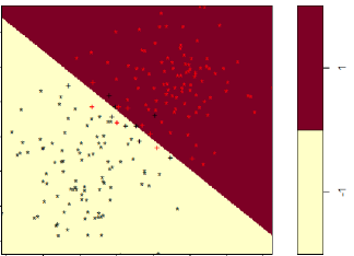
Figure 1: The decision boundary of binary linear SVM, ‘$*$’ indicates data points, and ‘$+$’ indicates support vectors.


In terms of multiclass linear SVMs, we assume that the training dataset is given by $D=\{(x_{1},y_{1}),(x_{2},y_{2}),\dots,(x_{n},y_{n})\}$, with $x_{i}\in\mathbb{R}^{p}$ and $y_{i}\in{[c]}$ is the label of the corresponding $x_{i}$. Crammer and Singer [6] proposed an approach for multiclass problems by solving a single optimization problem. The idea of Crammer-Singer multiclass SVM is to divide the space $\mathbb{R}^{p}$ into $c$ regions directly by several hyperplanes, and each region corresponds to the input of a class. Specifically, [6] solves the following problem



(3)

$$\min\limits_{w\in\mathbb{R}^{p\times c},\,\xi\in\mathbb{R}^{n}}
\quad\frac{1}{2}\sum_{l=1}^{c}||w_{l}||^{2}_{2}+C\sum_{i=1}^{n}\xi_{i}$$





s.t.
$$\quad w_{y_{i}}^{\top}x_{i}-w_{l}^{\top}x_{i}+\delta_{y_{i},l}\geq 1-\xi_{i},{i\in[n]},{l\in[c]}$$





$$\quad\xi_{i}\geq 0,{i\in[n]},$$




where $\delta_{y_{i},l}=\begin{cases}1,&\hbox{if}\;y_{i}=l,\\
0,&\hbox{if}\;y_{i}\neq l\end{cases}$ and $w$ is a matrix of size $p\times c$, $w_{l}$ is the $l\mbox{-}th$ column of $w$.


Let $w^{*}\in\mathbb{R}^{p\times c}$, $\xi^{*}\in\mathbb{R}^{n}$ be the solution obtained by solving Eq. 3. For a test data $x\in\mathbb{R}^{p}$, the decision function is given by



(4)

$$\hat{k}(x)=\mathop{\arg\max}\{{(w^{*})}_{l}^{\top}x\,|\,l\in[c]\}.$$



The value of the inner-product of the $l\mbox{-}th$ column of $w$ with the instance $x$ (i.e., $w_{l}^{\top}x$) is referred to as the confidence and the similarity score for the $l\mbox{-}th$ class. Therefore, according to the definition above, the predicted label is the index of the column attaining the highest similarity score with $x$. This can be viewed as a generalization of linear binary classifiers.




2.2 General optimization framework for adversarial perturbations of linear SVMs


We first make the following assumption.



Assume that the dataset is given by $T_{x}=\{x_{1},x_{2},\dots,x_{n}\}$, $x_{i}\in\mathbb{R}^{p}$, ${i\in[n]}$. There are $c$ class of output labels, and the proportion of each class is $\theta_{l}\in(0,1)$, $\sum_{l=1}^{c}\theta_{l}=1$, ${l\in[c]}$. $\Omega$ is a subset of $T_{x}$. $\hat{k}$ is a linear SVM classification model trained on dataset $T_{x}$ and it maps an input sample $x\in T_{x}$ to an estimated label $\hat{k}(x)$.
Specifically, for the linear binary SVM classification model Eq. 2, there is $c=2$ and $\hat{k}(x_{i})\in\{-1,1\}$, ${i\in[n]}$.
For the linear multiclass SVM classification model Eq. 4, we have $c\geq 3$ is an integer, and $\hat{k}(x_{i})\in{[c]}$, ${i\in[n]}$.


The general optimization model for generating adversarial perturbations against linear SVMs is to look for a perturbation $r\in\mathbb{R}^{p}$ with smallest length, such that the data $x\in\Omega$ can be misclassified. That is,




(5a)

$$\min_{r\in\mathbb{R}^{p}}\
\ \|r\|_{2}$$




(5b)

s.t.
$$\ \hat{k}(x+r)\neq\hat{k}(x),\ \forall\,x\in\Omega.$$






Different choices of $\Omega$ lead to different types of adversarial perturbations, which are given below.


 

$|\Omega|=1$. It means that one only needs to misclassify a single sample. It is basically sAP.



 

$\Omega=T_{x}^{l}:=\{x\,|\,\hat{k}(x)=l\}$. If $\hat{k}$ is trained by Eq. 2, $l\in\{-1,1\}$; if $\hat{k}$ is trained by Eq. 4, $l$ is a specific value in ${[c]}$. For such cases, model Eq. 5 aims to misclassify one specific class of data, which is actually cuAP.



 

$\Omega=T_{x}$. It means that we aim to misclassify all data in $T_{x}$. It is actually uAP.





Notice that for sAP, the original form of model Eq. 5 is proposed in [22]. Actually, sAP is defined as the minimum perturbation $r$ that is sufficient to change the estimation label $\hat{k}(x)$.


For cuAP and uAP, it may be difficult to find a nonzero $r$ to satisfy condition Eq. 5b. In other words, problem Eq. 5 may admit only zero feasible solution for cuAP and uAP.
Therefore, the following optimization model is also proposed to calculate cuAP and uAP:




(6a)

$$\max_{r\in\mathbb{R}^{p}}\
\ E_{\Omega}\left(1_{\hat{k}(x+r)\neq\hat{k}(x)}\right)$$




(6b)

s.t.
$$\ \|r\|_{2}\leq\xi,$$




where $1_{A}$ equals one if $A$ is true and zero otherwise.
Similarly, $\Omega=T_{x}^{l}$ and $\Omega=T_{x}$ correspond to cuAP and uAP, respectively. The primitive expectation formula of Eq. 6a is proposed in [8]. $\xi>0$ is given, which controls the magnitude of the perturbation vector $r$.
Below we give the explanation of the problem Eq. 6.


Given event $A$ as $x$ is successfully fooled, i.e., $\hat{k}(x+r)\neq\hat{k}(x)$, and define the function:




$$I_{A}(\omega)=\begin{cases}1,&\omega\in A\\
0,&\omega\notin A\end{cases}.$$



$I_{A}(\omega)$ is the indicator function of event $A$. In the above definition, $I_{A}(\omega)$ is a random variable, $\omega$ is the sample point, $\omega\in A$ indicates that event A occurs. At this time, the value of random variable $I_{A}(\omega)$ is 1. And $\omega\notin A$ indicates that event A does not occur after experiment, at this time, the value of random variable $I_{A}(\omega)$ is 0.
We abbreviate $I_{A}(\omega)$ as $1_{A}$, then the expectation of random variable $I_{A}(\omega)$ is $EI_{A}(\omega)=E_{\Omega}\left(1_{\hat{k}(x+r)\neq\hat{k}(x)}\right)$.
$EI_{A}(\omega)$ reflects the average value of random variable $I_{A}(\omega)$.
Therefore, the constrained optimization problem Eq. 6 maximizes the average value of $1_{\hat{k}(x+r)\neq\hat{k}(x)}$ on the dataset $\Omega$ when the perturbation $r$ is small enough.


Further, we try to convert the expectation of $I_{A}(\omega)$ into the probability of event $A$, so as to simplify the calculation.
We let $P_{\Omega}(\hat{k}(x+r)\neq\hat{k}(x))$ represent the probability of $\hat{k}(x+r)\neq\hat{k}(x)$, all $x$ in ${\Omega}$ are distributed independently. That is, $P_{\Omega}(\hat{k}(x+r)\neq\hat{k}(x))$ represent the probability of event $A$.



Proposition 2.1.


Given $\Omega$, it holds that $E_{\Omega}\left(1_{\hat{k}(x+r)\neq\hat{k}(x)}\right)=P_{{\Omega}}(\hat{k}(x+r)\neq\hat{k}(x))$.





Proof 2.2.


Using random variable $I_{A}(\omega)$, we have




$$E_{\Omega}\left(1_{\hat{k}(x+r)\neq\hat{k}(x)}\right)
=EI_{A}(\omega)$$






$$=1\cdot P\{\omega\in A\}+0\cdot P\{\omega\notin A\}$$





$$=P\{\omega\in A\}$$





$$=P_{\Omega}(\hat{k}(x+r)\neq\hat{k}(x)).$$



The proof is completed.




Due to Proposition 2.1, the constrained optimization problem Eq. 6 can also be written equivalently as the following model




(7a)

$$\max_{r\in\mathbb{R}^{p}}\
\ P_{\Omega}(\hat{k}(x+r)\neq\hat{k}(x))$$




(7b)

s.t.
$$\ \|r\|_{2}\leq\xi.$$




It establishes a connection with the model of the universal adversarial perturbations in [21].
In the rest of the paper, we will mainly solve the problem Eq. 7 and denote the perturbation rate $P_{\Omega}(\hat{k}(x+r)\neq\hat{k}(x))$ as $G_{\Omega,\hat{k}}$.



Remark 2.3.


In practice, the constraint $\xi$ of the size of uAP is usually selected through experimental verification, which is related to specific datasets.





3 Adversarial Perturbations for Binary Linear SVMs


In this section, we solve sAP, cuAP and uAP for binary linear SVM, and give their explicit solutions and interpretations respectively.



Assume that Section 2.2 holds and the linear binary classifier is trained by model Eq. 2.



3.1 The case of sAP



Theorem 3.1.


Under Section 3, the optimal sAP of optimization problem Eq. 5 has the following closed form expression



(8)

$$r=-sign(w^{\top}x+b)\cdot\dfrac{|w^{\top}x+b|}{\|w\|_{2}^{2}}\cdot w.$$








Proof 3.2.


Notice that $r$ satisfies Eq. 5b. If $\hat{k}(x)=sign(w^{\top}x+b)=1$, then $\hat{k}(x+r)=-1$. There is $w^{\top}x+b\geq 0$ and $w^{\top}x+b+w^{\top}r\leq 0$. It gives that




$$w^{\top}r\leq-|w^{\top}x+b|.$$



Similarly, if $sign(w^{\top}x+b)=-1$, we have




$$w^{\top}r\geq|w^{\top}x+b|.$$



Overall, Eq. 5b can be rewritten as




$$sign(w^{\top}x+b)w^{\top}r\leq-|w^{\top}x+b|.$$



Then the optimization problem Eq. 5 is equivalent to




(9a)

$$\min_{r\in\mathbb{R}^{p}}\
\ \|r\|_{2}$$




(9b)

s.t.
$$\ sign(w^{\top}x+b)w^{\top}r\leq-|w^{\top}x+b|,\ \forall x\in\Omega.$$






Notice that in sAP, there is only one single point in $\Omega$.
Through the constraint condition Eq. 9b, we obtain that the feasible region of $r$ is the closed half-space $\{r\,|\,\langle sign(w^{\top}x+b)w,r\rangle\leq-|w^{\top}x+b|\}$ that does not contain the origin.
In Eq. 9a, since $\|r\|_{2}$ represents the Eucliden distance between the origin and the vector $r$ in the feasible region,
the optimal solution of optimization problem Eq. 9 is the shortest distance from the origin to hyperplane $\{r\,|\,\langle sign(w^{\top}x+b)w,r\rangle=-|w^{\top}x+b|\}$, and the direction is opposite to the normal vector of hyperplane. The distance is calculated by $\dfrac{|w^{\top}x+b|}{\|w\|_{2}}$ and the direction is $-sign(w^{\top}x+b)\cdot\dfrac{w}{\|w\|_{2}}$.
Therefore, the optimal sAP of linear binary classifier can be written as Eq. 8.





Remark 3.3.


In this case, the solution provided by Eq. 8 leads to the fact that $sign(w^{\top}(x+r)+b)=0$.
However, in practice, it is difficult to determine the class of the data that just lie on the hyperplane. Usually we should move the sample toward the hyperplane, and make it slightly pass across the hyperplane. Mathematically speaking, we can add a small enough $\varepsilon>0$ to the perturbation vector to make sAP become the following form




$$r=-sign(w^{\top}x+b)\cdot\dfrac{|w^{\top}x+b|+\varepsilon}{\|w\|_{2}^{2}}\cdot w.$$









3.2 The case of cuAP



Theorem 3.4.


Under Section 3, the optimal cuAP of optimization problem Eq. 7 has a closed form expression, which is $r=-sign(w^{\top}x+b)\cdot\dfrac{\xi w}{\|w\|_{2}}$.





Proof 3.5.


Without loss of generality, let $\Omega=T_{x}^{1}$, that is, $\Omega$ is the dataset with labels $l=1$. For any sample $x\in\Omega$, according to Theorem 3.1, the optimal $r$ of sAP is given by




$$r_{x}=-\dfrac{|w^{\top}x+b|}{\|w\|_{2}^{2}}\cdot w.$$



The direction of $r_{x}$ is $-\dfrac{w}{\|w\|_{2}}$. Therefore, under the constraint Eq. 7b, we hope
that the data could be fooled as much as possible in the positive data. The optimal cuAP of positive dataset is
$r=-\dfrac{\xi w}{\|w\|_{2}}.$
Similarly, if $\Omega$ is the negative dataset, the optimal cuAP is $r=\dfrac{\xi w}{\|w\|_{2}}$. In summary, the optimal cuAP of linear binary classifier can be written as



(10)

$$r=-sign(w^{\top}x+b)\cdot\dfrac{\xi w}{\|w\|_{2}}.$$



The proof is finished.






3.3 The case of uAP


For the case of uAP, we have the following result.



Theorem 3.6.


Assume that Section 3 holds. Let $\theta_{1}$ be the ratio of positive data over all the sample data.


 

Suppose $\xi$ is sufficiently large, the optimal uAP of optimization problem Eq. 7 takes the following form:



(11)

$$r=\begin{cases}-\dfrac{\xi w}{\|w\|_{2}},&if\ \theta_{1}>\dfrac{1}{2},\\
\dfrac{\xi w}{\|w\|_{2}},&otherwise.\\
\end{cases}$$






 

The upper bound of $G_{\Omega,\hat{k}}$ on the linear binary classifier can reach $\max(\theta_{1},1-\theta_{1})$, that is, $G_{\Omega,\hat{k}}\leq\max(\theta_{1},1-\theta_{1})$.








Proof 3.7.


We have




$$P_{\Omega}(\hat{k}(x+r)\neq\hat{k}(x))=
 P_{T_{x}}(sign(w^{\top}(x+r)+b)\neq sign(w^{\top}x+b))$$





$$=
 P_{T_{x}}((w^{\top}(x+r)+b)(w^{\top}x+b)<0)$$





$$=
 P_{T_{x}}({(w^{\top}x+b)}^{2}+(w^{\top}x+b)w^{\top}r<0)$$





$$=
\theta_{1}P_{T_{x}^{1}}({(w^{\top}x+b)}^{2}+(w^{\top}x+b)w^{\top}r<0)+(1-\theta_{1})$$






$$P_{T_{x}^{-1}}({(w^{\top}x+b)}^{2}+(w^{\top}x+b)w^{\top}r<0).$$



We abbreviate $P_{T_{x}^{1}}({(w^{\top}x+b)}^{2}+(w^{\top}x+b)w^{\top}r<0)$ and $P_{T_{x}^{-1}}({(w^{\top}x+b)}^{2}+(w^{\top}x+b)w^{\top}r<0)$ as $P_{T_{x}^{1}}$ and $P_{T_{x}^{-1}}$.


Firstly, we prove that $r$ will not satisfy both $P_{T_{x}^{1}}>0$ and $P_{T_{x}^{-1}}>0$, i.e., uAP can fool only one class of data at the same time. We discuss two situations. If $P_{T_{x}^{1}}>0$, that is, there exists positive data $x_{0}\in{T_{x}^{1}}$ such that ${(w^{\top}x_{0}+b)}^{2}+(w^{\top}x_{0}+b)w^{\top}r<0$ holds. Because $(w^{\top}x_{0}+b)w^{\top}r<-{(w^{\top}x_{0}+b)}^{2}<0$ and $w^{\top}x_{0}+b>0$, we have $w^{\top}r<-(w^{\top}x_{0}+b)<0$. In this case, for any negative data $x$, there is $(w^{\top}x+b)(w^{\top}x+b)+(w^{\top}x+b)w^{\top}r>0$. Thus, uAP cannot mislead the negative data. That is, $P_{T_{x}^{-1}}=0$. If $P_{T_{x}^{-1}}>0$, we have $P_{T_{x}^{1}}=0$. Therefore, uAP of optimization problem Eq. 7 can fool one class of data at most, and the upper bound of $G_{\Omega,\hat{k}}$ on the linear binary classifier is $\max(\theta_{1},1-\theta_{1})$.


Next, we prove the explicit formula for the optimal direction of uAP. If uAP can only fool positive data, the optimization problem Eq. 7 can be simplified to a cuAP problem with $\Omega=T_{x}^{1}$. According to Eq. 10 of Theorem 3.4, we obtain that the optimal solution for uAP is
$r=-\dfrac{\xi w}{\|w\|_{2}}$.
If uAP can only fool negative data, we obtain that the optimal uAP is $r=\dfrac{\xi w}{\|w\|_{2}}$.
Because $\xi$ is sufficiently large, when adding $r$ to positive data or negative data, all data will be mislead, so we only need to select the class with more data to attack. Finally, we can reach Eq. 11.




To proceed our discussion about the relationship between $G_{\Omega,\hat{k}}$ and $\xi$, we need the following assumption on dataset $T_{x}$.



Let Section 3 hold. Assume that the data in $T_{x}$ satisfies Gaussian mixture distribution, with the probability density function of the data $p(x\,|\,\theta_{1},\theta_{2},\mu_{+},\mu_{-},\Sigma_{+},\Sigma_{-})\\
=\theta_{1}p(x\,|\,\mu_{+},\Sigma_{+})+\theta_{2}p(x\,|\,\mu_{-},\Sigma_{-})$, $x\in\mathbb{R}^{p}$. Here we notice that $p(x\,|\,\mu_{+},\Sigma_{+})=$ $\dfrac{1}{{(2\pi)}^{\frac{p}{2}}{|\Sigma_{+}|}^{\frac{1}{2}}}\cdot\\
exp\left\{-\dfrac{1}{2}{(x-\mu_{+})}^{\top}\Sigma_{+}^{-1}(x-\mu_{+})\right\}$ is the Gaussian distribution density function of positive data, $\mu_{+}$ and $\Sigma_{+}$ represent the expectation and variance of positive data, and $p(x\,|\,\mu_{-},\Sigma_{-})$ $=$ $\dfrac{1}{{(2\pi)}^{\frac{p}{2}}{|\Sigma_{-}|}^{\frac{1}{2}}}exp\left\{-\dfrac{1}{2}{(x-\mu_{-})}^{\top}\Sigma_{-}^{-1}(x-\mu_{-})\right\}$ is the Gaussian distribution density function of negative data, $\mu_{-}$ and $\Sigma_{-}$ represent the expectation and variance of negative data. 



With the above assumption and Theorem 3.6, we have the following result.



Corollary 3.8.


Assume that Section 3.3 holds. Since $\|r\|_{2}\leq\xi$, we have



(12)

$$P_{\Omega}(\hat{k}(x+r)\neq\hat{k}(x))=\begin{cases}\theta_{1}F_{Y_{+}}(\xi),&if\ \theta_{1}>\theta_{2},\\
\theta_{2}F_{Y_{-}}(\xi),&otherwise,\\
\end{cases}$$



where $Y_{+}$ and $Y_{-}$ are defined by $Y_{+}=\dfrac{w^{\top}x+b}{\|w\|_{2}}$ and $Y_{-}=\dfrac{-w^{\top}x-b}{\|w\|_{2}}$, $F_{Y_{+}}(\xi)$ and $F_{Y_{-}}(\xi)$ are the
cumulative distribution function of $Y_{+}$ and $Y_{-}$, respectively defined by
$F_{Y_{+}}(\xi)\triangleq P(Y_{+}<\xi)$ and
$F_{Y_{-}}(\xi)\triangleq P(Y_{-}<\xi)$.





Proof 3.9.


Rewrite $G_{\Omega,\hat{k}}$ in Eq. 7a as




$$P_{\Omega}(\hat{k}(x+r)\neq\hat{k}(x))=
 P_{T_{x}}((w^{\top}(x+r)+b)(w^{\top}x+b)<0)$$





$$=
\theta_{1}P_{T_{x}^{1}}(w^{\top}(x+r)+b<0)+\theta_{2}P_{{T_{x}^{-1}}}(w^{\top}(x+r)+b>0).$$




If $\theta_{1}\geq\theta_{2}$, according to Theorem 3.6,
then the optimal uAP is $r=-\dfrac{\xi w}{\|w\|_{2}}$. We have the maximal perturbation rate as follows





$$\theta_{1}P_{T_{x}^{1}}\left(w^{\top}x+b-\dfrac{\xi w^{\top}w}{\|w\|_{2}}<0\right)+\theta_{2}P_{T_{x}^{-1}}\left(w^{\top}x+b-\dfrac{\xi w^{\top}w}{\|w\|_{2}}>0\right)$$




$$=
\theta_{1}P_{T_{x}^{1}}(w^{\top}x+b<\xi\|w\|_{2})+\theta_{2}P_{T_{x}^{-1}}(w^{\top}x+b>\xi\|w\|_{2})$$





$$=
\theta_{1}P_{T_{x}^{1}}(w^{\top}x+b<\xi\|w\|_{2})+\theta_{2}\times 0.$$




We denote the Gaussian distribution with expectation $\mu$ and variance $\Sigma$ as $N(\mu,\Sigma)$.
Because the positive data $x$ $\sim$
$N(\mu_{+},\Sigma_{+})$, we have the random variable $Y_{+}=\dfrac{w^{\top}x+b}{\|w\|_{2}}$ $\sim$ $N\left(\dfrac{w^{\top}\mu_{+}+b}{\|w\|_{2}},\dfrac{w^{\top}}{\|w\|_{2}}\Sigma_{+}\dfrac{w}{\|w\|_{2}}\right)$. Therefore, we can obtain that




$$P_{x}(\hat{k}(x+r)\neq\hat{k}(x))=\theta_{1}P_{T_{x}^{1}}\left(\dfrac{w^{\top}x+b}{\|w\|_{2}}<\xi\right)=\theta_{1}F_{Y_{+}}(\xi),$$



where $F_{Y_{+}}$ is the cumulative distribution function of $Y_{+}$.
If $\theta_{1}<\theta_{2}$, the optimal uAP $r=\dfrac{\xi w}{\|w\|_{2}}$.
There is $Y_{-}=\dfrac{-w^{\top}x-b}{\|w\|_{2}}$ $\sim$ $N\left(\dfrac{-w^{\top}\mu_{-}-b}{\|w\|_{2}},\dfrac{-w^{\top}}{\|w\|_{2}}\Sigma_{+}\dfrac{-w}{\|w\|_{2}}\right)$. Therefore, we have





$$\theta_{1}P_{T_{x}^{1}}\left(w^{\top}x+b+\dfrac{\xi w^{\top}w}{\|w\|_{2}}<0\right)+\theta_{2}P_{T_{x}^{-1}}\left(w^{\top}x+b+\dfrac{\xi w^{\top}w}{\|w\|_{2}}>0\right)$$




$$=
\theta_{1}\times 0+\theta_{2}P_{T_{x}^{-1}}\left(-w^{\top}x-b<\xi\|w\|_{2}\right)$$





$$=
\theta_{2}F_{Y_{-}}(\xi),$$




where $F_{Y_{-}}$ is the cumulative distribution function of $Y_{-}$.
The proof is completed.




Notice that in human observation, it is expected that adversarial examples have no difference from undisturbed inputs. Through formula Eq. 12, we find that if we attack the data under this premise that uAP is small enough, $G_{\Omega,\hat{k}}$ may not reach the upper bound. Therefore, excessive pursuit of high fooling rate will lose the good property of uAP, so it is important to set an appropriate $\xi$ to trade off between a large $G_{\Omega,\hat{k}}$ and the disturbance of data.
Another remark is that the conclusions in this section are also valid to general machine learning models with the same decision function as SVM.



4 Adversarial Perturbations for Multiclass Linear SVMs


In this section, we investigate sAP, cuAP and uAP for multiclass SVM, and derive the explicit solutions of sAP, cuAP and the approximate solution of uAP respectively.
 Let Section 2.2 hold and let the linear multi-classifier be trained by Eq. 4.



4.1 The case of sAP



Theorem 4.1.


Let Section 4 hold. The optimal sAP of optimization problem Eq. 5 is given by



(13)

$$r=\dfrac{(w_{\hat{k}(x)}-w_{l^{*}})^{\top}x}{\|w_{\hat{k}(x)}-w_{l^{*}}\|_{2}^{2}}\cdot(w_{l^{*}}-w_{\hat{k}(x)}),$$



where
$l^{*}=\mathop{\arg\max}\limits_{{l\in[c]},\,l\neq\hat{k}(x)}\;\alpha_{l}$, and
$\alpha_{l}=\arccos\left(\dfrac{(w_{\hat{k}(x)}-w_{l})^{\top}x}{\|w_{\hat{k}(x)}-w_{l}\|_{2}\|x\|_{2}}\right)$, ${l\in[c]}$, $l\neq\hat{k}(x)$.







Proof 4.2.


For linear multi-classifier, Eq. 5b can be written as




$$\left\{\max\limits_{{l\in[c]},\,l\neq\hat{k}(x)}w^{\top}_{l}(x+r)\right\}\geq w^{\top}_{\hat{k}(x)}(x+r),\ x\in\Omega,$$



Therefore, we have




$$\left\{\min\limits_{{l\in[c]},\,l\neq\hat{k}(x)}(w_{\hat{k}(x)}-w_{l})^{\top}(x+r)\right\}\leq 0,\ x\in\Omega.$$



The optimization problem Eq. 5 is equivalent to




$$\min_{r\in\mathbb{R}^{p}}\
\ \|r\|_{2}$$





s.t.
$$\ \left\{\min\limits_{{l\in[c]},\,l\neq\hat{k}(x)}(w_{\hat{k}(x)}-w_{l})^{\top}(x+r)\right\}\leq 0,\ x\in\Omega.$$



In the multiclass model Eq. 4, the data $x$ with label $\hat{k}(x)$ are located at the intersection of
closed half-space $\{z\,|\,(w_{\hat{k}(x)}-w_{l})^{\top}z\geq 0\}$, ${l\in[c]}$, $l\neq\hat{k}(x)$. The hyperplanes separating the data $x$ of class $\hat{k}(x)$ from the data of other classes are $\{z\,|\,(w_{\hat{k}(x)}-w_{l})^{\top}z=0\}$, denoted as $H_{\hat{k}(x),l}$, ${l\in[c]}$, $l\neq\hat{k}(x)$.
The distance between $x$ and $H_{\hat{k}(x),l}$ are $d_{l}=\dfrac{(w_{\hat{k}(x)}-w_{l})^{\top}x}{\|w_{\hat{k}(x)}-w_{l}\|_{2}}$, ${l\in[c]}$, $l\neq\hat{k}(x)$.
Notice that we change the class of a particular sample $x$, the smallest perturbation is to move $x$ toward the nearest hyperplane. It is obvious that the shortest distance between the sample $x$ of class $\hat{k}(x)$ and the nearest separating hyperplane is




$$d_{l^{*}}=\dfrac{(w_{\hat{k}(x)}-w_{l^{*}})^{\top}x}{\|w_{\hat{k}(x)}-w_{l^{*}}\|_{2}},$$



where




$$l^{*}=\mathop{\arg\min}\limits_{{l\in[c]},\,l\neq\hat{k}(x)}\;d_{l}=\mathop{\arg\min}\limits_{{l\in[c]},\,l\neq\hat{k}(x)}\;\|x\|_{2}\cdot\cos\alpha_{l}=\mathop{\arg\min}\limits_{{l\in[c]},\,l\neq\hat{k}(x)}\;\cos\alpha_{l}=\mathop{\arg\max}\limits_{{l\in[c]},\,l\neq\hat{k}(x)}\;\alpha_{l},$$



with $\alpha_{l}=\arccos\left(\dfrac{(w_{\hat{k}(x)}-w_{l})^{\top}x}{\|w_{\hat{k}(x)}-w_{l}\|_{2}\|x\|_{2}}\right)$, i.e., the angle between $x$ and $w_{\hat{k}(x)}-w_{l}$, ${l\in[c]}$, $l\neq\hat{k}(x)$. In other words, since $w_{\hat{k}(x)}-w_{l}$ is the normal vector of the hyperplane $H_{\hat{k}(x),l}$, we choose $l^{*}$ by finding $H_{\hat{k}(x),l^{*}}$ with the smallest angle with $x$.
The direction of moving $x$ toward the $H_{\hat{k}(x),l^{*}}$ is $-\dfrac{w_{\hat{k}(x)}-w_{l^{*}}}{\|w_{\hat{k}(x)}-w_{l^{*}}\|_{2}}$. Overall, the optimal sAP of linear multi-classifier can be given by Eq. 13. The proof is completed.





Remark 4.3.


Similar to Remark 3.3, sAP in practice takes the form of ($\varepsilon>0$)




$$r=\dfrac{(w_{\hat{k}(x)}-w_{l^{*}})^{\top}x+\varepsilon}{\|w_{\hat{k}(x)}-w_{l^{*}}\|_{2}^{2}}\cdot(w_{l^{*}}-w_{\hat{k}(x)}).$$









4.2 The case of cuAP



Theorem 4.4.


Under Section 4, cuAP of optimization problem Eq. 7 is



(14)

$$r=\xi\cdot\dfrac{w_{{l_{c}^{*}}}-w_{\hat{k}(x)}}{\|w_{{l_{c}^{*}}}-w_{\hat{k}(x)}\|_{2}},$$



where $\hat{k}(x)$ is the class of data $\Omega$ being attacked,




$$l_{c}^{*}\in\mathop{\arg\max}\{\gamma_{l}\,|\,l\in[c],\,l\neq\hat{k}(x)\},$$



and $\gamma_{l}$ is the ratio of $x\in\Omega$ that has the largest angle with $w_{\hat{k}(x)}-w_{l}$.





Proof 4.5.


For any sample $x\in\Omega$, according to Theorem 4.1, the optimal sAP is given by




$$r_{x}=\dfrac{(w_{\hat{k}(x)}-w_{l^{*}})^{\top}x}{\|w_{\hat{k}(x)}-w_{l^{*}}\|_{2}^{2}}\cdot(w_{l^{*}}-w_{\hat{k}(x)}),$$



and the optimal direction of sAP is
$\dfrac{w_{l^{*}}-w_{\hat{k}(x)}}{\|w_{\hat{k}(x)}-w_{l^{*}}\|_{2}},$
where $l^{*}=\mathop{\arg\max}\limits_{{l\in[c]},\,l\neq\hat{k}(x)}\;\alpha_{l}$, and $\alpha_{l}$ are the angles between $x$ and $w_{\hat{k}(x)}-w_{l}$, ${l\in[c]}$, $l\neq\hat{k}(x)$.
Since the class $\hat{k}(x)$ of all $x\in\Omega$ is the same, we need to find the unique $l_{c}^{*}$, i.e., the same direction $\dfrac{w_{l_{c}^{*}}-w_{\hat{k}(x)}}{\|w_{l_{c}^{*}}-w_{\hat{k}(x)}\|_{2}}$ of $r_{x}$, for all the data $x$ in $\Omega$.
Suppose that the ratio of data, which has the largest angle with $w_{\hat{k}(x)}-w_{l}$, is $\gamma_{l}$, ${l\in[c]}$, $l\neq\hat{k}(x)$. That is,




$$\gamma_{l}
=\dfrac{\text{The number of }x\text{ which}\text{ has the largest angle with }w_{\hat{k}(x)}-w_{l},x\in\Omega}{\text{The number of data in }\Omega}$$






$$=\dfrac{\text{The number of }x\text{ corresponding to }l^{*}=l,\ x\in\Omega}{\text{The number of data in }\Omega},{l\in[c]},l\neq\hat{k}(x),$$



and $\sum_{{l\in[c]},\,l\neq\hat{k}(x)}\gamma_{l}=1$.
To maximize $G_{\Omega,\hat{k}}$, we need to choose ${l_{c}^{*}}$ to make as many $x$ as possible to obtain the optimal solution in Theorem 4.1.
Therefore, we choose $l_{c}^{*}$ as
$l_{c}^{*}\in\mathop{\arg\max}\{\gamma_{l}\,|\,l\in[c],\,l\neq\hat{k}(x)\}.$
By doing so, we can find one
direction of the optimal perturbation which is $\dfrac{w_{l_{c}^{*}}-w_{\hat{k}(x)}}{\|w_{\hat{k}(x)}-w_{l_{c}^{*}}\|_{2}}$.
Under the constraint Eq. 7b, the maximum length of the cuAP is limited by $\xi$. Thus, cuAP of the linear multi-classifier on $\Omega$ is given by Eq. 14,
where $\xi$ is a certain small value which limits the norm of cuAP, and $\hat{k}(x)$ is the class of data being attacked.






4.3 The case of uAP



Theorem 4.6.


Assume that Section 4 holds.


 

Suppose $\xi$ is sufficient large, uAP of optimization problem Eq. 7 can be written as:



(15)

$$r=\dfrac{\xi w_{{l^{*}_{u}}}}{\|w_{{l^{*}_{u}}}\|_{2}},\ l^{*}_{u}=\mathop{\arg\min}\{\theta_{l}\,|\,l\in[c]\}.$$






 

$G_{\Omega,\hat{k}}$ can be bounded by $1-\theta_{l^{*}_{u}}$. That is, $G_{\Omega,\hat{k}}\leq 1-\theta_{l^{*}_{u}}$.








Proof 4.7.


We calculate $G_{\Omega,\hat{k}}$ on all data according to the division of different classes $\hat{k}(x)\in[c]$ of data $x$. We have



(16)

$$P_{\Omega}(\hat{k}(x+r)\neq\hat{k}(x))=
\sum_{\hat{k}(x)\in[c]}\theta_{\hat{k}(x)}P_{T_{x}^{\hat{k}(x)}}(\hat{k}(x+r)\neq\hat{k}(x))$$





$$=
\sum_{\hat{k}(x)\in[c]}\theta_{\hat{k}(x)}P_{T_{x}^{\hat{k}(x)}}\left(\left\{\max\limits_{l\in[c],\,l\neq\hat{k}(x)}w^{\top}_{l}(x+r)\right\}\geq w^{\top}_{\hat{k}(x)}(x+r)\right).$$





We abbreviate $P_{T_{x}^{\hat{k}(x)}}\left(\left\{\max\limits_{l\in[c],\,l\neq\hat{k}(x)}w^{\top}_{l}(x+r)\right\}\geq w^{\top}_{\hat{k}(x)}(x+r)\right)$ as $\widetilde{P}_{T_{x}^{\hat{k}(x)}}$.


Firstly, we prove that $r$ will not satisfy $\widetilde{P}_{T_{x}^{\hat{k}(x)}}>0$, for all $\hat{k}(x)\in[c]$ at the same time. Notice that for a fixed class $\hat{k}(x)\in[c]$, denoted as $q$, if $\widetilde{P}_{T_{x}^{q}}>0$, then there exists data $x_{0}\in T_{x}^{q}$ such that $\left\{\max\limits_{{l\in[c]},\,l\neq q}w^{\top}_{l}(x_{0}+r)\right\}-w^{\top}_{q}(x_{0}+r)\geq 0$ holds. Because $x_{0}\in T_{x}^{q}$, we have $w^{\top}_{q}x_{0}-w^{\top}_{l}x_{0}>0$, $l\in[c],\,l\neq q$. Thus, $\left\{\max\limits_{l\in[c],\ l\neq q}(w_{l}^{\top}r-w^{\top}_{q}r)\right\}>0$ must be satisfied, and $\widetilde{P}_{T_{x}^{q}}\leq P_{T_{x}^{q}}\left(\left\{\max\limits_{l\in[c],\ l\neq q}(w_{l}^{\top}r-w^{\top}_{q}r)\right\}>0\right)$. That is, there exists $l\in[c],\ l\neq q$, such that $(w_{l}-w_{q})^{\top}r>0$.
Let the cone generated by vectors $w_{l}-w_{q}$, $l\in[c]$, $l\neq q$ denoted by




$$C_{q}=cone\{w_{l}-w_{q},\,l\in[c],\,l\neq q\},$$



and the cone is shown in the green area in Fig. 2a (for $c=3$ and $q=1$).
The possible $r$ is given as follows




$$R_{q}\coloneqq\{r\,|\,\langle r,v\rangle>0,\ \exists\ v\in C_{q}\}.$$



It is shown in the blue area in Fig. 2b. Obviously, when $\widetilde{P}_{T_{x}^{q}}>0$ for all $q\in[c]$, we have $\mathop{\cap}\limits_{q\in[c]}R_{q}=\emptyset$.
Thus, uAP cannot fool all classes of data.






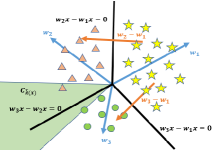
(a) $C_{q}$ (the green area).




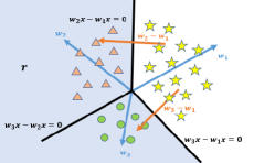
(b) $R_{q}$ (the blue area).



Figure 2: When $c=3$, $q=1$, the vectors $w_{q}$, $w_{l}$, $C_{q}$ and $R_{q}$.

 Then we will prove that $r$ can fool $c-1$ classes of data at the same time.
For a particular class $\hat{k}(x)=q$, we denote that polar cone of $C_{q}$ as $R_{q}^{c}=\{r\,|\,\langle r,v\rangle\leq 0,\ \forall\ v\in C_{q}\}$.
For $R_{q}^{c}$, since $w^{\top}_{q}r\geq w^{\top}_{l}r$, for all $l\in[c]$, $l\neq q$, we know that $R_{q}^{c}$
is the range where the data of class $q$ is located.
$R_{q}$ is the range where other $c-1$ classes data except class $q$ are located.
Suppose $r\in R_{\tilde{l}}^{c}$ for a fixed class $\tilde{l}$, so there is $\widetilde{P}_{T_{x}^{\tilde{l}}}\leq P_{T_{x}^{\tilde{l}}}\left(\left\{\max\limits_{l\in[c],\ l\neq{\tilde{l}}}(w_{l}^{\top}r-w^{\top}_{{\tilde{l}}}r)\right\}>0\right)=0$, i.e., the data of class ${\tilde{l}}$ cannot be fooled.
In this case, for all $q\in[c]$, $q\neq{\tilde{l}}$, we have $(w_{\tilde{l}}-w_{q})^{\top}r>0$,
and since $r$ is sufficiently large, then $\widetilde{P}_{T_{x}^{q}}>0$, $r\in R_{q}$. Further, we have $r\in R_{\tilde{l}}^{c}\subset\mathop{\cap}\limits_{q\in[c],\,q\neq{\tilde{l}}}R_{q}$. That is, except for the data of class $\tilde{l}$, other data can be fooled. Thus, we know that uAP of optimization problem Eq. 7 can fool $c-1$ class of data at most.
Since $r$ is sufficiently large, we get that all $\widetilde{P}_{T_{x}^{q}}$, $q\in[c]$ can reach the upper bound. Then to maximize Eq. 16, we select the label 




$$l^{*}_{u}=\mathop{\arg\min}\{\theta_{l}\,|\,l\in[c]\},$$


 such that $\widetilde{P}_{T_{x}^{l^{*}_{u}}}=0$ and $\widetilde{P}_{T_{x}^{q}}>0$, $q\in[c]$, $q\neq{l^{*}_{u}}$, i.e., $r\in R_{{l^{*}_{u}}}^{c}$, where $R_{{l^{*}_{u}}}^{c}$ is the distribution range of data with class $l^{*}_{u}$. The upper bound of $G_{\Omega,\hat{k}}$ on the linear multi-classifier can reach $1-\theta_{l^{*}_{u}}$. Approximately, we choose the vector $\dfrac{w_{{l^{*}_{u}}}}{\|w_{{l^{*}_{u}}}\|_{2}}$ that must belong to $R_{{l^{*}_{u}}}^{c}$ as the direction of uAP.
Under the constraint Eq. 7b, uAP of the linear multi-classifier on $\Omega$ is given by Eq. 15. 
Through Theorem 3.6 and Theorem 4.6, we realize that for SVM models, the data after adding uAP always falls into the region of a specific class (determined by the separating hyperplane), so uAP can not deceive all classes of data.



5 Numerical Experiments


In this section, we conduct extensive numerical test to verify the efficiency of our method. First, we introduce the datasets used in the experiment. The rest of the content is divided into two parts, and experiments are carried out on the adversarial perturbations in binary and multiclass linear SVMs.
All experiments are tested in Matlab R2019b in Windows 10 on a HP probook440 G2 with an Intel(R) Core(TM) i5-5200U CPU at 2.20 GHz and of 8 GB RAM.
All classifiers are trained using the LIBSVM [3] and LIBLINEAR [9] implementation, which can be downloaded from https://www.csie.ntu.edu.tw/$\sim$cjlin/libsvm and https://www.csie.ntu.edu.tw/$\sim$cjlin/liblinear. Other recent progress in SVM can be found in [11, 31, 32].


We test adversarial perturbations against SVMs on MNIST [19] and CIFAR-10 [15] image classification datasets. MNIST and CIFAR-10 are currently the most commonly used datasets, their settings are as follows:

• 

MNIST: The complete MNIST dataset has a total of 60,000 training samples and 10,000 test samples, each of which is a vector of 784 pixel values and can be restored to a $28*28$ pixel gray-scale handwritten digital picture. The value of the recovered handwritten digital picture ranges from 0 to 9, which exactly corresponds to the 10 labels of the dataset.

• 

CIFAR-10: CIFAR-10 is a color image dataset closer to universal objects. The complete CIFAR-10 dataset has a total of 50,000 training samples an 10,000 test samples, each of which is a vector of 3072 pixel values and can be restored to a $32*32*3$ pixel RGB color picture. There are 10 categories of pictures, each with 6000 images. The picture categories are airplane, automobile, bird, cat, deer, dog, frog, horse, ship and truck, their labels correspond to $\{0,1,2,3,4,5,6,7,8,9\}$ respectively.






5.1 Numerical experiments of binary linear SVMs


We present our experiments on the MNIST dataset and CIFAR-10 dataset on binary linear classification model. For MNIST, we extract the data with class 0 and 1 to form a new binary dataset, with a total of 12,665 training data and 2,115 test data. For CIFAR-10, due to the limitation of the computational complexity of training model, we only select a part of data with class dog and truck to form a new binary dataset, with a total of 3,891 training data and 803 test data.
First, we use LIBSVM to build a binary linear SVM on the training set, and obtain the parameters $w$ and $b$ of the classifier.
Then we use formulas Eq. 8, Eq. 10 and Eq. 11 to generate sAP, cuAP and uAP respectively.
Finally, we calculate $G_{\Omega,\hat{k}}$ of the uAP.



5.1.1 Numerical experiments of sAP


In Fig. 3, we give an example to compare the original image, the image that has been misclassified after being attacked, and the image of sAP on the MNIST dataset and CIFAR-10 dataset. By selecting the average of 10 repeated experiments on the same MNIST dataset, we get that the CPU time to train the binary classifier model is $1.37s$, and the average CPU time to generate sAP is only $5.33\times 10^{-4}s$. Similarly, on the CIFAR-10 dataset, we get the above CPU time as $53.49s$ and $3.04\times 10^{-2}s$ respectively.





(a) On the MNIST dataset, the original image class is 0 and the perturbed image class is 1.




(b) On the MNIST dataset, the original image class is 1 and the perturbed image class is 0.





(c) On the CIFAR-10 dataset, the original image class is dog and the perturbed image class is truck.




(d) On the CIFAR-10 dataset, the original image class is truck and the perturbed image class is dog.



Figure 3: The original image, the image that has been misclassified after being attacked, and the image of sAP on the MNIST and CIFAR-10 dataset.

 In Fig. 3a and Fig. 3b, we show the effect of adding sAP to handwritten digital images with original classes of 0 and 1, respectively. We obtain that the average norm of the data in the MNIST dataset is 8.79, the average norm of sAP is 1.74, and the signal to noise ratio (SNR) is 14.39. Although in human eyes, the classes of perturbed images do not change, but under the decision of the classifier, the classes of new images become 1 and 0 respectively.
For linear binary SVM, the directions of sAP of different classes of images are opposite, which can be reflected by the gray scale of sAP images in Fig. 3a and Fig. 3b.
In Fig. 3c and Fig. 3d, we show the effect of adding sAP to the images in CIFAR-10 dataset with original classes of dog and truck, respectively. The classes of perturbed images become truck and dog.
We obtain that the average norm of the data in the CIFAR-10 dataset is 30.45, the average norm of sAP is 0.13, and SNR is 50.03.
Comparing Fig. 3a and Fig. 3b on the MNIST dataset and Fig. 3c and Fig. 3d on the CIFAR-10 dataset, we find that on the binary classification model, the sAP generated on the dataset (CIFAR-10) with a larger number of features are less likely to be observed, and the human eye can hardly perceive the sAP image.



5.1.2 Numerical experiments of cuAP


In Fig. 4, we illustrate the effect of adding cuAP to the dataset when $\Omega$ is selected as the data with class 0 of MNIST dataset.
The class of all data in Fig. 4a is 0.
If they are attacked by the same cuAP shown in Fig. 4b, the perturbed new images will be displayed in the corresponding position in Fig. 4c, and the classifier will misclassify them as the number 1. In this case, the norm of cuAP is 2, and SNR is 12.57.
The CPU time for calculating the cuAP in Fig. 4b is only $1.06\times 10^{-4}s$. Because the process of generating cuAP does not need iteration.






(a) The original images with class 0.






(b) The image of the unique cuAP on the subset of MNIST dataset with class 0.






(c) The perturbed images with class 1.



Figure 4: The original images, the image of cuAP, and the images that have been misclassified after being attacked, when $\xi=2$ on the MNIST dataset.









(a) The original images with class truck.






(b) The image of the unique cuAP on the subset of CIFAR-10 dataset with class truck.






(c) The perturbed images with class dog.



Figure 5: The original images, the image of cuAP, and the images that have been misclassified after being attacked, when $\xi=0.5$ on the CIFAR-10 dataset.

Similarly, in Fig. 5, we give the original images with class truck, the image of cuAP and the perturbed images with class dog, when $\xi=0.5$ on the CIFAR-10 dataset. We get that the CPU time to generate cuAP is $7.25\times 10^{-3}s$ and SNR is 35.55.
Comparing Fig. 4 and Fig. 5, we find that cuAP generated on the dataset (CIFAR-10) with a larger number of features is less likely to be observed, and the perturbed images are almost the same as the original images by human observations.



5.1.3 Numerical experiments of uAP


Fig. 6 shows the relationship that the fooling rate with the size of uAP on the MNIST and CIFAR-10 real image data test set. Obviously, in Fig. 6a, we find that when the norm of uAP on the MNIST reaches 3, the fooling rate is almost $53.66\%$ and in Fig. 6b, when the norm of uAP on the CIFAR-10 reaches 0.5, the fooling rate is almost $52.93\%$. Comparing the results of different datasets on the same linear binary classifier in Fig. 6, we find that CIFAR-10 dataset is more likely to be fooled by very small uAP.





(a) The relationship on the MNIST dataset.




(b) The relationship on the CIFAR-10 dataset.



Figure 6: The relationship between the fooling rate and the norm of uAP obtained on the linear binary SVMs on the MNIST and CIFAR-10 dataset.







(a) The original images with class 1.






(b) The image of the unique uAP on the MNIST dataset.






(c) The perturbed images with class 0.



Figure 7: The original images, the image of uAP, and the images that have been misclassified after being attacked, when $\xi=2$ on the MNIST dataset.







(a) The original images with class dog.






(b) The image of the unique uAP on the CIFAR-10 dataset.






(c) The perturbed images with class truck.



Figure 8: The original images, the image of uAP, and the images that have been misclassified after being attacked, when $\xi=0.5$ on the CIFAR-10 dataset.


However, in reality, we should also consider that our uAP should not be observed by human beings, that is, the norm should be small enough. So we may not choose the uAP with the maximum fooling rate, but choose an appropriate size of uAP. In Fig. 7, we give an example to compare the original images, the image of uAP, and the images of that have been misclassified after being attacked, when $\xi=2$ on the MNIST dataset. In this case, SNR is 12.57. By selecting the average of 10 repeated experiments on the same MNIST test dataset, we get that the CPU time to generate uAP is only $2.05\times 10^{-5}s$. The process of generating uAP does not need iteration.
In Fig. 7a, the original images class are 1 and in Fig. 7c, the perturbed images class are 0. In MNIST dataset, because the proportion of data predicted as class 1 is larger, uAP mainly fools the data with class 1, as shown in Fig. 7b.
The image of uAP is small enough.


Similarly, in Fig. 8, we give the original images with class dog, the uAP and the perturbed image with class truck, when $\xi=0.5$ on the CIFAR-10 dataset. In this case, SNR is 35.55. In CIFAR-10 dataset, because the proportion of data predicted as class dog is larger, uAP mainly fools the data with class dog, as shown in Fig. 8b.
The CPU time to generate uAP is $5.65\times 10^{-4}s$.
Comparing Fig. 7 and Fig. 8, uAP generated on the dataset (CIFAR-10) with a larger number of features is less likely to be observed.







(a) 






(b) 







(c) 






(d) 







(e) 






(f) 







(g) 






(h) 







(i) 






(j) 



Figure 9: The original images with class $0,1,2,3,4,5,6,7,8,9$, the images that has been misclassified after being attacked with class $5,2,5,2,9,8,2,3,2,1$, and the images of sAP. 



5.2 Numerical experiments of multiclass linear SVMs


We present our experiments on the MNIST dataset and CIFAR-10 dataset on multiclass linear SVMs. For CIFAR-10, due to the limitation of the computational complexity of training model, we only select 5,000 training samples and 1,000 test samples from the original dataset.
First, we use LIBLINEAR to build a multiclass linear SVM on the training set, and obtain the parameters $w_{l}$, $l\in[c]$ of the classifier.
Then we use formulas Eq. 13, Eq. 14 and Eq. 15 to generate sAP, cuAP and uAP respectively.
Finally, we calculate $G_{\Omega,\hat{k}}$ of the uAP.



5.2.1 Numerical experiments of sAP


In Fig. 9, we give an example to compare the original image, the image that has been misclassified after being attacked, and the image of sAP on the MNIST dataset. By selecting the average of 10 repeated experiments on the same MNIST dataset, we get that the CPU time to train the multiclass classifier model is $35.78s$, and the average CPU time to generate sAP is only $3.12\times 10^{-3}s$.
The process of generating sAP does not need iteration.
In Fig. 9, the original images class are $0,1,2,3,4,5,6,7,8,9$. When we add sAP to the original images, the perturbed image class are $5,2,5,2,9,8,2,3,2,1$, but in human eyes, the class of the perturbed images have not changed. The average norm of the data in the MNIST dataset is 9.30, the average norm of sAP is 0.20, and SNR is 35.19.







(a) 






(b) 







(c) 






(d) 







(e) 






(f) 



Figure 10: The original images with class airplane, ship, bird, cat, deer and horse, the images that has been misclassified after being attacked with class ship, automobile, cat, horse, bird and deer, and the images of sAP. 


Similarly, on the CIFAR-10 dataset, we get that the CPU time to train the multiclass classifier model is $2.01\times 10^{3}s$, and the average CPU time to generate sAP is only $1.44\times 10^{-3}s$.
In Fig. 10, the original images class are airplane, ship, bird, cat, deer and horse. When we add the sAP to the original images, the perturbed image class are ship, automobile, cat, horse, bird and deer. It can be seen that animal images become another class of animal images after being attacked, and so are vehicle images.
This is because our generated sAP is based on the idea of attacking images to the most similar class, and our method generates the smallest sAP. We obtain that the average norm of the data in the CIFAR-10 dataset is 29.97, the average norm of sAP is 0.07, and SNR is 55.79.




5.2.2 Numerical experiments of cuAP


In Fig. 11,
we take numerical experiments on the MNIST dataset with class 6, and we get the CPU time to generate cuAP is only $5.11s$.
Fig. 11a show the original clean images with class 6.
If they are attacked by the same cuAP shown in Fig. 11b, the perturbed new images will be displayed in the corresponding position in Fig. 11c, and the classifier will misclassify them as the number 8. The norm of cuAP is 1, and SNR is 19.22.







(a) The original images with class 6.






(b) The image of the unique cuAP on the subset of MNIST dataset with class 6.






(c) The perturbed images with class 8.



Figure 11: The original images, the image of cuAP, and the images that have been misclassified after being attacked, when $\xi=1$ on the MNIST dataset.







(a) The original images with class horse.






(b) The image of the unique cuAP on the subset of CIFAR-10 dataset with class horse.






(c) The perturbed images with class deer.



Figure 12: The original images, the image of cuAP, and the images that have been misclassified after being attacked, when $\xi=0.5$ on the CIFAR-10 dataset.


Similarly, in Fig. 12, we give the original images with class horse, the image of cuAP and the perturbed images with class deer, when $\xi=0.5$ on the CIFAR-10 dataset. In this case, SNR is 35.35.
And we get that the CPU time to generate cuAP is $2.71s$.
Comparing Fig. 11 and Fig. 12, we find that cuAP generated on the dataset (CIFAR-10) with a larger number of features is more difficult to be observed.




5.2.3 Numerical experiments of uAP


Fig. 13 shows the relationship that the fooling rate increases with the increase of the size of uAP on the MNIST and CIFAR-10 datasets. In Fig. 13a, we find that when the norm of uAP on the MNIST reaches 1, the fooling rate is almost $90.48\%$ and in Fig. 13b, when the norm of uAP on the CIFAR-10 reaches 0.5, the fooling rate is almost $89.60\%$. We find that the dataset in Fig. 13b, which has more features, is easier to be fooled by very small perturbation.
However, with the increase of the norm of uAP, the fooling rate will not increase to $100\%$. In reality, we may choose an appropriate size of uAP, when the fooling rate is large enough.





(a) The relationship on the MNIST dataset.




(b) The relationship on the CIFAR-10 dataset.



Figure 13: The relationship between the fooling rate and the norm of uAP obtained on the linear multiclass SVMs on the MNIST and CIFAR-10 datasets.


In Fig. 14, we give an example to compare the original images, the image of uAP, and the images of that have been misclassified after being attacked, when $\xi=1$ on the MNIST dataset.
In this case, SNR is 19.22.
The CPU time to generate uAP is only $3.05\times 10^{-3}s$.
In MNIST dataset, because the proportion of data predicted as class 5 is the smallest, the direction of uAP points to class 5.


Figure 14: When added to a natural image, uAP causes the image to be misclassified by the linear multiclass SVMs on the MNIST dataset. Left images: Original images.
The classes are shown at each arrow. Central image: uAP. Right images: Perturbed images. The estimated classes of the perturbed images are shown at each arrow, which are 5.


In Fig. 15, the original images are bird, cat, deer, dog, frog, horse and ship on the CIFAR-10 dataset. When we add uAP ($\xi=0.5$) to the original images, the perturbed images are automobiles, but in human eyes, the class of the perturbed images have not changed. In this case, SNR is 35.35. The CPU time to generate uAP is only $8.86\times 10^{-4}s$.
Comparing Fig. 14 and Fig. 15, we find that on the multi-classification model, the data with the same distribution are easy to be attacked by the uAP with unique direction and size, and the perturbation generated on the dataset (CIFAR-10) with a larger number of features is less likely to be observed.


Figure 15: When added to a natural image, uAP causes the image to be misclassified by the linear multiclass SVMs on the CIFAR-10 dataset. Left images: Original images.
The classes are shown at each arrow. Central image: uAP. Right images: Perturbed images. The estimated classes of the perturbed images are shown at each arrow, which are automobiles.


Obviously, the multi-classification tasks are more likely to be fooled by smaller perturbation than binary classification tasks, because its classification boundary is closer. Therefore, we speculate that the reason for the existence of adversarial perturbations is that the flexibility of the classifier is lower than the difficulty of the classification task. As we all know, SVM, neural network and most machine learning models are discriminant models, whose purpose is to find the optimal separating hyperplane between different class.
Different from the generative model, it mainly focuses on the differences between different class of data, and cannot reflect the characteristics of the data itself, so it will produce some defects.



6 Conclusions


In this paper, we propose the optimization models for the adversarial perturbations on classification based on SVMs.
We derive the explicit solutions for sAP, cuAP and uAP (binary case), and approximate solution for uAP of multi-classification. We also provided the upper bound for the fooling rate of uAP.
Moreover, we increase the interpretability of adversarial perturbations which shows that the directions of adversarial perturbations are related to the separating hyperplanes of the model and the size is related to the fooling rate. Numerical results demonstrate that our proposed approach can generate efficient adversarial perturbations for models trained by SVMs. It is extremely fast for linear training models since one can avoid iteration process in this case. Numerical results also show some insights on the potential security vulnerabilities of machine learning models.

References

[1]A. Antikacioglu, T. Bajpai, and R. Ravi, A new system-wide diversity
measure for recommendations with efficient algorithms, SIAM Journal on
Mathematics of Data Science, 1 (2019), pp. 759–779,
https://doi.org/10.1137/18M1226014.
[2]P. Benz, C. Zhang, T. Imtiaz, and I. S. Kweon, Double targeted
universal adversarial perturbations, Proceedings of the Asian Conference on
Computer Vision, (2020), https://doi.org/10.1007/978-3-030-69538-5_18.
[3]C.-C. Chang and C.-J. Lin, LIBSVM: A library for support
vector machines, ACM Transactions on Intelligent Systems and Technology, 2
(2011), pp. 1–27, https://doi.org/10.1145/1961189.1961199.
[4]E. C. Chi and S. Steinerberger, Recovering trees with convex
clustering, SIAM Journal on Mathematics of Data Science, 1 (2019),
pp. 383–407, https://doi.org/10.1137/18M121099X.
[6]K. Crammer and Y. Singer, On the algorithmic implementation of
multiclass kernel-based vector machines, Journal of Machine Learning
Research, 2 (2001), pp. 265–292.
[7]M. Crawford, T. M. Khoshgoftaar, J. D. Prusa, A. N. Richter, and H. A.
Najada, Survey of review spam detection using machine learning
techniques, Journal of Big Data, 2 (2015), pp. 1–24,
https://doi.org/10.1186/s40537-015-0029-9.
[8]C. Cui, K. Zhang, T. Daulbaev, J. Gusak, I. Oseledets, and Z. Zhang, Active subspace of neural networks: Structural analysis and universal
attacks, SIAM Journal on Mathematics of Data Science, 2 (2020),
pp. 1096–1122, https://doi.org/10.1137/19M1296070.
[9]R.-E. Fan, K.-W. Chang, C.-J. Hsieh, X.-R. Wang, and C.-J. Lin, LIBLINEAR: A library for large linear classification, the Journal
of Machine Learning Research, 9 (2008), pp. 1871–1874,
https://doi.org/10.1145/1390681.1442794.
[10]A. Fawzi, O. Fawzi, and P. Frossard, Analysis of classifiers’
robustness to adversarial perturbations, Machine Learning, 107 (2018),
pp. 481–508, https://doi.org/10.1007/s10994-017-5663-3.
[11]L. Galli and C.-J. Lin, A study on truncated newton methods for
linear classification, IEEE Transactions on Neural Networks and Learning
Systems, (2021), pp. 1–14,
https://doi.org/10.1109/TNNLS.2020.3045836.
[12]I. J. Goodfellow, J. Shlens, and C. Szegedy, Explaining and
harnessing adversarial examples, (2014),
https://arxiv.org/abs/1412.6572.
[13]A. Graves, S. Fernández, F. Gomez, and J. Schmidhuber, Connectionist temporal classification: Labelling unsegmented sequence data
with recurrent neural networks, Proceedings of the 23rd international
conference on Machine learning, (2006), pp. 369–376,
https://doi.org/10.1145/1143844.1143891.
[14]L. Huang, A. D. Joseph, B. Nelson, B. I. Rubinstein, and J. D. Tygar,
Adversarial machine learning, Proceedings of the 4th ACM Workshop on
Security and Artificial Intelligence, (2011), pp. 43–58,
https://doi.org/10.1145/2046684.2046692.
[15]A. Krizhevsky, Learning Multiple Layers of Features from Tiny
Images, University of Toronto, Toronto, 2009.
[16]A. Krizhevsky, I. Sutskever, and G. E. Hinton, Imagenet
classification with deep convolutional neural networks, Advances in Neural
Information Processing Systems, 25 (2012), pp. 1097–1105,
https://doi.org/10.1145/3065386.
[18]P. Langenberg, E. Balda, A. Behboodi, and R. Mathar, On the
robustness of support vector machines against adversarial examples, 2019
13th International Conference on Signal Processing and Communication Systems,
(2019), pp. 1–6, https://doi.org/10.1109/ICSPCS47537.2019.9008746.
[19]Y. Lecun, L. Bottou, Y. Bengio, and P. Haffner, Gradient-based
learning applied to document recognition, Proceedings of the IEEE, 86
(1998), pp. 2278–2324, https://doi.org/10.1109/5.726791.
[20]T. Miyato, S.-I. Maeda, M. Koyama, and S. Ishii, Virtual adversarial
training: A regularization method for supervised and semi-supervised
learning, IEEE Transactions on Pattern Analysis and Machine Intelligence, 41
(2018), pp. 1979–1993, https://doi.org/10.1109/TPAMI.2018.2858821.
[21]S.-M. Moosavi-Dezfooli, A. Fawzi, O. Fawzi, and P. Frossard, Universal adversarial perturbations, Proceedings of the IEEE Conference on
Computer Vision and Pattern Recognition, (2017), pp. 1765–1773,
https://doi.org/10.1109/CVPR.2017.17.
[22]S.-M. Moosavi-Dezfooli, A. Fawzi, and P. Frossard, Deepfool: A
simple and accurate method to fool deep neural networks, Proceedings of the
IEEE Conference on Computer Vision and Pattern Recognition, (2016),
pp. 2574–2582, https://doi.org/10.1109/CVPR.2016.282.
[23]K. R. Mopuri, U. Garg, and R. V. Babu, Fast feature fool: A data
independent approach to universal adversarial perturbations, (2017),
https://arxiv.org/abs/1707.05572.
[24]K. R. Mopuri, U. Ojha, U. Garg, and R. V. Babu, Nag: Network for
adversary generation, Proceedings of the IEEE Conference on Computer Vision
and Pattern Recognition, (2018), pp. 742–751,
https://doi.org/10.1109/CVPR.2018.00084.
[25]F. Ricci, L. Rokach, and B. Shapira, Introduction to recommender
systems handbook, Recommender Systems Handbook, (2011), pp. 1–35,
https://doi.org/10.1007/978-0-387-85820-3_1.
[26]T. Schnabel, P. N. Bennett, S. T. Dumais, and T. Joachims, Using
shortlists to support decision making and improve recommender system
performance, Proceedings of the 25th International Conference on World Wide
Web, (2016), pp. 987–997, https://doi.org/10.1145/2872427.2883012.
[27]J. Suykens and J. Vandewalle, Least squares support vector machine
classifiers, Neural Processing Letters, 9 (1999), pp. 293–300,
https://doi.org/10.1023/A:1018628609742.
[28]C. Szegedy, W. Zaremba, I. Sutskever, J. Bruna, D. Erhan, I. Goodfellow,
and R. Fergus, Intriguing properties of neural networks, (2013),
https://arxiv.org/abs/1312.6199.
[29]N. Veldt, D. F. Gleich, A. Wirth, and J. Saunderson, Metric-constrained optimization for graph clustering algorithms, SIAM
Journal on Mathematics of Data Science, 1 (2019), pp. 333–355,
https://doi.org/10.1137/18M1217152.
[30]B. Wang, B. Yuan, Z. Shi, and S. J. Osher, Enresnet: Resnets
ensemble via the feynman–kac formalism for adversarial defense and beyond,
SIAM Journal on Mathematics of Data Science, 2 (2020), pp. 559–582,
https://doi.org/10.1137/19M1265302.
[31]Y. Yan and Q. Li, An efficient augmented lagrangian method for
support vector machine, Optimization Methods and Software, 35 (2020),
pp. 855–883, https://doi.org/10.1080/10556788.2020.1734002.
[32]J. Yin and Q. Li, A semismooth newton method for support vector
classification and regression, Computational Optimization and Applications,
73 (2019), pp. 477–508, https://doi.org/10.1007/s10589-019-00075-z.
[33]T. Young, D. Hazarika, S. Poria, and E. Cambri, Recent trends in
deep learning based natural language processing, IEEE Computational
Intelligence Magazine, 13 (2018), pp. 55–75,
https://doi.org/10.1109/MCI.2018.2840738.
[34]C. Zhang, P. Benz, T. Imtiaz, and I.-S. Kweon, CD-UAP:
Class discriminative universal adversarial perturbation, Proceedings of the
AAAI Conference on Artificial Intelligence, 34 (2020), pp. 6754–6761,
https://doi.org/10.1609/aaai.v34i04.6154.
[35]Y. Zhou, M. Kantarcioglu, B. Thuraisingham, and B. Xi, Adversarial
support vector machine learning, Proceedings of the 18th ACM SIGKDD
International Conference on Knowledge Discovery and Data Mining, (2012),
pp. 1059–1067, https://doi.org/10.1145/2339530.2339697.