Non-commutativity and non-inertial effects on a scalar field in a cosmic string space-time
Part 2: Spin-zero Duffin-Kemmer-Petiau-like oscillator

Rodrigo Rocha Cuzinatto^a, Marc de Montigny^b, Pedro José Pompeia^{c a}Instituto de Ciência e Tecnologia, Universidade Federal de Alfenas
Rodovia José Aurélio Vilela, 11999, Cidade Universitária
CEP 37715-400 Poços de Caldas, Minas Gerais, Brazil ^bFaculté Saint-Jean, University of Alberta
8406 91 Street NW
Edmonton, Alberta, Canada T6C 4G9, Canada ^cDepartamento de Física, Instituto Tecnológico de Aeronáutica
Praça Mal. Eduardo Gomes 50
CEP 12228-900 São José dos Campos, São Paulo, Brazil

We study the non-inertial effects of a rotating frame on a spin-zero, Duffin-Kemmer-Petiau (DKP)-like oscillator in a cosmic string space-time with non-commutative geometry in the momentum space. The spin-zero DKP-like oscillator is obtained from the Klein-Gordon Lagrangian with a non-standard prescription for the oscillator coupling. We find that the solutions of the time-independent radial equation with the non-zero non-commutativity parameter parallel to the string are related to the confluent hypergeometric function. We find the quantized energy eigenvalues of the non-commutative oscillator.

Keywords: Spin-zero oscillator, cosmic string, rotating frame, non-commutative geometry.

1 Introduction

A common approach to the theory of spin-zero fields involves second-order differential equations of motion, such as the Klein-Gordon (KG) equation (e.g. see Ref. [1]). The Duffin-Kemmer-Petiau (DKP) equation [2, 3, 4, 5] was an attempt to obtain first-order field equations for fields with integer spin analogous to the Dirac equation for spin-half fields. Both descriptions are not always equivalent and, for this reason, it is key to characterize the phenomenology associated both to KG field and DKP field so that experimental results can ultimately decide in favour of one description over the other [6, 7].

Even though the equivalence between the DKP and KG equations for interacting spin-zero fields is not absolute [8], at least, it is well known that both are equivalent for free fields. For interacting fields, a coupling prescription is required and it can be introduced either by symmetry or by phenomenological arguments. We should keep in mind that different prescriptions lead to different results, and each case should be analyzed separately [9]. The DKP equation lends itself to a richness of couplings that are not all equivalent to KG theories [10, 11]. The fundamental point in this regard is to address whether it is possible to obtain a second-order differential equation for a spin-zero field that leads to an equivalent DKP-oscillator equation. In this paper, we will consider a system for which it is indeed possible to obtain such equation. However, there will be a price to pay: the oscillator coupling has to be different from the ordinary prescription. Indeed, as we did in Ref. [12], the standard oscillator prescription consists of taking the non-minimal coupling

$$\begin{split}&\mathbf{p}\phi\rightarrow\ \left(\mathbf{p}-im\omega_{0}\mathbf{r}\right)\phi,\\ &\mathbf{p}\phi^{*}\rightarrow\ \left(\mathbf{p}+im\omega_{0}\mathbf{r}\right)\phi^{*},\end{split}$$ (1)

where $m$ is the mass of the complex scalar field $\phi$ localized by coordinate $\mathbf{r}$ and momentum $\boldsymbol{{\rm p}}$, and $\omega_{0}$ is the oscillator’s frequency. This leads to the so-called ‘KG-oscillator’.

Hereafter, we shall take a different path and consider a similar prescription but without modifying the sign of the operator $\mathbf{r}$, as we did in Eq. (1) for the field and its conjugate. We will see that that second path leads to a second-order equation which is equivalent to the DKP-oscillator. We intend to explore the role of this alternative prescription upon the behavior of a spin-zero field oscillator. Physically, different couplings may lead to distinct effects through the interaction. Our goal is to compare the results herein with those obtained in Ref. [12], hence referred to as Part 1.

In Part 1, besides considering the oscillator prescription, we also took into account the effects of non-commutativity in momentum space via

$$\begin{split}&\mathbf{p}\phi\rightarrow\ \left(\mathbf{p}-\frac{\boldsymbol{\Omega}\times\mathbf{r}}{2}\right)\phi,\\ &\mathbf{p}\phi^{*}\rightarrow\ \left(\mathbf{p}+\frac{\boldsymbol{\Omega}\times\mathbf{r}}{2}\right)\phi^{*},\end{split}$$ (2)

where $\boldsymbol{\Omega}$ is the non-commutative vector parameter. The sign choices in Eqs.(1) and (2) are clearly similar. Analogously, in this work we will demand consistency between the choice of sign in the DKP-like oscillator prescription and the choice of sign in the recipe for introducing non-commutativity.

We will analyze the spin-zero DKP-like oscillator in a cosmic string spacetime, which, in a rotating frame, is described by the line element

$$ds^{2}=-\left(1-\omega^{2}\eta^{2}\rho^{2}\right)dt^{2}+2\omega\eta^{2}\rho^{2}d\varphi dt+d\rho^{2}+\eta^{2}\rho^{2}d\varphi^{2}+dz^{2}.$$ (3)

We use cylindrical coordinates $(\rho,\varphi,z)$, where $\rho\in[0,\infty),\,\varphi\in[0,2\pi],\,z\in(-\infty,+\infty)$, and natural units where $c=\hbar=1$. The angular frequency of the rotating frame is given by $\omega$; the string parameter is $\eta=1-4\Lambda\in(0,1]$, where $\Lambda$ is the topological defect linear mass density (see Refs. [18, 19, 20, 21] for other applications). Notice that this line element is singular at the hard-wall

$$\rho_{0}\equiv\frac{1}{\omega\eta}.$$ (4)

As a consequence, our particle should be confined within $0\leqslant\rho<\rho_{0}$, which means that the wave function has to vanish at the hard-wall. Hereafter, we shall consider a similar situation as in Part 1, where we examined a KG-oscillator in the presence of non-commutativity in a rotating frame in a cosmic string spacetime [12]. Therein, we observed that non-commutativity was responsible for changing the energy eigenstates of the particle both when the hard-wall is at a finite position and when the hard-wall’s position approaches infinity. There, we saw that we can interpret the non-commutativity parameter as a constant magnetic field pointing in the direction of the string. Hereafter, a similar interpretation does not hold due to a difference of sign in the coupling, cf. Section 2. Even without that connection between non-commutativity and a magnetic field, in this paper, we are able to describe a spin-zero DKP-like oscillator. More details about the DKP oscillator can be found in Refs. [22, 23, 24] and references therein. Moreover, we can shed light on how the coupling between the field and non-commutativity could be carried out. Recall that in the case of the electromagnetic interaction, the coupling between the scalar field and the electromagnetic potential is determined by the minimal coupling prescription, which is a consequence of the underlying $U\left(1\right)$ gauge symmetry. With non-commutativity, this coupling is not connected with any gauge symmetry and could be introduced in at least two different ways: one is presented in Eq. (2) and was explored in Part 1, in which the focus was on the mapping between non-commutativity and a magnetic field; the other is to apply $\mathbf{p}\rightarrow\ \mathbf{p}-\frac{\boldsymbol{\Omega}\times\mathbf{r}}{2}$ to both $\phi$ and $\phi^{*}$. The latter possibility is the one explored here and we focus on the effects of the different choice of coupling prescription for the non-commutativity upon the physical system.

In Section 2, we define the KG Lagrangian and establish the field equation for the spin-zero DKP-like oscillator in a non-inertial frame and cosmic string space-time with non-commutative geometry. We thus obtain an equation in terms of time and cylindrical coordinates, which we solve in Section 2.1 with the only non-zero non-commutativity parameter parallel to the cosmic string. The solution along that axis is in terms of the Hermite polynomials, whereas the radial solutions are expressed in terms of the confluent hypergeometric functions. We discuss the corresponding energy eigenvalues in Section 3: with the hard-wall at infinity in Section 3.1 and at a finite distance from the cosmic string in Section 3.2. We complete the paper with concluding remarks in Section 4.

2 Spin-zero DKP-like oscillator in a non-inertial frame and cosmic string space-time with non-commutative geometry

The equation for the DKP-like oscillator is obtained from the KG equation with the non-minimal coupling [13, 14, 15, 16]:

$$\mathbf{p}\rightarrow\ \mathbf{p}-im\omega_{0}\mathbf{r},$$ (5)

where we use cylindrical coordinates and select

$$\mathbf{r}=\rho\hat{e}_{\rho}+z\hat{e}_{z}=\left(\rho,0,z\right).$$ (6)

Since $p_{j}=-{\rm i}\partial_{j}$ ($j=1,2,3$), Eq. (5) is $-{\rm i}\left(\nabla\pm m\omega_{0}\mathbf{r}\right)$.

If we begin with the KG Lagrangian

$$L=\sqrt{-g}\left(-g^{ab}\partial_{a}\phi^{*}\partial_{b}\phi-m^{2}\phi^{*}\phi\right),$$ (7)

and perform the non-minimal substitution of Eq. (5), we obtain the Lagrangian of the KG oscillator:

$$L_{\mathrm{osc}} = -\sqrt{-g}\left[g^{00}\partial_{0}\phi^{*}\partial_{0}\phi+g^{02}\partial_{0}\phi^{*}\partial_{2}\phi+g^{02}\partial_{2}\phi^{*}\partial_{0}\phi\right.$$

$$+g^{11}\left(\partial_{1}\phi^{*}+m\omega_{0}\rho\phi^{*}\right)\left(\partial_{1}\phi+m\omega_{0}\rho\phi\right)+g^{22}\partial_{2}\phi^{*}\partial_{2}\phi$$

$$\left.+g^{33}\left(\partial_{3}\phi^{*}+m\omega_{0}z\phi^{*}\right)\left(\partial_{3}\phi+m\omega_{0}z\phi\right)+m^{2}\phi^{*}\phi\right],$$

which, with 0, 1, 2, 3 standing for $t$, $\rho$, $\varphi$ and $z$, respectively, leads to the equation of motion

$$-m^{2}\phi-m^{2}\omega_{0}^{2}\rho^{2}\phi-m^{2}\omega_{0}^{2}z^{2}\phi-\partial_{0}^{2}\phi+\frac{1}{\rho}\partial_{1}\phi+\partial_{1}^{2}\phi+\left(\frac{1}{\eta^{2}\rho^{2}}-\omega^{2}\right)\partial_{2}^{2}\phi+2\omega\partial_{2}\partial_{0}\phi+\partial_{3}^{2}\phi+3m\omega_{0}\phi=0.$$ (9)

Next we introduce the non-commutative momentum space. Consider a non-commutative phase space described by the operators $\hat{r}_{i}$ and $\hat{p}_{i}$,

$$\hat{r}_{i} =r_{i}-\frac{\Theta_{ij}}{2\hbar}p_{j}=r_{i}+\frac{\left(\mathbf{\Theta}\times{\bf p}\right)_{i}}{2\hbar},$$ (10)

$$\hat{p}_{i} =p_{i}+\frac{\Omega_{ij}}{2\hbar}r_{j}=p_{i}-\frac{\left(\mathbf{\Omega}\times{\bf r}\right)_{i}}{2\hbar},$$ (11)

which satisfy the following commutation relations:

$$\left[\hat{r}_{i},\hat{r}_{j}\right]={\rm i}\Theta_{ij},\quad\left[\hat{p}_{i},\hat{p}_{j}\right]={\rm i}\Omega_{ij},\quad\left[\hat{r}_{i},\hat{p}_{j}\right]={\rm i}\hbar\Delta_{ij},$$ (12)

where $\Theta_{ij}=\epsilon_{ijk}\Theta_{k}$, $\Omega_{ij}=\epsilon_{ijk}\Omega_{k}$, with $\Theta_{i}$ and $\Omega_{i}$ ($i=1,2,3$) real parameters. The matrix $\Delta_{ij}$ is given by

$$\Delta_{ij}=\left(1+\frac{\mathbf{\Theta}\cdot\mathbf{\Omega}}{4\hbar^{2}}\right)\delta_{ij}-\frac{\Omega_{i}\Theta_{j}}{4\hbar^{2}}.$$ (13)

From the onset, we will restrict our study to

$$\Theta_{j}=0,\quad j=1,2,3,$$ (14)

so that we allow for a non-commutative momentum space only, whereas the configuration space for the cosmic string remains commutative for reasons discussed in Paper 1. Therefore, the non-commutative phase-space components are

$$\hat{r}_{i}=r_{i},$$

$$\hat{p}_{i}=p_{i}+\frac{\Omega_{ij}}{2}r_{j}=p_{i}-\frac{\left(\mathbf{\Omega}\times{\bf r}\right)_{i}}{2},$$ (15)

so that the commutation relations read

$$\left[\hat{r}_{i},\hat{r}_{j}\right]=0,\quad\left[\hat{p}_{i},\hat{p}_{j}\right]={\rm i}\Omega_{ij},\quad\left[\hat{r}_{i},\hat{p}_{j}\right]={\rm i}\hbar\delta_{ij}.$$ (16)

In cylindrical coordinates, the second term of Eq. (15) is

$$\frac{\Omega_{ij}}{2}r_{j}=\frac{1}{2}\left(\Omega_{13}z,\Omega_{21}\rho+\Omega_{23}z,\Omega_{31}\rho\right)=\frac{1}{2}\left(-\Omega_{2}z,-\Omega_{3}\rho+\Omega_{1}z,\Omega_{2}\rho\right).$$ (17)

Then, Eq. (2) is generalized to the non-commutative oscillator Lagrangian:

$$L_{\mathrm{NC-osc}} = -\sqrt{-g}\left[g^{00}\partial_{0}\phi^{*}\partial_{0}\phi+g^{02}\partial_{0}\phi^{*}\left(\partial_{2}\phi+i\frac{1}{2}\Omega_{3}\rho\phi-\frac{1}{2}i\Omega_{1}z\phi\right)\right.$$ (18)

$$+g^{02}\left(\partial_{2}\phi^{*}+\frac{1}{2}i\Omega_{3}\rho\phi^{*}-\frac{1}{2}i\Omega_{1}z\phi^{*}\right)\partial_{0}\phi$$

$$+g^{11}\left(\partial_{1}\phi^{*}+m\omega_{0}\rho\phi^{*}+\frac{1}{2}i\Omega_{2}z\phi^{*}\right)\left(\partial_{1}\phi+m\omega_{0}\rho\phi+\frac{1}{2}i\Omega_{2}z\phi\right)$$

$$+g^{22}\left(\partial_{2}\phi^{*}+\frac{1}{2}i\Omega_{3}\rho\phi^{*}-\frac{1}{2}i\Omega_{1}z\phi^{*}\right)\left(\partial_{2}\phi+i\frac{1}{2}\Omega_{3}\rho\phi-\frac{1}{2}i\Omega_{1}z\phi\right)$$

$$\left.+g^{33}\left(\partial_{3}\phi^{*}+m\omega_{0}z\phi^{*}-\frac{1}{2}i\Omega_{2}\rho\phi^{*}\right)\left(\partial_{3}\phi+m\omega_{0}z\phi-\frac{1}{2}i\Omega_{2}\rho\phi\right)+m^{2}\phi^{*}\phi\right],$$

which modifies Eq. (9) as follows:

$$\begin{array}[]{ccc}-m^{2}\phi+3m\omega_{0}\phi-\left(m\omega_{0}\rho+i\frac{1}{2}\Omega_{2}z\right)^{2}\phi-\left(m\omega_{0}z-i\frac{1}{2}\Omega_{2}\rho\right)^{2}\phi\\ -\left(\frac{1}{\eta^{2}\rho^{2}}-\omega^{2}\right)\left(i\frac{1}{2}\Omega_{3}\rho-i\frac{1}{2}\Omega_{1}z\right)^{2}\phi+i\frac{1}{2}\Omega_{2}\frac{z}{\rho}\phi\\ +\frac{1}{\rho}\partial_{1}\phi+2\omega\partial_{0}\partial_{2}\phi-\partial_{0}^{2}\phi+\partial_{1}^{2}\phi+\left(\frac{1}{\eta^{2}\rho^{2}}-\omega^{2}\right)\partial_{2}^{2}\phi+\partial_{3}^{2}\phi=0.\end{array}$$ (19)

In the next section, we will further simplify our problem with $\Omega_{3}$ being the only non-zero non-commutativity parameter.

2.1 Solution to the (momentum-space) non-commutative field equation

Now we look for the corresponding time-independent solution $\psi(\rho,\varphi,z)$ of Eq. (19), defined by

$$\phi\left(\rho,\varphi,z,t\right)=e^{-i{\cal E}t}\psi\left(\rho,\varphi,z\right),$$ (20)

where ${\cal E}$ is the energy, so that Eq. (19) is reduced to

$$-m^{2}\psi+3m\omega_{0}\psi+\left(\frac{1}{4}\Omega_{2}^{2}-m^{2}\omega_{0}^{2}\right)\left(\rho^{2}+z^{2}\right)\psi+\left(\frac{1}{\eta^{2}\rho^{2}}-\omega^{2}\right)\left(\frac{1}{2}\Omega_{3}\rho-\frac{1}{2}\Omega_{1}z\right)^{2}\psi$$

$$+\frac{1}{2}i\Omega_{2}\frac{z}{\rho}\psi+\frac{1}{\rho}\partial_{\rho}\psi-2i\omega\mathcal{E}\partial_{\varphi}\psi+{\cal E}^{2}\psi+\partial_{\rho}^{2}\psi+\left(\frac{1}{\eta^{2}\rho^{2}}-\omega^{2}\right)\partial_{\varphi}^{2}\psi+\partial_{z}^{2}\psi=0.$$ (21)

We note that the non-commutativity parameters ${\bf{\Omega}}$ only couple to the frame angular velocity $\omega$ of Eq. (3), so that there is no coupling with the oscillator frequency $\omega_{0}$ of Eq. (5). Moreover, we observe that the hard-wall condition is manifest through the factors $\frac{1}{\eta^{2}\rho^{2}}-\omega^{2}$ in Eq. (21), as it was in Eqs. (9) and (19).

At this point, if, in order to find a solution, we use the method of separation of variables, we can observe from Eq. (21) that this method is not easily applicable, since there are terms that involves the product of coordinates $\rho$ and $z$: $\frac{1}{2}i\Omega_{2}\frac{z}{\rho}\psi$ and $\left(\frac{1}{\eta^{2}\rho^{2}}-\omega^{2}\right)\left(\frac{1}{2}\Omega_{3}\rho-\frac{1}{2}\Omega_{1}z\right)^{2}\psi$. We avoid this problem by selecting the particular case,

$$\Omega_{1}=\Omega_{2}=0,$$ (22)

so that we take $\Omega_{3}\neq 0$ only. This particular choice is not only convenient from the computational stand point, but also physically meaningful as shown in the discussion above on the mapping of momentum-space non-commutativity with $\Omega_{3}\neq 0$ to a constant magnetic field pointing in the $z$-direction [17]. We implement the separation of variables:

$$\psi\left(\rho,\varphi,z\right)=R\left(\rho\right)\Phi\left(\varphi\right)Z\left(z\right),$$ (23)

which we substitute in Eq. (21) and obtain

$${\cal E}^{2}-m^{2}+3m\omega_{0}+\left[\left(\frac{1}{\eta^{2}\rho^{2}}-\omega^{2}\right)\frac{1}{4}\Omega_{3}^{2}-m^{2}\omega_{0}^{2}\right]\rho^{2}+\frac{1}{\rho}\frac{1}{R\left(\rho\right)}\partial_{\rho}R\left(\rho\right)+\frac{1}{R\left(\rho\right)}\partial_{\rho}^{2}R\left(\rho\right)$$

$$-m^{2}\omega_{0}^{2}z^{2}+\frac{1}{Z\left(z\right)}\partial_{z}^{2}Z\left(z\right)-2i\omega\mathcal{E}\frac{1}{\Phi\left(\varphi\right)}\partial_{\varphi}\Phi\left(\varphi\right)+\left(\frac{1}{\eta^{2}\rho^{2}}-\omega^{2}\right)\frac{1}{\Phi\left(\varphi\right)}\partial_{\varphi}^{2}\Phi\left(\varphi\right)=0.$$ (24)

In order to further decouple this equation, we utilize the azimuthal coordinate ansatz:

$$\Phi=e^{iL\varphi},$$ (25)

which is subject to the familiar boundary condition $\Phi\left(2\pi\right)=\Phi\left(0\right)$, so that $e^{iL\left(2\pi\right)}=1$, which leads to the quantization of the number $L$ in Eq. (25):

$$L=0,\pm 1,\pm 2,\pm 3,\cdots$$ (26)

Let us set the $z$-dependent part equal to a constant,

$$\frac{1}{Z}\left[\partial_{z}^{2}Z-\left(m\omega_{0}\right)^{2}z^{2}Z\right]=-2mk,$$ (27)

where $m$ is the mass of the Klein-Gordon field, and $k$ a new constant with units of energy. We replace the variable $z$ with the dimensionless variable $\zeta$,

$$\zeta\equiv\sqrt{m\omega_{0}}z.$$ (28)

Then Eq. (27) is simplified to

$$\frac{d^{2}Z}{d\zeta^{2}}=\left[\zeta^{2}-\frac{2k}{\omega_{0}}\right]Z=\left[\zeta^{2}-K\right]Z,$$ (29)

where

$$K\equiv\frac{2k}{\omega_{0}}.$$ (30)

This occurrence of an energy unit of the quantum harmonic oscillator manifests the oscillatory nature of the model. This is also shown by the fact that Eq. (29) is exactly the harmonic oscillator differential equation (see, e.g. Ref. [25]). Thus the solutions for $Z(\zeta)$ are given in terms of Hermite polynomials:

$$Z\left(\zeta\right)=\left(\frac{m\omega_{0}}{\pi}\right)^{1/4}\frac{1}{\sqrt{2^{m_{z}}m_{z}!}}H_{m_{z}}\left(\zeta\right)e^{-\zeta^{2}/2},$$ (31)

where $m_{z}=0,1,2,\cdots$ Note also that the recursion formula of the Frobenius expansion requires $K=2m_{z}+1$, which, from Eq. (30), leads to the quantization of $k$

$$k=\omega_{0}\left(m_{z}+\frac{1}{2}\right)\,,\qquad m_{z}=0,1,2,...$$ (32)

Although the normalization factor in Eq. (31) is not particularly relevant at this point, we choose it such that the coefficient of the highest power in $\zeta$ is $2^{m_{z}}$, as in Ref. [26].

Finally, let us turn to the most intricate part of Eq. (24): the radial part, which reads

$$\frac{d^{2}R}{d\rho^{2}}+\frac{1}{\rho}\frac{dR}{d\rho}-\left[\left(m\omega_{0}\right)^{2}+\left(\frac{\Omega_{3}}{2}\omega\right)^{2}\right]\rho^{2}R-\left(\frac{L}{\eta}\right)^{2}\frac{1}{\rho^{2}}R+\left[\left(\mathcal{E}+\omega L\right)^{2}-m^{2}+2m\omega_{0}\left(1-m_{z}\right)+\left(\frac{\Omega_{3}}{2\eta}\right)^{2}\right]R=0.$$ (33)

Instead of $\rho$, we use as an independent-variable a dimensionless radial coordinate $\xi$:

$$\xi\equiv S\rho,$$ (34)

where

$$S=S\left(m,\omega_{0},\omega,\Omega_{3}\right)\equiv\left[\left(m\omega_{0}\right)^{2}+\left(\frac{\Omega_{3}}{2}\omega\right)^{2}\right]^{\frac{1}{4}}.$$ (35)

Then Eq. (33) is reduced into

$$\frac{d^{2}R}{d\xi^{2}}+\frac{1}{\xi}\frac{dR}{d\xi}-\xi^{2}R-\left(\frac{L}{\eta}\right)^{2}\frac{1}{\xi^{2}}R+\left(\frac{T}{S}\right)^{2}R=0,$$ (36)

where

$$T=T\left(\mathcal{E},m,\omega_{0},\omega,\Omega_{3}\right)\equiv\left[\left(\mathcal{E}+\omega L\right)^{2}-m^{2}+2m\omega_{0}\left(1-m_{z}\right)+\left(\frac{\Omega_{3}}{2\eta}\right)^{2}\right]^{\frac{1}{2}}$$ (37)

is a constant, with respect to the radial coordinate $\xi$ (and $\rho$).

In Section 3, we will properly consider the hard-wall condition restricting $\rho$ (and $\xi$) to a finite value. For now, we shall solve Eq. (36) with an ansatz suggested by the asymptotic behaviour of the solution at infinity and near the origin. Firstly, in the limit at infinity, $\xi\rightarrow\infty$, the term scaling with $\xi^{2}$ dominates completely in Eq. (36), so that we choose

$$R\left(\xi\right)\approx Ae^{-\xi^{2}/2}\qquad\left(\xi\rightarrow\infty\right).$$ (38)

Secondly, the asymptotic behaviour near the origin, $\xi\rightarrow 0$, shows that the term proportional to $1/\xi^{2}$ in Eq. (36) dominates so that the asymptotic behaviour is

$$R\left(\xi\right)\approx C\xi^{q}\qquad\left(\xi\rightarrow 0\right),$$ (39)

where

$$q=\frac{|L|}{\eta}.$$ (40)

Therefore, we construct the ansatz used to solve Eq. (36) by gluing the asymptotic behaviours shown in Eqs. (38) and (39) for $\xi\rightarrow 0$, with a new function $h\left(\xi\right)$:

$$R\left(\xi\right)=\xi^{q}h\left(\xi\right)e^{-\xi^{2}/2}.$$ (41)

We substitute Eq. (41) into Eq. (36) and, after lengthy calculations, we obtain a differential equation for $h(\xi)$,

$$\xi^{2}\frac{d^{2}h}{d\xi^{2}}+2\left(q+\frac{1}{2}-\xi^{2}\right)\xi\frac{dh}{d\xi}+\left\{\left[\upsilon_{0}^{2}-2\left(q+1\right)\right]\xi^{2}\right\}h=0,$$ (42)

where

$$\upsilon_{0}^{2}\equiv\left(\frac{T}{S}\right)^{2}.$$ (43)

($S$ and $T$ are defined in Eqs. (35) and (37), respectively.)

Next we look for solutions to the second-order ordinary differential equation (42). We can see that the coefficients in the Frobenius method correspond to a Kummer series, or confluent hypergeometric function,

$${}_{1}F_{1}(a;b;\chi)=1+\frac{a}{b}\chi+\frac{a(a+1)}{b(b+1)}\frac{\chi^{2}}{2!}+\cdots$$ (44)

where

$$a\equiv\left(1+q-\upsilon_{0}^{2}/2\right)/2,$$ (45)

$$b\equiv\left(1+q\right),$$ (46)

and

$$\chi\equiv\xi^{2}.$$ (47)

In the next section, we will use this result to discuss the energy eigenvalues for our system. This will be done in two ways: first, we determine $\mathcal{E}$ in the limit of a hard-wall pushed to infinity, which allows to obtain an analytical solution for $\mathcal{E}$ and second, the hard-wall at a finite distance, which is physically more interesting, but requires numerical techniques.

3 Energy eigenvalues

3.1 Hard-wall at infinity

In this section, we consider the limit where the location $\rho_{0}\equiv 1/\omega\eta$ of the hard-wall approaches infinity, which of course occurs when at least one between rotating frame frequency $\omega$ or the cosmic string parameter $\eta$ tends to zero.

The Frobenius series applied to Eq. (42) reduces to a polynomial if there exists a maximum value of the summation index $j$, say $j_{\text{max}}=2n$, where $n=0,1,2,3,...$ such that $c_{j_{\text{max}}}$ is the coefficient of the highest power of $\xi^{2}$. This amounts to demanding that the numerator of the associated recurrence relation vanishes:

$$\left[2\left(2n+1+q\right)-\upsilon_{0}^{2}\right]=0,\qquad j_{\text{max}}=2n.$$ (48)

Then the quantization relation reads

$$\upsilon_{0}^{2}=2\left(2n+1+\left|\frac{L}{\eta}\right|\right),\qquad n=0,1,2,\cdots$$ (49)

where we used Eq. (40) for $q$. The energy $\mathcal{E}$ is contained within the quantity $\upsilon_{0}$, defined in Eq. (43), which depends also on the non-commutative parameter $\Omega_{3}$ via $T$ (see Eq. (37)) and $S$, in Eq. (35). From Eq (49) and the definition of $\upsilon_{0}$,

$$\upsilon_{0}^{2}=\frac{\left(\mathcal{E}+\omega L\right)^{2}-m^{2}+2m\omega_{0}\left(1-m_{z}\right)+\left(\frac{\Omega_{3}}{2\eta}\right)^{2}}{\left[\left(m\omega_{0}\right)^{2}+\left(\frac{\Omega_{3}}{2}\omega\right)^{2}\right]^{\frac{1}{2}}},$$ (50)

if we solve for $\mathcal{E}$, then we obtain

$$\mathcal{E}=-\omega L\pm\sqrt{m^{2}-2m\omega_{0}\left(1-m_{z}\right)-\left(\frac{\Omega_{3}}{2\eta}\right)^{2}+2\left(2n+1+\frac{\left|L\right|}{\eta}\right)\sqrt{\left(m\omega_{0}\right)^{2}+\left(\frac{\Omega_{3}}{2}\omega\right)^{2}}}$$ (51)

In the limit $\omega\rightarrow 0$, $\omega_{0}\rightarrow 0$, $\Omega_{3}\rightarrow 0$, and $\eta\rightarrow 1$, Eq. (51) reduces to $\mathcal{E}=\pm\sqrt{m^{2}}$, which suggests to keep the plus sign in (51) in order to describe particles. Alternatively, we could interpret the negative sign in the second term as associated to antiparticles. Note, however, that the term $-\omega L$, due to the non-inertial rotating frame, prevents the antiparticles’ energy levels to be simply equal to $-1$ times the particles’ energy levels. Our subsequent analysis will focus on particles solely, and can be readily adapted to antiparticles.

Therefore our energy eigenvalues for particles are

$$\mathcal{E}_{nLm_{z}}=-\omega L+\sqrt{m^{2}-2m\omega_{0}\left(1-m_{z}\right)-\left(\frac{\Omega_{3}}{2\eta}\right)^{2}+2\left(2n+1+\frac{\left|L\right|}{\eta}\right)\sqrt{\left(m\omega_{0}\right)^{2}+\left(\frac{\Omega_{3}}{2}\omega\right)^{2}}},$$ (52)

where $n=0,1,2,\dots$, $L=0,\pm 1,\pm 2,...$ and $m_{z}=0,1,2,\cdots$. Note that there is no degeneracy of the energy in the quantum numbers $n$, $L$ and $m_{z}$. We now analyze some relationships displayed in this expression and discuss various limits.

Let us point out the coupling between the rotating frame’s angular velocity $\omega$ with the angular momentum $L$ in the very first term of Eq. (52). This coupling affects the energy eigenvalues and ultimately the frequency $\nu$ of the related quantum particle. The effect of rotation on the frequency of light quanta was examined by Sagnac as early as 1913 [27, 28]. We noticed an analogous effect on the bosonic particle due to the rotating frame in our cosmic string background. This effect was already pointed out by Ref. [22]. The novelty of our work is to recognize an additional contribution of the Sagnac-type effect due to non-commutativity. As a matter of fact, the last term, within the square root of Eq. (52), couples $\Omega_{3}$ to both $\omega$ and $\left|L\right|$. Moreover, the cosmic string parameter $\eta$ participates in the coupling.

Eq. (52) contains also a coupling between the angular momentum and the oscillator’s frequency $\omega_{0}$, as well as the non-commutativity parameter $\Omega_{3}$, as shown by the last term within the square root. The angular velocity couples with the non-commutativity parameter through $\left(\Omega_{3}\omega/2\right)^{2}$. Note that there is no coupling between $\Omega_{3}$ and $\omega_{0}$; the same goes for $\omega$ and $\omega_{0}$. The non-commutativity parameter $\Omega_{3}$ couples with the string’s angle deficit parameter $\eta$ via $\left(\Omega_{3}/2\eta\right)^{2}$ and the last term in Eq. (52). Finally, the mass $m$ relates directly with the oscillator’s frequency $\omega_{0}$, through the combination $m\omega_{0}$, and $L$, but $m$ does not couple with $\Omega_{3}$ nor $\omega$.

It is helpful to analyze some limits in order to obtain further physical interpretations. First, we consider the non-rotating limit, $\omega\rightarrow 0$, for which the energy eigenvalues are

$$\mathcal{E}_{nLm_{z}}=\sqrt{m^{2}-2m\omega_{0}\left(1-m_{z}\right)-\left(\frac{\Omega_{3}}{2\eta}\right)^{2}+2\left(2n+1+\frac{\left|L\right|}{\eta}\right)\sqrt{\left(m\omega_{0}\right)^{2}}}.$$ (53)

This can be simplified, because $m\omega_{0}>0$, to

$$\mathcal{E}_{nLm_{z}}=\sqrt{m^{2}+2m\omega_{0}\left(2n+\frac{\left|L\right|}{\eta}+m_{z}\right)-\left(\frac{\Omega_{3}}{2\eta}\right)^{2}},$$ (54)

with the following restriction on $\Omega_{3}$:

$$m^{2}+2m\omega_{0}\left(2n+\frac{\left|L\right|}{\eta}+m_{z}\right)\geq\left(\frac{\Omega_{3}}{2\eta}\right)^{2}.$$ (55)

Eq. (54) shows that the non-commutativity term contributes to the reduction of the oscillator’s energy. More specifically, energy is reduced if the non-commutativity parameter $\Omega_{3}$ is increased or for smaller values of the angle deficit parameter $\eta$.

Secondly, we discuss the large mass limit. We rewrite Eq. (52) as

$$\mathcal{E}_{nLm_{z}}=-\omega L+m\sqrt{1-2\frac{\omega_{0}}{m}\left(1-m_{z}\right)-\frac{1}{m^{2}}\left(\frac{\Omega_{3}}{2\eta}\right)^{2}+2\left(2n+1+\frac{\left|L\right|}{\eta}\right)\sqrt{\left(\frac{\omega_{0}}{m}\right)^{2}+\left(\frac{\Omega_{3}}{2}\frac{\omega}{m^{2}}\right)^{2}}},$$ (56)

so that, for a large mass $m$, we consider all terms in the square root (except the number 1) small compared to 1 ($\sqrt{1-x}\approx 1-\frac{x}{2}$), so that

$$\mathcal{E}_{nLm_{z}}\simeq-\omega L+m\left[1-\frac{\omega_{0}}{m}\left(1-m_{z}\right)-\frac{1}{2m^{2}}\left(\frac{\Omega_{3}}{2\eta}\right)^{2}+\left(2n+1+\frac{\left|L\right|}{\eta}\right)\sqrt{\left(\frac{\omega_{0}}{m}\right)^{2}+\left(\frac{\Omega_{3}}{2}\frac{\omega}{m^{2}}\right)^{2}}\right],$$ (57)

and after a few further steps,

$$\mathcal{E}_{nLm_{z}}\approx m+\omega_{0}\left(2n+\frac{\left|L\right|}{\eta}+m_{z}\right)-\omega L+\frac{\Omega_{3}^{2}}{8m}\left[\left(2n+1+\frac{\left|L\right|}{\eta}\right)\frac{\omega^{2}}{m\omega_{0}}-\left(\frac{1}{\eta}\right)^{2}\right].$$ (58)

This shows that the effect of the non-commutative term depends on the sign of its coefficient,

$$\left[\left(2n+1+\frac{\left|L\right|}{\eta}\right)\frac{\omega^{2}}{m\omega_{0}}-\left(\frac{1}{\eta}\right)^{2}\right].$$ (59)

If this term is positive (resp. negative), then a larger non-commutativity parameter $\Omega_{3}$ will increase (resp. decrease) the energy level.

For large $m$, if we keep only the dominant terms in Eq. (58) and neglect the last term in $\frac{\Omega_{3}^{2}}{8m}$,

$$\mathcal{E}_{nLm_{z}}\approx m+\omega_{0}\left(2n+\frac{\left|L\right|}{\eta}+m_{z}\right)-\omega L,$$ (60)

then we find that the non-commutativity does not contribute. This result recovers Eq. (70) in Castros’s paper [22], if we restrict ourselves to $m_{z}=0$. Eq. (60) contains the mass of the particle plus the standard non-relativistic harmonic oscillator energy states plus the Page-Werner term [29, 30] accounting for the coupling between the particle’s angular momentum and the angular velocity of the rotating frame.

Lastly, we discuss the commutative limit, $\Omega_{3}\rightarrow 0$. If this case, Eq. (52) reduces to

$$\mathcal{E}_{nLm_{z}}=-\omega L+\sqrt{m^{2}-2m\omega_{0}\left(1-m_{z}\right)+2\left(2n+1+\frac{\left|L\right|}{\eta}\right)\sqrt{\left(m\omega_{0}\right)^{2}}}.$$ (61)

With $m\omega_{0}>0$, it can be further simplified,

$$\mathcal{E}_{nLm_{z}}=\sqrt{m^{2}+2m\omega_{0}\left(2n+\frac{\left|L\right|}{\eta}+m_{z}\right)}-\omega L.$$ (62)

This equation is similar to Eq. (69) in Ref. [22] with the identification $k_{z}^{2}=2m\omega_{0}m_{z}$.

3.2 $\mathcal{E}$ for a finite hard-wall

We must emphasize that the energy quantization discussed in Section 3.1 is meaningful only if the hard-wall $\rho_{0}\equiv 1/\omega\eta$ is taken in the limit $\rho_{0}\rightarrow\infty$, otherwise, the wave function should be zero at the hard-wall. This requirement works as a boundary condition which is satisfied if the Kummer function is zero at $\rho_{0}$. Hereafter we analyze this condition and its physical interpretation in more details. Since it is not possible to express the zeros of the Kummer function as a closed expression of its arguments, we need to perform a numerical analysis, which we compare to section 4.2 of Ref. [22]. Among others, we will point out the effect of the non-commutativity parameter $\Omega_{3}$.

Our numerical analysis involves the following parameters in our differential equations and in the Kummer function, Eq. (44): $\xi$ defined in Eq. (34), $S$ in Eq. (35), $T$ in Eq. (37), $q$ in Eq. (40), $\upsilon_{0}^{2}$ in Eq. (43), $a$ in Eq. (45), $b$ in Eq. (46), $\chi$ in Eq. (47), $\rho_{0}$ in Eq. (4). Hereafter, the label “${hw}$” stands for “hard-wall”. In the commutative limit, $\Omega_{3}=0$, these expressions become $\xi\equiv\left(m\omega_{0}\right)^{\frac{1}{2}}\rho,$ $\chi=m\omega_{0}\rho^{2},$ and $\chi_{hw}=\frac{m\omega_{0}}{\left(\omega\eta\right)^{2}},$ so that ${}_{1}F_{1}\left(a;b;\chi_{hw}\right)={}_{1}F_{1}\left(a;b;\frac{m\omega_{0}}{\left(\omega\eta\right)^{2}}\right).$ With a set of numerical values given below, we utilized Mathematica [31] to find the roots $a=a_{nL}$ of the Kummer function ${}_{1}F_{1}(a;b;\chi_{hw})$, where the subscript $n$ stand for its $n-$th root, while $L$ indicates the dependence of these roots on this quantum number. In the non-commutative case, $\Omega_{3}\neq 0$, $\chi=\left[\left(m\omega_{0}\right)^{2}+\left(\frac{\Omega_{3}}{2}\omega\right)^{2}\right]^{\frac{1}{2}}\rho^{2}$ and $\chi_{hw}=\frac{\left[\left(m\omega_{0}\right)^{2}+\left(\frac{\Omega_{3}}{2}\omega\right)^{2}\right]^{\frac{1}{2}}}{\left(\omega\eta\right)^{2}}.$ For the sake of comparison, we choose the same numerical factors as in Ref. [22]: $\omega_{0}=0.1$, $\omega=0.5$ and $1.0$, $\eta=0.1$, 0.5 and 0.9, $L=0$, 1, and $m=1$.

The roots are related to the $a$ parameter in Eq. (45),

$$2a_{nL}=1+q-\upsilon_{0}^{2}/2,$$ (63)

where $\upsilon_{0}$ depends on the energy. So we can invert the above equation to find $\mathcal{E}=\mathcal{E}\left(a_{nL}\right)$:

$$\mathcal{E}_{nLm_{z}}=-\omega L\pm\sqrt{m^{2}-2m\omega_{0}\left(1-m_{z}\right)-\left(\frac{\Omega_{3}}{2\eta}\right)^{2}+\left[-4a_{nL}+2+2\sqrt{\left(\frac{L}{\eta}\right)^{2}}\right]\left[\left(m\omega_{0}\right)^{2}+\left(\frac{\Omega_{3}}{2}\omega\right)^{2}\right]^{\frac{1}{2}}}.$$ (64)

The next step is to compute several values of $\mathcal{E}_{nLm_{z}}$ by choosing multiple values for the parameters $\left\{m,\omega_{0},\omega,\eta,\Omega_{3}\right\}$ besides the quantum numbers $\left\{n,L,m_{z}\right\}$.

Plots of the roots of the Kummer function are given in Figs. 1 and 2, which display the zeros $a_{nL}$ for a few chosen values of our parameter space plotted for the commutative case, $\Omega_{3}=0$, (solid curve) and the non-commutative case, $\Omega_{3}\neq 0$, (dashed curve). The plots in Figs. 1 and 2 show that the absolute values of the roots $a_{nL}$ of the Kummer polynomials are reduced by the presence of non-commutativity.

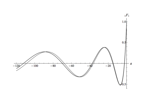
Figure 1: Plot of the zeros $a_{nL}$ ($n=1,2,3$) of the Kummer function ${}_{1}F_{1}$ for $\Omega_{3}=0$ (solid line) and $\Omega_{3}=0.1$ (dashed line) for the fixed values of parameters $m=1$, $\omega_{0}=0.1$, $\omega=0.5$, $\eta=0.9$ and $L=0$.

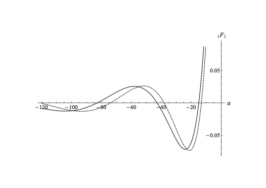
Figure 2: Plot of the zeros $a_{nL}$ ($n=1,2,3$) of the Kummer function ${}_{1}F_{1}$ for $\Omega_{3}=0$ (solid line) and $\Omega_{3}=0.1$ (dashed line) for the fixed values of parameters $m=1$, $\omega_{0}=0.1$, $\omega=1.0$, $\eta=0.5$ and $L=1$.

Tables 1 and 2 correspond to the tables 1 and 2 in Ref. [22]. Castro considered $n=1,\cdots,5$ whereas we took $n=1,2,3$, since we had at least two additional parameters to analyse: $\Omega_{3}$ and $m_{z}$. Our tables elucidate the influence of the cosmic string parameter $\eta\ \in(0,1]$, related both to the string’s linear mass density and to the deficit angle, on the zeros $a_{nL}$ and on the energy eigenvalues ${\mathcal{E}}_{\pm}$.

		$L=0$
		$\Omega_{3}=0$			$\Omega_{3}=0.1$
$\eta$	$n$	$a_{nL}$	$\left|\mathcal{E}_{\pm}\right|$		$a_{nL}$	$\left|\mathcal{E}_{\pm}\right|$
			$m_{z}=0$	$m_{z}=1$		$m_{z}=0$	$m_{z}=1$
0.9	$1$	$-2.4546$	$1.4078$	$1.4771$	$-2.3680$	$1.4069$	$1.4763$
	$2$	$-14.9645$	$2.6431$	$2.6806$	$-14.5051$	$2.6427$	$2.6802$
	$3$	$-37.4516$	$3.9976$	$4.0225$	$-36.3209$	$3.9973$	$4.0223$
0.5	$1$	$-0.4896$	$1.0935$	$1.1814$	$-0.4652$	$1.0899$	$1.1781$
	$2$	$-4.3861$	$1.6596$	$1.7188$	$-4.2478$	$1.6576$	$1.7168$
	$3$	$-11.3311$	$2.3521$	$2.3942$	$-10.9858$	$2.3507$	$2.3928$
0.1	$1$	$0.0000$	$1.0000$	$1.0954$	$0.0000$	$0.8696$	$0.9778$
	$2$	$-1.0000$	$1.1832$	$1.2649$	$-1.0000$	$1.0810$	$1.1698$
	$3$	$-2.0000$	$1.3416$	$1.4142$	$-2.0000$	$1.2573$	$1.3345$

		$L=1$
		$\Omega_{3}=0$					$\Omega_{3}=0.1$
$\eta$	$n$	$a_{nL}$	$\mathcal{E}_{+}$		$\mathcal{E}_{-}$		$a_{nL}$	$\mathcal{E}_{+}$		$\mathcal{E}_{-}$
			$m_{z}=0$	$m_{z}=1$	$m_{z}=0$	$m_{z}=1$		$m_{z}=0$	$m_{z}=1$	$m_{z}=0$	$m_{z}=1$
0.9	$1$	$-7.0092$	$1.5065$	$1.5557$	$-2.5065$	$-2.5557$	$-6.7710$	$1.5060$	$1.5552$	$-2.5060$	$-2.5552$
	$2$	$-25.0484$	$2.8528$	$2.8825$	$-3.8528$	$-3.8825$	$-24.2715$	$2.8525$	$2.8822$	$-3.8525$	$-3.8822$
	$3$	$-53.0832$	$4.2387$	$4.2598$	$-5.2387$	$-5.2598$	$-51.4693$	$4.2385$	$4.2596$	$-5.2385$	$-5.2596$
0.5	$1$	$-2.7840$	$1.0854$	$1.1473$	$-2.0854$	$-2.1473$	$-2.6659$	$1.0835$	$1.1455$	$-2.0835$	$-2.1455$
	$2$	$-9.7150$	$1.7991$	$1.8422$	$-2.7991$	$-2.8422$	$-9.3890$	$1.7977$	$1.8409$	$-2.7977$	$-2.8409$
	$3$	$-19.7364$	$2.5487$	$2.5813$	$-3.5487$	$-3.5813$	$-19.1107$	$2.5476$	$2.5803$	$-3.5476$	$-3.5803$
0.1	$1$	$0.0000$	$1.2321$	$1.2888$	$-2.2321$	$-2.2888$	$0.0000$	$1.1786$	$1.2372$	$-2.1786$	$-2.2372$
	$2$	$-1.0000$	$1.3439$	$1.3973$	$-2.3439$	$-2.3974$	$-1.0000$	$1.2972$	$1.3520$	$-2.2972$	$-2.3520$
	$3$	$-2.0006$	$1.4494$	$1.5001$	$-2.4494$	$-2.5001$	$-2.0003$	$1.4085$	$1.4602$	$-2.4085$	$-2.4602$

Table 1: Values for the roots $a_{nL}$ of the Kummer function $M\left(a_{nL},\frac{L}{\eta},Z_{\text{hw}}\right)=0$ with the fixed values $m=1,$ $\omega_{0}=0.1$ and $\omega=0.5$.

		$L=0$
		$\Omega_{3}=0$			$\Omega_{3}=0.1$
$\eta$	$n$	$a_{nL}$	$\left|\mathcal{E}_{\pm}\right|$		$a_{nL}$	$\left|\mathcal{E}_{\pm}\right|$
			$m_{z}=0$	$m_{z}=1$		$m_{z}=0$	$m_{z}=1$
0.9	$1$	$-11.2177$	$2.3425$	$2.3848$	$-9.9821$	$2.3419$	$2.3842$
	$2$	$-61.2139$	$5.0483$	$5.0681$	$-54.7008$	$5.0481$	$5.0679$
	$3$	$-151.1562$	$7.8398$	$7.8525$	$-135.148$	$7.8397$	$7.8524$
0.5	$1$	$-3.1363$	$1.5015$	$1.5667$	$-2.7572$	$1.4989$	$1.5642$
	$2$	$-18.5757$	$2.9035$	$2.9377$	$-16.5688$	$2.9023$	$2.9365$
	$3$	$-46.3368$	$4.4198$	$4.4424$	$-41.3994$	$4.4190$	$4.4416$
0.1	$1$	$-0.0004$	$1.0001$	$1.0955$	$-0.0001$	$0.8796$	$0.9867$
	$2$	$-1.0238$	$1.1872$	$1.2687$	$-1.0109$	$1.1071$	$1.1940$
	$3$	$-2.2262$	$1.3750$	$1.4458$	$-2.1337$	$1.3145$	$1.3885$

		$L=1$
		$\Omega_{3}=0$					$\Omega_{3}=0.1$
$\eta$	$n$	$a_{nL}$	$\mathcal{E}_{+}$		$\mathcal{E}_{-}$		$a_{nL}$	$\mathcal{E}_{+}$		$\mathcal{E}_{-}$
			$m_{z}=0$	$m_{z}=1$	$m_{z}=0$	$m_{z}=1$		$m_{z}=0$	$m_{z}=1$	$m_{z}=0$	$m_{z}=1$
0.9	$1$	$-31.0448$	$2.6933$	$2.7202$	$-4.6933$	$-4.7202$	$-27.6583$	$2.6930$	$2.7200$	$-4.6930$	$-4.7200$
	$2$	$-103.2043$	$5.5195$	$5.5348$	$-7.5195$	$-7.5348$	$-92.1997$	$5.5193$	$5.5347$	$-7.5193$	$-7.5347$
	$3$	$-215.3445$	$8.3467$	$8.3573$	$-10.3467$	$-10.3574$	$-192.501$	$8.3465$	$8.3572$	$-10.3465$	$-10.3572$
0.5	$1$	$-15.0250$	$1.7221$	$1.7586$	$-3.7221$	$-3.7586$	$-13.2896$	$1.7210$	$1.7575$	$-3.7210$	$-3.7575$
	$2$	$-42.8174$	$3.3043$	$3.3275$	$-5.3043$	$-5.3275$	$-38.1468$	$3.3035$	$3.3267$	$-5.3035$	$-5.3267$
	$3$	$-82.9228$	$4.8795$	$4.8965$	$-6.8795$	$-6.8965$	$-74.0178$	$4.8790$	$4.8960$	$-6.8790$	$-6.8960$
0.1	$1$	$-1.3258$	$\mathbf{0.8789}$	$\mathbf{0.9314}$	$-2.8789$	$-2.9314$	$-0.9500$	$\mathbf{0.8532}$	$\mathbf{0.9064}$	$-2.8532$	$-2.9064$
	$2$	$-4.3039$	$\mathbf{1.1729}$	$\mathbf{1.2185}$	$-3.1729$	$-3.2185$	$-3.55911$	$1.1451$	$\mathbf{1.1912}$	$-3.1451$	$-3.1912$
	$3$	$-7.8222$	$1.4757$	$1.5157$	$-3.4757$	$-3.5157$	$-6.6770$	$1.4486$	$1.4891$	$-3.4486$	$-3.4891$

Table 2: Values for the roots $a_{nL}$ of the Kummer function $M\left(a_{nL},\frac{L}{\eta},Z_{\text{hw}}\right)=0$ with the fixed values $m=1,$ $\omega_{0}=0.1$ and $\omega=1.0$.

For fixed values of $\left\{n,L,m_{z},\Omega_{3}\right\}$, the larger the $\eta$, the smaller the absolute value of both $a_{nL}$ and ${\mathcal{E}}_{\pm}$. If instead, we consider fixed values of the parameters $\left\{n,L,m_{z},\Omega_{3},\eta\right\}$, then the absolute values of $a_{nL}$ and ${\mathcal{E}}_{\pm}$ increase when the parameter $\omega$ goes from $\omega=0.5$ to $\omega=1.0$.

We observe that the effect of non-commutative parameter $\Omega_{3}$ is to decrease the absolute values of $a_{nL}$ and ${\mathcal{E}}_{\pm}$ (for fixed values of the remaining parameters). If we increase the value of $m_{z}$, then the absolute values of ${\mathcal{E}}_{\pm}$ increase. The values of $a_{nL}$ do not depend on $m_{z}$ and remain unchanged. Notice that the hard-wall position $\rho_{0}$ does not depend on $m_{z}$.

We note that the roots $a_{nL}$ and the energies ${\mathcal{E}}_{\pm}$ increase in absolute value as $n$ increases. Finally, let us mention that the effect of $L$ is to increase the absolute value of $a_{nL}$ and ${\mathcal{E}}_{\pm}$ for the great majority of the cases reported in Tables 1 and 2. There are only a few exceptions for $\omega=1.0$; they are highlighted in bold-face numbers in Table 2. This shows that, in general, there is no standard global pattern for the effect of quantum number $L$ on both the roots roots $a_{nL}$ and the energies ${\mathcal{E}}_{\pm}$.

Lastly, we point out that there is consistency between the numerical case of a finite hard-wall and the analytical case in which the hard-wall approaches infinity. Recall that in the latter case, $a_{nL}=-n$. In fact, consider the numerical results for $a_{nL}$ and $\eta=0.1$ in Table 1 for which $\omega=0.5$: it is evident that $a_{nL}$ assumes negative integer values with four digits precision for $L=0$ regardless of the non-commutative parameter. For $L=1$, this is also true up to the third decimal place. These remarks show that $\rho_{0}=1/\omega\eta=20$ (for $\omega=0.5$ and $\eta=0.1$) is already a good approximation to $\rho_{0}\rightarrow\infty$ up to the decimal figures considered in Table 1. This pattern is even more pronounced here than in the commutative case [22] due to the effect of $\Omega_{3}$ on $a_{nL}$.

Figs. 3 and 4 show graphic representations of the information within Tables 1 and 2.

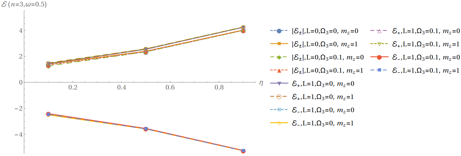
(a)   

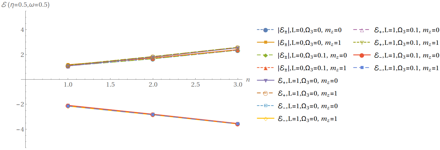
(b)   

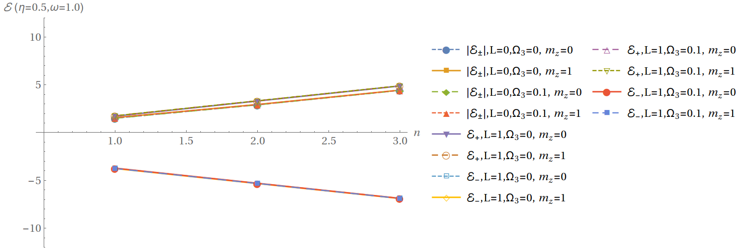
(c)   

Figure 3: Energy eigenvalues ${\mathcal{E}}_{\pm}$ (a) as a function of $\eta$ for $n=3$ and $\omega=0.5$; (b) as a function of $n$ for $\eta=0.5$ and $\omega=0.5$; and, (c) as a function of $n$ for $\eta=0.5$ and $\omega=1.0$.

Fig. 3 displays the effect of the parameters $\eta$, $n$ and $\omega$ on the eigenvalues $\mathcal{E}_{\pm}$. In Part (a), we fix $n=3$ and set $\omega=0.5$ while allowing $\eta=0.1,0.5,0.9$. It enables us to conclude that the absolute value of $\mathcal{E}_{\pm}$ increases with $\eta$. In part (b) we take $\omega=0.5$, $\eta=0.5$ and vary the integer $n$ from 1 to 3. The curves shows that $\left|\mathcal{E}_{\pm}\right|$ increases with the principal quantum number $n$. In part (c), we plot $\mathcal{E}_{\pm}\left(n\right)$ with $\eta=0.5$ and $\omega=1.0$. By comparison of parts (b) and (c) of Fig. 3, we notice that $\left|\mathcal{E}_{\pm}\right|$ increases for increasing values of $\omega$.

Fig. 4 presents the effect of non-commutativity upon our physical system.

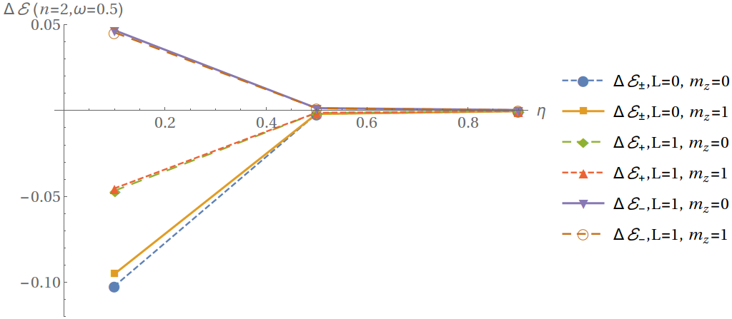
(a)   

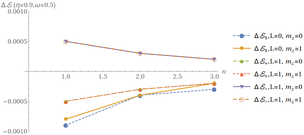
(b)   

Figure 4: Plot of the energy difference $\Delta\mathcal{E}_{\pm}\equiv\mathcal{E}_{\pm}\left(\Omega_{3}=0.1\right)-\mathcal{E}_{\pm}\left(\Omega_{3}=0\right)$ in terms of the string parameter $\eta$ and the principal quantum number $n$: (a) $\Delta\mathcal{E}_{\pm}\left(\eta\right)$ with $n=2$; (b) $\Delta\mathcal{E}_{\pm}\left(n\right)$ with $\eta=0.9$. Both graphs are evaluated with $\omega=0.5$.

The energy difference $\Delta\mathcal{E}_{\pm}$ is defined as the difference of energy calculated at $\Omega_{3}=0.1$ and the corresponding energy at $\Omega_{3}=0$ (commutative case) for fixed values of $n,\,\eta,\,\omega,\,L$ and $m_{z}$, i.e. $\Delta\mathcal{E}_{\pm}\equiv\mathcal{E}_{\pm}\left(\Omega_{3}=0.1\right)-\mathcal{E}_{\pm}\left(\Omega_{3}=0\right)$. In part (a) of Fig. 4 we show how the values of $\Delta\mathcal{E}_{\pm}$ vary with $\eta$ when $n=2$ and $\omega=0.5$ (the several lines correspond to the trends for different values of the remaining parameters). We observe that $\Delta\mathcal{E}_{\pm}$ increases inasmuch the values of $\eta$ decrease. In Fig. 4(b), we display $\Delta\mathcal{E}_{\pm}\left(n\right)$ while setting $\eta=0.9$ and $\omega=0.5$. In this case, the energy difference values decrease with rising values of the quantum number $n$.

To conclude, we are in a position to put into perspective the effect of the coupling prescription which introduces non-commutativity. Let us compare Fig. 4 of this paper with the corresponding Fig. 4 of Paper 1, Ref. [12], which shows how differently the non-commutative parameter $\Omega_{3}$ impacts the DKP-like oscillator in comparison with the KG oscillator. In fact, by comparing the $y$-axis values of the plot in Fig. 4(b) of this paper against the corresponding $y$-axis values of the plot in Fig. 4(b) of Ref. [12], we see that the values of $\left|\Delta\mathcal{E_{\pm}}\left(n\right)\right|$ for the DKP-like oscillator are one order of magnitude smaller than the values of $\left|\Delta\mathcal{E_{\pm}}\left(n\right)\right|$ for the KG oscillator. Thus we are led to conclude that the effect of $\Omega_{3}$ is much more pronounced upon the KG oscillator than it is upon the DKP-like oscillator. In other words, the coupling prescription in Eq. (2) used for the KG oscillator is more powerful than the coupling prescription $\mathbf{p}\rightarrow\ \mathbf{p}-\frac{\boldsymbol{\Omega}\times\mathbf{r}}{2}$ to both $\phi$ and $\phi^{*}$ used for the DKP-like oscillator when it comes down to changing the energy spectrum via non-commutativity.

4 Concluding remarks

Spin-zero fields can be described by either a KG field or a DKP field. The KG field is a solution to a second-order differential equation whereas DKP field satisfies a first-order differential equation. Both KG and DKP descriptions for the spin-zero field are equivalent in the absence of interactions. This equivalence in not necessarily established in the presence of interaction (e.g. with the introduction of the oscillator prescription). In the face of the possibility of non-equivalence, it is fair to ask the question: What is the more adequate description of the spin-zero field? The answer calls for the characterization of both KG and DKP, their different predictions, phenomenology, and coupling prescriptions. This paper studied of the coupling prescription related to a DKP-type of oscillator where the possibility of non-commutativity is also considered.

One of the questions that guided our investigation was the following: Is there a second-order differential equation for the spin-zero field that is (different from the KG description but) equivalent to the DKP formulation? The answer to this question is positive as long as we adopt a coupling prescription for the spin-zero oscillator that is different from the one in Ref. [12]. The difference is materialized through distinct sign choices in the coupling, which were be specified in Section 2.

The introduction of non-commutativity in the momentum space of the DKP-like oscillator leads to new phenomenology, in the sense that a novel wave function is obtained as solution to the field equation with its very own energy spectrum. This was thoroughly discussed here. Moreover, we were able to show the equivalence to Castro’s DKP oscillator of Ref. [22] in the commutative limit.

Here, we continued work done in Part 1 (in Ref.[12]) and examined the spin-zero DKP-like oscillator in a rotating frame with a cosmic string space-time endowed with non-commutative geometry in the momentum space, in order to assess the effects of these geometrical structures. As far as we know, our two papers are the first investigation of this generalized Klein-Gordon equation with non-commutative geometry. We looked for time-independent solutions in cylindrical coordinates and restricted the study to one non-zero non-commutativity parameter, $\Omega_{3}$, along the cosmic string axis. We introduced the oscillator in analogy with the Dirac oscillator of Ref. [14], and solved the resulting three-dimensional equation by implementing the separation of variables in terms of radial distance $\rho$, azimuth $\varphi$ and axial coordinate $z$.

The azimuthal function takes the familiar form in terms of the angular momentum quantum number $L$ of Eq. (26), whereas the axial coordinate sector is, unsurprisingly, expressed in terms of the Hermite polynomials, which are familiar solutions of the quantum harmonic oscillator. The most intricate sector of the solution concerns the radial coordinate which, after considering the asymptotic behaviours at the origin and at infinity, involves the confluent hypergeometric function of the first kind, or Kummer function. From these radial solutions, we obtained the energy quantization by taking into account the hard-wall condition in the limit where $\rho_{0}=\frac{1}{\omega\eta}$ approached infinity, as well as for a finite value of $\rho_{0}$. For the hard-wall at infinity, we obtained an expression for the energy eigenvalues in terms of a principal quantum number $n$ as well of various physical parameters. We discussed various limits for these parameters and observed various couplings between physical quantities. Among others, we noticed that the non-commutativity parameter $\Omega_{3}$ may reduce or enhance the energy values, depending on other parameters. For the hard-wall at finite distance from the cosmic string, we performed a numerical search of the roots of the Kummer function in terms of various parameters. We were able to compare our results, in the commutative limit, with Ref. [22] whose author also studied the non-inertial effects on the dynamics of scalar boson, but by solving the Duffin-Kemmer-Petiau oscillator. Among many other observations, we noticed that the non-commutativity parameter $\Omega_{3}$ reduces the absolute value of the energy. Since we solved the three-dimensional spatial problem, we thus extend the analysis in Ref. [22], including in the commutative limit. Other papers on similar topics restrict their analysis to the plane $z=0$, including the energy quantization. We did not impose this restriction nor its additional implications on the wave function and energy spectrum.

Finally, we compare the results of the present paper with those of Part 1. This allows us to analyze the role of the coupling prescriptions in each case (Eqs.(1),(2) in Part 1 and Eqs.(5),(15) in Part 2). Several points can be highlighted. Firstly, we compare the axial part of the solution, $Z(z)$: In Part 1, a Gaussian function is obtained as solution, while here, the Gaussian function is multiplied by a Hermite polynomial. This is a significant difference, since in the latter, the separation constant is quantized; in the former, the separation constant $K$ remains arbitrary. Concerning the radial solution, the definition of the dimensionless variable $\xi\equiv S\rho$, with $S$ given by Eq. (35) in the present paper, led to an equation that could be solved analytically, without approximations. The solution ended up being, essentially, a Gaussian multiplied by a Kummer function. In Part 1, the same definition for the dimensionless variable resulted in a dissipative system with an imaginary rest mass in the non-relativisitic limit. There, this problem was solved with a different choice of dimensionless variable, where the non-commutative parameter took no part in. The result was an equation that could be solved only perturbatively, leading to a solution given by a Gaussian multiplied by a Whittaker function. As a consequence, the resulting energy presented a very distinct behaviour. The analytical expression for the quantized energy in Part 1 showed that the absolute value of energy decreases with the quantum number $n$; here, this same quantity increases with this parameter. When the numerical values for the quantized energy were obtained, the effect of the non-commutative parameter in Part 1 was to increase the absolute value of energy in comparison with the commutative case; here, the energy decreases. All these differences stemmed from the coupling prescription adopted for each case.

Our initial interest in the behaviour of a spin-zero oscillator in cosmic string backgrounds stems from the influence of topological defects in cosmology. In the context of particle physics, our investigation of the Klein-Gordon equation clearly helps to describe the motion of scalar bosons, such as pions, in the presence of a cosmic string. Our results can be also of interest in condensed matter physics, given the general connections between particle physics phenomena (such as topological defects, cosmic strings or spontaneous symmetry breaking) and linear topological defects in solids, such as (edge, screw) dislocations or (wedge, twist) disclinations. Non-commutative geometry has had a resurgence of interest among particle physicists about twenty years ago, mainly due to a paper by Seiberg and Witten who argued that the coordinate functions of the endpoints of strings constrained to a D-brane in the presence of a constant Neveu-Schwarz B-field would satisfy a non-commutative algebra [32, 33, 34]. The work [35] by Bigatti and Susskind considers non-commutativity in the context of string theory in the presence of a D3-brane and a constant large magnetic field. Afterwards there were studies of the quantum Hall effect on non-commutative spaces [36, 37, 39], so that possible applications in condensed matter systems include the quantum Hall effect for interacting bosons as a example of a symmetry-protected topological phase, as in Refs. [40, 41, 42], although considering the effects of topological defects and non-commutative geometry. Finally, another class of applications could concern Bose-Einstein condensation along the lines of Refs. [43, 44] which employed the formalism of the Duffin-Kemmer-Petiau theory (equivalent to KG for spinless field) in the relativistic and Galilean cases, respectively. For instance, the angular velocity necessary for a rotating Bose-Einstein condensate for the formation of vortices, as in Refs. [45, 46] could be influenced by the non-commutativity parameter.

References

- [1] S. Weinberg, The Quantum Theory of Fields vol. 1 Foundations, (Cambridge Univ. Press, Cambridge, 1995)
- [2] R.J. Duffin, Phys. Rev. 54 (1938) 1114
- [3] N. Kemmer, Proc. R. Soc. A 173 (1939) 91
- [4] G. Petiau, Thesis: Contribution á la théorie des équations d’ondes corpusculaires, Acad. R. Belg. Cl. Sci. Mém. Collect. 8 (1936) 16, No 2
- [5] W. Greiner, Relativistic Quantum Mechanics - Wave Equations 3rd Ed. (Springer, Heidelberg, 2000)
- [6] E. Friedman and G. Kalbermann, Phys. Rev. C 34 (1986) 2244
- [7] Y. Yang, H. Hassanabadi, H. Chen, Z.W. Long, Int. J. Mod. Phys. E 30 (2021) 2150050
- [8] J.T. Lunardi, B.M. Pimentel, R.G. Teixeira, J.S. Valverde, Phys. Lett. A 268 (2000) 165
- [9] R. Utiyama, Phys. Rev. 101 (1956) 1597
- [10] R.F. Guertin, T.L. Wilson, Phys. Rev. D 15 (1977) 1518
- [11] B. Vijayalakshmi, M. Seetharaman, P.M. Mathews, J. Phys. A: Math. Gen. 12 (1979) 665
- [12] R.R. Cuzinatto, M. de Montigny, P.J. Pompeia, Non-commutativity and non-inertial effects on a scalar field in a cosmic string space-time - Part 1: Klein-Gordon oscillator
- [13] R.R. Cuzinatto, M. de Montigny, P. J. Pompeia, Gen. Relat. Grav. 51 (2019) 107
- [14] M. Moshinsky and A. Szczepaniak, J. Phys. A: Math. Gen. 22 (1989) L817
- [15] K. Bakke, Gen. Relativ. Gravit. 45 (2013) 1847
- [16] Y. Nedjadi, R.C. Barrett, J. Phys. A Math. Gen. 27 (1994) 4301
- [17] F. Delduc, Q. Duret, F. Gieres, M. Lefrancois, J. Phys. Conf. Ser. 103 (2008) 012020
- [18] H. Hassanabadi, M. Hosseinpour, Eur. Phys. J. C 76 (2016) 553
- [19] M. Hosseinpour, H. Hassanabadi, M. de Montigny, Eur. Phys. J. C 79 (2019) 311
- [20] H. Chen, Z.W. Long, Q.K. Ran, Y. Yang, C.Y. Long, EPL, 132 (2020) 50006
- [21] Y. Yang, Z.W. Long, Q.K. Ran, H. Chen, Z.L. Zhao, C.Y. Long, Int. J. Mod. Phys. A 36 (2021) 2150023
- [22] L.B. Castro, Eur. Phys. J. C 76 (2016) 61
- [23] M. Hosseinpour, H. Hassanabadi, F. M. Andrade, Eur. Phys. J. C 78 (2018) 93
- [24] M. Hosseinpour, H. Hassanabadi, Adv. High Energy Phys. 2018 (2018) 2959354
- [25] D.J. Griffiths, Introduction to Quantum Mechanics, 2nd ed. (Pearson, Upper Saddle River, 2005)
- [26] L. Schiff, Quantum Mechanics, 3rd ed. (McGraw-Hill, New York, 1968)
- [27] G. Sagnac, Comptes Rendus Acad. Sci. 157 (1913) 708
- [28] G. Sagnac, Comptes Rendus Acad. Sci. 157 (1913) 1410
- [29] L.A. Page, Phys. Rev. Lett. 35 (1975) 543
- [30] S.A. Werner, J.L. Staudenmann, R. Colella, Phys. Rev. Lett. 42 (1979) 1103
- [31] Wolfram Research, Inc., Mathematica, Version 10, Champaign, IL (2014)
- [32] A. Connes, M.R. Douglas, A. Schwartz, J. High Energy Phys. 02 (1998) 003
- [33] M.R. Douglas, C. Hull, J. High Energy Phys. 02 (1998) 008
- [34] N. Seiberg, E. Witten, J. High Energy Phys. 09 (1999) 032
- [35] D. Bigatti and L. Susskind Phys. Rev. D 62 (2000) 066004
- [36] O.F. Dayi, A. Jellal, J. Math. Phys. 43 (2002) 4592 [Erratum 45 (2004) 827]
- [37] B. Basu, S. Ghosh, Phys. Lett. A 346 (2005) 133
- [38] A.L. Carey, K. Hannabuss, V. Mathai, J. Geom. Sym. Phys. 6 (2006) 16
- [39] B. Harms, O. Micu, J. Phys. A 40 (2007) 10337
- [40] T. Senthil, M. Levin, Phys. Rev. Lett. 110 (2013) 046801
- [41] A. Sterdyniak, N.R. Cooper, N. Regnault, Phys. Rev. Lett. 115 (2015) 116802
- [42] T. Senthil, Annu. Rev. Condens. Matter Phys. 6 (2015) 299
- [43] R. Casana, V.Ya. Fainberg, B.M. Pimentel, J.S. Valverde, Phys Lett. A 316 (2003) 33
- [44] L.M. Abreu, A.L. Gadelha, B.M. Pimentel, E.S. Santos, Physica A 419 (2015) 612
- [45] G. Baym, C. J. Pethick, Phys, Rev. Lett. 76 (1996) 6
- [46] E. Lundh, C.J. Pethick, H. Smith, Phys. Rev. A 55 (1997) 2126