Double Source Lensing Probing High Redshift Cosmology

Abstract

Double source lensing, with two sources lensed by the same foreground galaxy, involves the distance between each source and the lens and hence is a probe of the universe away from the observer. The double source distance ratio also reduces sensitivity to the lens model and has good complementarity with standard distance probes. We show that using this technique at high redshifts $z>1$, to be enabled by data from the Euclid satellite and other surveys, can give insights on dark energy, both in terms of $w_{0}$–$w_{a}$ and redshift binned density. We find a dark energy figure of merit of 245 from combination of 256 double source systems with moderate quality cosmic microwave background and supernova data. Using instead five redshift bins between $z=1.1$–5, we could detect the dark energy density out to $z\approx 5$, or make measurements ranging between 31$\sigma$ and 2.5$\sigma$ of its values in the bins.

I Introduction

Gravitational lensing gives a visual manifestation of general relativity in the universe, deflecting light from distance sources by foreground mass concentrations. When the lensing is strong, multiple images occur, with angular separations determined by the Einstein radius combining the lens mass with a “focal length” involving distances between the source, lens, and observer. In the particular situation of multiple sources lensed by the same mass, generally known as double source plane lensing (DSPL), the ratio of Einstein radii or deflection angles measured by image separations involves a pure distance ratio; the impact of the lens mass profile details – modeling this can be a significant source of uncertainty in strong lensing – is much reduced collett12 ; collett14 (also see schneider ).

Moreover, the key distance ratio is a purely geometric probe, reflecting the cosmic expansion history separate from the growth history uncertainties, and involves distances between the source and lens, removed from the observer, i.e. probing the distant universe separated from the local universe. Furthermore it is independent of the Hubble constant $H_{0}$. This offers the interesting possibility of exploring the Hubble parameter and matter-energy contents of the universe at redshifts far from the observer, and with different covariances than other distances.

Previous studies of the cosmological leverage of image separations and DSPL linder04 ; collett12 ; collett14 ; linder16 showed useful complementarity with other lensing probes, strengthening their dark energy figure of merit by $\sim 40\%$. Those investigations focused on lens redshifts $z\leq 0.6$. Here we consider higher redshift systems, as will be enabled soon by the Euclid satellite euclid1 ; euclid2 ; euclid3 , and later by proposed higher redshift surveys such as MegaMapper megamapper and others snowhi . We also explore complementarity with standard distance probes, and go beyond the standard dark energy equation of state redshift dependence and allow dark energy density to vary freely in bins of redshift, testing for “early” dark energy behavior at $z\approx 1$–5.

One could also go beyond galaxy-galaxy-galaxy (one lens, two sources) lensing to use the cosmic microwave background (CMB) as a source plane 1605.05337 , or go beyond probing expansion history to look at effects of modified gravitational potentials on the deflection angles 1906.06324 , although we do not address those here.

In Section II we investigate the sensitivity of the DSPL distance ratio to cosmological parameters, showing that it exhibits unique properties relative to other distance probes. Section III propagates this to projected parameter estimation uncertainties, for various redshift ranges of observations and combinations with other data. In Section IV we study the impact of the source redshift distribution. We explore early dark energy constraints in Section V, allowing independent redshift bins of dark energy density, and summarize, discuss, and conclude in Section VI.

II Cosmological Sensitivity of DSPL

The critical surface mass density for strong lensing involves the distance ratio $r_{s}/(r_{l}r_{ls})$ of distances between source and observer, lens and observer, and source and lens, respectively. The ratio of light deflection angles (or Einstein radii when the lens mass factor cancels out) for two sources with a common lens is the ratio of distance ratios, and the central quantity for DSPL,

$$\beta(z,z_{1},z_{2}) \equiv \frac{r_{ls}(z,z_{1})}{r_{s}(z_{1})}\frac{r_{s}(z_{2})}{r_{ls}(z,z_{2})}$$ (1)

$$= \frac{D_{ls}(z,z_{1})}{D_{s}(z_{1})}\frac{D_{s}(z_{2})}{D_{ls}(z,z_{2})}\ .$$ (2)

where the lens is at redshift $z$, the nearer source is at $z_{1}$, and the further source at $z_{2}$. Here $r(z,z_{i})$ is the angular distance to redshift $z_{i}$ seen by an observer at redshift $z$, with the single argument $r(z_{i})$ indicating the distance is measured from redshift zero, and

$$D(z,z_{i})=\int_{z}^{z_{i}}\frac{dz^{\prime}}{H(z^{\prime})}\,$$ (3)

is the conformal distance for a flat universe as we will use. Note that $\beta$ is the same whether using angular or conformal distances, as long as all the distances are treated consistently. Conformal distances in a flat universe have the convenient property that $D(z,z_{i})=D(z_{i})-D(z)$.

We consider measurements of $\beta$ from observed image positions of strong lensing systems. Since Einstein radii involve lens mass factors as well, the ratio formed from image separations or positions is not strictly a function of distance only, except in special cases like a point mass or singular isothermal sphere lens profile. However, the dependence on lens mass profile (and its uncertainties, including substructure, and mass sheet degeneracies) is expected to be suppressed for DSPL relative to other uses of lensing; see collett12 ; collett14 ; 23inLin2016 ; schneider ; 25inLin2016 . Also, we focus on galaxy lenses, where any residual mass effects could be modeled more easily. Nevertheless, followup high resolution mapping (and possibly spectroscopy) of the lens will be an important adjunct. For a few hundred lenses this should not be a major observational program.

Deep, wide field surveys such as that from the Euclid satellite (and less deep from the Vera C. Rubin Observatory’s Legacy Survey of Space and Time (LSST lsst ) and less wide but higher resolution from the Nancy Grace Roman Space Telescope roman ) should find hundreds of DSPL. Even focusing on the best observed systems should deliver a data set of $\sim 160$ from Euclid, potentially doubling when adding in other surveys 23inLin2016 ; 26inLin2016 ; 27inLin2016 ; lenspop ; 1803.03604 ; oh ; 2010.15173 .

We emphasize that we do not employ the abundance or distribution of lensed systems as a cosmological probe, which would involve a complicated blend of cosmology and survey characteristics and selection functions. Rather, we use the properties of individual systems and, in the manner of time delay (single source plane) lenses, we can use a data set of the best observed systems.

The sensitivity of the measured $\beta$ to cosmological parameters is calculated through the partial derivatives, as a fractional change relative to some measurement precision, $(\partial\beta/\partial\theta)/\sigma(\beta)$. The cosmological parameters $\theta$ we use are $\Omega_{m}$, the matter density today as a fraction of the critical density, and initially the dark energy equation of state parameters $w_{0}$ and $w_{a}$, describing its present value and a measure of its time variation. We take a flat $\Lambda$CDM universe with fiducial values $\Omega_{m}=0.3$, $w_{0}=-1$, $w_{a}=0$. For illustration purposes we adopt a single measurement precision of 1%, $\sigma(\beta)=0.01\beta$, and show $\beta(z,z_{1},z_{2})$ and its derivatives for fixed $z_{1}/z=2$, $z_{2}/z_{1}=1.5$. These ratios correspond roughly to the peak of the lensing “focal length” kernel, i.e. the most efficient and hence most commonly detected. Variations of these ratios were explored in linder16 and will be here as well in Section IV, after the next, motivational paragraph. Moreover, we will find in Section IV, where we vary the redshift ratios, that this fiducial choice (basically the lower envelope in Figure 1) will give the most conservative dark energy constraints (figure of merit) – actual data may well give more advantageous leverage.

While there are very few DSPL currently known, we can explore the reasonableness of the redshift ratio $z_{\rm source}/z_{\rm lens}\approx 2$, motivated by the lensing kernel, for known standard strong lenses. Figure 1 plots the redshift ratio for 1842 galaxy-galaxy and 117 quasar-galaxy strong lenses where the source and lens redshifts have been measured brownstein . We see that indeed the value $z_{\rm source}/z_{\rm lens}\approx 2$ is a reasonable approximation. In Section IV we will quantify the impact on our results if we alter this.

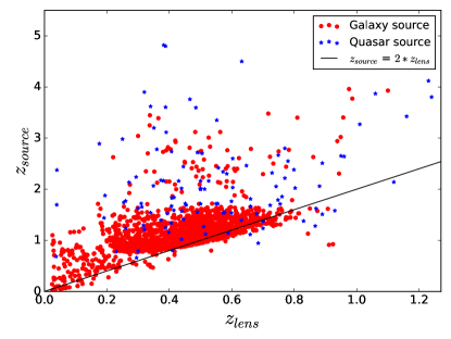
Figure 1: For known galaxy lens systems, the distribution of $z_{\rm source}$ vs $z_{\rm lens}$ is reasonably approximated by $z_{\rm source}=2\,z_{\rm lens}$. Data are extracted from brownstein .

A nice property of $\beta$ for the conditions given is that $\beta$ is nearly constant for a wide range of redshifts. Hence there is negligible difference between taking an absolute measurement precision or a fractional measurement precision. The 1% fiducial fractional precision for measurement of $\beta$ will depend on survey properties, though it is likely to be a conservative choice. For example, collett14 in 2014 achieved 1.1% fractional precision on $\beta$; the subsequent improvement in telescopes and instrumentation, and the development of, e.g. machine learning, tools for finding and measuring lens systems may indicate that better than 1% will be achieved. While we stay with the conservative choice, we note that parameter constraints from the lensing data alone will scale linearly with the statistical precision, while somewhat more slowly when external data such as CMB data is included.

Our results (from $\beta$, without other data) will scale with the precision.

Figure 2 illustrates $\beta$ as a function of lens redshift, showing its near constancy, with deviations remaining less than 1% out to $z_{\rm lens}=2$. The limit as $z\equiv z_{\rm lens}\to 0$ is readily calculable as $\beta\to(1-z/z_{1})/(1-z/z_{2})$, or 0.75 for our fiducial values. If we took $z_{2}\to z_{1}$ we would get $\beta\to 1$, while if $z_{2}\gg z_{1}=2z$ then $\beta\to 0.5$.

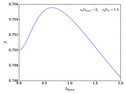
Figure 2: Double source plane lensing distance ratio $\beta$ is nearly constant as a function of lens redshift $z_{\rm lens}$.

Figure 3 presents the cosmological parameter sensitivities, following linder16 but extending the results to much higher redshift than considered there. This shows several new interesting properties. Between $z\approx 1.6$–2.5 the $\beta$ observable has greater sensitivity to $w_{a}$ than to $w_{0}$ – highly unusual among cosmological probes. At $z\approx 2.1$, there is a null to the influence of $w_{0}$, which could potentially relieve covariance between parameters. As the shapes of the sensitivity curves differ between parameters, we expect high redshift measurements in general to aid in breaking covariances.

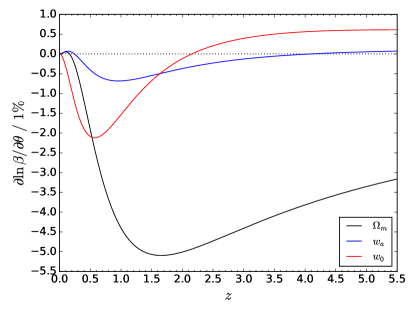
Figure 3: The sensitivity of measurements of the double source lensing distance ratio $\beta$ for constraining cosmological parameters $\theta$ is plotted as a function of the lens redshift $z$. The magnitude of the sensitivity is here for a 1% measurement of $\beta$, but the more interesting aspects come from the shape of the curves: the null of the $\Omega_{m}$ curve at $z\approx 0.15$ and the opposite signs for $w_{0}$ and $w_{a}$ sensitivities for $z\leq 0.23$, as well as $w_{a}$ becoming more sensitive than $w_{0}$ at $z\approx 1.6$, and the null of the $w_{0}$ curve at $z\approx 2.1$, indicating distinct behaviors from single distance probes.

III Cosmological Leverage of DSPL

The information matrix formalism presents an efficient method for combining the sensitivities, taking into account their covariances, and the measurement uncertainties, to obtain cosmological parameter constraints. We will initially focus on the dark energy equation of state space, $w_{0}$–$w_{a}$, marginalizing over the matter density. To begin with, we consider how observations at different redshifts affect the constraints.

Figure 4 shows that the covariance direction of the constraints in the $w_{0}$–$w_{a}$ space rotates as the lens redshift $z$ increases (keeping the relations $z_{1}/z=2$, $z_{2}/z_{1}=1.5$). This is clearest when fixing $\Omega_{m}$, as shown by the solid contours becoming vertical (strong $w_{0}$ constraints) near the $w_{a}$ sensitivity null at $z\approx 0.23$, and horizontal (strong $w_{a}$ constraints) near the $w_{0}$ sensitivity null at $z\approx 2.1$. However the steady rotation (and hence complementarity between different redshifts) holds when marginalizing over $\Omega_{m}$ (as we do throughout the article), as shown by the dotted contours. In order to obtain closed contours, we take three observations clustered around the labeled redshift, i.e. at $z$, $z\pm 0.05$.

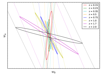
Figure 4: The leverage of measurements of the double source lensing distance ratio $\beta$ for constraining the dark energy equation of state value today $w_{0}$ and time variation $w_{a}$ is plotted for observations focused at different lens redshifts $z$. Note the rotation of the covariance direction, indicating good complementarity over a range of redshifts. Solid ellipses fix $\Omega_{m}=0.3$ for clarity while dotted ellipses (extending off the plot) marginalize over $\Omega_{m}$. Since the focus is on covariance direction near a single redshift, we omit the scale due to idealized precision.

We see that higher redshift measurements are expected to have good complementarity with lower redshift ones. Thus the upcoming generation of high redshift surveys such as Euclid can contribute significantly to dark energy constraints through the DSPL probe. For detailed constraints, we study three redshift ranges, roughly corresponding to three depths of surveys, for $z=[0.1,0.6]$, $[0.6,1.1]$, and $[1.1,1.6]$, each range divided into six bins of width 0.1, e.g. with bin centers at $z=0.1$, 0.2, …, 0.6. While even higher redshifts could be useful, using $z_{\rm lens}>1.6$ would correspond to both $z_{\rm source}\gtrsim 3$, making observations more difficult and time consuming. In each redshift bin we assume 16 DSPL each with $\beta$ measured to 1% (treated statistically, i.e. any systematics common across systems are below the 1% level). This corresponds to 96 DSPL per set, a reasonable “gold set” for upcoming surveys.

Figure 5 shows the dark energy constraints, and figure of merit FOM$=\sqrt{\det F(w_{0},w_{a})}$, where $F$ is the information matrix. We always marginalize over $\Omega_{m}$, and combine different redshift ranges of DSPL with external information in the form of a Planck prior on the distance to last scattering of the cosmic microwave background (CMB). For each individual redshift range of DSPL, plus CMB, the dark energy constraints are not particularly tight – this is because the unique virtue of DSPL in depending on the higher redshift universe through $D_{ls}$ actually means the constraints are weaker in the low redshift range where dark energy dominates. However we will shortly see that also including a low redshift standard distance probe, such as Type Ia supernova distances (SN), will allow the unique leverage of DSPL to work.

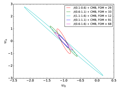
Figure 5: 1$\sigma$ joint confidence contours on $w_{0}$–$w_{a}$ for DSPL over various redshift ranges, plus CMB. Note the strong complementarity of including DSPL all the way out to $z=1.1$.

The low and middle redshift ranges for DSPL give nearly equivalent FOM when combined with CMB. The high redshift range is much weaker, since its covariance direction (see Fig. 4) is nearly the same as that for CMB. Again, the situation will change significantly when we later add a standard distance probe as well. Combining complementarity redshift ranges for DSPL indeed has a strong effect: for the low+mid redshift combination, FOM increases by a factor 3, while mid+high redshift gives a factor 2 increase (again not as strong due to overlap in covariance direction with CMB).

Now let us add supernovae (one could equally well use distances from baryon acoustic oscillations). We use a moderate projected sample (same as in linder16 ), with SN concentrated at $z<1$, specifically 150 local ($z<0.1$), 900 between $z=0.1$–1, and 42 over $z=1$–1.7. While Euclid does not include a SN survey (but see desire ), LSST will obtain many at $z\lesssim 1$, though without spectroscopy; the 900 used can be thought of as systematics dominated in the SN magnitude measurement, at $dm=0.02(1+z)/2.7$ mag; we marginalize over the SN effective absolute magnitude $\mathcal{M}$. As mentioned above, the inclusion of a standard distance probe giving just $D(z)$ enables the leverage of DSPL on $D_{ls}(z,z^{\prime})$ to have great effect.

Figure 6 displays the cosmological constraints from DSPL measurements over various redshift ranges, plus combinations of ranges, when including both CMB and SN. Now the high redshift set of DSPL gives the best constraints, with FOM=176, a factor 15 improvement over without SN. By contrast the low and mid redshift DSPL cases improve by a factor $\sim 4$. When combining low and mid redshift DSPL (and CMB), SN still adds an improvement of a factor 1.9 over the case without SN from Fig. 5. All three DSPL redshift ranges (so 256 systems total, still a reasonable number) would give FOM=245, compared to FOM=72 from CMB+SN without DSPL, i.e. a factor 3.4 improvement. The 1$\sigma$ marginalized uncertainties for the case $\beta(0.1-1.6)$+CMB+SN are $\sigma(\Omega_{m})$ = 0.0058, $\sigma(w_{0})$ = 0.059, $\sigma(w_{a})$ = 0.20.

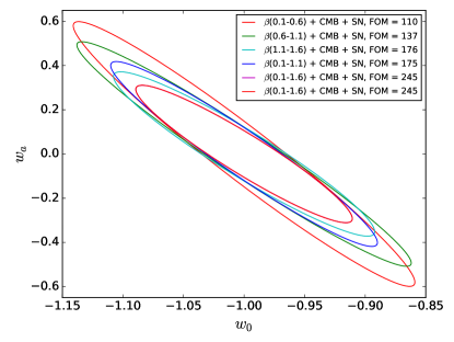
Figure 6: 1$\sigma$ joint confidence contours on $w_{0}$–$w_{a}$ for DSPL over various redshift ranges, plus CMB and SN. Note the complementarity of DSPL with both CMB and SN, leading to increased figures of merit.

IV Source Redshift Distribution

To check the robustness of the results, we revisit variation of the relations $z_{1}/z=2$ and $z_{2}/z_{1}=1.5$. We compute the effects on the dark energy FOM as a function of these ratios over all lens redshifts, allowing the ranges $z_{1}/z=[1.1,3]$ and $z_{2}/z_{1}=[1.1,3]$. The second source redshift $z_{2}$ however is not allowed to exceed $z_{2}=5$, due to the difficulty in finding such systems owing to faintness and reduced galaxy formation rate.

Figure 7 shows contours of FOM in the $z_{1}/z$ – $z_{2}/z_{1}$ plane, for the combination of data sets that in Fig. 6 gave FOM=245: $\beta(0.1-1.6)$+CMB+SN. Variation of $z_{1}/z$ within the range 1.5–2.5 has a rather modest effect, changing the FOM by less than 10%, while even $z_{1}/z=3$ only affects FOM at the 20% level. For $z_{2}/z_{1}$, our fiducial value is quite a conservative choice, with $z_{2}/z_{1}=2$ (2.5) improving FOM by 40% (60%), raising FOM over 340. Thus DSPL can be a significant contributor to probing the nature of dark energy.

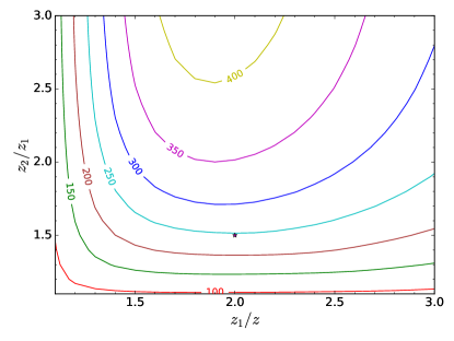
Figure 7: FOM isocontours for $\beta(0.1-1.6)$+CMB+SN, with a $z_{2}\leq 5$ cut imposed. The star in the figure represents the fiducial ratios $z_{1}/z=2$, $z_{2}/z_{1}=1.5$, giving FOM = 245 as in Fig. 6.

V Exploring High Redshift Dark Energy Density

Advantageous characteristics of DSPL as a cosmic probe include the relatively good sensitivity at high redshift and the capability to explore the expansion at redshifts between the lens and source redshifts through $D_{ls}$, rather than all the way from the observer including the local universe. As well, $D_{ls}$ gives the benefit of complementarity with standard $D(z)$ probes. Therefore we investigate what DSPL can tell us about high redshift dark energy, beyond the usual $w_{0}$–$w_{a}$ parametrization.

In this section dark energy density is allowed to float freely within high redshift bins, to see how the data can constrain dark energy at the epochs when it is predicted to be at the 1–20% level of the critical energy density within the $\Lambda$CDM model. That is, we take as parameters $\Omega_{m}$, $\{\Omega_{\rm de}(z_{i})\}$, employing five bins with $z_{i}$ being the centers of $z=[1.1,1.4]$, [1.4,1.7], [1.7,2], [2,2.5], [2.5,5]. See also 2106.09581 ; 2106.09713 for other probes constraining binned high redshift dark energy density.

We employ the combined data set as in Fig. 6 and Fig. 7: $\beta(0.1-1.6)$+CMB+SN. Figure 8 shows the $1\sigma$ marginalized uncertainty band on the dark energy density as a function of redshift, across the five bins. We see that the uncertainty band is distinct from zero dark energy density out to $z\approx 5$ (at 68% CL). The magnitudes of the $1\sigma$ marginalized uncertainties are $\sigma(\Omega_{m})=0.0028$, $\sigma(\Omega_{\rm de}(z_{i}))=0.0055$, 0.0082, 0.011, 0.0071, 0.0084 respectively. This would correspond to 31, 15, 8.4, 9.0, $2.5\sigma$ evidence for dark energy at $z=1.25$, 1.55, 1.85, 2.25, 3.75 respectively. (The constraints weaken for bins at higher redshift as dark energy is less dynamically important there, then strengthen in the last two bins that we chose to be broader.)

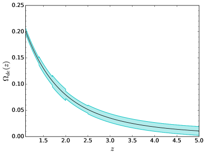
Figure 8: Constraints on high redshift dark energy density enabled by observations of $\beta(0.1-1.6)$+CMB+SN are shown as a shaded band (68% CL) around the $\Lambda$CDM fiducial behavior (black curve). The presence of dark energy could be detected out to $z\approx 5$ (at 68% CL).

Figure 9 presents a corner plot of the 2D joint confidence contours for the high redshift binned dark energy density parameters, plus the present matter density. The combination of data breaks degeneracies significantly, as seen by the substantially circular contours, leaving the greatest correlation coefficient as $0.88$ between the present matter density and the dark energy density in the highest ($z_{5}$) bin. Thus the combination of DSPL, involving $D_{ls}$, and standard distance measures $D(z)$ such as from supernovae (or baryon acoustic oscillations), plus CMB, is a powerful probe of dark energy in the high redshift universe as well.

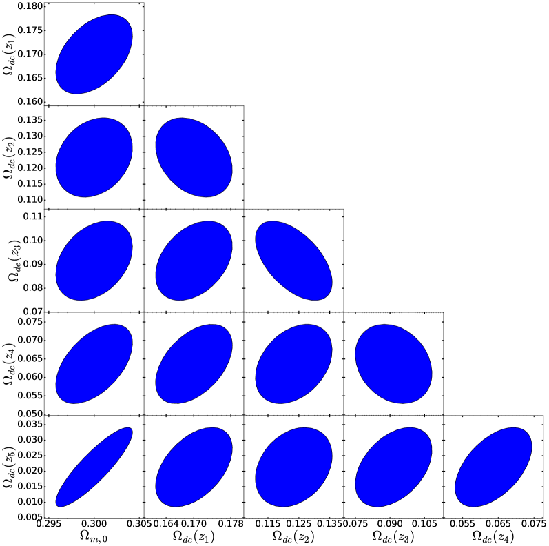
Figure 9: 2D joint 68% CL constraints on high redshift dark energy density and the present matter density enabled by observations of $\beta(0.1-1.6)$+CMB+SN indicate the power and complementarity of DSPL for probing dark energy even at high redshift.

VI Conclusions

Additional methods for probing cosmology and the nature of dark energy to complement and enhance the standard techniques would be highly valuable. Double source plane lensing offers several promising characteristics, including hundreds of expected detections and measurements from the Euclid satellite and other surveys, intriguing dependence on the “remote” distance between lens and source without local universe dependence, and strong complementarity between low and high redshift observations and with standard distance measures.

We have quantified the cosmological leverage of DSPL in terms of both constraints on dark energy equation of state parameters $w_{0}$, $w_{a}$, and figure of merit and on freely varying binned dark energy density at high redshift. The first demonstrates that DSPL, together with moderate level CMB and supernovae data, can give FOM $\approx 250$, rising to $\approx 350$ for a less conservative source redshift distribution. The second shows that DSPL can be a superb probe of the high redshift universe, detecting nonzero dark energy density out to $z\approx 5$ and giving several statistically significant measures of dark energy in independent redshift bins between $z\approx 1.1$–5.

Complementarity between cosmic probes – to break degeneracies, crosscheck results, and guard against systematics – is valuable, between $D_{ls}$ and $D(z)$, between low and high redshift, and between DSPL and strong gravitational lensing time delays. Strong gravitational lensing should become a significant, mature technique with the upcoming generation of wide surveys, and the extension to the $z\gtrsim 2$ universe with Euclid and future instruments adds a new, further frontier.

These are exciting prospects, and upcoming surveys should keep DSPL as a science case as they develop detection pipelines, assess the numbers predicted by 23inLin2016 ; 26inLin2016 ; 27inLin2016 ; lenspop ; 1803.03604 ; oh ; 2010.15173 , and carry out observations. High redshift spectroscopic instruments such as MegaMapper will play a critical role in measuring source redshifts and for modeling the lens mass profile to see its residual impact on the $\beta$ distance ratio. Overall, DSPL could provide an important addition to methods for understanding the cosmic expansion history.

- (1) T.E. Collett, M.W. Auger, V. Belokurov, P.J. Marshall, A.C. Hall, Constraining the dark energy equation of state with double source plane strong lenses, MNRAS 424, 2864 (2012) [arXiv:1203.2758]
- (2) T.E. Collett, M.W. Auger, Cosmological Constraints from the double source plane lens SDSSJ0946+1006, MNRAS 443, 969 (2014) [arXiv:1403.5278]
- (3) P. Schneider, Can one determine cosmological parameters from multi-plane strong lens systems?, Astron. Astroph. 568, L2 (2014) [arXiv:1406.6152]
- (4) E.V. Linder, Strong Gravitational Lensing and Dark Energy Complementarity, Phys. Rev. D 70, 043534 (2004) [arXiv:astro-ph/0401433]
- (5) E.V. Linder, Doubling Strong Lensing as a Cosmological Probe, Phys. Rev. D 94, 083510 (2016) [arXiv:1605.04910]
- (6) R. Laureijs et al., Euclid Definition Study Report, arXiv:1110.3193
- (7) G.D. Racca et al., Euclid mission design, Proc. SPIE 9904, 99040O (2016) [arXiv:1610.05508]
- (8) R. Scaramella et al., Euclid preparation: I. The Euclid Wide Survey, arXiv:2108.01201
- (9) D.J. Schlegel et al., MegaMapper: a spectroscopic instrument for the study of Inflation and Dark Energy, arXiv:1907.11171
- (10) S. Ferraro, N. Sailer, A. Slosar, M. White, Cosmology and Fundamental Physics from the three-dimensional Large Scale Structure, arXiv:2203.07506
- (11) H. Miyatake, M.S. Madhavacheril, N. Sehgal, A. Slosar, D.N. Spergel, B. Sherwin, A. van Engelen, Measurement of a Cosmographic Distance Ratio with Galaxy and Cosmic Microwave Background Lensing, Phys. Rev. Lett. 118, 161301 (2017) [arXiv:1605.05337]
- (12) D. Jyoti, J.B. Muñoz, R.R. Caldwell, M. Kamionkowski, Cosmic time slip: Testing gravity on supergalactic scales with strong-lensing time delays, Phys. Rev. D 100, 043031 (2019) [arXiv:1906.06324]
- (13) R. Gavazzi, T. Treu, L.V.E. Koopmans, A.S. Bolton, L.A. Moustakas, S. Burles, P.J. Marshall, The Sloan Lens ACS Survey. VI. Discovery and Analysis of a Double Einstein Ring, ApJ 677, 1046 (2008) [arXiv:0801.1555]
- (14) P. Schneider, Generalized shear-ratio tests: A new relation between cosmological distances, and a diagnostic for a redshift-dependent multiplicative bias in shear measurements, Astron. Astroph. 592, L6 (2016) [arXiv:1603.04226]
- (15) LSST Dark Energy Science Collaboration, LSST Dark Energy Science Collaboration (DESC) Science Requirements Document, arXiv:1809.01669
- (16) O. Doré et al., WFIRST: The Essential Cosmology Space Observatory for the Coming Decade, arXiv:1904.01174
- (17) T.E. Collett, The Population of Galaxy-Galaxy Strong Lenses in Forthcoming Optical Imaging Surveys, ApJ 811, 20 (2015) [arXiv:1507.02657]
- (18) T.E. Collett, private communication
- (19) M.S. Talbot et al., SDSS-IV MaNGA: The Spectroscopic Discovery of Strongly Lensed Galaxies, MNRAS 477, 195 (2018) [arXiv:1803.03604]
- (20) S. Oh, Hierarchical Bayesian scheme for measuring the properties of dark energy with Strong gravitational lensing, arXiv:1804.02637
- (21) T.E. Collett, github.com/tcollett/LensPop
- (22) C. Weiner, S. Serjeant, C. Sedgwick, Predictions for Strong Lens Detections with the Nancy Grace Roman Space Telescope, Res. Notes AAS 4, 190 (2020) [arXiv:2010.15173]
- (23) Main Lens Database http://admin.masterlens.org
- (24) P. Astier et al., Extending the supernova Hubble diagram to with the Euclid space mission, Astron. Astroph. 572, A80 (2014) [arXiv:1409.8562]
- (25) E.V. Linder, The Rise of Dark Energy, arXiv:2106.09581
- (26) N. Sailer, E. Castorina, S. Ferraro, M. White, Cosmology at high redshift – a probe of fundamental physics, JCAP 2112, 049 (2021) [arXiv:2106.09713]