Constraining New Physics with Borexino Phase-II spectral data

Abstract

We present a detailed analysis of the spectral data of Borexino Phase II, with the aim of exploiting its full potential to constrain scenarios beyond the Standard Model. In particular, we quantify the constraints imposed on neutrino magnetic moments, neutrino non-standard interactions, and several simplified models with light scalar, pseudoscalar or vector mediators. Our analysis shows perfect agreement with those performed by the collaboration on neutrino magnetic moments and neutrino non-standard interactions in the same restricted cases and expands beyond those, stressing the interplay between flavour oscillations and flavour non-diagonal interaction effects for the correct evaluation of the event rates. For simplified models with light mediators we show the power of the spectral data to obtain robust limits beyond those previously estimated in the literature.

1 Introduction

The scattering among electrons and neutrinos played an important historical role in the establishment of the Standard Model (SM) allowing for precise tests of the V-A structure of the weak interactions. Being a purely weak, purely leptonic, two-body reaction, makes both the theoretical cross-section calculation and the experimental signatures particularly clean. The scattering of $\nu_{\mu,\tau}$ on electrons is a purely weak neutral-current (NC) process, while $\nu_{e}\,e^{-}$ scattering proceeds via both weak NC and weak charged-current (CC) interactions. The latter is of particular interest because it is one of the few reactions for which the SM predicts a large destructive interference between these two channels. For the same reasons it is a sensitive probe of physics beyond the Standard Model (BSM). Paradigmatic examples include neutrino electromagnetic properties, non-standard neutrino-matter interactions (NSI), and new interactions mediated by light bosons. Most precise results on $\nu_{\mu}\,e^{-}\to\nu_{\mu}\,e^{-}$ were obtained by the CHARM-II experiment CHARM-II:1993phx , while $\nu_{e}\,e^{-}\to\nu_{e}\,e^{-}$ was first observed with an accelerator beam in the experiment performed at LAMPF Allen:1992qe , followed by the measurement at the LSND experiment LSND:2001akn . Since the pioneering work of Reines and collaborators Reines:1976pv the scattering process $\bar{\nu}_{e}\,e^{-}\to\bar{\nu}_{e}\,e^{-}$ has been studied at a greater level of precision using neutrinos produced in nuclear reactors Vidyakin:1992nf ; Derbin:1993wy ; MUNU:2005xnz , most recently in the TEXONO TEXONO:2006xds and GEMMA experiments Beda:2012zz ; Beda:2013mta . Neutrino electron elastic scattering (ES) can also be searched for at experiments designed to detect Coherent Elastic neutrino-Nucleus Scattering (CE$\nu$NS): while the signal in the SM would be too low to yield a significant number of events, the presence of BSM physics may lead to much larger contributions. In fact, CE$\nu$NS searches using reactor neutrinos at the CONUS CONUS:2020skt ; Rink:2022rsx , CONNIE CONNIE:2019xid , and Dresden-II reactor experiments Colaresi:2022obx ; Coloma:2022avw lead to very strong constraints on some of the BSM scenarios outlined above. Similar searches can be performed using pion decay-at-rest (DAR) sources: for example, the data of the COHERENT experiment on CsI COHERENT:2017ipa should be sensitive to an ES signal as well Coloma:2022avw since it would pass their signal selection cuts.

Neutrino electron elastic scattering is also key to the study of solar neutrinos. Solar neutrinos were first detected in real time through ES scattering in water in Kamiokande Kamiokande-II:1989hkh . In fact, the observed rate of ES versus CC interactions allowed for the first model-independent evidence of flavour transitions in solar neutrinos in Super-Kamiokande and SNO Super-Kamiokande:1998qwk ; SNO:2001kpb . For the last 15 years the Borexino Borexino:2000uvj experiment has been detecting ES of solar neutrinos in liquid scintillator performing precision spectroscopy of their energy spectrum at Earth Borexino:2008dzn ; Borexino:2017rsf ; BOREXINO:2020aww . The main purpose of the experiment was the independent determination of the fluxes produced by the different thermonuclear reactions in the Sun. Nevertheless, the precision of their high-statistics spectral data also allows for precision tests of ES and, as such, it has been used by the collaboration itself Borexino:2017fbd ; Borexino:2019mhy . Borexino results have also been analyzed/adapted by phenomenological groups to impose bounds on BSM scenarios (see, e.g., Refs. Bilmis:2015lja ; Harnik:2012ni ; Agarwalla:2012wf ; Khan:2019jvr ; deGouvea:2009fp ; Amaral:2020tga ; Montanino:2008hu ; Brdar:2017kbt ; Khan:2017djo ; Khan:2017oxw for an incomplete list), in general using either total event rates or early spectral data.

In this work we present a detailed analysis of the spectral data of Borexino Phase II with the aim of exploiting its full potential to constrain new physics which can significantly affect ES (such as neutrino magnetic moments, NSI, and simplified models with light scalar, pseudoscalar, and vector mediators). In general BSM scenarios, neutrino neutral-current interactions may be flavour changing. This brings the issue of the interplay between neutrino oscillations and interactions which do not conserve the neutrino flavour, which has not always been properly treated in previous literature on this topic. Section 2 presents the formalism to correctly evaluate the event rates, accounting for flavour oscillations in presence of flavour non-diagonal interactions (details are also presented in Appendix A). This section also introduces the interaction cross sections for the BSM models considered. Section 3 contains the description of our calculation of the expected spectra at Borexino and the dataset used, as well as our treatment of backgrounds, uncertainties and further details on the statistical analysis. It is complemented with Appendix B.

The main results of our work are presented in Sec. 4. As mentioned above, the Borexino collaboration has already performed two analyses on BSM searches using a spectral fit of the Phase-II data set: a first analysis which is used to set constraints on the neutrino magnetic moment Borexino:2017fbd , and a later search for NSI with electrons Borexino:2019mhy . As we will show in Sec. 4, our results are in excellent agreement with those obtained in Ref. Borexino:2017fbd for the magnetic moment scenario: this serves as validation for our $\chi^{2}$ construction and, in particular, for the implementation of systematic uncertainties (a key point in this analysis, given the large number of events collected by Borexino). Regarding NSI, our analysis expands over the results obtained in Ref. Borexino:2017fbd in two main ways: (i) we include all NSI operators in neutrino flavour space at once in the fit, thus allowing for potential correlation effects and cancellations in the cross section; and (ii) we consider four different cases regarding the structure of the operators (vector, axial vector, left-handed only, and right-handed only). Finally, our work includes the derivation of new constraints for simplified models with new light vector, scalar, and pseudoscalar mediators, which to the best of our knowledge have not been reported by the collaboration yet. Finally, we summarize our conclusions in Sec. 5.

2 Theoretical Frameworks

In the SM, the differential cross section for neutrino-electron ES ($\nu_{\beta}\,e^{-}\to\nu_{\beta}\,e^{-}$) can be expressed as Bahcall:1995mm

$$\dfrac{\mathrm{d}\sigma^{\text{SM}}_{\beta}}{\mathrm{d}T_{e}}(E_{\nu},T_{e})=\dfrac{2G_{F}^{2}m_{e}}{\pi}\bigg{\{}c_{L\beta}^{2}\Big{[}1+\dfrac{\alpha}{\pi}f_{-}(y)\Big{]}+c_{R\beta}^{2}\,(1-y)^{2}\Big{[}1+\dfrac{\alpha}{\pi}f_{+}(y)\Big{]}\\ -2\,c_{L\beta}\,c_{R\beta}\,\dfrac{m_{e}y}{2E_{\nu}}\Big{[}1+\dfrac{\alpha}{\pi}f_{\pm}(y)\Big{]}\bigg{\}}\,,$$ (1)

where $T_{e}$ stands for electron (kinetic) recoil energy, $E_{\nu}$ is the neutrino energy, and $y\equiv T_{e}/E_{\nu}$, and $f_{+}$, $f_{-}$, $f_{\pm}$ are loop functions given in Ref. Bahcall:1995mm , while $\alpha$ stands for the fine-structure constant, $G_{F}$ is the Fermi constant, and $m_{e}$ is the electron mass. The effective couplings $c_{L\beta}$ and $c_{R\beta}$ contain the contributions from the SM NC, which are equal for all flavours, plus the CC contribution which only affects $\nu_{e}e^{-}$ scattering:

$$c_{Le} =\rho\,\Big{[}\kappa_{e}(T_{e})\sin^{2}\theta_{w}-\dfrac{1}{2}\Big{]}+1\,, \quad c_{Re} =\rho\,\kappa_{e}(T_{e})\sin^{2}\theta_{w}\,,$$ (2)

$$c_{L\tau}=c_{L\mu} =\rho\,\Big{[}\kappa_{\mu}(T_{e})\sin^{2}\theta_{w}-\dfrac{1}{2}\Big{]}\,, \quad c_{R\tau}=c_{R\mu} =\rho\,\kappa_{\mu}(T_{e})\sin^{2}\theta_{w}\,,$$

with $\rho$ and $\kappa_{\beta}(T_{e})$ departing from $1$ due to radiative corrections of the gauge boson self-energies and vertices Bahcall:1995mm . The minimum neutrino energy required to produce an electron with a given recoil energy $T_{e}$ is $E_{\nu,\text{min}}=\big{(}T_{e}+\sqrt{T_{e}^{2}+2\,m_{e}\,T_{e}}\,\big{)}\big{/}2$, while the maximum kinetic energy for an electron produced by a neutrino with given energy $E_{\nu}$ is $T_{e,\text{max}}=E_{\nu}^{2}\big{/}(E_{\nu}+m_{e}/2)$. The corresponding cross section for $\bar{\nu}_{\beta}\,e^{-}$ ES can be obtained from (1) with the exchange $c_{L\beta}\leftrightarrow c_{R\beta}$.

We assume that scattering off electrons is incoherent, so for the calculation of the number of events it is enough to multiply the total cross section $\sigma^{\text{SM}}_{\beta}(E_{\nu})$ – obtained by integrating Eq. (1) over $T_{e}$ – by the overall number of electrons in the fiducial volume. In principle, a correction factor taking into account that the target electrons are actually bound to atoms have to be considered for recoil energies comparable to atomic binding energies. However, for the solar neutrino energies considered here this effect can be safely neglected.

Solar neutrinos produced in the core of the Sun are purely $\nu_{e}$. Propagation through vacuum and matter induces a non-trivial evolution of their flavour, so that neutrinos reaching the detector are in general not definite flavour eigenstates but rather a coherent superposition of them, which can be described in terms of the elements $S_{\beta e}$ of an unitary matrix $S$ (see Appendix A). As discussed above, in the SM the ES cross section includes contributions from both CC interactions (which are diagonal in the flavour basis) and NC interactions (which are diagonal in any basis), so that the flavour basis is the most adequate to describe them. The common approach consists in projecting the neutrino state at the detector over the flavour eigenstates, thus introducing the $\nu_{e}\to\nu_{\beta}$ transition probabilities $P_{e\beta}\equiv|S_{\beta e}|^{2}$, and then convoluting them with the cross sections for pure flavour states given in Eq. (1). So the number of interactions of solar neutrinos in Borexino will be proportional to the probability-weighted electron scattering cross section:

$$N_{\text{ev}}\propto\sum_{\beta}P_{e\beta}\,\sigma^{\text{SM}}_{\beta}\,.$$ (3)

This well-known expression relies on the special role played in the SM by the flavour basis, which as we have seen diagonalizes both CC and NC interactions. However, through this work we will consider several BSM phenomenological scenarios leading to modifications of the interaction cross section in Eq. (1). When the BSM is not lepton-flavour conserving, the CC-defined flavour basis may no longer correspond to the NC eigenstates, and extra care must be taken with the interplay of oscillations and scattering. To address this issue, it is convenient to rewrite Eq. (3) in a basis-independent form:

$$N_{\text{ev}}\propto\operatorname{Tr}\Big{[}\rho^{(e)}\,\sigma^{\text{SM}}\Big{]}\,,$$ (4)

where $\rho^{(e)}\equiv S\,\Pi^{(e)}S^{\dagger}$ is the density matrix of the neutrino state at the detector, with $\Pi^{(e)}$ being the projector on the electron neutrino flavour at the source. Here $\sigma^{\text{SM}}$ is a generalized cross section, i.e., a matrix in flavour space which contains enough information to describe the ES interaction of any neutrino state without the need to explicitly project it onto the interaction eigenstates. Such projection is now implicitly encoded into $\sigma^{\text{SM}}$, which in the flavour basis takes the diagonal form $\sigma^{\text{SM}}_{\gamma\beta}=\delta_{\gamma\beta}\,\sigma^{\text{SM}}_{\beta}$. In the same basis we have $\rho_{\beta\gamma}^{(e)}=S_{\beta e}S_{\gamma e}^{*}$, so that $\rho_{\beta\beta}^{(e)}=P_{e\beta}$ and Eq. (3) is immediately recovered. Let us stress that the indexes $\gamma\beta$ in $\sigma^{\text{SM}}_{\gamma\beta}$ do not make reference to “initial” and “final” states of the scattering process but they are both initial flavour indexes, just as the indexes of $\rho_{\beta\gamma}^{(e)}$ both refer to the final state of the neutrino as it reaches the detector.

2.1 Neutrino Non-Standard Interactions with Electrons

The so-called non-standard neutrino interaction (NSI) framework consists on the addition of four-fermion effective operators to the SM Lagrangian at low energies. For example, the effective Lagrangian

$$\mathcal{L}_{\text{NSI,NC}}=-2\sqrt{2}G_{F}\sum_{f,P,\alpha,\beta}\varepsilon_{\alpha\beta}^{f,P}(\bar{\nu}_{\alpha}\gamma^{\mu}P_{L}\nu_{\beta})(\bar{f}\gamma_{\mu}Pf)\,,$$ (5)

would lead to new NC interactions with the rest of the SM fermions. Here $P$ can be either a left-handed or a right-handed projection operator ($P_{L}$ or $P_{R}$, respectively) and the matrices $\varepsilon_{\alpha\beta}^{f,P}$ are hermitian: $\big{(}\varepsilon_{\beta\alpha}^{f,P}\big{)}^{*}=\varepsilon_{\alpha\beta}^{f,P}$. The index $f$ refers to SM fermions and in what follows we will be focusing on $f=e$. Such new interactions may induce lepton flavour-changing processes (if $\alpha\neq\beta$), or may lead to a modified interaction rate with respect to the SM result (if $\alpha=\beta$). For later convenience we also define the vector and axial SM couplings:

$$c_{V\beta}\equiv c_{L\beta}+c_{R\beta}\,,\qquad c_{A\beta}\equiv c_{L\beta}-c_{R\beta}\,,$$ (6)

as well as the corresponding NSI coefficients:

$$\varepsilon_{\alpha\beta}^{f,V}\equiv\varepsilon_{\alpha\beta}^{f,L}+\varepsilon_{\alpha\beta}^{f,R}\,,\quad\varepsilon_{\alpha\beta}^{f,A}\equiv\varepsilon_{\alpha\beta}^{f,L}-\varepsilon_{\alpha\beta}^{f,R}\,.$$ (7)

The presence of flavour-changing effects implies that the SM flavour basis no longer coincides with the interaction eigenstates. In such case the number of events in Borexino will be given by Eq. (4) in terms of a generalized cross section $\sigma^{\text{NSI}}(E_{\nu})$ defined as the integral over $T_{e}$ of the following matrix expression:

$$\dfrac{\mathrm{d}\sigma^{\text{NSI}}}{\mathrm{d}T_{e}}(E_{\nu},T_{e})=\dfrac{2G_{F}^{2}m_{e}}{\pi}\bigg{\{}C_{L}^{2}\Big{[}1+\dfrac{\alpha}{\pi}f_{-}(y)\Big{]}+C_{R}^{2}\,(1-y)^{2}\Big{[}1+\dfrac{\alpha}{\pi}f_{+}(y)\Big{]}\\ -\big{\{}C_{L},C_{R}\big{\}}\,\dfrac{m_{e}y}{2E_{\nu}}\Big{[}1+\dfrac{\alpha}{\pi}f_{\pm}(y)\Big{]}\bigg{\}}\,,$$ (8)

which is formally identical to Eq. (1) except that the $c_{L\beta}$ and $c_{R\beta}$ real coefficients have been superseded by the $3\times 3$ hermitian matrices $C_{L}$ and $C_{R}$:

$$C_{\alpha\beta}^{L}\equiv c_{L\beta}\,\delta_{\alpha\beta}+\varepsilon_{\alpha\beta}^{e,L}\quad\text{and}\quad C_{\alpha\beta}^{R}\equiv c_{R\beta}\,\delta_{\alpha\beta}+\varepsilon_{\alpha\beta}^{e,R}\,.$$ (9)

It is immediate to see that, if the NSI terms $\varepsilon_{\alpha\beta}^{e,L}$ and $\varepsilon_{\alpha\beta}^{e,R}$ are set to zero, the matrix $\mathrm{d}\sigma^{\text{NSI}}\big{/}\mathrm{d}T_{e}$ becomes diagonal and the SM expressions are recovered. The corresponding cross section for $\bar{\nu}_{\beta}\,e^{-}$ ES can be obtained from Eq. (8) with the exchange $C_{L}\leftrightarrow C_{R}^{*}$.

In addition to scattering effects, the presence of NSI also affects neutrino propagation from production to detection point through its contribution to the matter potential both in the Sun and in the Earth. The formalism follows the approach described in Sec. 2.3 of Ref. Esteban:2018ppq . The details of the calculation of the density matrix $\rho^{(e)}$ are provided in Appendix A.

2.2 Neutrino Magnetic-Moments

In the presence of a neutrino magnetic moment ($\mu_{\nu}$) the scattering cross sections on electrons get additional contributions which do not interfere with the SM ones. Neutrino magnetic moments arise in a variety of BSM models and, in particular, they do not need to be flavour-universal. Therefore, in what follows we will allow different magnetic moments for the different neutrino flavours – albeit still imposing that they are flavour-diagonal. Under this assumption the ES differential cross section for either neutrinos or antineutrinos, up to order $\mathcal{O}(y^{2})$, takes the form Vogel:1989iv

$$\frac{\mathrm{d}\sigma^{\mu_{\nu}}_{\beta}}{\mathrm{d}T_{e}}=\frac{\mathrm{d}\sigma^{\text{SM}}_{\beta}}{\mathrm{d}T_{e}}+\left(\frac{\mu_{\nu_{\beta}}}{\mu_{B}}\right)^{2}\frac{\alpha^{2}\,\pi}{m_{e}^{2}}\left[\frac{1}{T_{e}}-\frac{1}{E_{\nu}}\right].$$ (10)

Since no flavour-changing contributions are present in this case, the expression for the number of interactions in Borexino will be just proportional to the probability weighted total cross section, in analogy with Eq. (3).

2.3 Models with light scalar, pseudoscalar, and vector mediators

We also consider simplified models describing the neutrino interaction with fermions of the first generation through a neutral scalar $\phi$, pseudoscalar $\varphi$, or a neutral vector $Z^{\prime}$. Concerning the scalar, the Lagrangian we consider is Cerdeno:2016sfi

$$\mathcal{L}_{\phi}=g_{\phi}\,\phi\bigg{(}q_{\phi}^{e}\,\bar{e}e+\sum_{\alpha}q_{\phi}^{\nu_{\alpha}}\,\bar{\nu}_{\alpha,R}\,\nu_{\alpha,L}+\text{h.c.}\bigg{)}-\frac{1}{2}\,M^{2}_{\phi}\,\phi^{2}\,,$$ (11)

where $q_{\phi}^{j}$ are the individual scalar charges and $j=\{\nu_{\alpha},e\}$. The corresponding cross section for neutrino-electron (or antineutrino-electron) scattering is

$$\frac{\mathrm{d}\sigma_{\beta}^{\phi}}{\mathrm{d}T_{e}}=\frac{\mathrm{d}\sigma^{\text{SM}}_{\beta}}{\mathrm{d}T_{e}}+\frac{g_{\phi}^{4}\,(q^{\nu_{\beta}}_{\phi})^{2}\,(q^{e}_{\phi})^{2}\,m_{e}^{2}\,T_{e}}{4\pi\,E_{\nu}^{2}\,(2\,m_{e}\,T_{e}+M_{\phi}^{2})^{2}}\left(1+\frac{T_{e}}{2\,m_{e}}\right),$$ (12)

where we have included all orders in $T_{e}/E_{\nu}$ and $T_{e}/m_{e}$ (beyond the leading-order terms given in Ref. Cerdeno:2016sfi ), since these are non-negligible for solar event rates at Borexino.

For the pseudoscalar scenario, we consider the Lagrangian

$$\mathcal{L}_{\varphi}=i\,g_{\varphi}\,\varphi\bigg{(}q_{\varphi}^{e}\,\bar{e}\gamma^{5}e+\sum_{\alpha}q_{\varphi}^{\nu_{\alpha}}\,\bar{\nu}_{\alpha,R}\gamma^{5}\nu_{\alpha,L}+\text{h.c.}\bigg{)}-\frac{1}{2}\,M^{2}_{\varphi}\,\varphi^{2}\,,$$ (13)

where $q_{\varphi}^{j}$ are the individual pseudoscalar charges and $j=\{\nu_{\alpha},e\}$. The corresponding cross section for neutrino-electron (or antineutrino-electron) scattering is

$$\frac{\mathrm{d}\sigma_{\beta}^{\varphi}}{\mathrm{d}T_{e}}=\frac{\mathrm{d}\sigma^{\text{SM}}_{\beta}}{\mathrm{d}T_{e}}+\frac{g_{\varphi}^{4}\,(q^{\nu_{\beta}}_{\varphi})^{2}\,(q^{e}_{\varphi})^{2}\,m_{e}\,T_{e}^{2}}{8\pi\,E_{\nu}^{2}\,(2\,m_{e}\,T_{e}+M_{\varphi}^{2})^{2}}\,.$$ (14)

As for the vector mediator, our assumed Lagrangian is:

$$\mathcal{L}_{V}=g_{Z^{\prime}}\,Z^{\prime}_{\mu}\bigg{(}q_{Z^{\prime}}^{e}\,\bar{e}\gamma^{\mu}e+\sum_{\alpha}q_{Z^{\prime}}^{\nu_{\alpha}}\,\bar{\nu}_{\alpha,L}\gamma^{\mu}\nu_{\alpha,L}\bigg{)}+\frac{1}{2}M^{2}_{Z^{\prime}}{Z^{\prime}}^{\mu}Z^{\prime}_{\mu}\,,$$ (15)

with the individual vector charges $q_{Z^{\prime}}^{j}$. Unlike for the scalar and magnetic-moment cases, a neutral vector interaction interferes with the SM contribution. The differential cross section for neutrino-electron scattering reads Lindner:2018kjo

$$\frac{\mathrm{d}\sigma_{\beta}^{Z^{\prime}}}{\mathrm{d}T_{e}}=\frac{\mathrm{d}\sigma^{\text{SM}}_{\beta}}{\mathrm{d}T_{e}}+\frac{g^{2}_{Z^{\prime}}\,m_{e}}{2\,\pi}\Bigg{\{}\frac{g^{2}_{Z^{\prime}}\,(q_{Z^{\prime}}^{\nu_{\beta}})^{2}\,(q^{e}_{Z^{\prime}})^{2}}{\big{(}2m_{e}T_{e}+M_{Z^{\prime}}^{2}\big{)}^{2}}\left[1-\frac{m_{e}\,T_{e}}{2\,E_{\nu}^{2}}+\frac{T_{e}}{2\,E_{\nu}}\left(\frac{T_{e}}{E_{\nu}}-2\right)\right]\\ +\frac{2\sqrt{2}\,G_{F}\,q_{Z^{\prime}}^{\nu_{\beta}}\,q_{Z^{\prime}}^{e}}{\big{(}2m_{e}T_{e}+M_{Z^{\prime}}^{2}\big{)}}\left[c_{V\beta}\left(1-\frac{m_{e}\,T_{e}}{2\,E_{\nu}^{2}}\right)+c_{R\beta}\,\frac{T_{e}}{E_{\nu}}\left(\frac{T_{e}}{E_{\nu}}-2\right)\right]\Bigg{\}}\,,$$ (16)

where $c_{V\beta}$ is the SM effective vector coupling introduced in Eq. (6). For the sake of simplicity, in our calculations describing the effects of light mediators, we have neglected the small SM radiative corrections to the BSM contributions. The corresponding cross section for $\bar{\nu}_{\beta}\,e^{-}$ ES can be obtained from (16) with the exchange $c_{L\beta}\leftrightarrow c_{R\beta}$.

Similarly to the SM and the magnetic moment cases, no flavour-changing contributions are considered for scalar, pseudoscalar, or vector mediators, hence the number of interactions in Borexino will be just proportional to the probability-weighted total cross section as in Eq. (3).

In Sec. 4 we study the constraints on four specific models with light mediators. For scalar and pseudoscalar mediators we will focus on a model in which the mediator couples universally to fermions. For vector mediators we will show the results for three anomaly-free models coupling to electrons, namely $B-L$, $L_{e}-L_{\mu}$ and $L_{e}-L_{\tau}$. For convenience Tab. 1 lists the relevant charges.

Model	$q^{e}$	$q^{\nu_{e}}$	$q^{\nu_{\mu}}$	$q^{\nu_{\tau}}$
Universal/leptonic scalar (or pseudoscalar)	$\hphantom{+}1$	$\hphantom{+}1$	$\hphantom{+}1$	$\hphantom{+}1$
$B-L$ vector	$-1$	$-1$	$-1$	$-1$
$L_{e}-L_{\mu}$ vector	$\hphantom{+}1$	$\hphantom{+}1$	$-1$	$\hphantom{+}0$
$L_{e}-L_{\tau}$ vector	$\hphantom{+}1$	$\hphantom{+}1$	$\hphantom{+}0$	$-1$

Table 1: Charges for the vector, scalar, and pseudoscalar mediators considered in this work.

3 Analysis of Borexino Phase-II Spectrum

In order to constrain the BSM scenarios for neutrino interactions described in Sec. 2 we have performed an analysis of the Borexino Phase-II data collected between December 14th, 2011 and May 21st, 2016, (corresponding to a total exposure of $1291.51~{}\text{days}\times 71.3~{}\text{tons}$) following closely the details presented by the collaboration in Ref. Borexino:2017rsf . In particular we use the spectrum data presented in Fig. 7 of such work which we analyze using the total number of detected hits ($N_{h}$) on the detector photomultipliers (including multiple hits on the same photomultiplier) as estimator of the recoil energy of the electron scattered by the incoming neutrinos. We statistically confront the spectral data with the expected event rates in the different scenarios, which we compute as follows.

Borexino phase-II detects interactions of solar neutrinos produced in the pp, pep, $\mbox{}^{7}\text{Be}$, and $\mbox{}^{8}\text{B}$ reactions of the pp-chain, as well as from all reactions in the CNO-cycle. The produced total flux is described by the differential spectrum:

$$\frac{\mathrm{d}\phi_{\nu}^{\text{prod}}}{\mathrm{d}E_{\nu}}=\sum_{f}\frac{\mathrm{d}\phi_{\nu}^{f}}{\mathrm{d}E_{\nu}}(E_{\nu}),$$ (17)

where $E_{\nu}$ is the neutrino energy and $f$ refers to each of the main components of the solar neutrino flux (pp, pep, CNO, $\mbox{}^{7}\text{Be}$, and $\mbox{}^{8}\text{B}$). In their journey to the Earth the produced $\nu_{e}$ will change flavour and interact upon arrival via elastic scattering with the $e^{-}$ of the detector. Thus, the expected number of solar neutrino events corresponding to $N_{h}$ hits is given by the convolution of the oscillated solar neutrino spectrum with the interaction cross section and the energy resolution function. Quantitatively we compute the solar neutrino signal $S_{i}$ in the $i$-th bin (i.e., with $N_{h}\in[N_{h,\text{min}}^{i},N_{h,\text{max}}^{i}]$) as:

$$S_{i}=\int_{N_{h,\text{min}}^{i}}^{N_{h,\text{max}}^{i}}\int\frac{\mathrm{d}S}{\mathrm{d}T_{e}}(T_{e})\,\frac{\mathrm{d}\mathcal{R}}{\mathrm{d}N_{h}}(T_{e},N_{h})\,\mathrm{d}T_{e}\,\mathrm{d}N_{h}\,.$$ (18)

Here, $\mathrm{d}S\big{/}\mathrm{d}T_{e}$ is the differential distribution of neutrino-induced events as a function of recoil energy of the scattered electrons ($T_{e}$)

$$\frac{\mathrm{d}S}{\mathrm{d}T_{e}}(T_{e})=\mathcal{N}_{\text{tgt}}\,\mathcal{T}_{\text{run}}\,\mathcal{E}_{\text{cut}}\int\frac{\mathrm{d}\phi_{\nu}^{\text{prod}}}{\mathrm{d}E_{\nu}}(E_{\nu})\operatorname{Tr}\left[\rho^{(e)}(E_{\nu})\,\frac{\mathrm{d}\sigma^{X}}{\mathrm{d}T_{e}}(E_{\nu},T_{e})\right]\mathrm{d}E_{\nu}\,,$$ (19)

where $X\in\{\text{SM, NSI, $Z^{\prime}$, $\phi$, $\varphi$, $\mu_{\nu}$}\}$ for the different scenarios discussed in Sec. 2. Note that our notation explicitly reflects that $\mathrm{d}\sigma\big{/}\mathrm{d}T_{e}$ may not be diagonal in flavour space (as in the case of NSI, see the discussion in Sec. 2). In our analysis we fix the oscillation parameters to the best-fit values from Ref. Esteban:2020cvm ; nufit . Here $\mathcal{N}_{\text{tgt}}$ is the number of $e^{-}$ targets, that is, the total number of electrons inside the fiducial volume of the detector (corresponding to 71.3 ton of scintillator), while $\mathcal{T}_{\text{run}}=1291.51~{}\text{days}$ is the data taking time, and $\mathcal{E}_{\text{cut}}=98.5\%$ is the overall efficiency. In addition Eq. (18) includes the energy resolution function $\mathrm{d}\mathcal{R}\big{/}\mathrm{d}T_{e}$ for the detector which gives the probability that an event with electron recoil energy $T_{e}$ yields an observed number of hits $N_{h}$. We assume it follows a Gaussian distribution

$$\frac{\mathrm{d}\mathcal{R}}{\mathrm{d}N_{h}}(T_{e},N_{h})=\frac{1}{\sqrt{2\pi}\,\sigma_{h}(T_{e})}\exp\bigg{[}-\frac{1}{2}\bigg{(}\frac{N_{h}-\bar{N}_{h}(T_{e})}{\sigma_{h}(T_{e})}\bigg{)}^{2}\bigg{]}\,,$$ (20)

where $\bar{N}_{h}$ is the expected value of $N_{h}$ for a given true recoil energy $T_{e}$. We determine $\bar{N}_{h}(T_{e})$ and $\sigma_{h}(T_{e})$ via the calibration procedure described in Appendix B.1.

The data contains background contributions from a number of sources. The main backgrounds come from radioactive isotopes in the scintillator $\mbox{}^{14}\text{C}$, $\mbox{}^{11}\text{C}$, $\mbox{}^{10}\text{C}$, $\mbox{}^{210}\text{Po}$, $\mbox{}^{210}\text{Bi}$, $\mbox{}^{85}\text{Kr}$, and $\mbox{}^{6}\text{He}$. The collaboration identifies two additional backgrounds due to pile-up of uncorrelated events, and residual external backgrounds (see Ref. Borexino:2017rsf for a complete description of these backgrounds).

Among the considered backgrounds, the one coming from $\mbox{}^{11}\text{C}$ is particularly relevant for the analysis. This isotope is produced in the detector by muons through spallation on $\mbox{}^{12}\text{C}$. In Ref. Borexino:2017rsf the collaboration uses a Three-Fold Coincidence (TFC) method to tag the $\mbox{}^{11}\text{C}$ events, which are correlated in space and time with a muon and a neutron. Thus, they divide the Phase II data set in two samples: one enriched (tagged) and one depleted (subtracted) in $\mbox{}^{11}\text{C}$ events. The separation of the solar neutrino signal (as well as most of the other backgrounds) into these two samples is uncorrelated from the number of hits $N_{h}$. Concretely, the tagged sample picks up $35.72\%$ of the solar neutrino events, while the subtracted sample accounts for the remaining $64.28\%$.

In our analysis we include both sets of data, denoted in what follows by $s=\text{``tagged''}$ or “subtracted”. As for the background, we have read the contribution $B_{s,i}^{c}$ for each component $c$, in each bin $i$, and for each data set $s$ from the corresponding lines in the two panels in Fig. 7 of Ref. Borexino:2017rsf . They are shown for the best-fit normalization of the different background components as obtained by the collaboration, and we take them as our nominal background predictions in the absence of systematics. Altogether the nominal number of expected events $T_{s,i}^{0}$ in some bin $i$ of data sample $s$ is the sum of the neutrino-induced signal and the background contributions:

$$T_{s,i}^{0}=\sum_{f}S_{s,i}^{f}+\sum_{c}B_{s,i}^{c}\,,$$ (21)

where the index $f\in\{\text{pp, $\mbox{}^{7}\text{Be}$, pep, CNO, $\mbox{}^{8}\text{B}$}\}$ runs over the solar fluxes, while the index $c\in\{\text{$\mbox{}^{14}\text{C}$, $\mbox{}^{11}\text{C}$, $\mbox{}^{10}\text{C}$, $\mbox{}^{210}\text{Po}$, $\mbox{}^{210}\text{Bi}$, $\mbox{}^{85}\text{Kr}$, $\mbox{}^{6}\text{He}$, pile-up, ext}\}$ runs over the background components. In our calculation of $S_{s,i}^{f}$ we use the high-metallicity (HZ) solar model for simplicity.

In Fig. 1 we show the predicted event distributions for some examples of the new physics models we consider. Along with these spectra, we also include the Borexino data points, after subtracting the best-fit background model and SM signal. For the sake of concreteness we show the results for the “subtracted” event sample. As seen in the figure, the BSM scenarios considered here yield larger contribution in the low energy bins. Therefore the derivation of robust bounds requires a detailed treatment of the background subtraction and careful accounting of all systematic uncertainties, in particular those associated with the energy reconstruction. This was also the case for the analysis performed by the Borexino collaboration in Ref. Borexino:2017rsf for the determination of the solar fluxes, in particular the pp flux. We follow closely such analysis in our construction of the $\chi^{2}$ function as we outline next. We provide a detailed description of our treatment of backgrounds and systematic uncertainties in Appendix B.

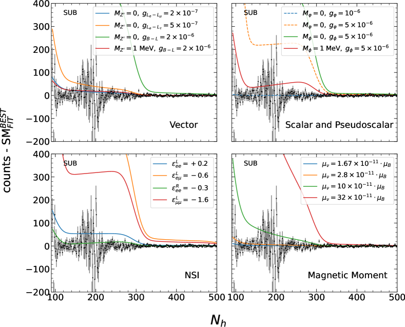
Figure 1: Difference between the number of events with respect to the SM expectation, as a function of $N_{h}$. For reference, the black dots are obtained for the data in the “subtracted” sample, where the error bars indicate statistical errors only. The coloured lines correspond to the predicted event rates (using the same exposure as that of the “subtracted” sample) for different BSM scenarios and parameter values, as indicated by the labels.

Our statistical analysis is based on the construction of a $\chi^{2}$ function based on the described experimental data, neutrino signal expectations and sources of backgrounds, as well as the effect of systematic uncertainties. We introduce the latter in terms of pulls $\xi_{r}$, which are then varied in order to minimize the $\chi^{2}$. The analysis includes a total of 27 pulls to account for the uncertainties in the background normalizations, detector performance, priors on the solar fluxes, and energy shifts (see Appendix B for details). Assuming a linear dependence of the event rates on the pulls, the minimization can be performed analytically provided the $\chi^{2}$ can be assumed to be Gaussian. Borexino collaboration bins their data in each sample using 858 bins, from $N_{h}=92$ to $N_{h}=950$. Such thin binning does not provide enough events in each bin to guarantee Gaussian statistics. So for convenience we rebin the data using coarser bins: the first 42 bins are rebinned in groups of 2, the next 210 bins in groups of 5, the next 260 bins in groups of 10 and the last 346 bins in groups of 50. This yields a total of 96 bins $k$ for each data sample, $s$, each of them having enough events to guarantee Gaussian statistics. Altogether the $\chi^{2}$ we employ reads:

$$\chi^{2}=\min_{\vec{\xi}}\Bigg{[}\sum_{s,k}\frac{\big{[}T_{s,k}(\vec{\xi})-O_{s,k}\big{]}^{2}}{O_{s,k}}+\sum_{r}(\xi^{\text{unc}}_{r})^{2}+\sum_{r,r^{\prime}}(\Sigma^{-1})_{rr^{\prime}}\,\xi_{r}^{\text{corr}}\,\xi_{r^{\prime}}^{\text{corr}}\Bigg{]}\,,$$ (22)

where $O_{s,k}$ is the observed number of events in bin $k$ of sample $s$ and $T_{s,k}$ is the corresponding predicted number of events in the presence of systematics

$$T_{s,k}(\vec{\xi})=T_{s,k}^{0}+\sum_{r}D_{s,k}^{r}\xi_{r}\,.$$ (23)

$D_{s,k}^{r}$ stands for the derivatives of the total event rates with respect to each pull, which are given in Appendix. B.

The last two terms in Eq. (22) are Gaussian bias factors which we include for those pulls for which some prior constraint should be accounted for. The first of those last terms correspond to pulls associated to uncorrelated (“unc”) uncertainties while the last one to correlated (“corr”) uncertainties. Here, $\Sigma$ stands for the covariance matrix used for the latter and it is given in Appendix B.

4 Results

This section summarizes our results from the spectral analysis of Borexino data, as outlined in Sec. 3, for the phenomenological scenarios defined in Sec. 2. We will first present our analysis for the magnetic moment scenario introduced in Sec. 4.1. As we will see, our results are in excellent agreement with those obtained in Ref. Borexino:2017fbd and therefore serve to validate our $\chi^{2}$ implementation (and, in particular, the implementation of systematic uncertainties) discussed in Sec. 3. We then proceed to the NSI scenario in Sec. 4.2, while the cases of light vector, scalar, and pseudoscalar mediators are shown in Secs. 4.3 and 4.4.

At this point it is worth stressing the technical challenges associated to the $\chi^{2}$ minimization procedure. The analysis, a priori, depends on 27 pulls, 6 standard oscillation parameters, plus a number of non-standard oscillation parameters (ranging from 2 to 6, depending on the particular scenario considered). In order to make the problem tractable from the computational point of view, we minimize analytically over the 27 pulls as outlined in the previous section, and we fix the oscillation parameters to the present best-fit values from Ref. Esteban:2020cvm ; nufit (we have checked that this has a negligible impact on the results). The exploration of the BSM parameter space is performed numerically, using the Diver software Martinez:2017lzg ; diver . We have also cross-checked that the resulting two-dimensional confidence regions agree with the result obtained using a simplex method algorithm.

Throughout this section, we will follow a frequentist approach in order to determine the allowed confidence regions for the parameters in each case. In other words, for a given BSM scenario characterized by a set of parameters $\vec{\omega}$, we define a $\Delta\chi^{2}$ function as:

$$\Delta\chi^{2}(\vec{\omega})=\chi^{2}(\vec{\omega})-\chi^{2}_{\text{min}}\,,$$ (24)

where $\chi^{2}_{\text{min}}$ refers to the global minimum of the $\chi^{2}$ function, found after minimization over all the model parameters $\vec{\omega}$. We stress that $\chi^{2}(\vec{\omega})$ corresponds to Eq. (22) where $T_{s,k}(\vec{\xi})$ is in fact $T_{s,k}(\vec{\omega},\,\vec{\xi})$ so the minimization over the pull parameters is performed for each given value of the model parameters. The allowed regions are then determined by the set of model parameters for which the $\Delta\chi^{2}$ lies below a certain level, as indicated in each case.

For reference let us mention that the analysis performed within the SM results into $\chi^{2}_{\text{min,SM}}=256.7$ for a total of 192 data points and 27 pull parameters.

4.1 Neutrino magnetic moment

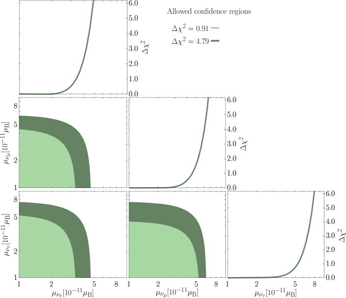
Figure 2: Results for the magnetic moment scenario, assuming three independent parameters (one for each of the SM neutrino flavours). Since the neutrino magnetic moment is positive definite, the cuts have been taken according to a one-sided $\chi^{2}$ distribution. In the central panels, we show the allowed confidence regions (at $1\sigma$ and $2\sigma$, for 2 d.o.f. using one-sided intervals) while in the right-most panels we show the profile of the $\Delta\chi^{2}$ for each of the parameters individually. In each panel, the results are obtained after minimization over the undisplayed parameters.

For the analysis with neutrino magnetic moment we find $\chi^{2}_{\mathrm{min,SM+\mu_{\nu}}}=256.5$. In other words, the data do not show a statistically significant preference for a non-vanishing magnetic moment, which allows to set constraints on the parameter space for this scenario. The corresponding results are summarized in Fig. 2, assuming three independent parameters for the $\nu_{e}$, $\nu_{\mu}$ and $\nu_{\tau}$ magnetic moments. In each panel, the $\Delta\chi^{2}$ is minimized over the undisplayed parameters. From the one-dimensional projections we can read the upper bounds at 90% CL (for 1 d.o.f., one-sided intervals, i.e., $\Delta\chi^{2}=1.64$)

$$\mu_{\nu_{e}}<3.7\times 10^{-11}\mu_{B}\,,\qquad\mu_{\nu_{\mu}}<5.0\times 10^{-11}\mu_{B}\,,\qquad\mu_{\nu_{\tau}}<5.9\times 10^{-11}\mu_{B}\,.$$ (25)

Our results are fully compatible with those in Ref. Borexino:2017fbd , considering the different choice of oscillation parameters assumed. If we assume that all flavours carry the same value of the neutrino magnetic moment then the dependence on the oscillation parameters cancels out and we obtain the following bound (at 90 % CL for 1 d.o.f., one-sided)

$$\mu_{\nu}<2.8\times 10^{-11}\mu_{B}\,.$$ (26)

This coincides precisely with the result obtained by the collaboration in Ref. Borexino:2017fbd , and serves as validation for the $\chi^{2}$ implementation and the choice of systematic uncertainties adopted in our analysis.

We notice that the Borexino bounds are stronger than those obtained by other experiments under the same flavour assumptions and CL. This is the case for the (over a decade old) experimental results of GEMMA Beda:2010hk ; Beda:2012zz ($\mu_{\nu}<2.9\times 10^{-11}\mu_{B}$) and TEXONO TEXONO:2006xds ($\mu_{\nu}<7.4\times 10^{-11}\mu_{B}$), as well as the bounds derived from recent results such as CONUS CONUS:2022qbb ($\mu_{\nu}<7.5\times 10^{-11}\mu_{B}$) and the combined analysis of Dresden-II and COHERENT Coloma:2022avw ($\mu_{\nu}<1.8\times 10^{-10}\mu_{B}$).

4.2 Non-Standard neutrino Interactions with electrons

Let us now discuss the case of NSI with electrons. In this scenario Borexino is sensitive to a total of 12 operators: 6 operators involving left-handed electrons (with coefficients $\varepsilon_{\alpha\beta}^{L}$) and 6 operators involving right-handed electrons (with coefficients $\varepsilon_{\alpha\beta}^{R}$), see Eq. (5). In all generality, a priori all operators should be considered at once in the analysis since all of them enter at the same order in the effective theory. However, including such a large number of parameters makes the problem numerically challenging, and the extraction of meaningful conclusions is also jeopardized by the multiple interference effects between the different coefficients. Thus, here we focus on four representative cases with a reduced set of operators, depending on the type of interaction that could lead to the terms in Eq. (5): (1) the axial vector case, where both left- and right-handed NSI operators are generated with equal strength but with opposite signs; (2) the purely vector case, where both types of operators are generated with equal strength and equal sign; and (3) the purely left- or purely right-handed cases, where only operators involving electrons of a given chirality are obtained. For each of these four benchmarks we include all operators in neutrino flavour space (all flavour-diagonal and off-diagonal operators) simultaneously in the analysis, allowing for interference and correlation effects among them.

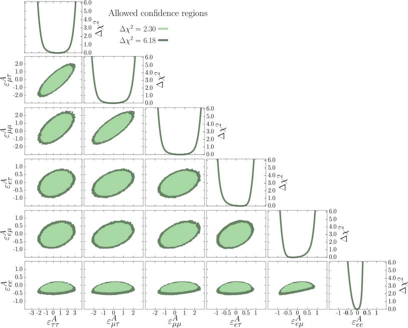
Figure 3: Results for axial NSI with electrons ($\varepsilon_{\alpha\beta}^{L}=-\varepsilon_{\alpha\beta}^{R}$). The central panels show the two-dimensional allowed confidence regions at $1\sigma$ and $2\sigma$ (for 2 d.o.f., using two-sided intervals $\Delta\chi^{2}=2.30$, $6.18$), while the remaining panels show the profile of the $\Delta\chi^{2}$ for each of the parameters individually. In each panel, the results are obtained after minimization over the parameters not shown.

We start discussing the axial NSI case. For axial NSI, the effect cancels out in the matter potential, rendering neutrino oscillations insensitive to the new interactions. However, Borexino can still constrain these operators since they affect the interaction cross section in the detector. First, we notice that even allowing all 6 axial NSI coefficients to vary freely we get $\chi^{2}_{\mathrm{min,SM+NSI^{A}}}=255.7$, which is only one unit lower that the SM. So we proceed to derive the bounds on the full parameter space.

The results are presented in Fig. 3 where we show one-dimensional and two-dimensional projections of $\Delta\chi^{2}_{\mathrm{SM+NSI^{A}}}$ after minimization over the parameters not shown in each panel. We notice that since the cross-section of flavour-conserving interactions receive contributions from both SM and BSM terms, which could lead to cancellations among them, the corresponding regions are generically larger than those involving only flavour-off-diagonal NSI, for which no SM term is present. From the figure we see that when all the parameters are included in the fit, Borexino is able to constrain NSI roughly only at the level of $|\varepsilon^{A}_{\alpha\alpha}|<\mathcal{O}(2)$ for flavour-diagonal interactions, and $|\varepsilon^{A}_{\alpha\neq\beta}|<\mathcal{O}(1)$ for the flavour-off-diagonal ones (see also Tab. 2). The only exception to this is the parameter $\varepsilon_{ee}^{A}$, for which tighter constraints are obtained, roughly at the level $|\varepsilon_{ee}^{A}|<\mathcal{O}(0.5)$ as it can be seen from the lowest row in the figure. The main reason behind this is that the $\varepsilon_{ee}^{A}$ parameter enters the effective cross section in Eq. (5) multiplied by $P_{ee}\sim 0.5$, while the remaining NSI parameters are multiplied either by $P_{e\mu},P_{e\tau}\sim 0.2-0.25$ or by off-diagonal elements in the density matrix (which are at most $\sim 0.2$).

Note also that the allowed regions for flavour-diagonal NSI are a bit asymmetric with respect to zero. In general, given the large parameter space it is difficult to identify a single reason for the specific shape of the allowed regions. Still, the origin of the asymmetry can be qualitatively understood if the generalized cross section matrix in Eq. (8) is written in terms of the axial and vector coefficients, defined (in analogy to Eq. (9)) as

$$C^{V}_{\alpha\beta} =C^{L}_{\alpha\beta}+C^{R}_{\alpha\beta}=c_{V\beta}\delta_{\alpha\beta}+\varepsilon^{V}_{\alpha\beta}\,,$$ (27)

$$C^{A}_{\alpha\beta} =C^{L}_{\alpha\beta}-C^{R}_{\alpha\beta}=c_{A\beta}\delta_{\alpha\beta}+\varepsilon^{A}_{\alpha\beta}\,.$$

In this case, the differential cross section for axial NSI, setting $\alpha=\beta$, depends on the following combination of parameters:

$$\frac{1}{2}\left(c_{V\alpha}^{2}+c_{A\alpha}^{2}\right)+c_{A\alpha}\varepsilon_{\alpha\alpha}^{A}+\frac{(\varepsilon^{A}_{\alpha\alpha})^{2}}{2}+\mathcal{O}(y)\,.$$ (28)

We notice that due to the interference between the SM and NSI parameters, a second SM-like solution appears in Eq. (28) with $\varepsilon^{A}_{\alpha\alpha}\simeq-2\,c_{A\alpha}$ (i.e., for which $C^{A}_{\alpha\alpha}=-c_{A,\alpha}$). It can actually be shown that for $\alpha=\mu$ and $\alpha=\tau$ such SM-like solution holds also after including the full $y$ dependence of the cross section and so it provides a fit of similar quality to the SM solution. When only one NSI parameter is considered at a time this leads to the two disconnected allowed ranges seen for $\varepsilon^{A}_{\mu\mu}$ and $\varepsilon^{A}_{\tau\tau}$ in Table 2. When all NSI parameters are included both allowed regions merge in a unique range which is asymmetric about zero. In the case of $\varepsilon^{A}_{ee}$, on the contrary, the $y$-dependent terms break such degeneracy and the second SM-like solution gets lifted.

From Eq. (28) we also see that for $\varepsilon^{A}_{\alpha\alpha}\simeq-c_{A\alpha}$ it is possible to reduce the cross section with respect to the SM case. This leads to a slightly better fit to the data (albeit mildly, at the level of $\Delta\chi^{2}=-1$ as mentioned above) and results into the preferred solution to be at $\varepsilon_{ee}^{A}\lesssim 0$ (since $c_{Ae}\sim 0.5$). Conversely, for $\varepsilon_{\mu\mu}^{A}$ and $\varepsilon_{\tau\tau}^{A}$ the fit shows a mild preference for positive values since $c_{A\mu}=c_{A\tau}\sim-0.5$.

Finally, it is worth stressing the impact of correlations in the fit, which are large for this scenario. For example, from the two-dimensional panels in Fig. 3 it is evident that there is a strong correlation between $\varepsilon^{A}_{\mu\tau}$, $\varepsilon^{A}_{\mu\mu}$, and $\varepsilon^{A}_{\tau\tau}$, which has a significant impact on the final limits obtained when all parameters are allowed to float freely in the fit. This is shown explicitly in Tab. 2, which compares the obtained bounds (at 90% CL) for the different NSI parameters in two different cases: turning on only one parameter at a time (“1 Parameter”), or including all operators simultaneously in the fit (“Marginalized”). As can be seen from the comparison between the two sets of results in this table, the impact due to correlations and degeneracies between different operators is significant and leads to considerably larger allowed regions if multiple NSI operators are included at once. For example, in the case of $\varepsilon_{\mu\mu}^{A}$, the 90% CL range is reduced by a factor of $\sim 8$ if the remaining NSI operators are set to zero.

	Allowed regions at 90% CL $(\Delta\chi^{2}=2.71)$
	Vector		Axial Vector
	1 Parameter	Marginalized	1 Parameter	Marginalized
$\varepsilon_{ee}$	$[-0.09,+0.14]$	$[-1.05,+0.17]$	$[-0.05,+0.10]$	$[-0.38,+0.24]$
$\varepsilon_{\mu\mu}$	$[-0.51,+0.35]$	$[-2.38,+1.54]$	$[-0.29,+0.19]\oplus[+0.68,+1.45]$	$[-1.47,+2.37]$
$\varepsilon_{\tau\tau}$	$[-0.66,+0.52]$	$[-2.85,+2.04]$	$[-0.40,+0.36]\oplus[+0.69,+1.44]$	$[-1.82,+2.81]$
$\varepsilon_{e\mu}$	$[-0.34,+0.61]$	$[-0.83,+0.84]$	$[-0.30,+0.43]$	$[-0.79,+0.76]$
$\varepsilon_{e\tau}$	$[-0.48,+0.47]$	$[-0.90,+0.85]$	$[-0.40,+0.38]$	$[-0.81,+0.78]$
$\varepsilon_{\mu\tau}$	$[-0.25,+0.36]$	$[-2.07,+2.06]$	$[-1.10,-0.75]\oplus[-0.13,+0.22]$	$[-1.95,+1.91]$

Table 2: 90% CL bounds (1 d.o.f., 2-sided) on the coefficients of NSI operators with electrons, for the vector ($\varepsilon^{V}$) and axial vector ($\varepsilon^{A}$) scenarios. Results are provided separately for two cases: when only one NSI operator is included at a time (“1 Parameter”) or when the remaining NSI coefficients are allowed to float freely in the fit (“Marginalized”).

Let us now turn to the analysis of vector NSI. In this case NSI affect the matter potential felt by neutrinos in propagation and a relevant question is how sensitive the analysis is to this effect, and whether the sensitivity to NSI is still dominated by the impact on the neutrino detection cross section. We have numerically checked that the results of the analysis are rather insensitive to NSI effects in propagation. This is partly so because in the energy window considered here the contribution from the higher-energy components (mainly $\mbox{}^{8}\text{B}$, but also pep neutrinos) to the event rates is subdominant, and moreover it is affected by relatively large backgrounds uncertainties. As a result we find that the impact of the matter potential on the fit is very limited and the sensitivity comes dominantly from NSI effects on the detection cross section. We also find that, even allowing all 6 vector NSI coefficients to vary freely in the analysis, $\chi^{2}_{\mathrm{min,SM+NSI^{V}}}-\chi^{2}_{\mathrm{min,SM}}$ is only $-0.2$.

Our allowed regions for vector NSI are presented in Fig. 4, where we see that the potential of Borexino to test NSI with electrons is again limited in this multi-parameter scenario: Borexino is only able to constrain NSI at the level of $|\varepsilon_{\alpha\alpha}^{V}|<\mathcal{O}(2-3)$ for flavour-diagonal interactions, and $|\varepsilon_{\alpha\beta}^{V}|<\mathcal{O}(1)$ for the off-diagonal parameters. Precise values for the allowed regions at 90% CL are given in Tab. 2.

The features describing the allowed regions in the two-dimensional projections of the $\Delta\chi^{2}$ are qualitatively similar to the results found for the axial case, albeit with some differences. In particular the regions for $\varepsilon_{\mu\mu}^{V}$ and $\varepsilon_{\tau\tau}^{V}$ are slightly more symmetric than the axial case. Again, this can be qualitatively understood if the cross section in Eq. (8) is rewritten in terms of the axial and vector couplings which results in Eq. (28) but replacing $c_{A\alpha}\leftrightarrow c_{V\alpha}$ and $\varepsilon^{A}_{\alpha\alpha}\leftrightarrow\varepsilon^{V}_{\alpha\alpha}$. Thus, a similar interference as in the axial case takes place here; however since $c_{V\mu}=c_{V\tau}\sim-0.04$ the quasi-degenerate SM-like solution lies closer to the SM so the region is more symmetric about zero.

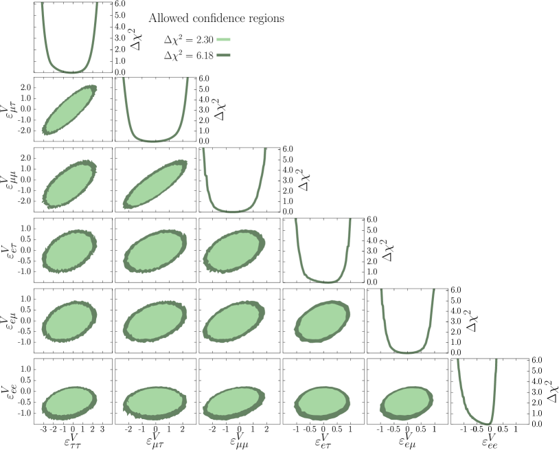
Figure 4: Same as Fig. 3, but for vector NSI with electrons ($\varepsilon_{\alpha\beta}^{L}=\varepsilon_{\alpha\beta}^{R}$).

For completeness, we also provide our results for NSI involving only left-handed and right-handed electrons in Tab. 3, where we again show the results obtained turning on only one operator at a time, and allowing all NSI operators simultaneously in the fit. We have numerically checked that, if only a single operator is included, we recover the results of the Borexino collaboration for both left-handed and right-handed NSI (Fig. 5 in Ref. Borexino:2019mhy ) with a very good accuracy. The only difference is the secondary minimum for $\varepsilon^{L}_{ee}\sim-1.3$ which is outside of the range of parameters explored in Ref. Borexino:2019mhy .

	Allowed regions at 90% CL $(\Delta\chi^{2}=2.71)$
	Left-handed		Right-handed
	1 Parameter	Marginalized	1 Parameter	Marginalized
$\varepsilon_{ee}$	$[-1.37,-1.29]\oplus[-0.03,+0.06]$	$[-1.48,+0.09]$	$[-0.23,+0.07]$	$[-0.53,+0.09]$
$\varepsilon_{\mu\mu}$	$[-0.20,+0.13]\oplus[+0.58,+0.81]$	$[-1.59,+2.21]$	$[-0.36,+0.37]$	$[-1.26,+0.77]$
$\varepsilon_{\tau\tau}$	$[-0.26,+0.26]\oplus[+0.45,+0.86]$	$[-2.00,+2.60]$	$[-0.58,+0.47]$	$[-1.45,+1.04]$
$\varepsilon_{e\mu}$	$[-0.17,+0.29]$	$[-0.78,+0.75]$	$[-0.21,+0.41]$	$[-0.43,+0.42]$
$\varepsilon_{e\tau}$	$[-0.26,+0.23]$	$[-0.81,+0.79]$	$[-0.35,+0.31]$	$[-0.39,+0.43]$
$\varepsilon_{\mu\tau}$	$[-0.62,-0.52]\oplus[-0.09,+0.14]$	$[-1.95,+1.91]$	$[-0.26,+0.23]$	$[-1.10,+1.03]$

Table 3: Constraints at 90% CL (for 1 d.o.f., 2-sided) on the coefficients of NSI operators involving only left-handed ($\varepsilon^{L}$) or right-handed ($\varepsilon^{R}$) electrons. Results are provided separately for two cases: when only one NSI operator is included at a time (“1 Parameter”) or when the remaining NSI coefficients are allowed to float freely in the fit (“Marginalized”).

4.3 Light vector mediators

The potential of Borexino to probe simplified models with light vector mediators has been demonstrated in the literature for the $B-L$ case Harnik:2012ni ; Bilmis:2015lja , and the bound has been later recast to other $U(1)^{\prime}$ models in Refs. Kaneta:2016uyt ; Bauer:2018onh . However, Refs. Harnik:2012ni ; Bilmis:2015lja date from 2012 and 2015 and therefore did not include Phase-II data. Furthermore, their bound was only approximate: it was derived requiring that the new physics contribution to the event rates should not exceed the SM expectation. Here we report our limits for simplified models, for our data analysis which includes full spectral information for the Phase II data and a careful implementation of systematic uncertainties.

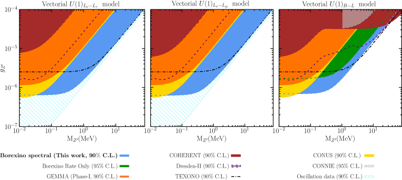
Figure 5: Bounds from our analysis of Borexino Phase II spectral data (at 90% CL for 1 d.o.f., using two-sided intervals, i.e., $\Delta\chi^{2}=2.71$) on the vector mediators associated to a new $U(1)^{\prime}$ symmetry, as indicated in the top label for each panel. Our results are compared to our derived bounds from GEMMA Beda:2010hk ; Coloma:2020gfv , TEXONO Deniz:2009mu ; Coloma:2020gfv , COHERENT COHERENT:2017ipa ; COHERENT:2020iec ; Coloma:2022avw , and Dresden-II reactor experiment Colaresi:2022obx ; Coloma:2022avw , as well as those derived from a global fit to oscillation data Coloma:2020gfv , all of them obtained with the same statistical criterion. We also show the bounds from CONNIE CONNIE:2019xid (95% CL) and CONUS CONUS:2021dwh (90% CL) which we have obtained applying an overall rescaling factor to their published bounds on a universally coupled vector (see text for details). For the $B-L$ model, the line labelled “Borexino Rate Only” shows the approximate bound derived (at 95% CL, 1 d.o.f., for one-sided intervals) in Ref. Bilmis:2015lja (see also Ref. Harnik:2012ni ).

Our results for vector mediators are presented in Fig. 5 for three anomaly-free models in which the vector couples to $B-L$, $L_{e}-L_{\mu}$, or $L_{e}-L_{\tau}$. As seen in the figure the results for the three models are very similar. This can be easily understood from Eqs. (3) and (16). In particular the dominant BSM contribution to the event rates arises from the interference term with the SM. So, the new physics will lead to a modification to the expected number of events that goes as

$$\Delta N_{\text{ev}}\propto\sum_{\beta}P_{e\beta}q_{Z^{\prime}}^{\nu_{\beta}}\,q_{Z^{\prime}}^{e}\,c_{V\beta}\sim P_{ee}\,q_{Z^{\prime}}^{\nu_{e}}\,q_{Z^{\prime}}^{e}\,c_{Ve}\,,$$ (29)

where we have removed the sum over neutrino flavours, as $c_{Ve}\sim 1\gg c_{V\mu(\tau)}\sim 0.04$ and $P_{ee}>P_{e\mu}\simeq P_{e\tau}$. Since for the three models considered $q_{Z^{\prime}}^{\nu_{e}}\,q_{Z^{\prime}}^{e}=1$, the derived bounds are about the same in the three cases.

For completeness, we also compare our Borexino results to previous bounds obtained in the literature. For the range of couplings considered here, the most relevant constraints come from CE$\nu$NS, neutrino scattering on electrons, and from neutrino oscillation data, while measurements of neutrino scattering on nuclei or electrons at high momentum transfer will be suppressed with the inverse of the momentum transfer squared (see, e.g., the discussion in Ref. Coloma:2017egw ). In principle, additional bounds are obtained from fixed-target experiments or colliders (for example, the $Z^{\prime}$ may be produced on-shell and decay to pairs of charged leptons). However, these bounds are a priori model-dependent: for example, if the new mediator decays predominantly to dark sector particles, some of them can be significantly relaxed. Thus, here we consider only those bounds from neutrino scattering and oscillation experiments, which always apply to the models considered (for a detailed compilation of constraints on light vector mediators we refer the interested reader to, e.g., Refs. Bauer:2018onh ; Coloma:2020gfv ). Specifically, we consider the following set of constraints:

• measurements of $\nu-e$ scattering at the reactor experiments GEMMA Beda:2010hk and TEXONO Deniz:2009mu , computed as in Ref. Coloma:2020gfv . Here we note that our analysis of GEMMA Phase-II shows a poor fit to the data (with or without BSM contributions). Naively including this dataset in the $\Delta\chi^{2}$ analysis results into strong bounds on the BSM models which, however, are not statistically robust. Thus, the results shown here for GEMMA correspond to Phase-I data alone, for which (under the SM hypothesis) we numerically find $\chi^{2}/n_{\text{d.o.f.}}\sim 26/39$, $n_{\text{d.o.f.}}$ being the number of bins.

• bounds from CE$\nu$NS measurements (on both CsI and Ar nuclei) at COHERENT COHERENT:2020iec ; COHERENT:2017ipa and at the Dresden-II reactor experiment Colaresi:2022obx , computed as in Ref. Coloma:2022avw (based on the analysis performed in Refs. Coloma:2019mbs ; Coloma:2020gfv ). Note that, although these experiments were designed to search for CE$\nu$NS (which dominates the sensitivity to $B-L$), they are also sensitive to $\nu$-e elastic scattering and therefore can be used to set constraints on the $L_{e}-L_{\mu}$ and $L_{e}-L_{\tau}$ models as well (see Ref. Coloma:2022avw for details). For concreteness, here we show the results for Dresden-II using the quenching factor labelled as “Fef” in Ref. Coloma:2022avw (qualitatively similar results are obtained for the “YBe” quenching factor).

• constraints derived from the impact of new vector mediators on the matter potential in neutrino oscillations. These were obtained from a global fit to oscillation data in Ref. Coloma:2020gfv . Note that these constraints only apply to flavoured $U(1)^{\prime}$ models (where the neutrino flavours have different charges under the new interaction) and therefore are absent in the $B-L$ case.

• bounds derived from searches for CE$\nu$NS at CONNIE CONNIE:2019xid , and from CE$\nu$NS and ES searches at CONUS CONUS:2021dwh . In both cases the bounds were reported for a vector mediator which couples universally to all SM fermions. The bounds obtained from ES searches coincide for the $B-L$ and the universal models, since $q_{Z^{\prime}}^{\nu_{e}}\,q_{Z^{\prime}}^{e}=1$ in the two cases. Regarding the bounds from CE$\nu$NS searches, the reported limits for the universal model are rescaled for the $B-L$ case, assuming an average momentum transfer. For CONNIE we quote the results obtained using the Lindhard quenching factor Lindhard . For CONUS, on the other hand, we take the results corresponding to a quenching factor for $k=0.16$ from Fig. 5 in Ref. CONUS:2021dwh . Notice that the excluded regions derived by CONUS in Ref. CONUS:2021dwh are given as 90% CL (see Ref. Rink:2022rsx for details), while for CONNIE CONNIE:2019xid the excluded regions are shown at 95% CL.

• for the $B-L$ model, we also show previous estimates of the Borexino constraint computed in Ref. Harnik:2012ni ; Bilmis:2015lja . These results are labelled as “Rate only”. As outlined above, these are obtained using data available prior to 2015, requiring that the new physics contribution to the total event rates in the energy region corresponding to the $\mbox{}^{7}\text{Be}$ line does not exceed the SM expectation (within reported uncertainties, which at the time were at the level of 8%). These limits were reported as one-sided constraints, at 95% CL with seemingly 1 d.o.f.

As can be seen, our results for Borexino qualitatively agree with the approximate bounds from Ref. Bilmis:2015lja , but lead to an improved constraint by a factor $\sim 60\%$ on the upper bound on $Z^{\prime}$ for very light mediators (and by about 30% on $g_{Z^{\prime}}/M_{Z^{\prime}}$ in the contact-interaction regime). Also, as seen in the figure, our analysis of Borexino Phase-II spectra leads to improvements on the bounds from scattering experiments in most of the parameter space, for the three models under consideration. On the other hand, the bounds from oscillation data prevail as the strongest constraints on the $L_{e}-L_{\mu}$ and $L_{e}-L_{\tau}$ models.

4.4 Light scalar and pseudoscalar mediators

Next let us discuss our results for a scalar (pseudoscalar) mediator coupled universally to the SM fermions, shown in the left (right) panel of Fig. 6. It is important to note that constraints from oscillation data do not apply to scalar (or pseudoscalar) mediators. For comparison, we also show the bounds derived from neutrino scattering measurements, computed following (or obtained from) the same references as in Sec. 4.3. Comparing the scattering constraints shown in Fig. 6 against the same bounds for vector mediators in Fig. 5, we find that, generically, the bounds imposed on the scalars (and more so for pseudoscalars) are somewhat weaker. This is expected because the dominant contribution for the vector interactions arise from the interference with the SM (which is quadratic on the new coupling constant) while the scalar (or pseudoscalar) contributions do not interfere with the SM and therefore the dependence on the new coupling constant is quartic. Furthermore as seen in Eqs. (12) and (14) the cross section in the scalar and pseudoscalar scenarios are suppressed as $T_{e}m_{e}/E_{\nu}^{2}$ and $T_{e}^{2}/E_{\nu}^{2}$, respectively, with respect to the vector-mediated scattering cross section in Eq. (16).

From the figure we see that our bounds from Borexino Phase II data improve over previous constraints from ES reactor experiments (GEMMA and TEXONO) in both panels. However, for scalar interactions (left panel) the strongest limits come from the Dresden-II reactor experiment, and Borexino is only able to give a comparable limit for very light mediator masses $M_{\phi}\sim 0.5~{}\text{MeV}$. This is so because for the universal model shown the scalar coupling to quarks would lead to additional contributions to CE$\nu$NS at the Dresden-II experiment (as well as for CONNIE and CONUS), which enhances their sensitivity in the high-mass region (see, e.g., Ref. Coloma:2022avw ). Conversely, in the pseudoscalar scenario our bounds from Borexino dominate for mediator masses $M_{\varphi}\lesssim 5~{}\text{MeV}$, with TEXONO being the only other experiment which provides a comparable result. This is so because pseudoscalars interactions couple to spin and therefore the corresponding CE$\nu$NS cross section can be safely neglected. Thus, the Dresden-II contour shown in the right panel has been obtained considering only the new physics contribution to ES (which would pass their signal selection cuts), leading to a worse constraint compared to the one obtained in the scalar case. Finally, note that while in principle it should also be possible to derive bounds on the pseudoscalar scenario using ES searches at CONUS, the collaboration did not study this scenario and therefore no limits from CONUS are available in this case. From the results for the scalar case we expect, however, that these would be weaker than the bound obtained from Borexino, since the cross section in the pseudoscalar case would be suppressed to that in the scalar scenario by an additional factor of $T_{e}/m_{e}$ (at CONUS, this factor can be estimated as $\mathcal{O}(\text{keV}/0.5~{}\text{MeV})\sim 2\times 10^{-3}$).

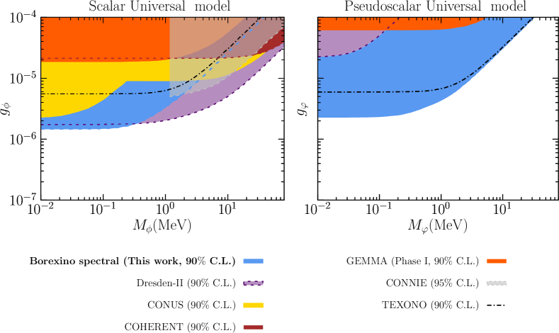
Figure 6: Bounds from our analysis of Borexino Phase-II spectral data on a scalar (left panel) and pseudoscalar (right panel) mediator (at 90% CL for 1 d.o.f., using two-sided intervals, i.e., $\Delta\chi^{2}=2.71$) which couples universally to all fermions in the SM. Our results are compared to our derived bounds from GEMMA Beda:2010hk ; Coloma:2020gfv , TEXONO Deniz:2009mu ; Coloma:2020gfv , COHERENT COHERENT:2017ipa ; COHERENT:2020iec ; Coloma:2022avw , and Dresden-II reactor experiment Colaresi:2022obx ; Coloma:2022avw , obtained using the same statistical criterion. For comparison we also show the bounds from CONNIE CONNIE:2019xid (95 %CL) and CONUS CONUS:2021dwh (90% CL).

5 Conclusions

In this work we have presented a detailed analysis of the spectral data of Borexino Phase II (corresponding to a total exposure of $1291.51~{}\text{days}\times 71.3~{}\text{tons}$) with the aim at exploiting its full potential to constrain BSM scenarios. Following closely the analysis of the collaboration, we have performed a detailed treatment of the background subtraction and careful accounting of all systematic uncertainties (particularly those associated with the energy reconstruction), including a total of 27 nuisance parameters in our fit. We have validated our constructed $\chi^{2}$ by performing a fit to the solar neutrino fluxes which accurately reproduces the results of Borexino Borexino:2017rsf , as shown in Figs. 8 and 9.

We have used our analysis to derive constraints on neutrino magnetic moments, NSI, and several simplified models with light scalar, pseudoscalar, and light vector mediators. In particular, for NSI we consider at the same time flavour off-diagonal as well as flavour-diagonal interactions. This brings the issue of the interplay between neutrino oscillations and interactions which do not conserve neutrino flavour, which has been often overlooked in the literature. We correctly account for those in terms of a density matrix (see Eq. (4)), which we provide for the specific case of NSI in Appendix A.

Our main results are presented in Sec. 4. For neutrino magnetic moments we have allowed different magnetic moments for the different neutrino flavours – albeit still imposing that they are flavour-diagonal – and obtained the bounds in Eq. (25). For flavour-independent magnetic moment we obtained the bound in Eq. (26). This is in perfect quantitative agreement with that obtained by the collaboration in Ref. Borexino:2017fbd and serves as an additional validation of our $\chi^{2}$ implementation.

Our analysis for NSI includes all operators with the same Lorentz structure: purely vector, axial vector, left-handed only, or right-handed only (6 parameters in each case, assumed to be real). Our results are shown in Figs. 3 and 4 as well as in Tables 2 and 3. We have numerically checked that, if only one NSI operator is included at a time, we recover the results in Ref. Borexino:2017fbd for the left-handed only and right-handed only scenarios, to a very good approximation. However, we find that when all couplings are allowed simultaneously, strong correlations appear and the bounds are substantially relaxed, as explicitly shown in Tables 2 and 3.

We have also derived new constraints for simplified models with new light vector, scalar, and pseudoscalar mediators which we show in Figs. 5 and 6. For mediator masses $M\lesssim 0.1$ MeV, the obtained experimental bound becomes independent of the mass of the mediator. Within this (effectively massless) regime, the bounds derived from Borexino data for the considered models read, at 90% CL (1 d.o.f., one-sided)

$$|g_{Z^{\prime}}^{B-L}| \leq 6.3\times 10^{-7}\,,$$ (30)

$$|g_{Z^{\prime}}^{L_{e}-L_{\mu}}| \leq 5.8\times 10^{-7}\,,$$

$$|g_{Z^{\prime}}^{L_{e}-L_{\tau}}| \leq 5.8\times 10^{-7}\,,$$

$$|g_{\phi}^{\text{univ}}| \leq 1.4\times 10^{-6}\,,$$

$$|g_{\varphi}^{\text{univ}}| \leq 2.2\times 10^{-6}\,.$$

Conversely, for sufficiently large mediator masses, the contact-interaction approximation is recovered and the event rates vary with a power of $(|g|/M)^{n}$ with $n=4$ for scalar mediators and with $n$ ranging between 2 and 4 for vector mediators. In this limit we get the following bounds at 90% CL (1 d.o.f., one-sided)

$$|g_{Z^{\prime}}^{B-L}|\,\big{/}M_{Z^{\prime}} \leq 1.4\times 10^{-6}~{}\text{MeV}^{-1}\quad\text{for} M_{Z^{\prime}} \gtrsim\text{few MeV}\,,$$ (31)

$$|g_{Z^{\prime}}^{L_{e}-L_{\mu}}|\,\big{/}M_{Z^{\prime}} \leq 1.2\times 10^{-6}~{}\text{MeV}^{-1}\quad\text{for} M_{Z^{\prime}} \gtrsim\text{few MeV}\,,$$

$$|g_{Z^{\prime}}^{L_{e}-L_{\tau}}|\,\big{/}M_{Z^{\prime}} \leq 1.2\times 10^{-6}~{}\text{MeV}^{-1}\quad\text{for} M_{Z^{\prime}} \gtrsim\text{few MeV}\,,$$

$$|g_{\phi}^{\text{univ}}|\,\big{/}M_{\phi} \leq 2.4\times 10^{-6}~{}\text{MeV}^{-1}\quad\text{for} M_{\phi} \gtrsim\text{MeV}\,,$$

$$|g_{\varphi}^{\text{univ}}|\,\big{/}M_{\varphi} \leq 2.5\times 10^{-6}~{}\text{MeV}^{-1}\quad\text{for} M_{\varphi} \gtrsim\text{MeV}\,.$$

Acknowledgements

This project has received funding/support from the European Union’s Horizon 2020 research and innovation program under the Marie Skłodowska-Curie grant agreement No 860881-HIDDeN, as well as from Grants PID2019-105614GB-C21, PID2019-110058GB-C21, PID2019-108892RB-I00, PID2020-113644GB-I00, “Unit of Excellence Maria de Maeztu 2020-2023" award to the ICC-UB CEX2019-000918-M, and Grant IFT Centro de Excelencia Severo Ochoa No CEX2020-001007-S, funded by MCIN/AEI/10.13039/501100011033, and by the “Generalitat Valenciana” grant PROMETEO/2019/087, and by AGAUR (Generalitat de Catalunya) grant 2017-SGR-929. MCGG is also supported by USA-NSF grant PHY-1915093. PC is also supported by Grant RYC2018-024240-I funded by MCIN/AEI/ 10.13039/501100011033 and by “ESF Investing in your future”. SU acknowledges support from Generalitat Valenciana through the plan GenT program (CIDEGENT/2018/019).

Appendix A Oscillations with non-standard interactions

In this appendix summarize the quantities relevant for the analysis of solar neutrino experiments. We will assume that only the first two mass eigenstates are dynamical, while the third is taken to be infinitely heavy. Since physical quantities have to be independent of the parameterization of the mixing matrix, we choose a parameterization that makes analytical expressions particularly simple. We start from the Hamiltonian in the flavour basis:

$$H=U\Delta U^{\dagger}+V\,,$$ (32)

where $\Delta=\operatorname{diag}(0,\Delta m^{2}_{21},\Delta m^{2}_{31})/2E$ and $V=\sqrt{2}G_{F}\big{[}N_{e}(x)\operatorname{diag}(1,0,0)+\sum_{f}N_{f}(x)\varepsilon_{\alpha\beta}^{f}\big{]}$. It is convenient to write $U=OU_{12}$, where $O=R_{23}R_{13}$ is real while $U_{12}$ is a complex rotation by angle $\theta_{12}$ and phase $\delta_{\text{CP}}$. Then we can write:

$$H=O\tilde{H}O^{\dagger}\qquad\text{with}\qquad\tilde{H}=U_{12}\Delta U_{12}^{\dagger}+O^{\dagger}VO\,.$$ (33)

In order to further simplify the analysis, let us now assume that all the mass-squared differences involving the “heavy” states $\nu_{3}$ can be considered as infinite: $\Delta m^{2}_{3l}\to\infty$ for $l=1,2$. In leading order, the matrix $\tilde{H}$ takes the effective block-diagonal form:

$$\tilde{H}\approx\begin{pmatrix}H^{(2)}&\boldsymbol{0}\\ \boldsymbol{0}&\Delta_{33}\end{pmatrix}$$ (34)

where $H^{(2)}$ is the $2\times 2$ sub-matrix of $\tilde{H}$ corresponding to the first and second neutrino states. Consequently, the evolution matrix is:

$$\tilde{S}\approx\begin{pmatrix}S^{(2)}&\boldsymbol{0}\\ \boldsymbol{0}&e^{-i\Delta_{33}L}\end{pmatrix}\quad\text{with}\quad S^{(2)}=\operatorname{Evol}\big{[}H^{(2)}\big{]}\quad\text{and}\quad S=O\tilde{S}O^{\dagger}\,.$$ (35)

We are interested only in the elements $S_{\alpha e}$. From the definition of $O$ we see that $O_{e2}=0$. Taking into account the block-diagonal form of $\tilde{S}$, we obtain:

$$S_{\alpha e}=O_{e1}\left(O_{\alpha 1}S_{11}^{(2)}+O_{\alpha 2}S_{21}^{(2)}\right)+O_{\alpha 3}O_{e3}e^{-i\Delta_{33}L}\,.$$ (36)

In order to derive explicit expression, let us begin writing $H^{(2)}=H_{\text{vac}}^{\text{(2)}}+H_{\text{mat}}^{\text{(2)}}$ with:

$$H_{\text{vac}}^{\text{(2)}} =\frac{\Delta m^{2}_{21}}{4E_{\nu}}\begin{pmatrix}-\cos 2\theta_{12}\,\hphantom{e^{-i\delta_{\text{CP}}}}&~{}\sin 2\theta_{12}\,e^{i\delta_{\text{CP}}}\\ \hphantom{-}\sin 2\theta_{12}\,e^{-i\delta_{\text{CP}}}&~{}\cos 2\theta_{12}\,\hphantom{e^{i\delta_{\text{CP}}}}\end{pmatrix},$$ (37)

$$H_{\text{mat}}^{\text{(2)}} =\sqrt{2}G_{F}\left[N_{e}(x)\begin{pmatrix}c_{13}^{2}&0\\ 0&0\end{pmatrix}+\sum_{f}N_{f}(x)\begin{pmatrix}-\varepsilon_{D}^{f\hphantom{*}}&\varepsilon_{N}^{f}\\ \hphantom{+}\varepsilon_{N}^{f*}&\varepsilon_{D}^{f}\end{pmatrix}\right],$$ (38)

The coefficients $\varepsilon_{D}^{f}$ and $\varepsilon_{N}^{f}$ are related to the original parameters $\varepsilon_{\alpha\beta}^{f}$ by the relations:

$$\begin{split}\varepsilon_{D}^{f}&=c_{13}s_{13}\,\mathop{\mathrm{Re}}\big{(}s_{23}\,\varepsilon_{e\mu}^{f}+c_{23}\,\varepsilon_{e\tau}^{f}\big{)}-\big{(}1+s_{13}^{2}\big{)}\,c_{23}s_{23}\,\mathop{\mathrm{Re}}\big{(}\varepsilon_{\mu\tau}^{f}\big{)}\\ &\hphantom{={}}-\frac{c_{13}^{2}}{2}\big{(}\varepsilon_{ee}^{f}-\varepsilon_{\mu\mu}^{f}\big{)}+\frac{s_{23}^{2}-s_{13}^{2}c_{23}^{2}}{2}\big{(}\varepsilon_{\tau\tau}^{f}-\varepsilon_{\mu\mu}^{f}\big{)}\,,\end{split}$$ (39)

$$\varepsilon_{N}^{f} =c_{13}\big{(}c_{23}\,\varepsilon_{e\mu}^{f}-s_{23}\,\varepsilon_{e\tau}^{f}\big{)}+s_{13}\left[s_{23}^{2}\,\varepsilon_{\mu\tau}^{f}-c_{23}^{2}\,\varepsilon_{\mu\tau}^{f*}+c_{23}s_{23}\big{(}\varepsilon_{\tau\tau}^{f}-\varepsilon_{\mu\mu}^{f}\big{)}\right].$$ (40)

Finally, it is convenient to introduce the following effective quantities:

$$P_{\text{osc}}^{(2)}\equiv|S_{21}^{(2)}|^{2}\,,\qquad P_{\text{int}}^{(2)}\equiv\mathop{\mathrm{Re}}\big{(}S_{11}^{(2)}S_{21}^{(2)*}\big{)}\,,\qquad P_{\text{ext}}^{(2)}\equiv\mathop{\mathrm{Im}}\big{(}S_{11}^{(2)}S_{21}^{(2)*}\big{)}\,,$$ (41)

and to provide the full matrix expression for $O$:

$$O=\begin{pmatrix}c_{13}&0&s_{13}\\ -s_{13}s_{23}&c_{23}&c_{13}s_{23}\\ -s_{13}c_{23}&-s_{23}&c_{13}c_{23}\end{pmatrix}.$$ (42)

A.1 Neutrino conversion probabilities

Let us begin from the flavour conversion probabilities, $P_{\alpha e}=|S_{\alpha e}|^{2}$. From Eq. (36) it is straightforward to derive:

$$P_{\alpha e}=|O_{e1}|^{2}\left[|O_{\alpha 1}|^{2}|S_{11}^{(2)}|^{2}+|O_{\alpha 2}|^{2}|S_{21}^{(2)}|^{2}+2\mathop{\mathrm{Re}}\big{(}O_{\alpha 1}O_{\alpha 2}S_{11}^{(2)}S_{21}^{(2)*}\big{)}\right]+|O_{\alpha 3}|^{2}|O_{e3}|^{2}$$ (43)

where we have used the fact that the term containing a factor $e^{-i\Delta_{33}L}$ oscillates very fast, and therefore vanish once the finite energy resolution of the detector is taken into account. This expression can be generically written as:

$$P_{\alpha e}=c_{13}^{2}\big{[}A_{\alpha}P_{\text{osc}}^{(2)}+B_{\alpha}P_{\text{int}}^{(2)}\big{]}+D_{\alpha}$$ (44)

with

$$A_{\alpha}\equiv|O_{\alpha 2}|^{2}-|O_{\alpha 1}|^{2}\,,\qquad B_{\alpha}\equiv 2\,O_{\alpha 1}O_{\alpha 2}\,,\qquad D_{\alpha}\equiv\sum_{i=\text{all}}|O_{\alpha i}|^{2}|O_{ei}|^{2}\,.$$ (45)

From Eq. (42) we get:

$$A_{\alpha}$$

(46)

A.2 Neutrino density matrix

Let us now turn to the expression for the density matrix, $\rho_{\alpha\beta}^{(e)}=S_{\alpha e}S_{\beta e}^{*}$. Again, from Eq. (36) we get:

$$\rho_{\alpha\beta}^{(e)}=|O_{e1}|^{2}\Big{[}O_{\alpha 1}O_{\beta 1}|S_{11}^{(2)}|^{2}+O_{\alpha 2}O_{\beta 2}|S_{21}^{(2)}|^{2}+O_{\alpha 1}O_{\beta 2}S_{11}^{(2)}S_{21}^{(2)*}+O_{\alpha 2}O_{\beta 1}S_{11}^{(2)*}S_{21}^{(2)}\Big{]}\\ +O_{\alpha 3}O_{\beta 3}|O_{e3}|^{2}$$ (47)

in full analogy with Eq. (43). As before, this expression can generically be written as:

$$\rho_{\alpha\beta}^{(e)}=c_{13}^{2}\big{[}A_{\alpha\beta}P_{\text{osc}}^{(2)}+B_{\alpha\beta}P_{\text{int}}^{(2)}+iC_{\alpha\beta}P_{\text{ext}}^{(2)}\big{]}+D_{\alpha\beta}$$ (48)

with

$$A_{\alpha\beta} \equiv O_{\alpha 2}O_{\beta 2}-O_{\alpha 1}O_{\beta 1}\,, \qquad B_{\alpha\beta} \equiv O_{\alpha 1}O_{\beta 2}+O_{\alpha 2}O_{\beta 1}\,,$$ (49)

$$C_{\alpha\beta} \equiv O_{\alpha 1}O_{\beta 2}-O_{\alpha 2}O_{\beta 1}\,, \qquad D_{\alpha\beta} \equiv\sum_{i=\text{all}}O_{\alpha i}O_{\beta i}|O_{ei}|^{2}\,.$$

General expressions for the $A_{\alpha\beta}$, $B_{\alpha\beta}$, $C_{\alpha\beta}$ and $D_{\alpha\beta}$ matrices can be easily obtained.

Appendix B Details of the Borexino analysis

B.1 Energy Calibration

As mentioned in the text, we perform the fit to Borexino data in terms of the observed number of hits $N_{h}$ as estimator of the recoil energy of the electron scattered by the incoming neutrinos. Energy resolution is included as the Gaussian function in Eq. (20) which gives the probability that an event with electron recoil energy $T_{e}$ yields an observed number of hits $N_{h}$ in terms of two parameters, the mean value of $N_{h}$ for a given $T_{e}$, $\bar{N}_{h}(T_{e})$, and the width of the probability distribution $\sigma_{h}(T_{e})$. To determine these two parameters as functions of $T_{e}$ we proceed in in two steps.

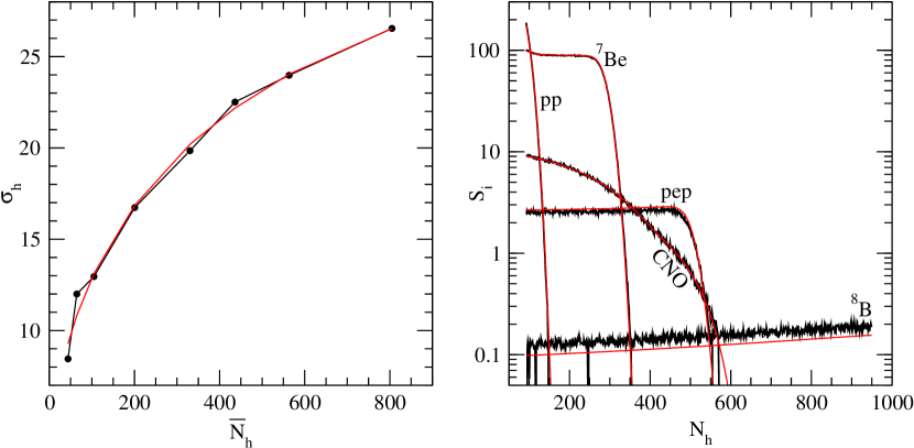
Figure 7: Left: our choice of the energy resolution function, based on the relation between $\sigma_{h}$ and $\bar{N}_{h}$ inferred from the upper panel of Fig. 22 of Ref. Borexino:2017rsf . Right: our reconstruction of solar spectra after the optimization of the energy scale function.

First we obtain the dependence of $\sigma_{h}\left(\bar{N}_{h}\right)$ from the calibration results of Borexino published in Ref. Borexino:2017mly . Concretely, by fitting the data from the upper panel of Fig. 22 of the published version (Fig. 21 in the arXiv version) with Gaussian distributions, we derive a relation between $\bar{N}_{h}$ and $\sigma_{h}$, which is depicted in the left panel of Fig. 7 and which reads:

$$\sigma_{h}(\bar{N}_{h})=1.21974+1.31394\sqrt{\bar{N}_{h}}-0.0148585\bar{N}_{h}\,.$$ (50)

The calibration results were obtained with a $\gamma$-ray source. And the basic assumption is that Eq. (50) holds equally for electrons.

Second we introduce that resolution function, which is now a function of $\bar{N}_{h}$, in our evaluation of the expected event rates for the different solar fluxes and infer the dependence of $\bar{N}_{h}(T_{e})$ which best reproduces the solar spectra depicted by Borexino in Fig. 7 of Ref. Borexino:2017rsf . We assume a 3rd-degree polynomial relation and find the best agreement to be with

$$\bar{N}_{h}(T_{e})=-8.065244+493.2560\bigg{[}\frac{T_{e}}{\text{MeV}}\bigg{]}-64.09629\bigg{[}\frac{T_{e}}{\text{MeV}}\bigg{]}^{2}+4.146102\bigg{[}\frac{T_{e}}{\text{MeV}}\bigg{]}^{3}.$$ (51)

The agreement we find between the Borexino solar spectra and our own calculations can be seen in the right panel of Fig. 7.

B.2 Implementation of systematics uncertainties, and assumed priors

In our analysis we introduce a total of 22 uncorrelated pulls to include background normalization uncertainties, signal and background systematic uncertainties related to the detector performance, and energy shift uncertainties. In addition 5 correlated pulls are used to introduce the SSM priors on the solar flux components. Here we discuss the implementation these different types of uncertainties separately.

Background normalizations

We consider 9 different background sources. Seven correspond to radioactive isotopes contaminating the scintillator, $\mbox{}^{14}\text{C}$, $\mbox{}^{11}\text{C}$, $\mbox{}^{10}\text{C}$, $\mbox{}^{210}\text{Po}$, $\mbox{}^{210}\text{Bi}$, $\mbox{}^{85}\text{Kr}$, and $\mbox{}^{6}\text{He}$. Two additional additional backgrounds are due to pile-up of uncorrelated events, and residual external backgrounds (we refer in what follows to this last one as “ext”).

We read the 18 (9 for each data sample) spectra and best fit normalization for these backgrounds from the results in Fig. 7 of Ref. Borexino:2017rsf . Following the procedure described in that reference we allow their normalization to vary in the fit. We do so by introducing a set of 11 independent pulls of which 7 corresponding to the normalizations of $\mbox{}^{14}\text{C}$, $\mbox{}^{10}\text{C}$, $\mbox{}^{210}\text{Bi}$, $\mbox{}^{85}\text{Kr}$, $\mbox{}^{6}\text{He}$, pile-up and ext which are assumed to be the same for both data samples, and 4 to the normalization of $\mbox{}^{11}\text{C}$, $\mbox{}^{210}\text{Po}$ which are left to be different in the tagged and the subtracted samples. The normalizations corresponding to $\mbox{}^{10}\text{C}$, $\mbox{}^{210}\text{Bi}$, $\mbox{}^{6}\text{He}$, $\mbox{}^{11}\text{C}_{\text{tag}}$, $\mbox{}^{210}\text{Po}_{\text{tag}}$, and $\mbox{}^{210}\text{Po}_{\text{sub}}$ are left unconstrained and therefore for them no bias factor is included in the $\chi^{2}$. For the other normalizations we include priors following the information provided in Ref. Borexino:2017rsf .

The effect of these 11 pulls is included as described in Eq. (23) in terms of the corresponding derivatives

$$D_{s,i}^{c}=\sigma_{c}\,B_{s,i}^{c}\quad\text{for}\quad c\in\{\mbox{}^{14}\text{C},\mbox{}^{11}\text{C}_{\text{sub}},\mbox{}^{85}\text{Kr},\text{pile-up},\text{ext}\}$$ (52)

with

$$\sigma_{\text{C14}}=0.05,\quad\sigma_{\text{C11,sub}}=0.0357,\quad\sigma_{\text{Kr}}=0.0368,\quad\sigma_{\text{ext}}=0.0484,\quad\sigma_{\text{pile-up}}=0.02,$$ (53)

and

$$D_{s,i}^{c}=B_{s,i}^{c}\quad\text{for}\quad c\in\{\mbox{}^{11}\text{C}_{\text{tag}},\mbox{}^{10}\text{C},\mbox{}^{210}\text{Po}_{\text{tag}},\mbox{}^{210}\text{Po}_{\text{sub}},\mbox{}^{210}\text{Bi},\mbox{}^{6}\text{He}\}$$ (54)

where for convenience we label the $r=1,\dots,11$ pulls by a label $c$ which specifies the background component they normalize.

Uncorrelated detector related signal and background uncertainties

We introduce eight pulls to parametrize the systematic uncertainties related to detector performance and background modelling. Their corresponding derivatives are:

$$D_{s,i}^{r}=\sum_{f}\sigma_{f}^{r}\,S_{s,i}^{f}+\sum_{c}\sigma_{c}^{r}\,B_{s,i}^{c}\,,$$ (55)

where $\sigma_{f}^{r}$ and $\sigma_{c}^{r}$ denote the assumed uncertainties for their effect each signal ($S_{s,i}^{f}$) and background ($B_{s,i}^{c}$) component, respectively. The values used in our fit are provided in the upper and lower sections of Tab. 4, respectively.

	$\xi_{1}$	$\xi_{2}$	$\xi_{3}$	$\xi_{4}$	$\xi_{5}$	$\xi_{6}$	$\xi_{7}$	$\xi_{8}$
pp	1.2%	2.5%	1.5%	3.0%	2.5%	2.2%	0.5%	0.853%
Be	0.2%	0.1%	—	0.1%	0.6%	0.2%	0.5%	0.853%
pep	4.0%	2.4%	—	1.0%	4.8%	1.6%	0.5%	0.853%
CNO	4.0%	2.4%	—	1.0%	4.8%	1.6%	0.5%	0.853%
B	—	—	—	—	—	—	0.5%	0.853%
C14	—	2.5%	—	—	—	—	—	0.853%
pile-up	—	—	1.5%	—	—	—	—	0.853%
C11	—	—	—	—	—	—	—	0.853%
C10	—	—	—	—	—	—	—	0.853%
Po	—	—	—	—	—	—	—	0.853%
Bi	—	—	—	—	—	—	—	0.853%
Kr	—	—	—	—	—	—	—	0.853%
He	—	—	—	—	—	—	—	0.853%
Ext	—	—	—	—	—	—	—	0.853%

Table 4: Prior uncertainties assumed for each signal component $\sigma_{f}^{r}$ (upper part of the table) and for each background component $\sigma_{c,\text{sub}}^{r}=\sigma_{c,\text{tag}}^{r}$ (lower part), for the eight nuisance parameters used to account for systematic uncertainties in the fit. Here, $\xi_{1}-\xi_{6}$ correspond to the six first sources of systematic uncertainties listed in Tab. IV of Ref. Borexino:2017rsf where they only show their effect on the determination of the solar fluxes in the Borexino fit. $\xi_{2}$ corresponds to the choice of energy estimator which we find to be also to be relevant for the determination of the steeply falling $\mbox{}^{14}\text{C}$ background. $\xi_{3}$ corresponds to the pile-up modelling so we assign similar uncertainties for the effect of that pull on the pile-up background. $\xi_{8}$ corresponds to the combined uncertainty on the live time, scintillator density and fiducial volume uncertainty from the same table which we assume affect all signals and backgrounds. $\xi_{7}$ refers to an overall normalization error of the elastic scattering cross-section Bahcall:1995mm (which only affects the signal).

Energy shift uncertainties

In addition to the systematic uncertainties describe above we also introduce a set of pulls to account for possible systematic shifts in the energy spectra for the different backgrounds that we have read from Fig. 7 of Ref. Borexino:2017rsf . We came out to the need of this additional pulls by noticing that the Borexino data shown in that figure can be extracted in two different ways: directly from the upper panels in that figure, or using the residuals provided in the lower panels, and assuming that these have been obtained with respect to the best-fit lines shown in the upper panels. The results obtained in these two ways should be equivalent but we found that this was not the case.

From further inspection of the data obtained in these two ways, it was clear that they were partially shifted in energy with respect to one another. This is most evident for the signal and background components with steepest energy dependence which happen to occur in the lowest part of the spectrum where the statistics is higher, and therefore the effect in the quality of the fit most relevant. We find that the introduction of an add-hoc energy shift of about $0.25N_{h}$ is able to reduce significantly the discrepancy observed between the two data sets, reconciling the two results. Thus, in our fit we use the data extracted from the upper panels in their Fig. 7, but we include additional pull terms in order to correct for a possible shift in energy. Since such energy shift has the largest impact in the low-energy part of the spectrum (and, most notably, on the pp solar neutrinos), we introduce three pulls: one for the $\mbox{}^{14}\text{C}$ and pile-up backgrounds, another one for the $\mbox{}^{11}\text{C}$ background, and a third pull for the $\mbox{}^{210}\text{Po}$ background.

Their corresponding derivatives are numerically computed as

$$D_{s,i}^{h}=\frac{B_{s,i+1}^{h}-B_{s,i-1}^{h}}{2}\quad\text{for}\quad h\in\{\mbox{}^{14}\text{C}+\text{pile-up},\mbox{}^{11}\text{C},\mbox{}^{210}\text{Po}\}\,,$$ (56)

for the original binning $i=1,\ldots 858$. So that for our coarse binning they are

$$D_{s,k}^{h}=\sum_{i}D_{s,i}^{h}\quad\text{for $i$ such that}\quad N_{h}^{i}\in[N_{h,\text{min}}^{k},N_{h,\text{max}}^{k}]\,,$$ (57)

for $k=1,\dots,96$.

Correlated uncertainties on the solar fluxes

The goal of our analysis of Borexino data is constraining the BSM scenarios presented in Sec. 2. For that we assume the solar fluxes to be as given by the Standard Solar Model (SSM). Technically this is enforced by introducing five pulls for the normalization of the five flux components of the solar neutrino signal subject to the priors of the SSM in both their central values, uncertainties and correlations. We introduce those by means of a covariance matrix $\Sigma$ which we obtain from Ref. Vinyoles:2016djt ; aldoweb . In our calculations, we use the high-metallicity (HZ) solar model for simplicity. So in this case the corresponding derivatives are simply:

$$D_{s,i}^{f}=S_{s,i}^{f}\quad\text{for}\quad f\in\{\text{pp},\mbox{}^{7}\text{Be},\text{pep},\text{CNO},\mbox{}^{8}\text{B}\}$$ (58)

B.3 Comparison to the results of the collaboration

As a first validation of our constructed $\chi^{2}$ function we perform an analysis which intends to reproduce the fit of the collaboration in Ref. Borexino:2017rsf to determine the solar neutrino fluxes. So we make a fit in which we do not include the covariance matrix for the solar fluxes previously described. Instead we leave the solar pp, $\mbox{}^{7}\text{Be}$ and pep neutrino signal fluxes completely free. We do introduce two priors for the CNO and $\mbox{}^{8}\text{B}$ the SSM (for concreteness we chose the high metallicity version of the model) as Borexino does. In the analysis we fit all background normalizations with the priors described above, and include the eight pulls for the uncorrelated systematics and the the three pulls for the energy shift. The result for our best fitted spectra (this is, our version of Fig. 7 in Ref. Borexino:2017rsf ) is shown in Fig. 8. The dependence of our $\Delta\chi^{2}$ on the normalization of the solar fluxes and the dominant backgrounds is shown in Fig. 9. The flux normalizations in the figure are normalized to the best fit values obtained by Borexino collaboration, hence a value of “1” means perfect agreement between our best fit fluxes and those of the collaboration. For comparison we also show for the solar fluxes as grey lines the inferred $\Delta\chi^{2}$ from the results quoted by the collaboration in Table II of Ref. Borexino:2017rsf (assuming it is approximately Gaussian). The figures show that our constructed event rates, the best-fit normalization of all signal and background components, and the precision in the determination of the solar fluxes reproduce with very good accuracy those of the fit performed by the collaboration. Ref. Borexino:2017rsf does not give enough information for a quantitative comparison of the $\Delta\chi^{2}$ for background normalizations, but we find that the precision we obtain for those is in good qualitative agreement with the results in Table III and Fig. 5 of Ref. Borexino:2017rsf .

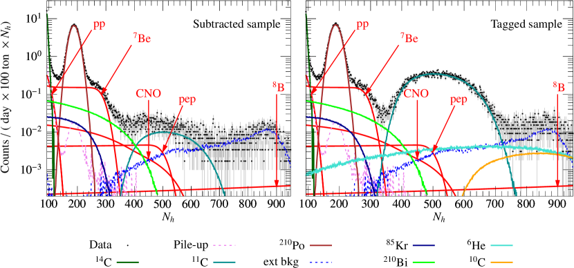
Figure 8: Spectrum for the best-fit normalizations of the different components obtained from our fit to the Borexino Phase II data for TFC-subtracted (left) and TFC-tagged events.

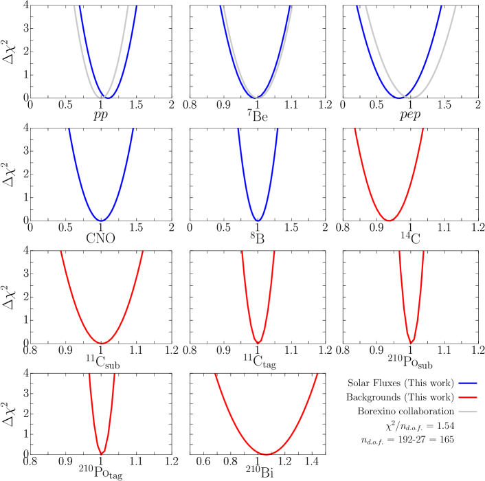
Figure 9: Dependence of $\Delta\chi^{2}$ of fit to the Borexino phase-II spectra on the normalization of the solar fluxes and the dominant backgrounds (normalized to the corresponding best fit normalizations of the fit of the Borexino collaboration in Ref. Borexino:2017rsf ). For comparison we show as light blue curves the corresponding results of the determination of solar fluxes in Ref. Borexino:2017rsf ) (see text for details).

References

- (1) CHARM-II collaboration, P. Vilain et al., Measurement of differential cross-sections for muon-neutrino electron scattering, Phys. Lett. B 302 (1993) 351–355.
- (2) R. C. Allen et al., Study of electron-neutrino electron elastic scattering at LAMPF, Phys. Rev. D 47 (1993) 11–28.
- (3) LSND collaboration, L. B. Auerbach et al., Measurement of electron - neutrino - electron elastic scattering, Phys. Rev. D 63 (2001) 112001, [hep-ex/0101039].
- (4) F. Reines, H. S. Gurr and H. W. Sobel, Detection of anti-electron-neutrino e Scattering, Phys. Rev. Lett. 37 (1976) 315–318.
- (5) G. S. Vidyakin, V. N. Vyrodov, I. I. Gurevich, Y. V. Kozlov, V. P. Martemyanov, S. V. Sukhotin et al., Limitations on the magnetic moment and charge radius of the electron-anti-neutrino, JETP Lett. 55 (1992) 206–210.
- (6) A. I. Derbin, A. V. Chernyi, L. A. Popeko, V. N. Muratova, G. A. Shishkina and S. I. Bakhlanov, Experiment on anti-neutrino scattering by electrons at a reactor of the Rovno nuclear power plant, JETP Lett. 57 (1993) 768–772.
- (7) MUNU collaboration, Z. Daraktchieva et al., Final results on the neutrino magnetic moment from the MUNU experiment, Phys. Lett. B 615 (2005) 153–159, [hep-ex/0502037].
- (8) TEXONO collaboration, H. T. Wong et al., A Search of Neutrino Magnetic Moments with a High-Purity Germanium Detector at the Kuo-Sheng Nuclear Power Station, Phys. Rev. D 75 (2007) 012001, [hep-ex/0605006].
- (9) A. G. Beda, V. B. Brudanin, V. G. Egorov, D. V. Medvedev, V. S. Pogosov, M. V. Shirchenko et al., The results of search for the neutrino magnetic moment in GEMMA experiment, Adv. High Energy Phys. 2012 (2012) 350150.
- (10) A. G. Beda, V. B. Brudanin, V. G. Egorov, D. V. Medvedev, V. S. Pogosov, E. A. Shevchik et al., Gemma experiment: The results of neutrino magnetic moment search, Phys. Part. Nucl. Lett. 10 (2013) 139–143.
- (11) CONUS collaboration, H. Bonet et al., Constraints on Elastic Neutrino Nucleus Scattering in the Fully Coherent Regime from the CONUS Experiment, Phys. Rev. Lett. 126 (2021) 041804, [2011.00210].
- (12) T. Rink, Investigating Neutrino Physics within and beyond the Standard Model using CONUS Experimental Data. PhD thesis, U. Heidelberg (main), 2022. 10.11588/heidok.00031274.
- (13) CONNIE collaboration, A. Aguilar-Arevalo et al., Search for light mediators in the low-energy data of the CONNIE reactor neutrino experiment, JHEP 04 (2020) 054, [1910.04951].
- (14) J. Colaresi, J. I. Collar, T. W. Hossbach, C. M. Lewis and K. M. Yocum, Suggestive evidence for Coherent Elastic Neutrino-Nucleus Scattering from reactor antineutrinos, 2202.09672.
- (15) P. Coloma, I. Esteban, M. C. Gonzalez-Garcia, L. Larizgoitia, F. Monrabal and S. Palomares-Ruiz, Bounds on new physics with data of the Dresden-II reactor experiment and COHERENT, 2202.10829.
- (16) COHERENT collaboration, D. Akimov et al., Observation of Coherent Elastic Neutrino-Nucleus Scattering, Science 357 (2017) 1123–1126, [1708.01294].
- (17) Kamiokande-II collaboration, K. S. Hirata et al., Observation of B-8 Solar Neutrinos in the Kamiokande-II Detector, Phys. Rev. Lett. 63 (1989) 16.
- (18) Super-Kamiokande collaboration, Y. Fukuda et al., Measurements of the solar neutrino flux from Super-Kamiokande’s first 300 days, Phys. Rev. Lett. 81 (1998) 1158–1162, [hep-ex/9805021]. [Erratum: Phys.Rev.Lett. 81, 4279 (1998)].
- (19) SNO collaboration, Q. R. Ahmad et al., Measurement of the rate of interactions produced by 8B solar neutrinos at the Sudbury Neutrino Observatory, Phys. Rev. Lett. 87 (2001) 071301, [nucl-ex/0106015].
- (20) Borexino collaboration, G. Alimonti et al., Science and technology of BOREXINO: A Real time detector for low-energy solar neutrinos, Astropart. Phys. 16 (2002) 205–234, [hep-ex/0012030].
- (21) Borexino collaboration, C. Arpesella et al., Direct Measurement of the Be-7 Solar Neutrino Flux with 192 Days of Borexino Data, Phys. Rev. Lett. 101 (2008) 091302, [0805.3843].
- (22) Borexino collaboration, M. Agostini et al., First Simultaneous Precision Spectroscopy of , 7Be, and Solar Neutrinos with Borexino Phase-II, Phys. Rev. D 100 (2019) 082004, [1707.09279].
- (23) BOREXINO collaboration, M. Agostini et al., Experimental evidence of neutrinos produced in the CNO fusion cycle in the Sun, Nature 587 (2020) 577–582, [2006.15115].
- (24) Borexino collaboration, M. Agostini et al., Limiting neutrino magnetic moments with Borexino Phase-II solar neutrino data, Phys. Rev. D 96 (2017) 091103, [1707.09355].
- (25) Borexino collaboration, S. K. Agarwalla et al., Constraints on flavor-diagonal non-standard neutrino interactions from Borexino Phase-II, JHEP 02 (2020) 038, [1905.03512].
- (26) S. Bilmis, I. Turan, T. M. Aliev, M. Deniz, L. Singh and H. T. Wong, Constraints on Dark Photon from Neutrino-Electron Scattering Experiments, Phys. Rev. D 92 (2015) 033009, [1502.07763].
- (27) R. Harnik, J. Kopp and P. A. N. Machado, Exploring nu Signals in Dark Matter Detectors, JCAP 07 (2012) 026, [1202.6073].
- (28) S. K. Agarwalla, F. Lombardi and T. Takeuchi, Constraining Non-Standard Interactions of the Neutrino with Borexino, JHEP 12 (2012) 079, [1207.3492].
- (29) A. N. Khan, W. Rodejohann and X.-J. Xu, Borexino and general neutrino interactions, Phys. Rev. D 101 (2020) 055047, [1906.12102].
- (30) A. de Gouvea, W.-C. Huang and J. Jenkins, Pseudo-Dirac Neutrinos in the New Standard Model, Phys. Rev. D 80 (2009) 073007, [0906.1611].
- (31) D. W. P. d. Amaral, D. G. Cerdeno, P. Foldenauer and E. Reid, Solar neutrino probes of the muon anomalous magnetic moment in the gauged , JHEP 12 (2020) 155, [2006.11225].
- (32) D. Montanino, M. Picariello and J. Pulido, Probing neutrino magnetic moment and unparticle interactions with Borexino, Phys. Rev. D 77 (2008) 093011, [0801.2643].
- (33) V. Brdar, J. Kopp, J. Liu, P. Prass and X.-P. Wang, Fuzzy dark matter and nonstandard neutrino interactions, Phys. Rev. D 97 (2018) 043001, [1705.09455].
- (34) A. N. Khan, Estimate and Neutrino Electromagnetic Properties from Low-Energy Solar Data, J. Phys. G 46 (2019) 035005, [1709.02930].
- (35) A. N. Khan and D. W. McKay, estimate and bounds on nonstandard interactions at source and detector in the solar neutrino low-energy regime, JHEP 07 (2017) 143, [1704.06222].
- (36) J. N. Bahcall, M. Kamionkowski and A. Sirlin, Solar neutrinos: Radiative corrections in neutrino - electron scattering experiments, Phys. Rev. D 51 (1995) 6146–6158, [astro-ph/9502003].
- (37) I. Esteban, M. C. Gonzalez-Garcia, M. Maltoni, I. Martinez-Soler and J. Salvado, Updated constraints on non-standard interactions from global analysis of oscillation data, JHEP 08 (2018) 180, [1805.04530]. [Addendum: JHEP 12, 152 (2020)].
- (38) P. Vogel and J. Engel, Neutrino electromagnetic form-factors, Phys. Rev. D 39 (1989) 3378.
- (39) D. G. Cerdeño, M. Fairbairn, T. Jubb, P. A. N. Machado, A. C. Vincent and C. Bœhm, Physics from solar neutrinos in dark matter direct detection experiments, JHEP 05 (2016) 118, [1604.01025]. [Erratum: JHEP 09, 048 (2016)].
- (40) M. Lindner, F. S. Queiroz, W. Rodejohann and X.-J. Xu, Neutrino-electron scattering: general constraints on and dark photon models, JHEP 05 (2018) 098, [1803.00060].
- (41) I. Esteban, M. C. Gonzalez-Garcia, M. Maltoni, T. Schwetz and A. Zhou, The fate of hints: updated global analysis of three-flavor neutrino oscillations, JHEP 09 (2020) 178, [2007.14792].
- (42) “NuFit webpage.” http://www.nu-fit.org.
- (43) GAMBIT collaboration, G. D. Martinez, J. McKay, B. Farmer, P. Scott, E. Roebber, A. Putze et al., Comparison of statistical sampling methods with ScannerBit, the GAMBIT scanning module, Eur. Phys. J. C 77 (2017) 761, [1705.07959].
- (44) ‘‘Diver webpage.’’ https://diver.hepforge.org/.
- (45) A. Beda, V. Brudanin, V. Egorov, D. Medvedev, V. Pogosov, M. Shirchenko et al., Upper limit on the neutrino magnetic moment from three years of data from the GEMMA spectrometer, 1005.2736.
- (46) CONUS collaboration, H. Bonet et al., First limits on neutrino electromagnetic properties from the CONUS experiment, 2201.12257.
- (47) Y. Kaneta and T. Shimomura, On the possibility of a search for the gauge boson at Belle-II and neutrino beam experiments, PTEP 2017 (2017) 053B04, [1701.00156].
- (48) M. Bauer, P. Foldenauer and J. Jaeckel, Hunting All the Hidden Photons, JHEP 07 (2018) 094, [1803.05466].
- (49) P. Coloma, P. B. Denton, M. C. Gonzalez-Garcia, M. Maltoni and T. Schwetz, Curtailing the Dark Side in Non-Standard Neutrino Interactions, JHEP 04 (2017) 116, [1701.04828].
- (50) P. Coloma, M. C. Gonzalez-Garcia and M. Maltoni, Neutrino oscillation constraints on U(1)’ models: from non-standard interactions to long-range forces, JHEP 01 (2021) 114, [2009.14220].
- (51) TEXONO collaboration, M. Deniz et al., Measurement of Nu(e)-bar -Electron Scattering Cross-Section with a CsI(Tl) Scintillating Crystal Array at the Kuo-Sheng Nuclear Power Reactor, Phys. Rev. D 81 (2010) 072001, [0911.1597].
- (52) COHERENT collaboration, D. Akimov et al., First Measurement of Coherent Elastic Neutrino-Nucleus Scattering on Argon, Phys. Rev. Lett. 126 (2021) 012002, [2003.10630].
- (53) P. Coloma, I. Esteban, M. C. Gonzalez-Garcia and M. Maltoni, Improved global fit to Non-Standard neutrino Interactions using COHERENT energy and timing data, JHEP 02 (2020) 023, [1911.09109]. [Addendum: JHEP 12, 071 (2020)].
- (54) CONUS collaboration, H. Bonet et al., Novel constraints on neutrino physics beyond the standard model from the CONUS experiment, 2110.02174.
- (55) J. Lindhard, M. Scharff and H. Schioett, Range concepts and heavy ion ranges (Notes on atomic collisions, II, Mat. Fys. Medd. 33 (1963) .
- (56) Borexino collaboration, M. Agostini et al., The Monte Carlo simulation of the Borexino detector, Astropart. Phys. 97 (2018) 136--159, [1704.02291].
- (57) N. Vinyoles, A. M. Serenelli, F. L. Villante, S. Basu, J. Bergström, M. C. Gonzalez-Garcia et al., A new Generation of Standard Solar Models, Astrophys. J. 835 (2017) 202, [1611.09867].
- (58) ‘‘A. Serenelli webpage.’’ https://www.ice.csic.es/personal/aldos/Solar_Data.html.