Long-term 3D-MHD Simulations of Black Hole Accretion Disks formed in Neutron Star Mergers

Abstract

We examine the long-term evolution of accretion tori around black hole (BH) remnants of compact object mergers involving at least one neutron star, to better understand their contribution to kilonovae and the synthesis of r-process elements. To this end, we modify the unsplit magnetohydrodynamic (MHD) solver in FLASH4.5 to work in non-uniform three-dimensional spherical coordinates, enabling more efficient coverage of a large dynamic range in length scales while exploiting symmetries in the system. This modified code is used to perform BH accretion disk simulations that vary the initial magnetic field geometry and disk compactness, utilizing a physical equation of state, a neutrino leakage scheme for emission and absorption, and modeling the BH’s gravity with a pseudo-Newtonian potential. Simulations run for long enough to achieve a radiatively-inefficient state in the disk. We find robust mass ejection with both poloidal and toroidal initial field geometries, and suppressed outflow at high disk compactness. With the included physics, we obtain bimodal velocity distributions that trace back to mass ejection by magnetic stresses at early times, and to thermal processes in the radiatively-inefficient state at late times. The electron fraction distribution of the disk outflow is broad in all models, and the ejecta geometry follows a characteristic hourglass shape. We test the effect of removing neutrino absorption or nuclear recombination with axisymmetric models, finding $\sim 50\%$ less mass ejection and more neutron-rich composition without neutrino absorption, and a subdominant contribution from nuclear recombination. Tests of the MHD and neutrino leakage implementations are included.

1 Introduction

Neutron star (NS) mergers have long been predicted to produce $r$-process elements (Lattimer & Schramm, 1974) as well as electromagnetic (EM) transients powered by relativistic jets (Paczynski, 1986; Eichler et al., 1989) and/or by the radioactive decay of newly formed heavy elements (Li & Paczyński, 1998; Metzger et al., 2010). The detection of a short gamma-ray burst (SGRB) and a kilonova associated with the NS merger GW170817 (Abbott et al., 2017a, b) has confirmed these events as progenitors of SGRBs, and placed them as important production sites for the $r$-process given the broad agreement between kilonova observations and predictions (e.g., Cowperthwaite et al. 2017; Chornock et al. 2017; Drout et al. 2017; Tanaka et al. 2017; Tanvir et al. 2017).

Despite the broad agreement with observations, key properties of the kilonova from GW170817 have not yet been fully accounted for theoretically. Observations require a multi-component signal including (at least) a fast blue transient and a slower red component containing most of the ejecta mass (e.g., Kasen et al. 2017; Villar et al. 2017). The red component had been predicted based on the high opacity of lanthanide-rich material (Kasen et al., 2013; Tanaka & Hotokezaka, 2013; Barnes & Kasen, 2013; Fontes et al., 2015) and is the crucial piece linking NS mergers to $r$-process nucleosynthesis. A blue component had been anticipated as a possible consequence of a finite-lived hypermassive NS (HMNS) irradiating the ejecta with neutrinos (Metzger & Fernández, 2014), but the low amount of dynamical ejecta expected (e.g., Shibata et al. 2017; Most et al. 2019) and the low velocities of HMNS disk outflows in viscous hydrodynamics (Fahlman & Fernández, 2018; Nedora et al., 2020) rule out a straightforward interpretation. Remaining explanations include magnetically-driven outflows (e.g., Metzger et al. 2018), opacity effects (e.g., Waxman et al. 2018), or connection to a jet cocoon (e.g., Gottlieb et al. 2018; Piro & Kollmeier 2018).

More generally, the third observing run of Advanced LIGO & Virgo (Abbott et al., 2021; The LIGO Scientific Collaboration et al., 2021) found NS-NS and/or NS-black hole (BH) candidates for which no EM counterpart was detected. The lack of counterparts can be explained by either observational factors (e.g., Foley et al. 2020), smaller amounts of mass ejected than in GW170817 given different possible binary properties, or a combination of the two. Better understanding the physics of mass ejection is therefore of key importance to improve predictions and understanding of future detections (e.g., Raaijmakers et al. 2021).

Mass ejection from the accretion disk formed during a NS merger can be comparable or even dominate over material ejected dynamically depending on the binary properties (e.g., Radice et al. 2018; Krüger & Foucart 2020; Nedora et al. 2020). Disk outflows are driven by a combination of neutrino absorption (Ruffert et al., 1997), magnetic stresses (e.g., De Villiers et al. 2005), and thermal processes (Metzger et al., 2009), over timescales ranging from the orbital time ($\sim$ few ms) to the angular momentum transport timescale ($\sim 0.1-1\,$s). Several studies in axisymmetric viscous hydrodynamics have characterized the amount and composition of the outflow over the longest timescales in the problem, finding that a significant fraction of the initial disk mass is ejected as a neutron-rich outflow that can generate $r$-process elements and contribute to the kilonova transient (e.g., Fernández & Metzger 2013; Just et al. 2015; Fujibayashi et al. 2020a). A central HMNS can increase the fraction of the disk ejected relative to a BH, with a less neutron-rich composition due to more intense neutrino irradiation (Metzger & Fernández, 2014; Perego et al., 2014; Lippuner et al., 2017; Fahlman & Fernández, 2018; Fujibayashi et al., 2018, 2020b; Shibata et al., 2021b; Curtis et al., 2021).

It is generally accepted, however, that angular momentum transport in astrophysical disks is mediated by the magnetorotational instability (MRI, Balbus & Hawley, 1991). Capturing this instability requires three-dimensional (3D) magnetohydrodynamic (MHD) simulations, which are computationally expensive given the long evolutionary times in the problem. Consequently, only a handful of simulations of BH accretion disks in 3D general-relativistic (GR) MHD with some form of neutrino physics have been conducted thus far (Hossein Nouri et al., 2018; Siegel & Metzger, 2017, 2018; Fernández et al., 2019a; Miller et al., 2019; Christie et al., 2019; Just et al., 2022; Murguia-Berthier et al., 2021; Hayashi et al., 2021) following earlier work in axisymmetry (Shibata et al., 2007; Shibata & Sekiguchi, 2012; Janiuk et al., 2013; Janiuk, 2017).

These works show that the physics of late-time mass ejection in GRMHD BH accretion disks are broadly consistent with viscous hydrodynamics. Thermal mass ejection due to dissipation of MRI turbulence following the freezeout of weak interactions, along with nuclear recombination, behave in a similar manner as the analog process in viscous hydrodynamics (Fernández et al., 2019a), but magnetic stresses can enhance mass ejection significantly, with a much broader distribution in electron fraction. This results from the difference between the viscous and magnetic mass ejection timescales, and is dependent on the initial field strength and configuration (e.g., Christie et al. 2019).

Disks around HMNSs in MHD are a more challenging problem, and only limited exploration for short times has thus far been done in 3D (e.g., Kiuchi et al. 2012; Siegel et al. 2014; Ciolfi & Kalinani 2020; Mösta et al. 2020, see also Shibata et al. 2021a, b for long-term evolution in 2D).

Here we introduce a relatively inexpensive computational approach for exploring long-term mass ejection from BH accretion disks by solving the MHD equations with a pseudo-Newtonian potential to model the BH, and a neutrino leakage scheme that includes both emission and absorption. We use this method to explore the role of magnetic field geometry, disk compactness, nuclear recombination, and neutrino absorption on mass ejection in MHD. We perform simulations for initial conditions relevant to GW170817, as well as to systems that could feasibly result from a NS-BH merger. The main limitation of our approach is the absence of relativistic jets, thus our focus is on the sub-relativistic outflows that contain most of the ejected mass, and which are therefore most relevant to the kilonova emission and $r$-process nucleosynthesis.

The structure of this paper is the following. Section §2 presents a description of the numerical methods employed and models evolved. In §3 the results of our simulations are presented, analyzed, and compared to previous work. We conclude and summarize in §4. The appendices describe the testing and implementation of the MHD (§A, §B) and neutrino leakage (§C) modules employed.

2 Methods

2.1 Numerical MHD

Our simulations employ a customized version of FLASH version 4.5 (Fryxell et al., 2000; Dubey et al., 2009), in which we have modified the unsplit MHD solver of Lee (2013) to work in 3D curvilinear coordinates with non-uniform spacing (see Appendix A for details). We use this code to numerically solve the Newtonian equations of mass, momentum, energy, and lepton number conservation in MHD supplemented by the induction equation. Additional source terms include the pseudo-Newtonian gravitational potential of a BH and the emission and absorption of neutrinos:

$$\frac{\partial\rho}{\partial t} +\nabla\cdot{[\rho\mathbf{v}]}=0$$ (1)

$$\frac{\partial(\rho\mathbf{v})}{\partial t} +\nabla\cdot{[\rho(\mathbf{v}\otimes\mathbf{v})-(\mathbf{B}\otimes\mathbf{B})]}+\nabla P=-\rho\nabla\Phi_{\rm A}$$ (2)

$$\frac{\partial(\rho E)}{\partial t} +\nabla\cdot{[\mathbf{v}(\rho E+P)-\mathbf{B}(\mathbf{v}\cdot\mathbf{B})]}=-\rho\mathbf{v}\cdot\nabla\Phi_{\rm A}+Q_{\rm net}$$ (3)

$$\frac{\partial Y_{e}}{\partial t} +\mathbf{v}\cdot\nabla Y_{e}=\Gamma_{\rm net}$$ (4)

$$\frac{\partial\mathbf{B}}{\partial t} +\nabla\cdot{(\mathbf{v}\otimes\mathbf{B}-\mathbf{B}\otimes\mathbf{v})}=0,$$ (5)

where $\rho$ is the density, $\mathbf{v}$ is the velocity, $\mathbf{B}$ is the magnetic field (including a normalization factor $\sqrt{4\pi}$) , $Y_{e}$ is the electron fraction, $E$ is the total specific energy of the fluid

$$E=\frac{1}{2}\left(\mathbf{v}\cdot\mathbf{v}+\mathbf{B}\cdot\mathbf{B}\right)+e_{\rm int},$$ (6)

with $e_{\rm int}$ the specific internal energy, and $P$ is the sum of gas and magnetic pressure

$$P =P_{\rm gas}+P_{\rm mag},$$ (7)

$$P_{\rm mag} =\frac{1}{2}\mathbf{B}\cdot\mathbf{B}.$$ (8)

The induction equation (5) is discretized using the Constrained Transport (CT) method (Evans & Hawley, 1988) and conserved quantities are evolved using the HLLD Riemann solver (Miyoshi & Kusano, 2005) with a piecewise linear MUSCL-Hancock reconstruction method (Colella, 1985). The gravity of the BH is modeled with the pseudo-Newtonian potential $\Phi_{\rm A}$ of Artemova et al. (1996), ignoring the self-gravity of the disk (see also Fernández et al. 2015). The equation of state (EOS) is that of Timmes & Swesty (2000), with abundances of protons, neutrons and $\alpha$-particles in nuclear statistical equilibrium (NSE) so that $P_{\rm gas}=P_{\rm gas}(\rho,e_{\rm int},Y_{e})$, and accounting for the nuclear binding energy of $\alpha$-particles as in Fernández & Metzger (2013).

We implement the framework for neutrino leakage emission and annular light bulb absorption described in Fernández & Metzger (2013) and Metzger & Fernández (2014). The scheme includes emission and absorption of electron neutrinos and antineutrinos due to charged-current weak interactions on nucleons, and with improvements in the calculation of the neutrino diffusion timescale in high-density regions following the prescription of Ardevol-Pulpillo et al. (2019). A detailed description of the implementation and verification tests (comparing to the Monte Carlo scheme of Richers et al. 2015) are presented in Appendix B.

The leakage and absorption scheme outputs scalar source terms for the net rate of change of energy per unit volume $Q_{\mathrm{net}}$, and net rate of change per baryon of lepton number $\Gamma_{\mathrm{net}}$, which are respectively applied to $E$ and $Y_{e}$ (equations 3 and 4) in operator-split way. We neglect the contribution of neutrinos to the momentum equation.

Finite-volume codes fail when densities in the simulation become too low. We impose a radial- and time-dependent density floor, designed to prevent unreasonably low simulation timesteps in highly magnetized regions (e.g., near the inner radial boundary and extending out a few km along the the rotation axis) while also not affecting the dynamics of outflow. It has a functional form approximately following that in Fernández et al. (2019a)

$$\rho_{\mathrm{floor}}=\rho_{\mathrm{sml}}\bigg{(}\frac{r}{20\mathrm{km}}\bigg{)}^{-3}\bigg{(}\frac{\mathrm{max}[t,0.1s]}{0.1\mathrm{s}}\bigg{)}^{-1.5},$$ (9)

where $\rho_{\mathrm{sml}}=2\times 10^{4}\text{ g cm}^{-3}$ and $r$ is the spherical radius. The time dependence is modelled after empirically determining the rate of change of the maximum torus density in 2D runs of the baseline model. When the density undershoots the floor value, it is topped up to the floor level with material tagged as ambient, such that we can keep track of it and discard it when assessing outflows and accretion. Keeping the density above the floor is generally enough to prevent the internal energy (and gas pressure) at levels that do not crash the code. Nevertheless, we also impose explicit floors for these quantities, following the same form as in equation (9), but with normalizations $P_{\mathrm{sml}}=2\times 10^{14}\,\text{erg\,cm}^{-3}$ and $e_{\mathrm{sml}}=2\times 10^{11}$ erg g^-1 for gas pressure and internal energy, respectively.

2.2 Computational Domain and Initial Conditions

Equations (1)-(5) are solved in spherical polar coordinates $(r,\theta,\phi)$ centered at the BH and with the $z$-axis aligned with the disk and BH angular momentum. The computational domain extends from an inner radius, $r_{\mathrm{in}}$, located halfway between the innermost stable circular orbit (ISCO) and the BH horizon, both dependent on the BH mass and spin, to an outermost radius $r_{\mathrm{out}}$ located at $10^{4}r_{\mathrm{in}}$. The polar and azimuthal angular ranges are $[5^{\circ},175^{\circ}]$ and $[0,180^{\circ}]$, respectively, corresponding to a half-sphere with a $5^{\circ}$ cutout around the $z$-axis. The radial grid is discretized with $512$ logarithmically-spaced cells satisfying $\Delta r/r\sim 0.018$, the meridional grid has $128$ cells equally spaced in $\cos\theta$, corresponding to $\Delta\theta\sim 0.92^{\circ}$ at the equator, and the azimuthal grid is uniformly discretized with $64$ cells.

The boundary conditions are set to outflow at the polar cutout and at both radial limits, and to periodic at the $\phi$ boundaries. The cutout around the polar axis is used to mitigate the stringent time step constraints arising from the small size of $\phi$ cells next to the $z$ axis. We do not expect our polar boundary conditions to affect our analysis, as the sub-relativistic outflow is well separated from the jet by a centrifugal barrier (Hawley & Krolik, 2006). Any outflow along the polar axes without the use of full GR is unreliable anyway, as many of the proposed mechanisms for jet formation involve general relativistic energy extraction from the BH spin energy (e.g., the Lense-Thirring and Blandford-Znajek effects: Bardeen & Petterson 1975; Blandford & Znajek 1977). These processes also involve the formation of a baryon-free funnel along the rotation axis, which means outflow along the polar axes contains minimal mass. Evolution tests using reflecting, transmitting (with no azimuthal symmetry), and outflow polar boundary conditions showed little to no difference over short times after initialization ($\sim$0.5 orbits).

The initial condition for all of our models is an equilibrium torus with constant specific angular momentum, entropy, and composition, consistent with the pseudo-Newtonian potential for the BH (Fernández & Metzger, 2013; Fernández et al., 2015). The input parameters are the BH mass, torus mass, radius of density peak, entropy (i.e. thermal content or vertical extent), and $Y_{e}$. In all cases, the latter two parameters are set to $s_{B}=8\;k_{B}/\text{baryon}$ and $Y_{e}=0.1$, respectively, with other parameters changing between models (§2.3). Initial maximum tori densities $\rho_{\rm max}$ are typically $\sim 10^{10}-10^{11}$ g cm^-3.

Recent studies have shown that tori formed in NS mergers have a doubly peaked distribution of $s_{B}$ and $Y_{e}$ (Nedora et al., 2020; Most et al., 2021), however, the use of more realistic initial conditions for these quantities has little impact on the resulting outflows (e.g., Fujibayashi et al. 2020b), and is expected to be smaller than differences due to our approximate handling of neutrino interactions and gravity.

Models that start with a poloidal field are initialized from an azimuthal magnetic vector potential which traces the density contours, such that $A_{\phi}\propto\mathrm{max}(\rho-\rho_{0},0)$, where $\rho_{0}$ is defined as $0.009\rho_{\mathrm{max}}$, ensuring the field is embedded well within the torus (e.g., Hawley 2000). This yields an initially poloidal field topology, commonly known as “standard and normal evolution” (SANE) in the literature. The normalization is chosen such that the maximum magnetic field strength ($\sim 4\times 10^{14}$ G) is dynamically unimportant, with an average gas to magnetic pressure ratio of

$$\langle\beta\rangle=\frac{\int P_{\mathrm{gas}}\mathrm{d}V}{\int P_{\mathrm{mag}}\mathrm{d}V}=100$$ (10)

with $\mathrm{min}(\beta)\sim 5$ at the inner edges and $\mathrm{max}(\beta)\sim 10^{5}$ at the initial density maximum. We also evolve a model that starts with a toroidal field, which is initialized by imposing a constant $B_{\phi}=4\times 10^{14}\,\mathrm{G}$ wherever $\rho>\rho_{0}$. The magnetic field strength and mass density set the Alfvén velocities in the meridional and azimuthal directions,

$$v^{a}_{\theta,\phi}=\frac{B_{\theta,\phi}}{\sqrt{\rho}},$$ (11)

which in turn determine the respective wavelengths of the most unstable MRI modes (e.g., Balbus & Hawley 1992; Duez et al. 2006),

$$\lambda^{\mathrm{MRI}}_{\theta,\phi}\sim\frac{2\pi|v^{a}_{\theta,\phi}|}{\Omega_{z}},$$ (12)

where $\Omega_{z}$ is the cylindrical angular velocity. All of our simulations resolve the relevant MRI modes with least 10 cells within the torus. Resolution tests with 2D models indicate that our mass ejection results have an uncertainty of $\sim 10\%$ due to spatial resolution (§3.3.2).

2.3 Models

Table 1: List of simulation parameters. Columns from left to right show model name, BH mass, initial torus mass, initial radius of maximum torus density, initial magnetic field geometry (pol: poloidal, tor: toroidal), inclusion of the nuclear recombination energy of $\alpha$ particles in the EOS, use of neutrino absorption to evolve $E$ and $Y_{e}$, and simulation dimensionality. All BHs are assumed to have a dimensionless spin parameter $0.8$.

Model	$M_{\mathrm{bh}}$	$M_{\rm t}$	$R_{\mathrm{t}}$	$\mathbf{B}$	$\alpha$-rec	$\nu$-abs	dim
	($M_{\odot}$)	$(M_{\odot})$	(km)	geom
base	2.65	0.10	50	pol	yes	yes	3
bhns	8.00	0.03	60
base-tor	2.65	0.10	50	tor
base-2D	2.65	0.10	50	pol	yes	yes	2.5
base-norec				pol	no
base-noirr					yes	no

Table 1 shows all the models we evolve and the parameters used. Our base model employs the most likely BH mass ($M_{\rm bh}=2.65M_{\odot}$, dimensionless spin $0.8$), initial torus mass ($M_{\rm t}=0.1M_{\odot}$), and initial radius of density peak ($R_{\rm t}=50$ km) for GW170817 (e.g., Abbott et al. 2017c; Shibata et al. 2017; Fahlman & Fernández 2018), using a poloidal field geometry. Model bhns uses a typical parameter combination expected from a BH-NS merger ($M_{\rm bh}=8M_{\odot}$ with spin $0.8$; $M_{\rm t}=0.03M_{\odot}$; $R_{\rm t}=60$ km), also with a poloidal initial field, to probe the effect of a higher disk compactness (e.g., Fernández et al. 2020).

Three additional simulations test the influence of key physical effects on the base model. Model base-tor employs an initial toroidal magnetic field geometry instead of poloidal. The other two are explored in axisymmetry (2.5 dimensions): Model base-norec sets the nuclear binding energy of $\alpha$-particles to zero, and model base-noirr turns off neutrino absorption. These two simulations are compared to model base-2D, an axisymmetric version of the base model. All 3D models are evolved for at least $3$ s, or until a time at which there is a clear power-law decay with time in the ejected mass at large radius, allowing for an analytic extrapolation until completion of mass ejection (§2.4). To achieve this phase, the base model needs to be evolved to $4$ s. The axisymmetric models are evolved until $1.4\,$s, when accretion onto the BH stops due to a build up of magnetic pressure: continuing evolution causes feedback which disrupts the torus. The MRI is expected to dissipate in axisymmetry after $\sim 100$ orbits at the initial torus density peak, corresponding to a few $100$ ms (e.g., Cowling 1933; Shibata et al. 2007).

2.4 Outflow Characterization

The mass flux at a given radius is computed as

$$\dot{M}(r)=\iint_{A_{r}}(\rho v_{r}\mathrm{d}A_{r}),$$ (13)

where the spherical area $A_{r}$ is given by

$$A_{r}=\iint r^{2}\sin\theta\mathrm{d}\theta\mathrm{d}\phi.$$ (14)

For outflows, the extraction radius is $r=10^{4}$ km, whereas for accretion onto the BH we take the radius of the ISCO. We only consider unbound outflows, which we quantify with a positive Bernoulli parameter at the extraction radius

$$\Phi_{g}+e_{\mathrm{int}}+e_{\mathrm{k}}+e_{\mathrm{mag}}+\frac{P_{\mathrm{gas}}}{\rho}>0.$$ (15)

We also require that both outflowing and accreting matter have an atmospheric mass fraction $\chi_{\mathrm{atms}}<0.2$, and subtract off any remaining atmospheric mass so that

$$\rho=\rho_{\mathrm{tot}}(1-\chi_{\mathrm{atms}}).$$ (16)

The total ejected mass is computed by temporally integrating the outflow mass flux, such that

$$M_{\mathrm{out}}=\int_{t}\iint_{A_{r}}(\rho v_{r}\mathrm{d}A_{r})\mathrm{d}t.$$ (17)

Table 2: Mass ejection results for all our simulations. Columns from left to right show model name, total unbound mass ejected during the first $3\,$s of the simulations for 3D models and first $1.4\,$s for 2D models (equation 17, in percent of a solar mass and relative to the initial torus mass $M_{\rm t}$), $\dot{M}_{\rm out}$-weighted average electron fraction (equation 18) and radial velocity (equation 19), maximum simulation time, as well as unbound ejected mass, average electron fraction, and radial velocity broken down by electron fraction (superscript blue – lanthanide-poor: $Y_{e}\geq 0.25$, red – lanthanide-rich: $Y_{e}<0.25$). The last column shows the range of total unbound ejected mass extrapolated to infinity with a power-law fit to the mass outflow rate (equation 20). Note that 2D and 3D simulations run for different times, so direct comparisons of simulations with different dimensionality should not be made (See §3.3.1).

Model	$M_{\mathrm{out}}$		$\langle Y_{e}\rangle$	$\langle v_{r}\rangle$	$t_{\rm max}$	$M^{\mathrm{blue}}_{\mathrm{out}}$	$\langle Y_{e}^{\mathrm{blue}}\rangle$	$\langle v^{\mathrm{blue}}_{r}\rangle$	$M^{\mathrm{red}}_{\mathrm{out}}$	$\langle Y_{e}^{\mathrm{red}}\rangle$	$\langle v^{\mathrm{red}}_{r}\rangle$	$M_{\mathrm{out}}^{\mathrm{extr}}$
	$(10^{-2}M_{\odot})$	($M_{\rm t}$)		$(c)$	(s)	$(10^{-2}M_{\odot})$		$(c)$	$(10^{-2}M_{\odot})$		$(c)$	$(10^{-2}M_{\odot})$
base	2.750	0.275	0.195	0.105	4.1	0.660	0.302	0.087	2.090	0.161	0.110	3.55-4.44
bhns	0.155	0.052	0.197	0.065	4.0	0.014	0.260	0.057	0.140	0.190	0.064	0.18-0.23
base-tor	4.237	0.424	0.173	0.079	3.0	0.655	0.291	0.100	3.583	0.152	0.075	4.76-7.01
base-2D	6.225	0.623	0.329	0.182	1.4	5.528	0.349	0.169	0.697	0.176	0.279	-
base-norec	6.146	0.615	0.311	0.158	1.4	5.275	0.330	0.151	0.870	0.195	0.199	-
base-noirr	3.323	0.332	0.205	0.229	1.4	0.996	0.298	0.321	2.327	0.165	0.190	-

The mass weighted averages of electron fraction and radial velocity,

$$\langle Y_{e}\rangle=\dfrac{\int_{t}\iint_{A_{r}}(\rho v_{r}Y_{e}\mathrm{d}A_{r})\mathrm{d}t,}{M_{\mathrm{out}}}$$ (18)

$$\langle v_{r}\rangle=\dfrac{\int_{t}\iint_{A_{r}}(\rho v_{r}v_{r}\mathrm{d}A_{r})\mathrm{d}t,}{M_{\mathrm{out}}}$$ (19)

are provided as a summary of our model results in Table 2. We further subdivide outflows based on their electron fraction into “red” ($Y_{e}<0.25$) and “blue” ($Y_{e}\geq 0.25$), based on kilonova models which predict a sharp cutoff between lanthanide-rich and lanthanide-poor matter (e.g., Kasen et al. 2015; Lippuner & Roberts 2015).

Once the torus reaches a quasi-steady phase following freezeout of weak interactions, ($t_{ss}\sim 1.1\mathrm{s}$), the mass outflow rate enters a phase of power-law decay, $\dot{M}_{\mathrm{out}}(t>t_{\mathrm{ss}})\propto t^{-\delta}$. We can therefore estimate the completed mass ejection over timescales of $\sim 10$ s by extrapolating from a power-law fit to the mass outflow rate (e.g., Margalit & Metzger 2016; Fernández et al. 2019b),

$$M_{\mathrm{out}}^{\mathrm{extr}}=M_{\mathrm{out}}(t_{\rm ss})+\frac{1}{\delta-1}\dot{M}_{\mathrm{out}}(t_{\mathrm{ss}})t_{\mathrm{ss}},$$ (20)

where the integral in equation 17 is computed until $t=t_{\rm ss}$. The choice of $t_{\rm ss}$ is made based on visual inspection of when the cumulative mass outflows begin to plateau. Varying this choice in response to episodic mass ejection events results in an uncertainty in the exponent of $|\Delta\delta|\lesssim 0.5$ corresponding to about 5-15% difference in total $M_{\mathrm{out}}^{\mathrm{extr}}$.

3 Results

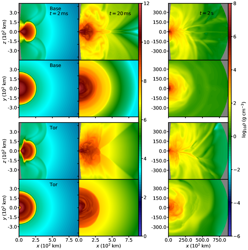
Figure 1: Density slices in the $x-z$ ($\phi=0$) and $x-y$ ($\theta=0$) plane of the base (top two rows) and base-tor (bottom two rows) models at t=2 ms (0.6 orbits at the initial torus density peak), 20 ms (6 orbits), and 2 s (600 orbits). The first two columns correspond to the early accretion and initial wind phase. Note the change in both colour table and length scale for the final column. Gray regions are outside the computational domain.

3.1 Overview of Torus Evolution in MHD

Our base and bhns runs, with a poloidal field embedded in the torus, show very similar evolution to previous runs in (GR)MHD. Within a few orbits, accretion onto the central object begins as magnetic pressure in the torus builds up via winding and onset of the MRI, disrupting hydrostatic equilibrium. In the base-tor run, accretion onto the torus begins as turbulence driven within the torus by the toroidal MRI generates poloidal field. Both runs then begin mass ejection as the poloidal MRI grows (Figure 1).

In contrast to hydrodynamic models, mass ejection begins on a timescale of $\sim$ms, forming “wings” of ejected material away from the midplane and rotation axis. More isotropic, thermally-driven ejecta takes over at $\sim$1 s, as neutrino emission has subsided and the disk enters an advective state. As material moves outward, it cools and releases the binding energy stored in $\alpha$-particles, increasing the internal energy of the fluid. Neutrino absorption, although subdominant energetically, is important in driving the evolution of $Y_{e}$. By $\sim$1 s, the torus has reached an equilibrium value of $Y_{e}$, and the cumulative mass outflow begins to plateau.

3.2 Mass Ejection in 3D Models

Table 2 shows the total unbound mass ejected by the end of each simulation (equation 17), and the extrapolation of of the mass outflow rate to infinity in time (equation 20), for all of our 3D models. The base and base-tor models eject $\sim 28\%$ and $\sim 42\%$ of the initial torus mass during the simulation, respectively, with the extrapolated mass ejected at late times being $\sim 40\%$ and $\gtrsim 50\%$. The bhns model ejects the least mass owing to the high compactness, with $\sim 5\%$ of the initial torus mass ejected by the end of the simulation. All 3D simulations show average velocities in the range $\langle v_{r}\rangle\sim(0.07-0.11)\,c$, and average electron fractions $\langle Y_{e}\rangle\sim 0.17-0.20$.

The mass accretion and outflow rates for all 3D models are shown in Figure 2. Each model begins to eject mass at a steeply rising rate, primarily due to MHD effects, which eventually reaches a plateau. After rising to a peak at time $\sim 1\,$s, the mass ejection rate then begins to decay as a power law with episodic ejection events. Figure 2 also shows that by this time, the cumulative mass ejected begins to plateau. Differences between models manifest as changes in the initial outflow time: the base-tor and bhns runs begin to eject matter $\sim 0.04\,$s and $0.02\,$s later than the base model, respectively. In the base-tor case, this delay is caused by the additional time required for the toroidal MRI to generate poloidal field, which then drives angular momentum transport. This is illustrated in Figure 3, which shows the evolution of the volume-integrated Maxwell stress for all 3D models. The bhns run has a deeper gravitational potential at the initial density maximum than the other runs (see §3.2.2), leading to more total energy input required to begin mass ejection (e.g., Fernández et al. 2020).

We also find that mass ejection peaks earlier in the base model than in the other two runs. The base-tor run reaches peak mass ejection around 0.1 s later than the base model at a somewhat larger outflow rate, but then decays with time following a power law slope of $\delta_{\mathrm{tor}}=1.45$, only $\sim$3% different than the base model slope $\delta_{\mathrm{base}}=1.50$. This qualitatively similar behaviour between poloidal and toroidal models is also found by Christie et al. (2019), although the initial conditions of their simulations lead to different quantitative values of $\delta$. Each 3D model has a different quantitative value of $\delta$, despite having the same late-time mass ejection mechanism. This variation can be attributed to physical differences in the disks and the timing of mass ejection. Each disk reaches maximum outflow at a phase in its evolution when the remaining disk mass, wind loss rate, and accretion rate are different relative to the initial disk mass and timescale of angular momentum transport in the disk. The initial time of mass ejection is also related to the range of electron fractions in the outflow. All runs produce a broad range of $Y_{e}$ in the ejecta, with a lower limit $Y_{e}\gtrsim 0.05$ (See §3.3.4).

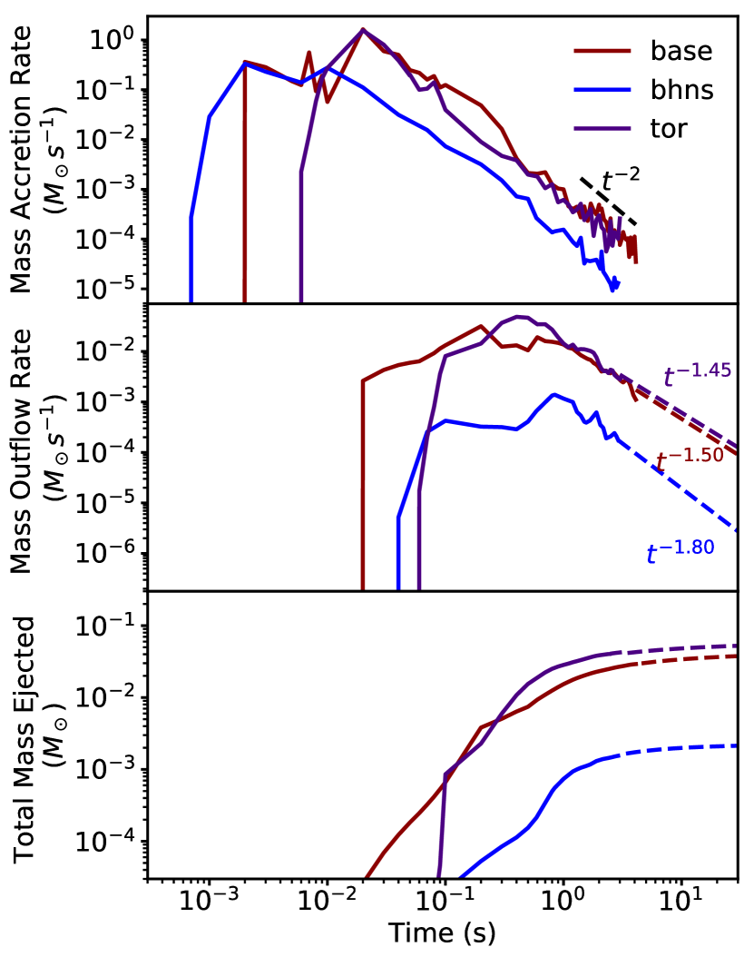
Figure 2: Top: mass accretion rate at the ISCO for all 3D models, as labeled. The dashed line shows a reference power-law dependence $t^{-2}$. Middle: unbound mass outflow rate at an extraction radius $r=10^{4}$ km, for all 3D models. Outflow rates are extrapolated with a power law (dashed lines), with the fiducial power law index shown for each curve (equation 20). Bottom: evolution of the cumulative unbound mass ejected (equation 17). Dashed lines show the result of using the same power-law extrapolation of the outflow rate after the end of the simulation (equation 20).

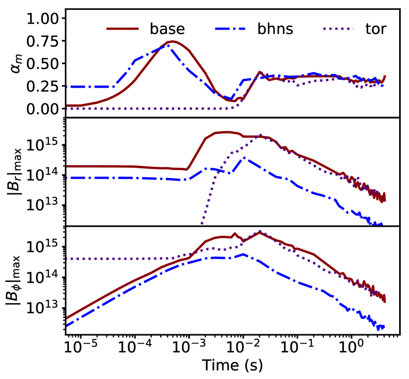
Figure 3: Top: Evolution of the volume-averaged Maxwell stress normalized by the volume-averaged magnetic pressure, $\alpha_{m}=\langle B_{r}B_{\phi}\rangle/\langle P_{\mathrm{mag}}\rangle$, a measure of radial angular momentum transport by magnetic forces (see Hawley 2000; Hawley & Krolik 2001 for a discussion). Middle: Evolution of the maximal magnitude of the radial magnetic field. Bottom: Evolution of the maximal magnitude of the azimuthal magnetic field.

3.2.1 Morphology

Kilonova emission is dependent on the ejecta morphology (e.g., Kasen et al. 2017; Kawaguchi et al. 2020, 2021; Korobkin et al. 2021; Heinzel et al. 2021), which can vary depending on the type of binary and mass ejection mechanism. The morphology of the disk outflow ejecta for the base and base-tor models is shown in the rightmost panel of Figure 1, showing a characteristic “hourglass” shape found in previous GRMHD simulations (e.g., Fernández et al. 2019a; Christie et al. 2019). This feature is robust across all our 3D models, as can be seen from the angular mass outflow histograms in Figure 4. Model base-tor ejects $50\%$ less mass with $v\gtrsim 0.25\,c$ and within $\sim\pi/4$ of the rotation axis than model base, and no ejecta in this velocity range is produced within $\sim\pi/4$ of the equatorial plane. In contrast, models base and bhns have a much wider distribution of fast/early ejecta, extending down to within $\pi/6$ of the rotation axis. This implies that the morphology of the highest velocity ejecta is dependent on the initial condition of the torus, with the compactness of the disk having little effect on outflow geometry. This result is supported by the results of (Christie et al., 2019), as well as those of (Siegel & Metzger, 2018) in their discussion of the initial transient phase.

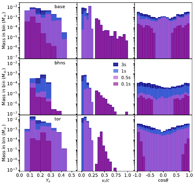
Figure 4: Total unbound mass ejected by our 3D models, as labeled, sorted into bins based on electron fraction $Y_{e}$,radial velocity $v_{r}$, and polar angle $\theta$. The bin sizes are $\Delta Y_{e}=0.05$, $\Delta v_{r}/c=0.05$, and $\Delta\cos\theta=0.1$, where $\cos\theta=0$ is the midplane.

3.2.2 Compactness

We find that the fraction of the initial disk mass ejected decreases with increasing disk compactness (model bhns), following the same trend as the hydrodynamic results of Fernández et al. (2020). This shows that the additional mass ejected by MHD effects relative to pure viscous hydrodynamics also decreases with increasing disk compactness. Figure 4 shows that the fastest ejecta ($t<0.1s$) becomes a smaller fraction of the total mass ejected, with the majority of the disk outflow ensuing after $1$ s. This change can be attributed to multiple differences with the base model: the gravitational potential is deeper by a factor $\sim 2$ at the density maximum, the ISCO of the BH is closer to the torus density maximum (see, e.g., Figure 2), and the initially lower density torus emits an order of magnitude less neutrino luminosity and is more transparent to neutrinos. Nevertheless, the different disk structure results in a shorter neutrino cooling time at the initial density peak in the bhns model ($1$ ms) relative to the base model ($2$ ms). Thus, at early times ($t<0.1s$) when neutrino cooling is strong, disk material is more bound in the bhns than in the base case.

We note a sharp drop in mass ejected with $Y_{e}\sim 0.3$ for the base model, also found in Fernández et al. (2020), which can be attributed to the larger relative importance of neutrino absorption in more massive tori. For a neutron-rich disk where neutrino absorption dominates the evolution of $Y_{e}$, the process $\nu_{e}+n\rightarrow e^{-}+p$ occurs more frequently than its inverse, increasing the net $Y_{e}$ (Siegel & Metzger, 2018; Fernández et al., 2020; Most et al., 2021).This trend is also found by Just et al. (2022) with a significantly more advanced neutrino scheme - a broader distribution in $Y_{e}$ corresponds to more absorption (see their Figure 13). Similar 2D axisymmetric simulations by Shibata & Sekiguchi (2012) yield neutrino luminosities that decrease from $10^{52}$ erg s^-1 to $10^{51}$ erg s^-1 as the BH mass increases by from $3M_{\odot}$ to $6M_{\odot}$. We find a very similar trend as we change the compactness.

3.3 Mass Ejection in 2D: Sensitivity to Physics Inputs

3.3.1 Dimensionality

Measuring unbound ejecta by the end of each simulation, the base-2D model ejects a factor of $\sim 2$ more mass than the equivalent base run in 3D, despite running for $1.4\,$s instead of $3\,$s. The evolution is qualitatively similar for the first $\sim 1\,$s, until the axisymmetric torus becomes dominated by magnetic pressure and is disrupted, at which point we end the simulation. Quantitatively, model base-2D produces a higher mass outflow rate at all times, in particular more ejecta with velocities $\gtrsim 0.25\,c$. We attribute this enhanced mass ejection to the lower accretion rate onto the BH in axisymmetry given the suppression of the MRI, with divergence in the evolution from the 3D case starting at $\sim 20$ ms. With less accretion, the larger amount of matter in the torus results in a higher outflow rate, given that the same outflow driving processes operate in 2D and in 3D.

3.3.2 Spatial Resolution

To quantify uncertainties due to spatial resolution, we run versions of model base-2D at half and twice the resolution in both the radial and polar directions. The high-resolution model is evolved until $0.5$ s, probing the early, magnetically-driven phase, and the half-resolution model is evolved until $1$ s, which includes the radiatively-inefficient phase of mass ejection. Mass ejection up to $1$ s is $\sim 10$% higher in the standard resolution model relative to the low-resolution model. We thus associate an uncertainty of 10% to our mass ejection numbers due to spatial resolution. The growth of the toroidal magnetic field is identical during both the magnetic winding and MRI growth phase in all models until $3$ ms, when the maximum value of toroidal magnetic field saturates at $2\times 10^{15}$ G. We find a 0.5% difference in the saturation value of $|B_{\phi}|$ between the standard and high resolution runs, and a 5% lower saturation value comparing the low to standard resolution run. Thereafter, the maximum of $|B_{\phi}|$ undergoes stochastic fluctuations with amplitude of order unity until a dissipation phase begins at $\sim 30$ ms. The standard and high-resolution models remain consistent within fluctuations.

3.3.3 Nuclear Recombination

Comparing mass ejection from models base-2d (with recombination) and base-norec (without recombination), we find that nuclear recombination remains a subdominant effect until the end of our 2D simulation at $1.4\,$s. Before $0.5\,$s, energy input from nuclear recombination increases the mass-averaged velocity of ejecta, resulting in a noticeable decrease in mass ejected at $\sim 0.3\,c$ and a increase at $\sim 0.25\,c$ in model base-norec compared to model base. After $\gtrsim 0.5\,$s, comparatively less mass is ejected in model base-norec due to the lack of recombination heating. In other words, mass which would have been ejected in the initial MHD-driven phase is instead ejected slower and at a later time, indicating that the net effect of nuclear recombination is to make matter less gravitationally bound and thus easier to eject by magnetic forces at early times. We find an almost identical distribution in electron fraction, skewed to a slightly lower average value since less mass is ejected later when the charged current weak interactions have already raised the $Y_{e}$.

3.3.4 Neutrino Absorption

Inclusion of neutrino absorption results in additional mass ejection by a factor of $\sim 2$ relative to a model without it (base-noirr), and a negligible effect on the mass ejected at $t<0.1$ s, when magnetic stresses dominate. The energy input from neutrino absorption causes additional mass to become marginally unbound, extending the distribution in velocity space to slower outflow. However, since more mass is ejected, neutrino absorption produces a decrease by $0.05\,c$ in the mass averaged velocity. Turning off neutrino absorption skews the electron fraction of the ejecta to lower values, with more mass (factor of 2) being ejected at all times with $Y_{e}<0.1$, and 2 orders of magnitude less ejecta with $Y_{e}>0.4$.

3.4 Comparison to previous work

The ejected masses and velocities from our 3D models are in broad agreement with comparable simulations (Siegel & Metzger, 2018; Miller et al., 2019; Fernández et al., 2019a; Christie et al., 2019; Just et al., 2022). The base run is qualitatively closest to the model of Siegel & Metzger (2018), which lacks neutrino absorption, and to the MHD model of Just et al. (2022), which has a less massive torus ($0.01M_{\odot}$). Siegel & Metzger (2018) find that 16% of the torus is ejected during 381 ms of evolution, and Just et al. (2022) that 20% of the initial torus mass is ejected during 2.1 s. Our base model ejects a higher fraction of the initial disk mass due to the difference in compactness as well as a longer simulation time. Relative to the long-term GRMHD simulation of Fernández et al. (2019a), which employed an initial field geometry conducive to a magnetically-arrested disk (MAD, e.g., Tchekhovskoy et al. 2011), ran for a longer time ($\sim 10$ s), and did not include neutrino absorption, our base run ejects $\sim 20\%$ less mass by the end of the simulation at 3s. Our extrapolated ejected masses are comparable to that from this longer run, with other differences explainable by the difference in compactness and initial field geometry. The weak poloidal (SANE) model from Christie et al. (2019) is run for the same amount of time as our base run but with an initially weaker field, and also ejects $\sim 30\%$ of the torus mass during the simulation, despite not including neutrino absorption.

The toroidal run of Christie et al. (2019) ejects 3% less mass than their weak poloidal (MAD) run, whereas we find 15% more mass ejection in our base-tor (toroidal) model relative to our base (poloidal) model. We do find a lower average velocity (by $\sim 0.02\,c$) in the base-tor model relative to our base model, same as they do. Christie et al. (2019) find that their toroidal model begins mass ejection at almost the same time as their weak poloidal run, and find a more sustained period of mass ejection from $\sim 0.01-0.05$ s in the toroidal model. Comparatively, we find that mass ejection in our base-tor model begins later and quickly rises to peak at a value higher than that of the poloidal simulation. This difference in dynamics could be attributed to a comparatively stronger toroidal magnetic field ($\beta\sim 0.01-2$ in the initial torus) and the effect of neutrino absorption. We do not vary the initial field strength in our simulations, as a lower field strength would require more cells to properly resolve the MRI. We can speculate on how lowering the field strength would change our outflows by comparing to the results of Christie et al. (2019). They find that lowering the field strength reduces the initial ($t\lesssim 0.5$ s) outflows driven by magnetic stresses, but the late-time thermal outflows are nearly identical. The effects on our (SANE) field configuration would likely be similar, but less prominent, given that their MAD configuration is optimized for producing magnetic outflows.

The work of Miller et al. (2019) utilizes the same initial conditions as our base model but with a more advanced neutrino scheme to treat neutrino emission and absorption. We find a similar amount of mass ejected by 100ms of evolution ($\sim 2\times 10^{-3}M_{\odot}$), indicating broad agreement despite the difference in neutrino schemes.

Utilizing a mean field dynamo to address the suppression of MRI in 2D, Shibata et al. (2021b) run resistive MHD simulations of high compactness toroidal disks. They find $\sim 10-20\%$ of the initial disk mass is ejected over $\gtrsim 4\,$s with an average electron fraction $\langle Y_{e}\rangle\sim 0.25-0.35$, in broad agreement with our findings. Notably, they find that mass ejection begins $\gtrsim 500$  ms later than in our toroidal run, although this delay can be attributed to the high compactness of their models.

The recent GRMHD simulations of Hayashi et al. (2021) start from the inspiral of a 1.35$M_{\odot}$ NS and a 5.4 or 8.1 $M_{\odot}$ BH and evolve the remnant for up to $2$ s, including neutrino leakage and absorption. They find qualitatively similar results when compared to our runs, albeit with much larger tori masses post-merger ($\sim 0.2-0.3M_{\odot}$). The fraction of the torus mass ejected is also comparable to our bhns runs, as $\sim 10\%$ of their tori is ejected in the first 1 s, with a broad distribution in both electron fraction and velocity. Discounting dynamical ejecta, they find a peak electron fraction $Y_{e}\sim 0.25-0.35$ and post merger outflow velocities of $v\lesssim 0.08\,c$, in good agreement with our results. They find outflows starting at $\gtrsim 200$ ms later than our bhns model, however the initial tori in their simulations are in a deeper potential well, and form with an initially toroidal field, both of which we find delay outflows in comparison to our base model.

By analyzing the net specific energy of tracer particles, Siegel & Metzger (2018) find that nuclear recombination of $\alpha$-particles plays a key role in unbinding matter in the disk outflow (in a simulation that does not include neutrino absorption). Our 2D model base-norec which has nuclear recombination turned off but includes neutrino absorption, ejects only slightly less mass than our base-2D run indicating that under these circumstances nuclear recombination is a sub-dominant effect. It remains to be tested whether recombination will remain sub-dominant in a fully 3D simulation that includes neutrino absorption and runs for a long time ($\gg 1$ s).

Our 2D model without neutrino absorption (base-noirr) ejects a factor $\sim 2$ less mass than the base-2D model. This difference is significantly larger than that found in models that employ viscous hydrodynamics, which typically find that neutrino absorption is dynamically sub-dominant for mass ejection (e.g., Fernández & Metzger 2013; Just et al. 2015). This also inconsistent with the 3D MHD run of Just et al. (2022), who find that turning off neutrino absorption results in a 2.5% increase in mass ejection relative to the initial torus mass, although they use a different neutrino leakage scheme and a less massive torus that is more transparent to neutrinos. Our results are limited by the use of axisymmetry for these simulations, but suggest that neutrino absorption could indeed be more significant for the dynamics of mass ejection and motivates further studies in 3D.

4 Summary and Discussion

We have run long-term 3D MHD simulations to explore mass ejection from BH-tori systems formed in neutron star mergers. The publicly available code FLASH4.5 has been extended to allow its unsplit MHD solver to work on non-uniform spherical coordinates in 3D (Appendix A, B). All of our models include a physical EOS, neutrino emission and absorption via a leakage scheme with disk-lightbulb irradiation (Appendix C), and treat the gravity of the BH with a pseudo-Newtonian potential. Our 3D models employ different initial magnetic field geometries and disk compactnesses. We have also carried out axisymmetric models that suppress the nuclear recombination and neutrino absorption source terms.

The disk outflows from our 3D models exhibit a broad distribution in electron fraction and ejection polar angle (Figure 4), with a typical hourglass morphology (Figure 1). The tori eject matter with a bimodal distribution in velocity (Figure 4) associated with two different mass ejection phases: MHD stresses power early time ($t<0.1$ s) high velocity ($v\gtrsim 0.25\,c$) ejecta, and late-time ($t\sim$ s) “thermal” ejection provides the majority of mass outflows centered around $vsim0.1\,c$.

We find that imposing an initially toroidal field configuration ejects $\sim$15% more of the initial torus mass than the standard SANE poloidal field of similar maximal field strength (Figure 2, Table 2). However, the toroidal model ejects an order of magnitude less ejecta in the first 100 ms of evolution (Figure 4), comprising all of the ejecta travelling at velocities $v\gtrsim 0.25\,c$. The high-velocity ejecta is suppressed by the additional time it takes for dynamo action to convert toroidal into large-scale poloidal fields, which then drives radial angular momentum transport.

Increasing the disk compactness to values expected for typical BH-NS mergers results in significantly less mass ejection relative to our base (NS-NS) model, beginning at a later time and decaying at a faster rate. Comparing to the viscous hydrodynamic models of Fernández et al. (2020), we find the same overall trend of decreased mass ejection with increasing disk compactness. Model bhns has the same initial torus and BH configuration as their model b08d03: by 4 s, our 3D MHD simulation has ejected $5.5\%$ of the initial torus mass, while the viscous hydrodynamic equivalent has ejected only $1.9\%$ of the initial disk mass by the same time. The hydrodynamic model goes on to eject $5.0\%$ of the initial disk mass after $12\,$ s of evolution, with mass ejection peaking at $2.3$ s but remaining non-negligible until later times. The extrapolated outflow for our 3D MHD model bhns predicts $6-8\%$ of the initial torus mass, which is consistent with the previously-found enhancement in mass ejection by MHD relative to viscous hydrodynamics at smaller compactnesses when evolving both to $\sim 10$ s (Fernández et al., 2019a). Our results inform analytic fits to fractions of the initial disk mass ejected like that of Raaijmakers et al. (2021), which has the enhancement in mass ejection due to magnetic effects relative to viscous hydrodynamics as a free parameter. More 3D MHD simulations at different compactness and with various initial magnetic field geometries are needed to improve the predictive power of these fits.

Our axisymmetric models that vary the physics show that nuclear recombination is a sub-dominant effect, while neutrino absorption can make a significant difference in mass ejection. Inclusion of neutrino absorption produces a shift of the velocity distribution at late times, down by $\sim 0.05\,c$, with negligible effects at early times ($t<0.1\,$). In the absence of neutrino absorption, the distribution of electron fraction shifts to include additional material with $Y_{e}<0.1$ and exclude $Y_{e}>0.4$. Nuclear recombination deposits additional energy into the already unbound outflows at $t\sim 0.1\,$s, resulting in ejecta with moderately higher velocities, but its absence only decreases the total ejecta mass by 1%. Inclusion of $r$-process heating by the formation of heavier nuclei can further speed up the ejecta at late times (Klion et al., 2022). Proper characterization of the effect of neutrino absorption and nuclear recombination on the mass ejection dynamics and composition must be done with full 3D simulations, which unfortunately still remain expensive computationally.

Our base and base-tor models have initial conditions consistent with the post-merger system of the observed NS-NS merger GW170817. We find that although these 3D models can eject lanthanide-free material ($Y_{e}>0.25$) with velocities inferred from kilonova modelling, $v\gtrsim 0.25\,c$, there is insufficient mass in the outflows to match observations (e.g., Kasen et al. 2017; Villar et al. 2017) with the disk outflow alone. The inclusion of a finite-lived remnant in our base model is a promising way to produce more lanthanide-free ejecta at the required velocities (e.g., Fahlman & Fernández 2018).

The main limitations of our work are the approximations made for modelling neutrino radiation transport on the necessary timescales. Prior research into the effectiveness of neutrino schemes have shown that the differences between two-moment (M1) and Monte Carlo (MC) schemes can result in a $\sim 20$% uncertainty in neutrino luminosity, translating to a difference of 10% in outflow electron fraction (Foucart et al., 2020). Comparison between M1 and the leakage scheme of Ardevol-Pulpillo et al. (2019) (which our scheme is based on, see Appendix C) shows a further 10% uncertainty in neutrino luminosities, and a comparison of leakage+M0 to M1 schemes shows that leakage schemes tend to decrease the average $Y_{e}$, but with a minimal effect on nucleosynthetic yields (Radice et al., 2021). The exclusion of relativistic effects implies that we cannot accurately model jet formation, but the effects of these approximations on mass ejection and composition are likely minimal, since the relevant processes operate far from the BH. The leading order special relativistic corrections to the MHD equations are $\sim v/c$ for $v<c$, hence we estimate uncertainties associated with our fastest ejecta to be at least of the same order (e.g., 50% for matter with $v_{r}/c=0.5$, etc.). The bulk of mass ejection has $v_{r}/c<0.1$, and thus uncertainties due to Newtonian physics should be on the order of 10%, comparable to those due to spatial resolution.

Data Availability

The data underlying this article will be shared on reasonable request to the corresponding author.

Appendix A MHD in Spherical Coordinates

In this appendix we extend the work done in Fahlman (2019), where the default dimensionally-unsplit hydrodynamic solver in FLASH4 (Lee, 2013) was modified to work in non-uniform 3D spherical coordinates. Here we add the solution of the ideal MHD equations by including contributions at each face from transverse and diagonal fluxes. To ensure the divergence-free evolution of magnetic fields, FLASH4.5 solves the induction equation via the constrained transport (CT) method of Evans & Hawley (1988) on a uniform staggered mesh. We also modify the default CT method to work in non-uniform 3D spherical coordinates.

A.1 Governing Equations of Magnetohydrodynamics

The ideal MHD equations are those of mass, momentum, and energy conservation (equations 1-3 without source terms) together with the induction equation (5). Note that in FLASH the induction equation is implemented as

$$\frac{\mathrm{d}\mathbf{B}}{\mathrm{d}t}+\vec{\nabla}\cdot{(\mathbf{B}\otimes\mathbf{v}-\mathbf{v}\otimes\mathbf{B})}=0$$ (21)

which has the opposite sign as equation (5). For the rest of this Appendix, we will use this form of the induction equation for consistency with the available literature on FLASH.

The conservation equations are written in terms of a vector of conserved variables $\mathbf{U}$, a tensor of associated fluxes $\mathcal{F}$, and a vector of source terms $\mathbf{S}$,

$$\frac{\partial\mathbf{U}}{\partial t}+\vec{\nabla}\cdot{\mathcal{F}}=\mathbf{S}.$$ (22)

Writing out the associated fluxes in the radial, polar, and azimuthal direction as $\mathbf{F}$, $\mathbf{G}$, and $\mathbf{H}$ respectively, we obtain

$$\frac{\partial\mathbf{U}}{\partial t}+\frac{1}{r^{2}}\frac{\partial(r^{2}\mathbf{F})}{\partial r}+\frac{1}{r\sin\theta}\frac{\partial(\sin\theta\mathbf{G})}{\partial\theta}+\frac{1}{r\sin\theta}\frac{\partial\mathbf{H}}{\partial\phi}=\mathbf{S},$$ (23)

where (Lee, 2013)

$$\mathbf{U}=\begin{pmatrix}\rho\\ \rho v_{r}\\ \rho v_{\theta}\\ \rho v_{\phi}\\ B_{r}\\ B_{\theta}\\ B_{\phi}\\ \rho E\end{pmatrix},\qquad \mathbf{F}=\begin{pmatrix}\rho v_{r}\\ \rho v_{r}^{2}+P-B_{r}^{2}\\ \rho v_{r}v_{\theta}-B_{r}B_{\theta}\\ \rho v_{r}v_{\phi}-B_{r}B_{\phi}\\ 0\\ v_{r}B_{\theta}-v_{\theta}B_{r}=-E_{\phi}\\ v_{r}B_{\phi}-v_{\phi}B_{r}=E_{\theta}\\ v_{r}(\rho E+P)-B_{r}(\mathbf{v}\cdot\mathbf{B})\end{pmatrix},$$

$$\mathbf{G}=\begin{pmatrix}\rho v_{\theta}\\ \rho v_{\theta}v_{r}-B_{\theta}B_{r}\\ \rho v_{\theta}^{2}+P-B_{\theta}^{2}\\ \rho v_{\theta}v_{\phi}-B_{\theta}B_{\phi}\\ v_{\theta}B_{r}-v_{r}B_{\theta}=E_{\phi}\\ 0\\ v_{\theta}B_{\phi}-v_{\phi}B_{\theta}=-E_{r}\\ v_{\theta}(\rho E+P)-B_{\theta}(\mathbf{v}\cdot\mathbf{B})\end{pmatrix},$$

$$\mathbf{H}=\begin{pmatrix}\rho v_{\phi}\\ \rho v_{\phi}v_{r}-B_{\phi}B_{r}\\ \rho v_{\theta}v_{\phi}-B_{\theta}B_{\phi}\\ \rho v_{\phi}^{2}+P-B_{\phi}^{2}\\ v_{\phi}B_{r}-v_{r}B_{\phi}=-E_{\theta}\\ v_{\phi}B_{\theta}-v_{\theta}B_{\phi}=E_{r}\\ 0\\ v_{\phi}(\rho E+P)-B_{\phi}(\mathbf{v}\cdot\mathbf{B})\end{pmatrix}.$$ (24)

In conservative mesh-based codes like FLASH, the conserved variables are evolved by discretizing (23) in both time and space. This means that we evolve each variable by taking a volume average over the cell, and then advance the volume-averaged variable using the corresponding fluxes at the faces. Using the indices $\{i,j,k\}$ to enumerate cells in the radial, polar, and azimuthal directions, respectively, using half integer indices to denote values at cell faces ($\pm\frac{1}{2}$), and using the index $n$ to denote time step, the conservative system of equations can be written concisely as

$$\langle\mathbf{U}^{n+1}_{i,j,k}\rangle=\langle\mathbf{U}^{n}_{i,j,k}\rangle-\frac{\Delta t}{V}\bigg{[} (A_{i-\frac{1}{2}}\mathbf{F}_{i-\frac{1}{2}}-A_{i+\frac{1}{2}}\mathbf{F}_{i+\frac{1}{2}})$$

$$- (A_{j-\frac{1}{2}}\mathbf{G}_{j-\frac{1}{2}}-A_{j+\frac{1}{2}}\mathbf{G}_{j+\frac{1}{2}})$$

$$- (A_{k-\frac{1}{2}}\mathbf{H}_{k-\frac{1}{2}}-A_{k+\frac{1}{2}}\mathbf{H}_{k+\frac{1}{2}})\bigg{]}$$

$$+ \Delta t\langle\mathbf{S}\rangle,$$ (25)

where $A_{\{i,j,k\}\pm\frac{1}{2}}$ is the area of the cell face perpendicular to the denoted direction, $V$ is volume of the cell, $\langle\mathbf{S}\rangle$ is the volume-averaged source term, and $\Delta t=t^{n+1}-t^{n}$ is the timestep. We have used Gauss’s Law,

$$\iiint_{V}\vec{\nabla}\cdot{\mathbf{F}}\mathrm{d}V=\oiint_{A}\mathbf{F}\cdot\mathrm{d}\mathbf{A},$$ (26)

to relate volume-averaged conserved variables $\langle U\rangle$ to the face-centered fluxes. To make the conservative variable update consistent with curvilinear coordinates, we compute the discretized cell face areas and volumes for arbitrarily spaced spherical cells (Fahlman, 2019).

A.2 Geometric Source Terms in Spherical Coordinates

The geometric source terms arise when taking covariant derivatives of second rank tensors, often referred to as a tensor divergence. These terms take the physical form of fictitious forces, and only arise in the equations for vector quantities. The scalar energy and density evolution equations therefore do not have source terms. For a tensor, $T$, in spherical coordinates the divergence is written as (see Fahlman 2019, or Mignone et al. 2005 for a separate derivation)

$$\vec{\nabla}\cdot{T}=\begin{pmatrix}\nabla_{r}T\\ \nabla_{\theta}T\\ \nabla_{\phi}T\end{pmatrix},$$ (27)

where we can define the divergences in each individual direction as

$$\nabla_{r}T=\bigg{(}\frac{1}{r^{2}}\frac{\partial(r^{2}T^{rr})}{\partial r}+\frac{1}{r\sin\theta}\frac{\partial(\sin\theta T^{\theta r})}{\partial\theta}+\frac{1}{r\sin\theta}\frac{\partial T^{\phi r}}{\partial\phi}-\\ \frac{T^{\theta\theta}+T^{\phi\phi}}{r}\bigg{)},$$ (28)

$$\nabla_{\theta}T=\bigg{(}\frac{1}{r^{2}}\frac{\partial(r^{2}T^{r\theta})}{\partial r}+\frac{1}{r\sin\theta}\frac{\partial(\sin\theta T^{\theta\theta})}{\partial\theta}+\frac{1}{r\sin\theta}\frac{\partial T^{\phi\theta}}{\partial\phi}+\\ \frac{T^{\theta r}}{r}-\frac{T^{\phi\phi}}{r}\cot\theta\bigg{)},$$ (29)

$$\nabla_{\phi}T=\bigg{(}\frac{1}{r^{2}}\frac{\partial(r^{2}T^{r\phi})}{\partial r}+\frac{1}{r\sin\theta}\frac{\partial(\sin\theta T^{\theta\phi})}{\partial\theta}+\frac{1}{r\sin\theta}\frac{\partial T^{\phi\phi}}{\partial\phi}+\\ \frac{T^{\phi r}}{r}+\frac{T^{\phi\theta}}{r}\cot\theta\bigg{)}.$$ (30)

Explicitly applying the divergences (28)-(30) to the dyads in the momentum and induction equations (2 and 5) yields the source term vector in equation (22)

$$\mathbf{S}=\begin{pmatrix}0\\ \dfrac{\rho(v_{\theta}^{2}+v_{\phi}^{2})-B_{\theta}^{2}-B_{\phi}^{2}}{r}\\[8.61108pt] -\dfrac{\rho v_{r}v_{\theta}-B_{r}B_{\theta}}{r}+\dfrac{\cot{\theta}(\rho v_{\phi}^{2}-B_{\phi}^{2})}{r}\\[8.61108pt] -\dfrac{\rho v_{r}v_{\phi}-B_{r}B_{\phi}}{r}-\dfrac{\cot\theta(\rho v_{\phi}v_{\theta}-B_{\phi}B_{\theta})}{r}\\ 0\\ \dfrac{(B_{\theta}v_{r}-B_{r}v_{\theta})}{r}\\[8.61108pt] \dfrac{(B_{\phi}v_{r}-B_{r}v_{\phi})}{r}+\dfrac{(B_{\phi}v_{\theta}-B_{\theta}v_{\phi})\cot\theta}{r}\\ 0\end{pmatrix}.$$ (31)

The source terms have to be volume averaged according to

$$\langle\mathbf{S}\rangle=\frac{1}{V}\iiint_{V}\mathbf{S}(r,\theta)\mathrm{d}V.$$ (32)

for use in the discretized conservative update equation (A.1). Since conservative mesh schemes store hydrodynamic variables as volume averages, we make the approximation of taking them out of the integral in equation (32). The remaining terms contain either a $r^{-1}$ or $\cot\theta$ dependence, which are integrated analytically to get the volume-averaged source term vector

$$\langle\mathbf{S}\rangle=\dfrac{3\Delta r^{2}}{2\Delta r^{3}}\begin{pmatrix}0\\ \rho(v_{\theta}^{2}+v_{\phi}^{2})-B_{\theta}^{2}-B_{\phi}^{2}\\[8.61108pt] -\rho v_{r}v_{\theta}-B_{r}B_{\theta}+\dfrac{\Delta\sin\theta}{\Delta\cos\theta}(\rho v_{\phi}^{2}-B_{\phi}^{2})\\[8.61108pt] -\rho v_{r}v_{\phi}-B_{r}B_{\phi}-\dfrac{\Delta\sin\theta}{\Delta\cos\theta}(\rho v_{\phi}v_{\theta}-B_{\phi}B_{\theta})\\[8.61108pt] 0\\ (B_{\theta}v_{r}-B_{r}v_{\theta})\\[8.61108pt] (B_{\phi}v_{r}-B_{r}v_{\phi})+\dfrac{\Delta\sin\theta}{\Delta\cos\theta}(B_{\phi}v_{\theta}-B_{\theta}v_{\phi})\\[8.61108pt] 0\end{pmatrix},$$ (33)

where the coordinate differences are defined as

$$\Delta r^{2} =r^{2}_{i+\frac{1}{2}}-r^{2}_{i-\frac{1}{2}},$$ (34)

$$\Delta r^{3} =r^{3}_{i+\frac{1}{2}}-r^{3}_{i-\frac{1}{2}},$$ (35)

$$\Delta\cos\theta =\cos\theta_{j+\frac{1}{2}}-\cos\theta_{j-\frac{1}{2}},$$ (36)

$$\Delta\sin\theta =\sin\theta_{j+\frac{1}{2}}-\sin\theta_{j-\frac{1}{2}}.$$ (37)

These are the source terms used in the update of conserved variables (equation A.1).

A.3 Fluxes and Primitive Variables in Spherical Coordinates

Before the conservative update (equation A.1) can be performed, the fluxes at the face must be known. Here we provide only the information needed to adjust the reconstruction of fluxes for spherical coordinates. The discretization and methods used in FLASH to extend variables to the face and construct appropriate Riemann states can be found in Lee (2013). By default, FLASH employs a piecewise linear MUSCL-Hancock method (Colella, 1985) to reconstruct the so-called cell-centered primitive variables,

$$\boldsymbol{\mathcal{V}} =(\rho,v_{r},v_{\theta},v_{\phi},B_{r},B_{\theta},B_{\phi},P_{\mathrm{gas}})^{T},$$ (38)

instead of the conserved variables, to the faces. The corresponding primitive system of equations is derived using the chain rule to expand the divergence in the conservative system. The primitive system is utilized in part because it has a quasi-linear form, which is written out in spherical coordinates as

$$\frac{\partial\boldsymbol{\mathcal{V}}}{\partial t} +\mathbf{M}_{r}\frac{\partial\boldsymbol{\mathcal{V}}}{\partial r}+\mathbf{M}_{\theta}\frac{1}{r}\frac{\partial\boldsymbol{\mathcal{V}}}{\partial\theta}+\mathbf{M}_{\phi}\frac{1}{r\sin\theta}\frac{\partial\boldsymbol{\mathcal{V}}}{\partial\phi}=\mathbf{S}_{p},$$ (39)

where the matrices $\mathbf{M}_{r},\mathbf{M}_{\theta},\mathbf{M}_{\phi}$ can be found in Lee & Deane (2009) and Lee (2013). Explicitly expanding all the spatial and temporal derivatives of the conseravative equations (1, 2, 3, 21) in spherical coordinates results in a source term vector for the primitive system of variables given by

$$\mathbf{S}_{p}=\begin{pmatrix}-\rho\bigg{(}\dfrac{2v_{r}+v_{\theta}\cot{\theta}}{r}\bigg{)}\\[8.61108pt] \dfrac{(v_{\theta}^{2}+v_{\phi}^{2})-(B_{\theta}^{2}+B_{\phi}^{2})/\rho}{r}\\[8.61108pt] -\dfrac{v_{r}v_{\theta}-B_{r}B_{\theta}/\rho}{r}+\dfrac{\cot{\theta}(v_{\phi}^{2}-B_{\phi}^{2}/\rho)}{r}\\[8.61108pt] -\dfrac{v_{r}v_{\phi}-B_{r}B_{\phi}/\rho}{r}-\dfrac{\cot\theta(v_{\phi}v_{\theta}-B_{\phi}B_{\theta}/\rho)}{r}\\[8.61108pt] -\dfrac{\cot\theta(B_{\theta}v_{r}-B_{r}v_{\theta})}{r}\\[8.61108pt] -\dfrac{(B_{\theta}v_{r}-B_{r}v_{\theta})}{r}\\[8.61108pt] \dfrac{(B_{\phi}v_{r}-B_{r}v_{\phi})}{r}\\[8.61108pt] -\gamma_{1}P_{\mathrm{gas}}\bigg{(}\dfrac{2v_{r}+v_{\theta}\cot{\theta}}{r}\bigg{)}\end{pmatrix}.$$ (40)

These are the source terms implemented in the reconstruction of cell-centered variables to the faces, along with the geometrically correct lengths, in equation (39).

A.4 Constrained Transport

Magnetic fields require an update method different from conserved quantities, as the induction equation does not explicitly require that the solenoidal constraint,

$$\vec{\nabla}\cdot{\mathbf{B}}=0,$$ (41)

is satisfied. To satisfy this constraint, fields are taken to be averaged over cell faces, and the induction equation is written as

$$\oiint\frac{\partial\mathbf{B}}{\partial t}\cdot\mathrm{d}\mathbf{A} =\oiint-\nabla\times\mathbf{E}\cdot\mathrm{d}\mathbf{A}.$$ (42)

Applying Stokes’ theorem, using the definition of magnetic fields as area-averaged, and discretizing the resulting line integral as a sum, we arrive at the Newtonian form of CT (Evans & Hawley, 1988)

$$\mathbf{B}\cdot\mathbf{A} =-\frac{\Delta t}{2}\sum_{\mathrm{edges}}\mathbf{E}\cdot\Delta\boldsymbol{\ell}.$$ (43)

To perform the summation, we need the electric fields around each edge of the cell. These are found by Taylor expanding the face centered electric fields, which are obtained from the fluxes of conserved magnetic variables (equation A.1) in the reconstruction step, and using Ohm’s law in ideal MHD

$$\mathbf{E}=-\mathbf{v}\times\mathbf{B}.$$ (44)

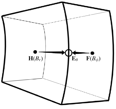
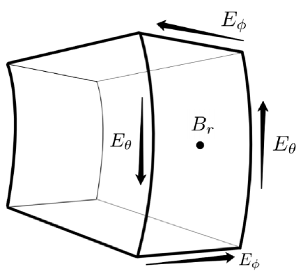
Figure 5: Left: Schematic representation of the method to obtain the electric field at cell edges for the CT method (equation 43). The electric fields at cell faces are obtained using Ohm’s law in ideal MHD (equation 44) from the magnetic fluxes at the face (solid black circles). The electric fields are then Taylor-expanded to the cell edge using finite derivatives (equations [46]-[47]). The expanded values are then averaged using upwinding for numerical stability (open circle, see text). Two additional symmetric expansions to the same edge have been left out for visual clarity. Right: Schematic description of the reconstruction of the face-centered radial magnetic field by adding up the total contribution from electric fields along each of the cell edges (equation 43).

Each flux contains 2 electric fields, one in each transverse direction. At each edge there will be 4 independent fluxes that can be used to find the electric field at that point (Figure 5 shows two of the fluxes) Conventionally, all 4 contributions are included, which can be numerically unstable (e.g., Tóth 2000; Mignone & Del Zanna 2021). Fortunately, FLASH includes an option to only use the upwind fluxes (flux vectors which have a positive mass flux) to construct the electric fields (e.g., White et al. 2016). We find that this upwinded method is necessary to preserve numerical stability when using FLASH to evolve a magnetized torus in 3D spherical coordinates, despite not being a default option. This is also found by Kuroda et al. (2020), who note that in the regions of their core-collapse supernova setup where matter is supersonically advecting (analogous to the torus), the upwind method is necessary for stability. While no additional work is needed to implement the upwinding in spherical coordinates, the Taylor expansion for expanding the face fluxes to cell edges must be updated to account for non-uniform grid spacing. The Taylor expansion uses second-order finite differences to determine the approximate value at face edges. For example, the expansion in an arbitrary $i^{\mathrm{th}}$ direction is

$$E_{i\pm\frac{1}{2},j,k}=E_{i,j,k}\pm\Delta\ell_{i\pm\frac{1}{2}}\frac{\partial E}{\partial\ell}+(\Delta\ell_{i\pm\frac{1}{2}})^{2}\frac{1}{2}\frac{\partial^{2}E}{\partial\ell^{2}},$$ (45)

where $\Delta\ell_{i\pm 1/2}$ corresponds to the distance from the center of the cell to the $i^{\mathrm{th}}$ face. Writing the spatial derivatives as cell-centered finite differences, where $\Delta\ell_{\pm}$ is the distance from the center of the cell $i$ to the cell centers above and below ($i\pm 1$), yields

$$\frac{\partial E}{\partial\ell} =\frac{E(\ell+\Delta\ell_{+})-E(\ell-\Delta\ell_{-})}{\Delta\ell_{+}+\Delta\ell_{-}}$$ (46)

$$\frac{\partial^{2}E}{\partial\ell^{2}} =\dfrac{\dfrac{E(\ell+\Delta\ell_{+})-E(\ell)}{\Delta\ell_{+}}-\dfrac{E(\ell)-E(\ell-\Delta\ell_{-})}{\Delta\ell_{-}}}{\Delta\ell_{-}+\Delta\ell_{+}}.$$ (47)

For uniform spacing, $\Delta\ell_{+}=\Delta\ell_{-}=\Delta\ell$, and the first and second order derivative finite differences simplify to

$$\frac{\partial E}{\partial\ell} =\frac{E(\ell+\Delta\ell)-E(\ell-\Delta\ell)}{2\Delta\ell}$$ (48)

$$\frac{\partial^{2}E}{\partial\ell^{2}} =\frac{E(\ell+\Delta\ell)-2E(\ell)+E(\ell-\Delta\ell)}{2(\Delta\ell)^{2}}.$$ (49)

Since the public version of FLASH only supports a uniform grid, the equations in the code (48-49) must be modified so that the more general case (46-47) is used for non-uniform grid spacing. Once the electric field construction is complete, the magnetic fields are updated to half timestep with equation (43) by adding up electric fields around the cell faces (Figure 5).

Appendix B Tests of MHD in FLASH

In order to demonstrate the accuracy of our extension of the unsplit MHD module to non-uniform 3D spherical coordinates, we present the results of two strong MHD tests: a magnetized blast wave and a magnetized accretion torus. Although neither of these tests has an analytic solution, we compare our results numerically to those obtained with the well-tested cartesian and cylindrical MHD implementations in FLASH. In all of our spherical setups, we use a grid that is evenly spaced in $\cos\theta$ in the polar direction to increase our timestep in the polar regions. All tests use an HLLD Riemann solver and the piecewise linear reconstruction method.

B.1 Magnetized Blast Results

The magnetized blast wave is an extension of the classic hydrodynamic Sedov blast wave to MHD (e.g., Komissarov 1999). An initially overpressurized region $P\sim 500\,\mathrm{erg\,cm}^{-3}$ encompassing a few cells at the inner boundary ($r<0.125\,\mathrm{cm}$) is allowed to expand into a uniform lower pressure $P=1\,\mathrm{erg\,cm}^{-3}$ medium. The domain is initialized with uniform density $\rho=1\,\mathrm{g}\,\mathrm{cm}^{-3}$, as well as a uniform magnetic field in the cartesian $x-$direction. Due to magnetic tension, expansion of the blast wave is inhibited in the direction parallel to the $x$-axis, resulting in an asymmetric explosion. We use a dynamically important initial magnetic field strength, $B_{0}=10\,\mathrm{G}$, to test the code in highly magnetized regions We perform the blast in both 3D cartesian and 3D spherical coordinates.

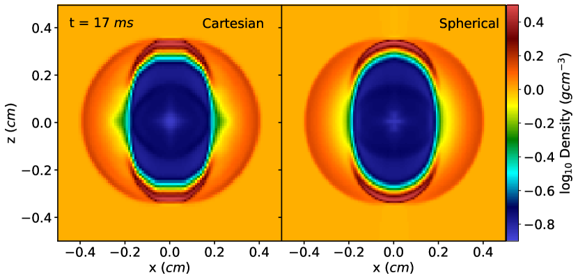
Figure 6: Density slice at 17 ms in $xz$-plane of the 3D-MHD blast wave in Cartesian (left) and spherical (right) coordinates. A slice along the $z$-direction is shown in Figure 7.

Both simulations produce the same overall expansion of the blast-wave, as shown in Figure 6. The only large quantitative difference occurs at the origin, where the reflecting inner radial boundary condition causes small differences in magnetic field evolution. In the cartesian explosion, the field is continuous across $x=0$ and not reflecting. In Athena++, Skinner & Ostriker (2010) perform an off-center explosion to remove this difference, but we choose not to do so here due to the large resolution requirements. Also, an off-center explosion does not take advantage of the symmetry of the coordinate system. The cartesian test also shows visible edges, which can be attributed to the shock being steeper in the spherical geometry.

Figure 7: Density slices along the $z-$direction ($x=0$, $y=0$) in the 3D MHD blast wave test, with geometries and times as labeled (see also Figure 6). Notable differences appear in the magnetic pressure throughout the entire evolution due to the difference in boundary conditions between the two simulations. Other differences can be attributed to the geometry and resolution.

We numerically compare a slice along the Cartesian $z-$direction in Figure 7. The two differences described previously are also noticeable in these plots, especially in the magnetic field at the inner boundary. However, both codes track the shock position identically, and the only noticeable differences appear at sharp gradients.

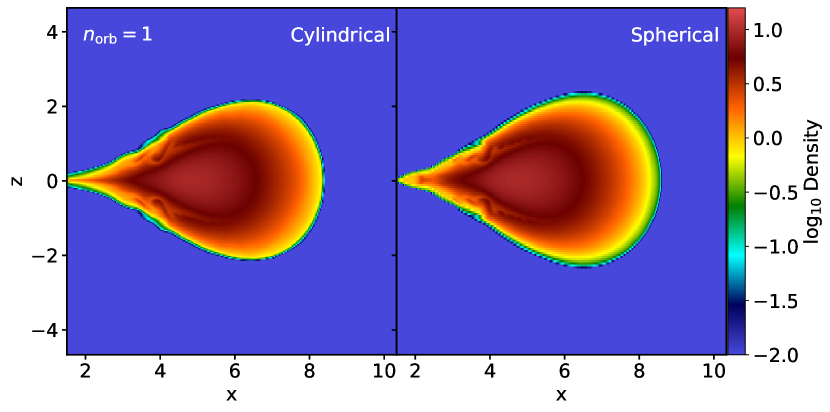
Figure 8: Density snapshot of the 2.5D axisymmetric torus test after one orbit at the initial density peak radius. The density field in cylindrical (left) and spherical (right) coordinates is normalized to code units, with a maximum value of 10. Noticeable differences appear in regions near the origin, where the flow is slightly more resolved in spherical coordinates.

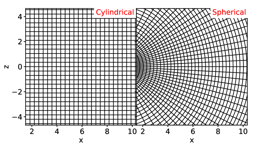
Figure 9: Comparison of the grid setup in cylindrical and spherical coordinates for the 2.5D torus test runs. Every 10^th grid line is plotted for visual clarity. The spherical grid is more resolved towards the inner radial part of the midplane, but at comparable resolutions in the rest of the torus. The outer polar regions are less resolved to reduce constraints on the simulation time step.

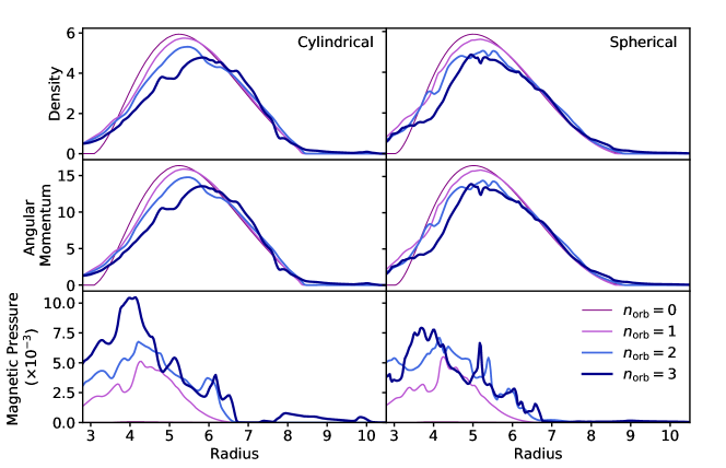
Figure 10: Results from the 2.5D axisymmetric torus tests, evolved for 3 orbits at the initial radius of maximum density $r_{\rm circ}$. The left column shows the height-averaged density, angular momentum, and magnetic pressure (all in code units) in the cylindrical simulation, while the right column shows the same quantities for the spherical case but angle-averaged instead. Lines of increasing thickness show the torus evolution from its initial to final state at each orbit ($n_{\rm orb}$). Numerical differences between the angle- and height-averaging appear even at the 0th orbit, but the general trends are not affected.

B.2 Magnetized Torus Results

We perform two torus tests. The first is carried out in 2.5D in both cylindrical and spherical coordinates, and employs a standard and normal evolution (SANE) initial magnetic field configuration. Results can be compared to multiple previous implementations (Hawley, 2000; Mignone et al., 2007; Tzeferacos et al., 2012). The second test is the extension to 3D spherical coordinates of the same SANE torus.

We set up the tori as in Fahlman (2019), using the gravitational potential of (Paczyńsky & Wiita, 1980) and setting the gravitating mass, $M=1$. We normalize units such that $G=c=1$. We choose the same parameters as model GT1 from Hawley (2000), which creates a thin, constant angular momentum torus with a maximum density of 10 and an orbital timescale of $\sim 50$ at the initial circularization radius $r_{\mathrm{circ}}=4.7$, and a minimum radius of $r=3$. The initial vector potential follows the density distribution,

$$A_{\phi}=\max(\rho-\frac{1}{2}\rho_{\mathrm{max}},0),$$ (50)

which creates poloidal field loops threaded well within the torus. Initially, the field is normalized to $\langle\beta\rangle=100$, so the field is dynamically unimportant and does not disturb the equilibrium condition The tori are then evolved for a total of $\sim 3$ orbits at $r_{\rm circ}$.

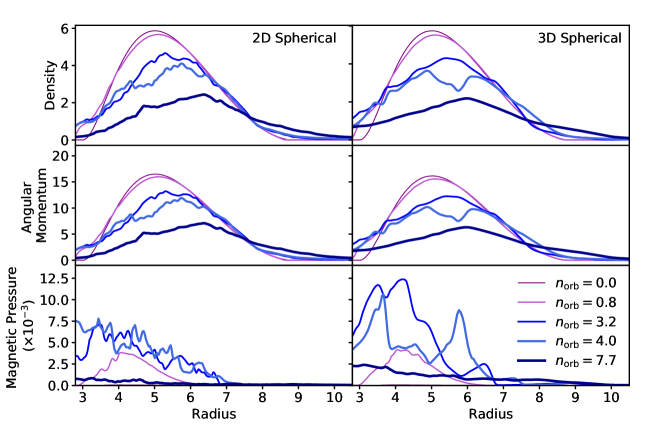
Figure 11: Comparison between the 2.5D axisymmetric and 3D torus test in spherical coordinates, showing the same angle-averaged quantities as in Figure 10 at various times. Both runs follow the expected evolution: the 3D torus sustains a more powerful MRI for a longer time due to the additional azimuthal turbulence, with the evolution being otherwise identical during the first $\sim$2 orbits. Differences in spatial resolution manifest as smoother profiles in the 3D runs, which has coarser cell sizes.

We compare the evolution of hydrodynamic variables in the 2.5D runs quantitatively and qualitatively in Figures (8-10). One notable difference between the two axisymmetric runs is the resolution and the inner boundary. In cylindrical coordinates, the entire inner $z-$boundary is set to be absorbing, while in spherical coordinates the inner radial boundary is set to be absorbing, and the polar boundaries are reflecting. This affects the dynamics near the inner edges of the torus, which is noticeable in the magnetic fields. The resolution in the two runs is comparable, but not exactly the same as necessitated by the difference in grid structures. The spherical run resolves the torus better, with $\Delta r=0.028$ and the highest angular resolution in the midplane, $r_{\mathrm{circ}}\min(\Delta\theta)=0.024$, resulting in nearly square cells at that location, compared to the constant cylindrical resolution of $\Delta r_{\mathrm{cyl}}=0.035$ and $\Delta z=0.035$. The two grids are shown in Figure 9 for reference.

The axisymmetric runs follow the same qualitative evolution in cylindrical and spherical coordinates: the azimuthal magnetic field grows due to winding, and the magnetic pressure causes the torus to expand and accrete. The radial angular momentum profile flattens as matter approaches the ISCO, and the magnetic field grows largest in the central regions and then accretes, frozen in with the mass flow. The first large divergences between the two simulations begin to appear in the magnetic field after $\sim 1$ orbit at $r_{\rm circ}$, when the accretion stream reaches the inner boundary. Feedback from the reflecting boundary changes the expansion of the torus into the ambient between the two cases. Furthermore, additional turbulent structures manifest in the spherical torus, noticeable as less smooth profiles in Figure 10. We attribute this in part to the differences in spatial resolution, and also note that Mignone et al. (2007) see similar effects in their PLUTO code tests with spherical and cylindrical coordinates and the exact same setup (see their Figure 8).

The 3D SANE torus follows the same evolution as the axisymmetric spherical case for the first few orbits, as shown in Figure 11. Notable differences begin to appear after $\sim$3 orbits at $r_{\rm circ}$, as the MRI begins to die down in the axisymmetric run. In 3D, the MRI creates stronger magnetic fields and is sustained for longer through the additional turbulence in the azimuthal direction (Hawley, 2000). The profiles in the 3D run appear smoother, as we run it with a lower resolution than in the 2D case due to computational limitations. To make up for this difference in resolution, we use a logarithmic grid in radius in the 3D model, so that the region containing the torus is still resolved well. This corresponds to resolutions in the radial, polar, and azimuthal directions being $\Delta r_{\mathrm{circ}}\sim 0.040$, $r_{\mathrm{circ}}\min(\Delta\theta)=0.10$, and $\Delta\phi=0.03$.

Appendix C Neutrino Leakage Scheme

Neutrinos change the composition of disk outflows through charged current weak interactions that alter the ratio of protons to neutrons. These transformations proceed via emission or absorption of electron neutrinos and antineutrinos. A common approach to modeling emission of neutrinos is the so-called “leakage scheme” (Ruffert et al., 1996), which interpolates between the diffusive and transparent regimes of radiative transport. Leakage schemes have been shown to capture the dominant effects of neutrinos in post-merger tori around compact objects, especially for BH disks, for which they are subdominant energy sources (Foucart et al., 2019; Fernández & Metzger, 2013; Siegel & Metzger, 2018; Fernández et al., 2019a). However, significant differences appear when compared quantitatively to more advanced Monte-Carlo or two-moment (M1) schemes (Richers et al., 2015; Foucart et al., 2015; Perego et al., 2016; Ardevol-Pulpillo et al., 2019; Radice et al., 2021). For this reason it is necessary to make impovements to the previous leakage-scheme implemented in FLASH (Fernández & Metzger, 2013; Metzger & Fernández, 2014), while retaining computational efficiency.

C.1 Leakage Overview

The key components of a leakage scheme are the two source terms that describe the effective neutrino energy and number loss rate per unit volume for each neutrino species,

$${Q}^{\rm eff}_{\nu_{i}}=Q_{\nu_{i}}\chi_{{\nu_{i}},E},$$ (51)

$${R}^{\rm eff}_{\nu_{i}}=R_{\nu_{i}}\chi_{{\nu_{i}},N},$$ (52)

where $i$ represents a species ($\nu_{e}$ or $\bar{\nu}_{e}$ in our scheme), the subscripts $E$ and $N$ refer to energy and number, respectively. $Q$ and $R$ are the energy and number production rates per unit volume, respectively, which are obtained from analytic expressions (Ruffert et al., 1996). The scaling factors $\chi_{{\nu_{i}},E}$ and $\chi_{{\nu_{i}},N}$ interpolate between the free-streaming and optically thick (diffusive) regimes for neutrinos in both energy and number,

$$\chi_{{\nu_{i}},\{E,N\}}=\bigg{(}1+\frac{t^{\mathrm{diff}}_{{\nu_{i}},\{E,N\}}}{t^{\mathrm{loss}}_{{\nu_{i}},\{E,N\}}}\bigg{)}^{-1},$$ (53)

where $t^{\mathrm{diff}}_{\nu_{i}}$ and $t^{\mathrm{loss}}_{\nu_{i}}$ are the diffusion and loss timescales for each species, respectively. The source terms for equations (3)-(4) are then obtained as follows

$$Q_{\rm net} = Q^{\rm eff}_{\nu_{e}}+Q^{\rm eff}_{\bar{\nu}_{e}}+Q_{\rm abs}$$ (54)

$$\Gamma_{\rm net} = \frac{m_{n}}{\rho}\left(R^{\rm eff}_{\nu_{e}}+R^{\rm eff}_{\bar{\nu}_{e}}\right)+\Gamma_{\rm abs},$$ (55)

where $Q_{\rm abs}$ and $\Gamma_{\rm abs}$ are the contributions from neutrino absorption (treated separately) and $m_{n}$ is the neutron mass. The diffusion and loss timescales in equation (53) are central to the accuracy of the scheme, and thus we will discuss them in more detail.

C.1.1 Loss timescale

Once the direct energy and number production rates in (51-52) are found, the loss times are obtained as

$$t^{\mathrm{loss}}_{{\nu_{i}},E}=\frac{Q_{\nu_{i}}}{E_{\nu_{i}}}$$ (56)

$$t^{\mathrm{loss}}_{{\nu_{i}},N}=\frac{R_{\nu_{i}}}{N_{\nu_{i}}},$$ (57)

where $E_{\nu_{i}}$ and $N_{\nu_{i}}$ are the neutrino energy density and number density, respectively. These quantities are obtained using analytic fits to Fermi integrals from Takahashi et al. (1978).

Figure 12: Outflow mass histogram as a function of electron fraction after 1 s of evolution from two axisymmetric hydrodynamic BH disk setups that employ the old and new implementation of diffusion time in the neutrino leakage scheme (equations 58-59 and 63 from Ardevol-Pulpillo et al. 2019, respectively). The average electron fraction of the outflow increases by 5%, and the outflow quantity decreases by about $50\%$ in the new scheme, as the diffusion time correspondingly decreases by an order of magnitude. This difference in outflow properties comes from the high velocity neutrino-driven, early time outflows, which retain less energy deposited by neutrinos, since cooling is more efficient.

C.1.2 Diffusion timescale

The diffusion timescale is approximately given by

$$t^{\mathrm{diff}}_{{\nu_{i}},\{E,N\}}\sim\frac{3\kappa_{{\nu_{i}},\{E,N\}}d^{2}}{c}.$$ (58)

where $\kappa_{{\nu_{i}},\{E,N\}}$ is the energy or number opacity for species $i$, and $d$ is a characteristic diffusion distance. A more accurate expression involves calculation of the optical depth in various directions, which many leakage schemes incorporate (e.g., Rosswog & Liebendörfer 2003), but which is a global calculation that is computationally expensive. Our previous leakage implementation (Fernández & Metzger, 2013; Metzger & Fernández, 2014) approximates $d$ as the pressure scale height assuming hydrostatic equilibrium in the cylindrical z-direction, which is the preferential direction for neutrinos to escape the torus,

$$d\approx\frac{P}{\big{(}\frac{\partial P}{\partial r}\big{)}}=\frac{P}{\rho|\cos\theta g|}.$$ (59)

This is a local calculation which yields a neutrino optical depth correct to within a factor of $\sim 2$.

Recently, Ardevol-Pulpillo et al. (2019) have developed a novel method for determining the diffusion timescale which is local (computationally efficient) and accurate. In this method, the diffusion timescale is determined from the diffusion equation using a flux limiter

$$\frac{\partial\{E,N\}_{\nu_{i}}}{\partial t}=-\vec{\nabla}\cdot{\mathbf{F}_{{\nu_{i}},\{E,N\}}}$$ (60)

where $\mathbf{F}_{{\nu_{i}},\{E,N\}}$ is the neutrino energy of number flux, respectively. In flux-limited diffusion (FLD, see e.g., Wilson et al., 1975; Levermore & Pomraning, 1981; Kolb et al., 2013), the flux is given by

$$\mathbf{F}_{{\nu_{i}},\{E,N\}}=-\frac{c}{3\kappa_{\nu_{i}}}\Lambda_{{\nu_{i}},\{E,N\}}\nabla\{E,N\}_{\nu_{i}},$$ (61)

where $\Lambda_{{\nu_{i}},\{E,N\}}$ is a flux limiter that interpolates between pure diffusion ($\Lambda_{{\nu_{i}},\{E,N\}}=1$) and free-streaming (${F}_{{\nu_{i}},\{E,N\}}=c\{E_{\nu_{i}},N_{\nu_{i}}\}$). The diffusion times can be determined analogously to the loss timescales:

$$t^{\mathrm{diff}}_{{\nu_{i}},\{E,N\}}=\frac{\{E,N\}_{\nu_{i}}}{\bigg{(}\dfrac{\partial\{E,N\}_{\nu_{i}}}{\partial t}\bigg{)}}.$$ (62)

Expanding out the time derivative using the diffusion equations (61) and energy/number transport (60) yields

$$t^{\mathrm{diff}}_{{\nu_{i}},\{E,N\}}=\frac{\{E,N\}_{\nu_{i}}}{\vec{\nabla}\cdot{(\frac{-c}{3\kappa_{\nu_{i}}}\Lambda_{{\nu_{i}},\{E,N\}}\nabla\{E,N\}_{\nu_{i}}})}.$$ (63)

We follow Ardevol-Pulpillo et al. (2019) in using the flux limiter of Wilson et al. (1975) for each species,

$$\Lambda_{{\nu_{i}},\{E,N\}}=\bigg{(}1+\frac{1}{3\kappa_{\nu_{i}}}\frac{|\nabla\{E,N\}_{\nu_{i}}|}{\{E,N\}_{\nu_{i}}}\bigg{)}^{-1},$$ (64)

In contrast to Ardevol-Pulpillo et al. (2019) who integrate quantities over the neutrino distribution, we use energy-averaged (over a Fermi-Dirac distribution) opacities, energy densities, and number densities in equation (63), computing only the spatial gradient.

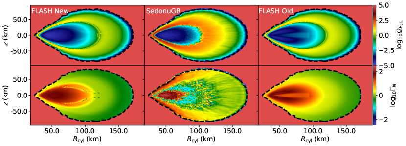
Figure 13: Comparison of neutrino source terms (Top: energy rate per unit mass in cgs, Bottom: number rate per baryon) obtained using a leakage scheme with the diffusion time prescription from Ardevol-Pulpillo et al. (2019) and light bulb absorption (Left: FLASH New), Center: SedonuGR Monte-Carlo transport, and the leakage scheme plus light bulb absorption previously implemented in Metzger & Fernández (2014) (Right: FLASH Old). The background fluid quantities correspond to a snapshot of the FLASH New simulation at $0.6\,\mathrm{ms}$ The new leakage scheme no longer artificially suppresses the source terms in the midplane of the torus, coming closer to the results of SedonuGR. Contours of $10^{5}$g cm^-3 in density are shown as thick dashed lines, corresponding to the density cutoff at which SedonuGR no longer performs neutrino calculations.

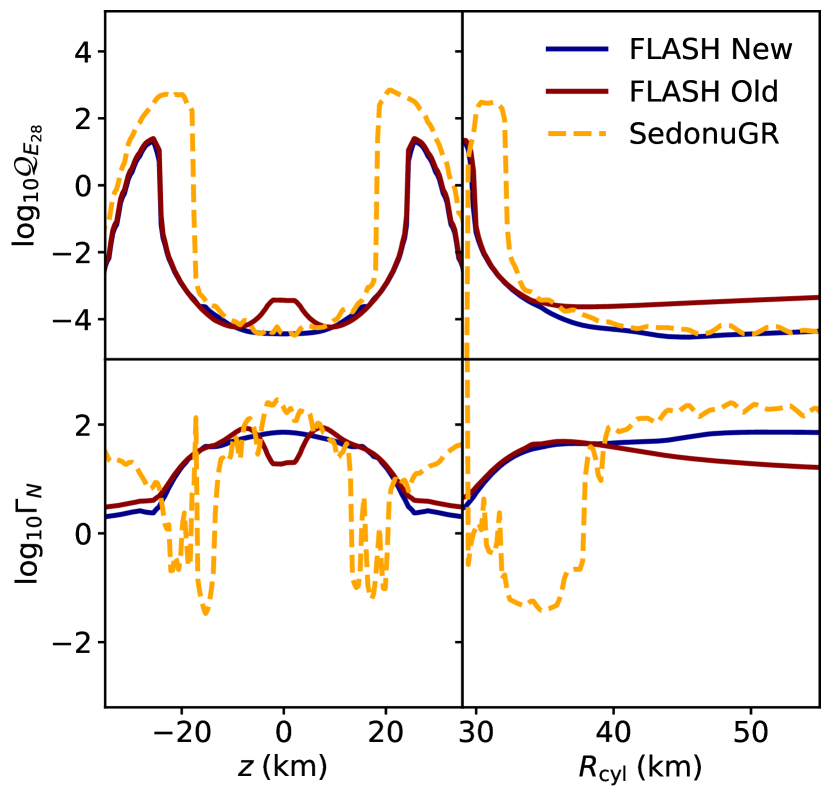
Figure 14: Comparison of neutrino source terms in the updated leakage scheme (FLASH New), SedonuGR, and the leakage scheme previously implemented (FLASH Old). Like in Figure 13, the top rows show rate of change of internal energy, but this time taking a slice through the density maximum in the $z$-direction (left), and a slice through the equatorial plane (right) of the $0.03M_{\odot}$ torus at $0.6\,\mathrm{ms}$. The bottom panels are identical slices but for the rate of change of lepton number. The leakage schemes follow approximately the correct curve, as previously shown (Richers et al., 2015), but once again the new scheme is closer to the MC method of SedonuGR, particularly when it comes to the source terms in the torus midplane.

Figure 15: Same as Figure 13, but for a $0.1M_{\odot}$ torus evolved with 2D-MHD at $\sim 30\,\mathrm{ms}$ using the updated leakage scheme and comparing with SedonuGR. There are no previous MHD results to compare with. Overall, SedonuGR and the new leakage scheme show similar trends in both heating/cooling and change in lepton number. SedonuGR does not discriminate between ambient and torus material, while our scheme does not perform neutrino calculations on ambient matter. This appears as purple areas in the poloidal regions of the FLASH simulations.

Figure 16: Same as Figure 14, but for a $0.1M_{\odot}$ torus evolved with 2D-MHD and the updated leakage scheme at $\sim 30$ ms. There are no previous MHD results to compare with, but the overall effects of neutrinos are captured well, with significant deviations only in small localized regions.

C.2 Implementation in FLASH4.5

We extend the leakage and light bulb absorption scheme of Fernández & Metzger (2013) and Metzger & Fernández (2014) by computing the diffusion time with equation (63) and implement it in FLASH4.5. Neutrino energy and number gradients are obtained using second order finite differences in each spatial direction, The flux limiters are calculated for each species as in (64). The flux limiters are then combined with the gradients, energy/number densities, and opacities to form the fluxes in 61. The fluxes are then linearly interpolated to the cell faces, such that we can take a numerical divergence using Gauss’s theorem (26) and the face areas of a given cell, analogous to the unsplit update in §A.1.

C.2.1 Comparison with 2D hydrodynamic simulations

We test the effect of the new diffusion time on the long-term disk evolution by running a 2D axisymmetric hydrodynamic simulation of an accretion torus using the previous leakage scheme and the new one. A full description of the methodology is available in Fernández & Metzger (2013); Metzger & Fernández (2014), here we briefly describe the initial setup. The compact object is a BH with mass $3M_{\odot}$, and the orbiting equilibrium torus is chosen to be optically thin with a mass of $0.03M_{\odot}$. The entropy, electron fraction, and torus distortion parameter are chosen to be $8k_{B}/\mathrm{baryon}$, $0.1$, and $1.911$, respectively. This yields a well-studied initial condition compatible with dynamical merger simulations (Fernández & Metzger, 2013; Metzger & Fernández, 2014; Richers et al., 2015; Lippuner et al., 2017). Angular momentum transport is handled with the viscous stress parameterization of Shakura & Sunyaev (1973), with $\alpha$ set to $0.05$. The tori are evolved for 1 second.

The average mass-flux-weighted electron fraction of the outflow increases by $5\%$ when using the new diffusion time formulation, as shown in the histogram of torus outflows in Figure 12. This result corresponds to a decrease in diffusion time by a factor of $\sim 10$ in the high-density regions of the torus. Neutrinos are still preferentially trapped near the midplane, but the new methodology no longer overestimates this effect for the optically thin torus. The new method yields about 50% less mass outflows, predominately due to the same effect: the energy deposited into early time outflows is cooled more efficiently, unbinding less material. The major difference occurs in the neutrino-driven outflow ejected from the back of the torus, with electron fraction $Y_{e}\sim 0.25$. We caution that this difference will likely not extend to the late-time, radiatively inefficient evolution, as the energy and density of late time outflows appear identical, and affects mainly the initial winds.

C.2.2 Comparison with SedonuGR in Hydro

We compare the emission and absorption of neutrinos to the Monte-Carlo neutrino transport code SedonuGR (Richers et al., 2015, 2017). We are interested in the rate of change of lepton number, which governs the change in electron fraction, and the rate of change of internal energy, which governs changes in internal energy of the ejecta due to neutrinos. Following Richers et al. (2015), we load a fluid snapshot from the FLASH4.5 simulation using the new method in SedonuGR. We use the Helmholtz EOS in SedonuGR for consistency.

At late times, the neutrino scheme for the optically thin torus shows minimal differences with the full Monte-Carlo results (Richers et al., 2015). The changes to the neutrino scheme are most evident at very early times, so we choose a time of $\sim$0.6 ms for the comparison, the result of which is shown in Figure 13. Most of the differences in source terms occur in the regions where absorption becomes important, which in our approach is handled by an approximate light bulb implementation (Fernández & Metzger, 2013; Metzger & Fernández, 2014), which we did not modify here. Importantly, the new neutrino leakage scheme no longer suppresses neutrino emission in the midplane of the torus, where the pressure scale height is comparatively large. This is shown quantitatively with slices in the equatorial plane and along the $z$-direction at the torus density maximum in Figure 14.

C.2.3 MHD Comparison with SedonuGR

Since our base torus is more massive than those used in the previous hydrodynamic test runs, and MHD evolution differs in comparison to viscous hydrodynamics, we also show a comparison of our leakage scheme in 2D-MHD with results from SedonuGR (Figure 15). Equatorial and vertical slices through the density maximum of a torus identical to our base model are shown in Figure 16 at 30 ms, when the neutrinos are important for setting the electron fraction of the outflows. Importantly, the source term modifying the electron fraction remains of the same order of magnitude across most of the torus.

References

- Abbott et al. (2017a) Abbott B. P., et al., 2017a, PRL, 119, 161101
- Abbott et al. (2017b) Abbott B. P., et al., 2017b, ApJ, 848, L12
- Abbott et al. (2017c) Abbott B. P., et al., 2017c, ApJ, 848, L13
- Abbott et al. (2021) Abbott R., Abbott T. D., Abraham S., et al., 2021, Physical Review X, 11, 021053
- Ardevol-Pulpillo et al. (2019) Ardevol-Pulpillo R., Janka H. T., Just O., Bauswein A., 2019, MNRAS, 485, 4754
- Artemova et al. (1996) Artemova I. V., Bjoernsson G., Novikov I. D., 1996, ApJ, 461, 565
- Balbus & Hawley (1991) Balbus S. A., Hawley J. F., 1991, ApJ, 376, 214
- Balbus & Hawley (1992) Balbus S. A., Hawley J. F., 1992, ApJ, 400, 610
- Bardeen & Petterson (1975) Bardeen J. M., Petterson J. A., 1975, ApJ, 195, L65
- Barnes & Kasen (2013) Barnes J., Kasen D., 2013, ApJ, 775, 18
- Blandford & Znajek (1977) Blandford R. D., Znajek R. L., 1977, MNRAS, 179, 433
- Childs et al. (2012) Childs H., et al., 2012, in , High Performance Visualization–Enabling Extreme-Scale Scientific Insight. eScholarship, University of California, pp 357–372
- Chornock et al. (2017) Chornock R., et al., 2017, ApJ, 848, L19
- Christie et al. (2019) Christie I. M., Lalakos A., Tchekhovskoy A., Fernández R., Foucart F., Quataert E., Kasen D., 2019, MNRAS, 490, 4811
- Ciolfi & Kalinani (2020) Ciolfi R., Kalinani J. V., 2020, ApJ, 900, L35
- Colella (1985) Colella P., 1985, SIAM Journal on Scientific and Statistical Computing, 6, 104
- Cowling (1933) Cowling T. G., 1933, MNRAS, 94, 39
- Cowperthwaite et al. (2017) Cowperthwaite P. S., et al., 2017, ApJ, 848, L17
- Curtis et al. (2021) Curtis S., Mösta P., Wu Z., Radice D., Roberts L., Ricigliano G., Perego A., 2021, preprint, p. arXiv:2112.00772
- De Villiers et al. (2005) De Villiers J.-P., Hawley J. F., Krolik J. H., Hirose S., 2005, ApJ, 620, 878
- Drout et al. (2017) Drout M. R., et al., 2017, Science, 358, 1570
- Dubey et al. (2009) Dubey A., Antypas K., Ganapathy M. K., Reid L. B., Riley K., Sheeler D., Siegel A., Weide K., 2009, Parallel Computing, 35, 512
- Duez et al. (2006) Duez M. D., Liu Y. T., Shapiro S. L., Shibata M., Stephens B. C., 2006, Phys. Rev. Lett., 96, 031101
- Eichler et al. (1989) Eichler D., Livio M., Piran T., Schramm D. N., 1989, Nature, 340, 126
- Evans & Hawley (1988) Evans C. R., Hawley J. F., 1988, ApJ, 332, 659
- Fahlman (2019) Fahlman S., 2019, Master’s thesis, University of Alberta, doi:10.7939/r3-6877-8m55
- Fahlman & Fernández (2018) Fahlman S., Fernández R., 2018, ApJ, 869, L3
- Fernández & Metzger (2013) Fernández R., Metzger B. D., 2013, MNRAS, 435, 502
- Fernández et al. (2015) Fernández R., Kasen D., Metzger B. D., Quataert E., 2015, MNRAS, 446, 750
- Fernández et al. (2019a) Fernández R., Tchekhovskoy A., Quataert E., Foucart F., Kasen D., 2019a, MNRAS, 482, 3373
- Fernández et al. (2019b) Fernández R., Margalit B., Metzger B. D., 2019b, MNRAS, 488, 259
- Fernández et al. (2020) Fernández R., Foucart F., Lippuner J., 2020, MNRAS, 497, 3221
- Foley et al. (2020) Foley R. J., Coulter D. A., Kilpatrick C. D., Piro A. L., Ramirez-Ruiz E., Schwab J., 2020, MNRAS, 494, 190
- Fontes et al. (2015) Fontes C. J., Fryer C. L., Hungerford A. L., Hakel P., Colgan J., Kilcrease D. P., Sherrill M. E., 2015, High Energy Density Physics, 16, 53
- Foucart et al. (2015) Foucart F., et al., 2015, Phys. Rev. D, 91, 124021
- Foucart et al. (2019) Foucart F., Duez M. D., Kidder L. E., Nissanke S. M., Pfeiffer H. P., Scheel M. A., 2019, Phys. Rev. D, 99, 103025
- Foucart et al. (2020) Foucart F., Duez M. D., Hebert F., Kidder L. E., Pfeiffer H. P., Scheel M. A., 2020, ApJ, 902, L27
- Fryxell et al. (2000) Fryxell B., et al., 2000, ApJS, 131, 273
- Fujibayashi et al. (2018) Fujibayashi S., Kiuchi K., Nishimura N., Sekiguchi Y., Shibata M., 2018, ApJ, 860, 64
- Fujibayashi et al. (2020a) Fujibayashi S., Shibata M., Wanajo S., Kiuchi K., Kyutoku K., Sekiguchi Y., 2020a, Phys. Rev. D, 102, 123014
- Fujibayashi et al. (2020b) Fujibayashi S., Wanajo S., Kiuchi K., Kyutoku K., Sekiguchi Y., Shibata M., 2020b, ApJ, 901, 122
- Gottlieb et al. (2018) Gottlieb O., Nakar E., Piran T., 2018, MNRAS, 473, 576
- Hawley (2000) Hawley J. F., 2000, ApJ, 528, 462
- Hawley & Krolik (2001) Hawley J. F., Krolik J. H., 2001, ApJ, 548, 348
- Hawley & Krolik (2006) Hawley J. F., Krolik J. H., 2006, ApJ, 641, 103
- Hayashi et al. (2021) Hayashi K., Fujibayashi S., Kiuchi K., Kyutoku K., Sekiguchi Y., Shibata M., 2021, arXiv e-prints, p. arXiv:2111.04621
- Heinzel et al. (2021) Heinzel J., et al., 2021, MNRAS, 502, 3057
- Hossein Nouri et al. (2018) Hossein Nouri F., et al., 2018, Phys. Rev. D, 97, 083014
- Janiuk (2017) Janiuk A., 2017, ApJ, 837, 39
- Janiuk et al. (2013) Janiuk A., Mioduszewski P., Moscibrodzka M., 2013, ApJ, 776, 105
- Just et al. (2015) Just O., Bauswein A., Ardevol Pulpillo R., Goriely S., Janka H.-T., 2015, MNRAS, 448, 541
- Just et al. (2022) Just O., Goriely S., Janka H. T., Nagataki S., Bauswein A., 2022, MNRAS, 509, 1377
- Kasen et al. (2013) Kasen D., Badnell N. R., Barnes J., 2013, ApJ, 774, 25
- Kasen et al. (2015) Kasen D., Fernández R., Metzger B. D., 2015, MNRAS, 450, 1777
- Kasen et al. (2017) Kasen D., Metzger B., Barnes J., Quataert E., Ramirez-Ruiz E., 2017, Nature, 551, 80
- Kawaguchi et al. (2020) Kawaguchi K., Shibata M., Tanaka M., 2020, ApJ, 889, 171
- Kawaguchi et al. (2021) Kawaguchi K., Fujibayashi S., Shibata M., Tanaka M., Wanajo S., 2021, ApJ, 913, 100
- Kiuchi et al. (2012) Kiuchi K., Kyutoku K., Shibata M., 2012, PRD, 86, 064008
- Klion et al. (2022) Klion H., Tchekhovskoy A., Kasen D., Kathirgamaraju A., Quataert E., Fernández R., 2022, MNRAS, 510, 2968
- Kolb et al. (2013) Kolb S. M., Stute M., Kley W., Mignone A., 2013, A&A, 559, A80
- Komissarov (1999) Komissarov S. S., 1999, MNRAS, 303, 343
- Korobkin et al. (2021) Korobkin O., et al., 2021, ApJ, 910, 116
- Krüger & Foucart (2020) Krüger C. J., Foucart F., 2020, Phys. Rev. D, 101, 103002
- Kuroda et al. (2020) Kuroda T., Arcones A., Takiwaki T., Kotake K., 2020, ApJ, 896, 102
- Lattimer & Schramm (1974) Lattimer J. M., Schramm D. N., 1974, The Astrophysical Journal, 192, L145
- Lee (2013) Lee D., 2013, Journal of Computational Physics, 243, 269
- Lee & Deane (2009) Lee D., Deane A. E., 2009, Journal of Computational Physics, 228, 952
- Levermore & Pomraning (1981) Levermore C. D., Pomraning G. C., 1981, ApJ, 248, 321
- Li & Paczyński (1998) Li L.-X., Paczyński B., 1998, ApJ, 507, L59
- Lippuner & Roberts (2015) Lippuner J., Roberts L. F., 2015, ApJ, 815, 82
- Lippuner et al. (2017) Lippuner J., Fernández R., Roberts L. F., Foucart F., Kasen D., Metzger B. D., Ott C. D., 2017, MNRAS, 472, 904
- Loken et al. (2010) Loken C., et al., 2010, in Journal of Physics Conference Series. p. 012026, doi:10.1088/1742-6596/256/1/012026
- Margalit & Metzger (2016) Margalit B., Metzger B. D., 2016, MNRAS, 461, 1154
- Metzger & Fernández (2014) Metzger B. D., Fernández R., 2014, MNRAS, 441, 3444
- Metzger et al. (2009) Metzger B. D., Piro A. L., Quataert E., 2009, MNRAS, 396, 304
- Metzger et al. (2010) Metzger B. D., et al., 2010, MNRAS, 406, 2650
- Metzger et al. (2018) Metzger B. D., Thompson T. A., Quataert E., 2018, ApJ, 856, 101
- Mignone & Del Zanna (2021) Mignone A., Del Zanna L., 2021, Journal of Computational Physics, 424, 109748
- Mignone et al. (2005) Mignone A., Plewa T., Bodo G., 2005, ApJS, 160, 199
- Mignone et al. (2007) Mignone A., Bodo G., Massaglia S., Matsakos T., Tesileanu O., Zanni C., Ferrari A., 2007, ApJS, 170, 228
- Miller et al. (2019) Miller J. M., et al., 2019, Phys. Rev. D, 100, 023008
- Miyoshi & Kusano (2005) Miyoshi T., Kusano K., 2005, Journal of Computational Physics, 208, 315
- Most et al. (2019) Most E. R., Papenfort L. J., Tsokaros A., Rezzolla L., 2019, ApJ, 884, 40
- Most et al. (2021) Most E. R., Papenfort L. J., Tootle S. D., Rezzolla L., 2021, MNRAS, 506, 3511
- Mösta et al. (2020) Mösta P., Radice D., Haas R., Schnetter E., Bernuzzi S., 2020, ApJ, 901, L37
- Murguia-Berthier et al. (2021) Murguia-Berthier A., Noble S. C., Roberts L. F., et al., 2021, ApJ, 919, 95
- Nedora et al. (2020) Nedora V., et al., 2020, arXiv e-prints, p. arXiv:2011.11110
- Paczynski (1986) Paczynski B., 1986, ApJ, 308, L43
- Paczyńsky & Wiita (1980) Paczyńsky B., Wiita P. J., 1980, A&A, 500, 203
- Perego et al. (2014) Perego A., Rosswog S., Cabezón R. M., Korobkin O., Käppeli R., Arcones A., Liebendörfer M., 2014, MNRAS, 443, 3134
- Perego et al. (2016) Perego A., Cabezón R. M., Käppeli R., 2016, ApJS, 223, 22
- Piro & Kollmeier (2018) Piro A. L., Kollmeier J. A., 2018, ApJ, 855, 103
- Ponce et al. (2019) Ponce M., et al., 2019, arXiv e-prints, p. arXiv:1907.13600
- Raaijmakers et al. (2021) Raaijmakers G., et al., 2021, ApJ, 922, 269
- Radice et al. (2018) Radice D., Perego A., Hotokezaka K., Fromm S. A., Bernuzzi S., Roberts L. F., 2018, The Astrophysical Journal, 869, 130
- Radice et al. (2021) Radice D., Bernuzzi S., Perego A., Haas R., 2021, arXiv e-prints, p. arXiv:2111.14858
- Richers et al. (2015) Richers S., Kasen D., O’Connor E., Fernández R., Ott C. D., 2015, ApJ, 813, 38
- Richers et al. (2017) Richers S., Nagakura H., Ott C. D., Dolence J., Sumiyoshi K., Yamada S., 2017, ApJ, 847, 133
- Rosswog & Liebendörfer (2003) Rosswog S., Liebendörfer M., 2003, MNRAS, 342, 673
- Ruffert et al. (1996) Ruffert M., Janka H. T., Schaefer G., 1996, A&A, 311, 532
- Ruffert et al. (1997) Ruffert M., Janka H.-T., Takahashi K., Schaefer G., 1997, A&A, 319, 122
- Shakura & Sunyaev (1973) Shakura N. I., Sunyaev R. A., 1973, A&A, 24, 337
- Shibata & Sekiguchi (2012) Shibata M., Sekiguchi Y., 2012, Progress of Theoretical Physics, 127, 535
- Shibata et al. (2007) Shibata M., Sekiguchi Y.-I., Takahashi R., 2007, Progress of Theoretical Physics, 118, 257
- Shibata et al. (2017) Shibata M., Fujibayashi S., Hotokezaka K., Kiuchi K., Kyutoku K., Sekiguchi Y., Tanaka M., 2017, Phys. Rev. D, 96, 123012
- Shibata et al. (2021a) Shibata M., Fujibayashi S., Sekiguchi Y., 2021a, arXiv e-prints, p. arXiv:2102.01346
- Shibata et al. (2021b) Shibata M., Fujibayashi S., Sekiguchi Y., 2021b, Phys. Rev. D, 104, 063026
- Siegel & Metzger (2017) Siegel D. M., Metzger B. D., 2017, Physical Review Letters, 119, 231102
- Siegel & Metzger (2018) Siegel D. M., Metzger B. D., 2018, ApJ, 858, 52
- Siegel et al. (2014) Siegel D. M., Ciolfi R., Rezzolla L., 2014, ApJ, 785, L6
- Skinner & Ostriker (2010) Skinner M. A., Ostriker E. C., 2010, ApJS, 188, 290
- Takahashi et al. (1978) Takahashi K., El Eid M. F., Hillebrandt W., 1978, A&A, 67, 185
- Tanaka & Hotokezaka (2013) Tanaka M., Hotokezaka K., 2013, ApJ, 775, 113
- Tanaka et al. (2017) Tanaka M., et al., 2017, PASJ, 69, 102
- Tanvir et al. (2017) Tanvir N. R., et al., 2017, ApJ, 848, L27
- Tchekhovskoy et al. (2011) Tchekhovskoy A., Narayan R., McKinney J. C., 2011, MNRAS, 418, L79
- The LIGO Scientific Collaboration et al. (2021) The LIGO Scientific Collaboration the Virgo Collaboration the KAGRA Collaboration et al., 2021, PRX, submitted, p. arXiv:2111.03606
- Timmes & Swesty (2000) Timmes F. X., Swesty F. D., 2000, ApJS, 126, 501
- Tóth (2000) Tóth G., 2000, Journal of Computational Physics, 161, 605
- Tzeferacos et al. (2012) Tzeferacos P., et al., 2012, High Energy Density Physics, 8, 322
- Villar et al. (2017) Villar V. A., et al., 2017, ApJ, 851, L21
- Waxman et al. (2018) Waxman E., Ofek E. O., Kushnir D., Gal-Yam A., 2018, MNRAS, 481, 3423
- White et al. (2016) White C. J., Stone J. M., Gammie C. F., 2016, ApJS, 225, 22
- Wilson et al. (1975) Wilson J. R., Couch R., Cochran S., Le Blanc J., Barkat Z., 1975, in Bergman P. G., Fenyves E. J., Motz L., eds, Vol. 262, Seventh Texas Symposium on Relativistic Astrophysics. pp 54–64, doi:10.1111/j.1749-6632.1975.tb31420.x