Coupling Metric-Affine Gravity
to a Higgs-Like Scalar Field

Abstract

General Relativity (GR) exists in different formulations. They are equivalent in pure gravity but generically lead to distinct predictions once matter is included. After a brief overview of various versions of GR, we focus on metric-affine gravity, which avoids any assumption about the vanishing of curvature, torsion or non-metricity. We use it to construct an action of a scalar field coupled non-minimally to gravity. It encompasses as special cases numerous previously studied models. Eliminating non-propagating degrees of freedom, we derive an equivalent theory in the metric formulation of GR. Finally, we give a brief outlook to implications for Higgs inflation.

1 Introduction

1.1 The ambiguities of General Relativity

Einstein’s theory of General Relativity (GR) describes gravity in terms of the geometry of spacetime. In its original version Einstein:1915 , it is solely based on curvature – the rotation of vectors along closed curves. Correspondingly, the metric $g_{\mu\nu}$ is the unique fundamental variable, i.e., there are only equations of motion for $g_{\mu\nu}$. The affine connection is determined a priori as a function of $g_{\mu\nu}$. Its Christoffel symbols are defined by the conditions $\mathring{\Gamma}^{\alpha}_{~{}~{}\beta\gamma}=\mathring{\Gamma}^{\alpha}_{~{}~{}\gamma\beta}$ and $\mathring{\nabla}_{\alpha}g_{\mu\nu}=0$, which leads to the unique Levi-Civita connection. One can call this approach the metric formulation of GR.

It was soon realized that there is another possibility: One can treat the metric $g_{\mu\nu}$ and the Christoffel symbols $\Gamma^{\alpha}_{~{}~{}\beta\gamma}$ as independent and regard both of them as fundamental variables Weyl:1918 ; Palatini:1919 ; Weyl:1922 ; Eddington:1923 ; Cartan:1922 ; Cartan:1923 ; Cartan:1924 ; Cartan:1925 ; Einstein:1925 ; Einstein:1928 ; Einstein:19282 . In this case, the Christoffel symbols $\Gamma^{\alpha}_{~{}~{}\beta\gamma}$ can deviate from the Levi-Civita connection $\mathring{\Gamma}^{\alpha}_{~{}~{}\beta\gamma}$ and are determined by their own equations of motions. This leads to the emergence of two additional geometrical concepts. The first one, proposed by Cartan Cartan:1922 ; Cartan:1923 ; Cartan:1924 ; Cartan:1925 , is torsion $T^{\alpha}_{~{}~{}\beta\gamma}\propto\Gamma^{\alpha}_{~{}~{}\beta\gamma}-\Gamma^{\alpha}_{~{}~{}\gamma\beta}$, which corresponds to the non-closure of infinitesimal parallelograms. The second one was put forward by Weyl Weyl:1918 ; Weyl:1922 and consists in non-metricity $Q_{\alpha\mu\nu}\propto\nabla_{\alpha}g_{\mu\nu}$. It causes the non-conservation of vector norms in parallel transport.

The metric formulation of GR is based on the assumption that both torsion and non-metricity vanish, i.e., that gravity is solely characterized by the curvature of spacetime. It is possible, however, to relax these conditions. Already in 1918, Weyl proposed a theory that features non-metricity in addition to curvature Weyl:1918 (see also Weyl:1922 ; Eddington:1923 ). If, in contrast, solely torsion is included on top of curvature, this leads to the Einstein-Cartan formulation of gravity Cartan:1922 ; Cartan:1923 ; Cartan:1924 ; Cartan:1925 ; Einstein:1928 ; Einstein:19282 . If all three geometric properties curvature, torsion and non-metricity are included, one obtains a general metric-affine theory of gravity Hehl:1976kt ; Hehl:1976kv ; Hehl:1976my ; Hehl:1977fj . The list of possible formulations does not end here. For example, one can consider different teleparallel equivalents of GR Einstein:1928 ; Einstein:19282 ; Moller:1961 ; Pellegrini:1963 ; Hayashi:1967se ; Cho:1975dh ; Hayashi:1979qx ; Nester:1998mp ; BeltranJimenez:2019odq , in which curvature is assumed to vanish, or purely affine gravity Eddington:1923 ; Einstein:1925 ; Schroedinger:1950 ; Kijowski:1978 , where $\Gamma^{\alpha}_{~{}~{}\beta\gamma}$ is the only dynamical field.

At first sight, these various versions of GR appear to be very different. However, all of them are fully equivalent to the metric variant as long as no other fields are coupled to gravity and the action of the theory is chosen to be sufficiently simple. In metric-affine formulations, which encompass Weyl and Einstein-Cartan gravity as special cases, this can e.g., be achieved with the usual Einstein-Hilbert action $\int\mathrm{d}^{4}x\sqrt{-g}\,R$, where $R$ is the Ricci scalar. Then the equivalence to metric GR comes about as follows: If there is no matter, the equations of motion for $\Gamma^{\alpha}_{~{}~{}\beta\gamma}$ determine that torsion and non-metricity vanish. This means that the Levi-Civita connection emerges dynamically as their solution. Thus, the different formulations are indistinguishable in a theory of pure gravity, i.e., they represent an inherent ambiguity of GR.

There are conceptual advantages of gravitational theories in which $g_{\mu\nu}$ and $\Gamma^{\alpha}_{~{}~{}\beta\gamma}$ are treated as independent. First, boundary terms can be defined without any need for an infinite counterterm Ashtekar:2008jw . Secondly, Einstein-Cartan gravity can be derived as a gauge theory of the Poincaré group Utiyama:1956sy ; Sciama:1962 ; Kibble:1961ba , which puts gravity on the same footing as the other fields of the Standard Model. Thirdly, it may be regarded as more aesthetical to obtain the Levi-Civita connection not because of an a priori assumption about the vanishing of any of the geometrical properties but as a result of extremizing an action. Nevertheless, none of these arguments constitute an irrefutable reason to prefer one or the other formulation.

1.2 Metric-affine gravity and special cases

Among the possible formulations of GR, metric-affine gravity stands out because it relies on a minimal number of assumptions. None of the three geometric properties – curvature, torsion and non-metricity – are assumed to vanish, and instead all of them are fixed dynamically by their equations of motion. Moreover, metric-affine gravity encompasses the Weyl, Einstein-Cartan and metric versions of GR as special cases. Therefore, we shall focus on the metric-affine formulation in the following.

As with all formulations, the equivalence of the metric-affine and metric versions of GR is generically broken once gravity is coupled to matter. This happens in two ways. On the one hand, it is possible that matter fields source torsion and/or non-metricity even when they are minimally coupled to gravity. For example, such a phenomenon occurs for fermions, but the resulting effects are suppressed by powers of the Planck mass $M_{P}$ Kibble:1961ba ; Rodichev:1961 . On the other hand, one can extend the Einstein-Hilbert action by additional terms composed of torsion, non-metricity and possibly matter fields Hojman:1980kv ; Nelson:1980ph ; Nieh:1981ww ; Percacci:1990wy ; Castellani:1991et ; Hehl:1994ue ; Holst:1995pc ; Obukhov:1996pf ; Obukhov:1997zd ; Shapiro:2001rz ; Freidel:2005sn ; Alexandrov:2008iy ; Diakonov:2011fs ; Magueijo:2012ug ; Pagani:2015ema ; Rasanen:2018ihz ; Shimada:2018lnm . Such contributions come with a priori undetermined coupling constants. If they are sufficiently big, resulting effects can be visible already far below the Planck scale. In the above discussion, we did not mention terms with quadratic or higher powers of curvature since they generically lead to additional propagating degrees of freedom and therefore break the equivalence to GR even in the absence of matter Stelle:1977ry ; Neville:1978bk ; Neville:1979rb ; Sezgin:1979zf ; Hayashi:1979wj ; Hayashi:1980qp . Such models, which cannot be regarded as different formulations but correspond to modifications of gravity, will not be considered in the following.

A remark is in order concerning naming. Sometimes the term Einstein-Cartan gravity is reserved for models with a minimal action, in which no contributions of torsion are present in addition to the Einstein-Hilbert term (see e.g., Hehl:1980 ; Blagojevic:2002 ; Blagojevic:2003cg ; Obukhov:2018bmf ). In contrast, Einstein-Cartan gravity will also denote torsionful theories with an extended action in the present paper. Analogously, we will use the term Weyl gravity for versions of GR with non-metricity, whether or not their action is minimal. Finally, it remains to define what we mean by Palatini gravity. As has become convention, we will use this name for models with non-metricity, in which the purely gravitational part is minimal and only consists of the Ricci scalar. This makes the Palatini version of GR a special case of Weyl gravity. As it turns out, choosing a minimal action in Einstein-Cartan gravity also leads to equivalence with the Palatini case.

As a particular consequence of the equivalence among the different versions of GR, their particle spectra are identical and only consist of the two polarizations of the massless graviton. In a broad class of models, this is still the case in the presence of matter fields, i.e., torsion and non-metricity are not dynamical but fully determined by algebraic equations in terms of the other fields. Therefore, it is possible to solve for $T^{\alpha}_{~{}\beta\gamma}$ and $Q_{\alpha\mu\nu}$. After plugging the results back into the original action, one obtains an equivalent theory in the metric formulation of gravity. In it the effects of torsion and non-metricity are replaced by a specific set of higher-dimensional operators in the matter sector. Of course, one could have added such higher-dimensional terms from the very beginning, but then an effective field theory approach would have dictated to include all possible operators. In other words, allowing for generic gravitational geometries that feature torsion and non-metricity provides selection rules for singling out specific higher-dimensional operators in the matter sector.

In the Einstein-Cartan formulation, i.e., only considering torsion while still excluding non-metricity, various choices of matter fields and terms in the action have been considered and corresponding equivalent metric theories have been derived Nelson:1980ph ; Castellani:1991et ; Perez:2005pm ; Freidel:2005sn ; Alexandrov:2008iy ; Taveras:2008yf ; Torres-Gomez:2008hac ; Calcagni:2009xz ; Mercuri:2009zi ; Diakonov:2011fs ; Magueijo:2012ug ; Langvik:2020nrs ; Shaposhnikov:2020frq . So far, the most complete study, taking into account all fields of the Standard Model, has been performed in Karananas:2021zkl , which encompasses all previously cited papers as special cases. Additionally, criteria were developed and employed in Karananas:2021zkl for systematically constructing an action of matter coupled to gravity. Their goal was to avoid making assumptions about the exclusion of possible terms, while still ensuring that the resulting theory is equivalent to metric GR in the absence of matter. This was achieved by only allowing contributions that are at most quadratic in torsion (or non-metricity) and at most linear in curvature. We note, however, that there are certain models with higher power of curvature which do not feature additional propagating degrees of freedom (see Karananas:2021zkl for an example and a corresponding discussion). Therefore, the criteria of Karananas:2021zkl are sufficient but not necessary for the absence of additional propagating degrees of freedom. Phenomenological implications of including such terms with higher powers of curvature, which do not bring about new particles, have been explored in Enckell:2018hmo ; Antoniadis:2018ywb ; Tenkanen:2019jiq ; Gialamas:2019nly ; Antoniadis:2019jnz ; Lloyd-Stubbs:2020pvx ; Antoniadis:2020dfq ; Das:2020kff ; Gialamas:2020snr ; Dimopoulos:2020pas ; Karam:2021sno ; Lykkas:2021vax ; Gialamas:2021enw ; Annala:2021zdt ; Dioguardi:2021fmr .

Investigations in metric-affine gravity, where both torsion and non-metricity are present in addition to curvature, were mostly performed with a different approach, in which matter fields are not specified and no equivalent metric theory is derived. For example, general actions featuring all three of these geometric properties were proposed in Percacci:1990wy ; Obukhov:1996pf ; Obukhov:1997zd , where only parity-even terms were taken into account. In this case, solutions for torsion and non-metricity in terms of the energy-momentum- and hypermomentum-tensors were obtained in Obukhov:1997zd . An action that also contains generic parity-odd terms was constructed in Pagani:2015ema . Based on Iosifidis:2021tvx , solutions for torsion and non-metricity in terms of the energy-momentum- and hypermomentum-tensors were derived in this model in Iosifidis:2021bad . An explicit computation of the equivalent metric theory was only performed in Rasanen:2018ihz , where theories of a scalar field coupled to gravity in the metric-affine formulation were studied, but solely a specific subset of possible contributions due to torsion and non-metricity was included. A similar investigation with a simpler choice of action was performed in Shimada:2018lnm .

The different formulations of GR have manifold cosmological implications. An incomplete list of relevant works includes Freidel:2005sn ; Shie:2008ms ; Taveras:2008yf ; Torres-Gomez:2008hac ; Chen:2009at ; Baekler:2010fr ; Poplawski:2011xf ; Diakonov:2011fs ; Khriplovich:2012xg ; Magueijo:2012ug ; Khriplovich:2013tqa ; Kranas:2018jdc ; Zhang:2019mhd ; Zhang:2019xek ; Saridakis:2019qwt ; Barman:2019mlj ; Aoki:2020zqm ; Langvik:2020nrs ; Shaposhnikov:2020gts ; Shaposhnikov:2020aen ; Iosifidis:2021iuw ; Benisty:2021sul ; Piani:2022gon for the case of Einstein-Cartan gravity and Obukhov:1997zd ; Minkevich:1998cv ; Puetzfeld:2001hk ; Babourova:2002fn ; Shimada:2018lnm ; Iosifidis:2020zzp ; Mikura:2020qhc ; Iosifidis:2020upr ; Kubota:2020ehu ; Mikura:2021ldx ; Iosifidis:2021kqo ; Iosifidis:2021fnq for generic metric-affine theories (see Puetzfeld:2004yg for a guide to the literature up to 2004). The existence and characteristics of these effects due to torsion and non-metricity depend on the choice of gravitational formulation. In a theory of pure gravity, however, all versions of GR are equivalent and therefore on the same footing. This can spoil the uniqueness of observable predictions and makes it necessary to systematically explore phenomenological consequences of the different formulations of GR. In this way, we can hope to ultimately distinguish between them by observations and experiments. It is important to reiterate that we do not discuss modifications of gravity, but solely explore the consequences of the ambiguities that are inevitably contained in GR. If we do not want results to depend on potentially unjustified assumptions about the formulation of gravity, we have no choice but to investigate all of them.

The goal of the present paper is to contribute to this program. We shall consider a scalar field coupled to gravity in a generic metric-affine formulation of GR, which includes both torsion and non-metricity in addition to curvature. First, we will construct a corresponding action by employing the criteria developed in Karananas:2021zkl . Subsequently, we will solve for torsion and non-metricity and plug the results back in the action. In this way, we obtain an equivalent metric theory with specific higher-order operators for the scalar field. Our investigation aims at unifying several of the investigations described above. First, we generalize the scalar part of Karananas:2021zkl by including non-metricity in addition to torsion. Secondly, we develop further Iosifidis:2021bad by making the matter sector explicit – using a scalar field as example – and then deriving the equivalent metric theory. Finally, our work generalizes the paper Rasanen:2018ihz , where only a subset of terms were included in the study of a scalar field non-minimally coupled to metric-affine gravity. Throughout, our analysis will be classical.

1.3 Connection to Higgs inflation

In order to deal with the ambiguities due to the different formulations of GR, a possible approach is to exclude any large coupling constants in the action. In such a case, effects that are sensitive to the presence of torsion and/or non-metricity are suppressed by powers of $M_{P}$ and generically of limited phenomenological relevance. However, it is not always possible to adopt such an attitude.

A famous example in which it fails is the proposal that the Higgs boson of the Standard Model caused a period of exponential expansion in the early Universe Bezrukov:2007ep . This idea of Higgs inflation stands out among inflationary scenarios since it does not require the introduction of any propagating degrees of freedom beyond those that are already present in the SM and GR. Therefore, it fits well the fact that so far no such additional particles have been detected experimentally. Moreover, the predictions of Higgs inflation as derived in Bezrukov:2007ep are in excellent agreement with recent observations of the cosmic microwave background Planck:2018jri ; BICEP:2021xfz .

However, the scenario of Higgs inflation is only phenomenologically viable if a large coupling constant is introduced in the action – in the original proposal, which employed the metric formulation of GR, this was a non-minimal coupling of the Higgs field and the Ricci scalar Bezrukov:2007ep . But beyond the special case of metric GR, many more analogous terms exist for coupling the Higgs field non-minimally to gravity. As a large coupling constant is required in any case, there is no reason to exclude other large parameters in the action. Correspondingly, the predictions of Higgs inflation strongly depend on the choice of gravitational formulation and terms in the action Bauer:2008zj ; Rasanen:2018ihz ; Raatikainen:2019qey ; Langvik:2020nrs ; Shaposhnikov:2020gts . So far only specific special cases have been analyzed and a systematic study of Higgs inflation in different versions of GR remains to be completed. By employing a generic metric-affine formulation, which encompasses as special cases both metric gravity and the formulations used in Bauer:2008zj ; Rasanen:2018ihz ; Raatikainen:2019qey ; Langvik:2020nrs ; Shaposhnikov:2020gts , we intend to lay the groundwork for such an investigation.

The outline of the paper is as follows. Section 2 is devoted to geometric preliminaries and a more detailed review of possible formulations of GR. Additionally, we will introduce the criteria developed in Karananas:2021zkl for constructing an action of matter coupled to gravity. In section 3, we present our theory of a scalar field coupled to GR in the metric-affine formulation. We first solve for torsion and non-metricity and derive the equivalent metric theory. Subsequently, we show how the results of Rasanen:2018ihz , Shimada:2018lnm and Karananas:2021zkl are reproduced as special cases. In section 4, we give a brief outlook of implications for Higgs inflation and we conclude in section 5. Appendix A contains a few useful formulas, in appendix B we show how parallel transport along a closed curve is affected by torsion and non-metricity and appendix C discusses linear dependence of different torsion-contributions.

Remark. Preliminary results of the present investigation already appeared in the master thesis by one of us Rigouzzo:2021 .

Conventions. We work in natural units $M_{P}=\hbar=c=1$, where $M_{P}$ is the reduced Planck mass, and use the metric signature $(-1,+1,+1,+1)$. The covariant derivative of a vector $A^{\nu}$ is defined as

$$\nabla_{\mu}A^{\nu}=\partial_{\mu}A^{\nu}+\Gamma^{\nu}~{}_{\mu\alpha}A^{\alpha}\;,$$ (1)

i.e., the summation is done on the last index of the Christoffel symbol. Square brackets denote antisymmetrization, $T_{[\mu\nu]}\equiv\frac{1}{2}(T_{\mu\nu}-T_{\nu\mu})$, and round brackets indicate symmetrization, $T_{(\mu\nu)}\equiv\frac{1}{2}(T_{\mu\nu}+T_{\nu\mu})$.

2 Curvature, torsion and non-metricity

2.1 Geometric picture

In order to make our presentation self-contained, we shall begin by reviewing textbook knowledge about curvature, torsion and non-metricity. The reader familiar with this material is invited to proceed to subsection 2.2. More details about the subsequent discussions can be found in Misner:1973prb ; Schutz:1980 ; Carroll:2004 ; Heisenberg:2018vsk .

A differentiable manifold is described by two a priori independent quantities: the metric and the affine connection. The metric $g_{\mu\nu}$ defines distances in the manifold while the connection – via the corresponding Christoffel symbols $\Gamma^{\alpha}_{~{}\beta\gamma}$ – determines how parallel transport relates the tangent spaces at different points. A vector $\xi^{\alpha}$ that is parallel transported along a curve $\gamma(s)$ satisfies the following equation:

$$\frac{\mathrm{d}\xi^{\alpha}}{\mathrm{d}s}=-\Gamma^{\alpha}_{~{}\beta\gamma}\frac{\mathrm{d}x^{\beta}}{\mathrm{d}s}\xi^{\gamma}\;,$$ (2)

where $s$ is an affine parameter. If $g_{\mu\nu}$ and $\Gamma^{\alpha}_{~{}\beta\gamma}$ are regarded as independent fundamental fields, then the Christoffel symbols $\Gamma^{\alpha}_{~{}\beta\gamma}$ encode three distinct geometric properties.

Curvature

The first one is curvature. It describes how parallel transport modifies the orientation of a vector, as illustrated in fig. 1. For an infinitesimally small closed curve, the change of a vector $\xi^{\alpha}$ parallel transported along it is determined by the Christoffel symbols $\Gamma^{\alpha}_{~{}\beta\gamma}$ (see derivation in appendix B),

$$\Delta\xi^{\alpha}=\frac{1}{2}\oint\mathrm{d}\tau\frac{\mathrm{d}x^{\beta}}{\mathrm{d}\tau}x^{\nu}\xi^{\gamma}(0)R^{\alpha}_{\ \gamma\beta\nu}(0)\;,$$ (3)

where the Riemann tensor emerged:

$$R_{~{}\sigma\mu\nu}^{\rho}=\partial_{\mu}\Gamma_{~{}\nu\sigma}^{\rho}-\partial_{\nu}\Gamma_{~{}\mu\sigma}^{\rho}+\Gamma_{~{}\mu\lambda}^{\rho}\Gamma_{~{}\nu\sigma}^{\lambda}-\Gamma_{~{}\nu\lambda}^{\rho}\Gamma_{\mu\sigma}^{\lambda}\;.$$ (4)

As is evident, $R_{~{}\sigma\mu\nu}^{\rho}$ only is a function of $\Gamma^{\alpha}_{~{}\beta\gamma}$ and insensitive to the metric. Correspondingly, a framework in which $g_{\mu\nu}$ and $\Gamma^{\alpha}_{~{}\beta\gamma}$ are independent can be characterized as first-order formalism since the Riemann tensor only contains first derivatives.

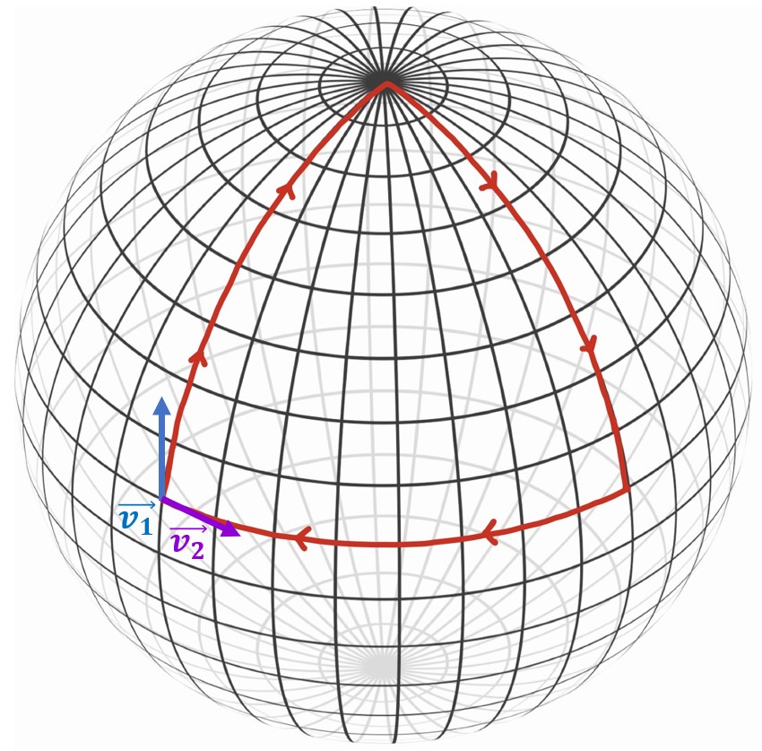
Figure 1: Representation of the effect of curvature. By parallel transporting the vector $\vec{v_{1}}$ along a closed path (in red), we obtain the vector $v_{2}$. The initial and the parallel transported vector do not coincide due to curvature.

Torsion

The second geometric property is torsion Cartan:1922 ; Cartan:1923 ; Cartan:1924 ; Cartan:1925 . It is defined by

$$T^{\alpha}_{~{}\beta\gamma}\equiv 2\Gamma^{\alpha}_{~{}[\beta\gamma]}=\Gamma^{\alpha}_{~{}\beta\gamma}-\Gamma^{\alpha}_{~{}\gamma\beta}\;,$$ (5)

i.e., it emerges when the Christoffel symbols $\Gamma^{\alpha}_{~{}\beta\gamma}$ are not symmetric in the two lower indices. If torsion is present, then the parallelogram formed by the parallel transport of two vectors may not close, as represented in fig. 2. Indeed if we consider two infinitesimal vectors $A^{\mu}(x^{\nu})$ and $B^{\mu}(x^{\nu})$ and we parallel transport them along each other, we obtain (see e.g., also Yepez:2011bw ):

$$\begin{split}A^{\mu}(x^{\nu}+B^{\nu})=A^{\mu}(x^{\nu})-\Gamma^{\mu}_{~{}\alpha\beta}A^{\beta}B^{\alpha}\;,\\ B^{\mu}(x^{\nu}+A^{\nu})=B^{\mu}(x^{\nu})-\Gamma^{\mu}_{~{}\alpha\beta}B^{\beta}A^{\alpha}\;,\end{split}$$ (6)

where we used eq. (2). Hence the difference between the two transported vectors is :

$$\begin{split}&A^{\mu}(x^{\nu})+B^{\mu}(x^{\nu}+A^{\nu})-\big{(}B^{\mu}(x^{\nu})+A^{\mu}(x^{\nu}+B^{\nu})\big{)}\\ &=\Gamma^{\mu}_{~{}\alpha\beta}A^{\alpha}B^{\beta}-\Gamma^{\mu}_{~{}\alpha\beta}B^{\alpha}A^{\beta}=2\Gamma^{\mu}_{~{}[\alpha\beta]}A^{\alpha}B^{\beta}=T^{\mu}_{~{}\alpha\beta}A^{\alpha}B^{\beta}\;,\end{split}$$ (7)

i.e., it is determined by the torsion tensor $T^{\mu}_{~{}\alpha\beta}$.

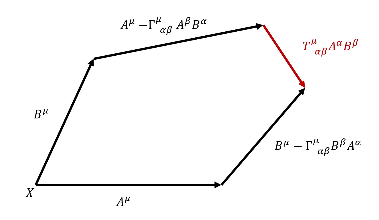
Figure 2: Representation of the effect of torsion. Two vectors $A^{\mu}$ and $B^{\mu}$ are parallel transported along each other. The non-closure of the resulting parallelogram, which is displayed in red, is proportional to torsion.

Non-metricity

Finally, the third geometric property is non-metricity. It emerges if the covariant derivative of the metric does not vanish and is defined by:

$$Q_{\gamma\alpha\beta}\equiv\nabla_{\gamma}g_{\alpha\beta}\;.$$ (8)

In the presence of non-metricity, the norm of the vector may change under parallel transport. Indeed, we can consider the length of a vector $\xi^{\alpha}$ that is parallel transported:

$$\begin{split}\frac{\mathrm{d}v^{2}}{\mathrm{d}s}&=\frac{\mathrm{d}(g_{\mu\nu}v^{\mu}v^{\nu})}{\mathrm{d}s}\\ &=\frac{\mathrm{d}x^{\alpha}}{\mathrm{d}s}\nabla_{\alpha}(g_{\mu\nu}v^{\mu}v^{\nu})\\ &=\frac{\mathrm{d}x^{\alpha}}{\mathrm{d}s}(\nabla_{\alpha}g_{\mu\nu}v^{\mu}v^{\nu}+2\underbrace{\nabla_{\alpha}v^{\mu}}_{=0}g_{\mu\nu}v^{\nu})\\ &=\frac{\mathrm{d}x^{\alpha}}{\mathrm{d}s}Q_{\alpha\mu\nu}v^{\mu}v^{\nu}\neq 0\;.\end{split}$$ (9)

To summarize, a schematic representation of curvature, torsion, and non-metricity is shown in fig. 3.

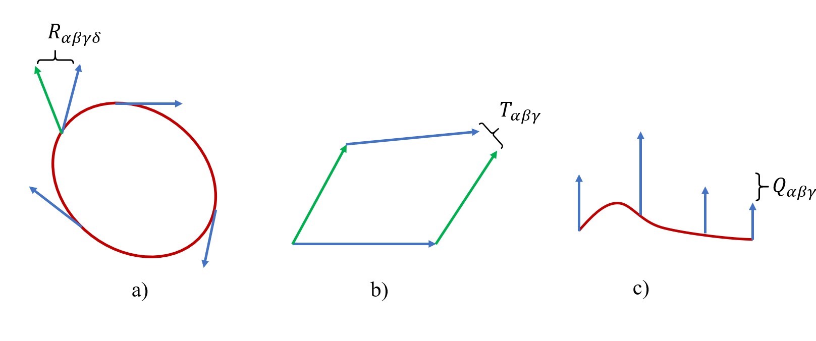
Figure 3: Schematic representation of the change of a vector under parallel transport due to the presence of: a) curvature b) torsion c) non-metricity. Figure inspired by BeltranJimenez:2019tjy .

Special case: Riemannian geometry

As a special case, it is possible to consider a connection $\mathring{\Gamma}^{\alpha}_{~{}\beta\gamma}$ with vanishing torsion and non-metricity:

$$Q_{\mu\alpha\beta}=\mathring{\nabla}_{\mu}g_{\alpha\beta}=0\;,\qquad T^{\alpha}_{\beta\gamma}=\mathring{\Gamma}^{\alpha}_{~{}\beta\gamma}-\mathring{\Gamma}^{\alpha}_{~{}\gamma\beta}=0\;,$$ (10)

where $\mathring{\nabla}$ is the covariant derivative associated with $\mathring{\Gamma}^{\alpha}_{~{}\beta\gamma}$. Once these conditions are imposed, the connection is uniquely determined as a function of the metric $g_{\mu\nu}$:

$$\mathring{\Gamma}^{\alpha}_{~{}\beta\gamma}=\frac{1}{2}g^{\alpha\mu}(\partial_{\beta}g_{\mu\gamma}+\partial_{\gamma}g_{\mu\beta}-\partial_{\mu}g_{\beta\gamma})\;.$$ (11)

The requirements (10) lead to a Riemannian geometry and $\mathring{\Gamma}^{\alpha}_{~{}\beta\gamma}$ is the Levi-Civita connection. According to eq. (4), the corresponding Riemann tensor reads:

$$\mathring{R}_{~{}\sigma\mu\nu}^{\rho}=\partial_{\mu}\mathring{\Gamma}_{~{}\nu\sigma}^{\rho}-\partial_{\nu}\mathring{\Gamma}_{~{}\mu\sigma}^{\rho}+\mathring{\Gamma}_{~{}\mu\lambda}^{\rho}\mathring{\Gamma}_{~{}\nu\sigma}^{\lambda}-\mathring{\Gamma}_{~{}\nu\lambda}^{\rho}\mathring{\Gamma}_{\mu\sigma}^{\lambda}\;.$$ (12)

Using the Levi-Civita connection $\mathring{\Gamma}^{\alpha}_{~{}\beta\gamma}$ leads to the metric formulation of GR. Since in this case second derivatives of the metric appear in eq. (12), one can call it a second-order formalism.

It is worth noting that there is an asymmetry between curvature on the one side and torsion/non-metricity on the other side. Whereas curvature does not influence torsion/non-metricity, eq. (3) shows that torsion and non-metricity contribute to curvature (see also computation in appendix B). Correspondingly, an assumption about the absence of torsion and/or non-metricity, displayed in eq. (10), has different consequences than assuming that curvature vanishes. We will elaborate on this point in section 2.3.

2.2 Decomposition of torsion and non-metricity

In full generality, we can decompose the connection into its Levi-Civita part and deviations from Riemannian geometry:

$$\Gamma^{\gamma}_{~{}\alpha\beta}=\mathring{\Gamma}^{\gamma}_{~{}\alpha\beta}(g)+J^{\gamma}_{~{}\alpha\beta}(Q)+K^{\gamma}_{~{}\alpha\beta}(T)\;.$$ (13)

Here $\mathring{\Gamma}^{\gamma}_{\alpha\beta}(g)$ is the Levi-Civita connection, which only depends on the metric, $K^{\gamma}_{~{}\alpha\beta}(T)$ corresponds to the contorsion tensor depending on the torsion, and $J^{\gamma}_{~{}\alpha\beta}(Q)$ is the disformation tensor depending on the non-metricity. Since contorsion $K^{\gamma}_{~{}\alpha\beta}$ is defined to be insensitive to non-metricity, it follows that $\nabla_{\alpha}g_{\mu\nu}|_{J^{\gamma}_{~{}\alpha\beta}=0}=0$. This condition determines contorsion as a function of torsion:

$$K_{\alpha\beta\gamma}=\frac{1}{2}(T_{\alpha\beta\gamma}+T_{\beta\alpha\gamma}+T_{\gamma\alpha\beta})\;,$$ (14)

where as usual $K_{\alpha\beta\gamma}\equiv g_{\alpha\sigma}K^{\sigma}_{~{}\beta\gamma}$. Similarly, we find the expression of disformation in terms of non-metricity by imposing that $\Gamma^{\gamma}_{~{}[\alpha\beta]}|_{J_{\alpha\beta\gamma}=0}=0$. This leads to:

$$J_{\alpha\mu\nu}=\frac{1}{2}(Q_{\alpha\mu\nu}-Q_{\nu\alpha\mu}-Q_{\mu\alpha\nu})\;.$$ (15)

Note that eq. (14) is sensitive to the convention (1) for the covariant derivative whereas eq. (15) is not. Contorsion is anti-symmetric in the first and last indices, $K_{\alpha\beta\gamma}=K_{[\alpha|\beta|\gamma]}$, while disformation is symmetric in last two indices, $J_{\alpha\beta\gamma}=J_{\alpha(\beta\gamma)}$.

We can invert relations (14) and (15) to express torsion in terms of contorsion and non-metricity in terms of disformation :

$$\begin{split}Q_{\alpha\beta\gamma}=-2J_{(\beta|\alpha|\gamma)}\;,\qquad T_{\alpha\beta\gamma}=2K_{\alpha[\beta\gamma]}\;.\end{split}$$ (16)

This shows that contorsion (respectively disformation) and torsion (respectively non-metricity) encode the same information, because we can go from one to the other with a bijective transformation. Therefore, we can either view $\Gamma^{\gamma}_{~{}\alpha\beta}$ as fundamental field or $T^{\gamma}_{~{}\alpha\beta}$ and $Q^{\gamma}_{~{}\alpha\beta}$. Practically, this means that varying the action with respect to $\Gamma^{\gamma}_{~{}\alpha\beta}$ is equivalent to a simultaneous variations with respect to $T^{\gamma}_{~{}\alpha\beta}$ and $Q^{\gamma}_{~{}\alpha\beta}$.

We can further split torsion and non-metricity in vector- and tensor-parts. For torsion, irreducible representations are given by Hehl:1994ue ; Obukhov:1997zd ; Shapiro:2001rz :

$$\text{the trace vector:\ }T^{\alpha}=g_{\mu\nu}T^{\mu\alpha\nu}\;,$$ (17)

$$\text{the pseudo trace axial vector:\ }\hat{T}^{\alpha}=\epsilon^{\alpha\beta\mu\nu}T_{\beta\mu\nu}\;,$$ (18)

$$\text{the pure tensor part:\ }t^{\alpha\beta\gamma}\text{\ that satisfies\ }g_{\mu\nu}t^{\mu\alpha\nu}=0=\epsilon^{\alpha\beta\mu\nu}t_{\beta\mu\nu}\;.$$ (19)

Torsion can be expressed uniquely in terms of these irreducible pieces as:

$$T_{\alpha\beta\gamma}=-\frac{2}{3}g_{\alpha[\beta}T_{\gamma]}+\frac{1}{6}\epsilon_{\alpha\beta\gamma\nu}\hat{T}^{\nu}+t_{\alpha\beta\gamma}\;.$$ (20)

Similarly, we can split non-metricity into three pieces Hehl:1994ue ; Obukhov:1997zd :

$$\text{a first vector:\ }Q^{\gamma}=g_{\alpha\beta}Q^{\gamma\alpha\beta}\;,$$ (21)

$$\text{a second vector:\ }\hat{Q}^{\gamma}=g_{\alpha\beta}Q^{\alpha\gamma\beta}\;,$$ (22)

$$\text{the pure tensor part: }q^{\alpha\beta\gamma}\text{\ that satisfies\ }g_{\alpha\beta}q^{\gamma\alpha\beta}=0=g_{\alpha\beta}q^{\alpha\gamma\beta}\;.$$ (23)

Note that this decomposition does not correspond to irreducible representations since a fully symmetric tensor can still be separated from the pure tensor part $q^{\alpha\beta\gamma}$ Hehl:1994ue ; Obukhov:1997zd . In what follows, however, it will not be useful to further split $q^{\alpha\beta\gamma}$. Non-metricity can be expressed uniquely in terms of the components of eqs. (21) to (23):

$$Q_{\alpha\beta\gamma}=\frac{1}{18}[g_{\beta\gamma}(5Q_{\alpha}-2\hat{Q}_{\alpha})+2g_{\alpha(\beta}(4\hat{Q}_{\gamma)}-Q_{\gamma)})]+q_{\alpha\beta\gamma}\;.$$ (24)

As is evident from (17) to (20), the mapping of the full torsion tensor $T_{\alpha\beta\gamma}$ to the irreducible components $T^{\alpha}$, $\hat{T}^{\alpha}$ and $t^{\alpha\beta\gamma}$ is bijective. Eqs. (21) to (24) show that an analogous statement holds for the full non-metricity tensor $Q_{\alpha\beta\gamma}$ and the contributions $Q^{\gamma}$, $\hat{Q}^{\gamma}$, and $q^{\alpha\beta\gamma}$. Since also the mapping between $T^{\gamma}_{~{}\alpha\beta}$ and $Q^{\gamma}_{~{}\alpha\beta}$ on the one hand and the full connection $\Gamma^{\gamma}_{~{}\alpha\beta}$ on the other hand is bijective, we conclude that a variation with respect to $\Gamma^{\gamma}_{~{}\alpha\beta}$ is equivalent to a simultaneous variations with respect to the $6$ tensors $T^{\alpha}$, $\hat{T}^{\alpha}$, $t^{\alpha\beta\gamma}$, $Q^{\gamma}$, $\hat{Q}^{\gamma}$ and $q^{\alpha\beta\gamma}$. Finally, let us discuss the number of independent components in each irreducible piece. First, $T_{\alpha\beta\gamma}$ is antisymmetric in its last two indices, yielding $4\times 6=24$ independent components. Because $T^{\alpha}$ and $\hat{T}^{\alpha}$ are vectors, they can only have $4$ independent terms, and $t^{\alpha\beta\gamma}$ then carries the remaining $16$ independent components. For non-metricity the number is higher because $Q_{\alpha\beta\gamma}$ is symmetric in the last two indices, leading to $4\times 10=40$ independent components. Following the same argument, $Q^{\alpha}$ and $\hat{Q}^{\alpha}$ each carry $4$ independent components while $q^{\alpha\beta\gamma}$ carries $32$. Overall, the sum reproduces $64$ independent components of the initial affine connection $\Gamma^{\alpha}_{~{}\beta\gamma}$, in accordance with bijectivity.

Using the decomposition (13) of the connection as well as formulas (86) - (90) from appendix A, we can split the Ricci scalar as follows (see also Langvik:2020nrs ):

$$\begin{split}R&=\mathring{R}+\mathring{\nabla}_{\alpha}(Q^{\alpha}-\hat{Q}^{\alpha}+2T^{\alpha})-\frac{2}{3}T_{\alpha}(T^{\alpha}+Q^{\alpha}-\hat{Q}^{\alpha})+\frac{1}{24}\hat{T}^{\alpha}\hat{T}_{\alpha}+\frac{1}{2}t^{\alpha\beta\gamma}t_{\alpha\beta\gamma}\\ &-\frac{11}{72}Q_{\alpha}Q^{\alpha}+\frac{1}{18}\hat{Q}_{\alpha}\hat{Q}^{\alpha}+\frac{2}{9}Q_{\alpha}\hat{Q}^{\alpha}+\frac{1}{4}q_{\alpha\beta\gamma}(q^{\alpha\beta\gamma}-2q^{\gamma\alpha\beta})+t_{\alpha\beta\gamma}q^{\beta\alpha\gamma},\end{split}$$ (25)

where $\mathring{R}=g_{\mu\nu}\mathring{R}^{\alpha}_{~{}\mu\alpha\nu}$ is the scalar curvature solely computed from the Levi-Civita connection $\mathring{\Gamma}^{\alpha}_{~{}~{}\beta\gamma}$, as derived from the Riemann tensor shown in eq. (12).

The scalar curvature $R$ obeys an interesting property: it is invariant under projective transformation, defined by Schroedinger:1950 ; Trautman1973 ; Sandberg:1975db ; Hehl:1976kv ; Trautmann1976 ; Hehl:1978 ; Hehl:1981 :

$$\Gamma^{\gamma}_{~{}\alpha\beta}\rightarrow\Gamma^{\gamma}_{~{}\alpha\beta}+\delta^{\gamma}_{\beta}A_{\alpha}\;,$$ (26)

with $A_{\alpha}=A_{\alpha}(x)$ an arbitrary covariant vector field. Geometrically, eq. (26) represents the most general transformation that changes the auto-parallel curves by a reparametrization of their affine parameter (see Iosifidis:2018zjj for details). Notably, most irreducible components are not invariant under eq. (26):

$$T^{\alpha}\rightarrow T^{\alpha}+3A^{\alpha},\quad\hat{T}^{\alpha}\rightarrow\hat{T}^{\alpha},\quad Q^{\alpha}\rightarrow Q^{\alpha}-8A^{\alpha},\quad\hat{Q}^{\alpha}\rightarrow\hat{Q}^{\alpha}-2A^{\alpha}\;,$$ (27)

but the combination that enters into the scalar curvature given in eq. (25), and correspondingly the Einstein-Hilbert action, are invariant. As long as an action remains unchanged under projective transformations, the connection $\Gamma^{\gamma}_{~{}\alpha\beta}$ cannot be uniquely determined by its equations of motion Schroedinger:1950 ; Trautman1973 ; Sandberg:1975db ; Hehl:1976kv ; Trautmann1976 ; Hehl:1978 ; Hehl:1981 . However, a general theory may not be invariant under the projective transformation, as will be discussed in section 3.

2.3 Classifying possible theories

We have seen that a generic geometry of spacetime can be characterized by the three properties: curvature, torsion and non-metricity. When devising a theory of gravity, one has to decide for each of these three concepts whether they should be included or excluded. Therefore, up to eight choices are available to us. Clearly, excluding all non-trivial geometry leads to a Minkowski spacetime and the absence of gravity, which leaves us with seven possibilities. As we shall discuss, all seven indeed lead to viable formulations of gravity, which are summarized in table 1.

Expanding on the introduction, we shall discuss them in the following. In doing so, we will briefly sketch how some of their properties can be derived. Our goal is to convey to the reader a rough idea of the underlying calculations in a manner that is as concise as possible. Therefore, we leave out many details and equations in the present subsection 2.3 are only symbolic. Precise computations for the metric-affine formulation will be presented in section 3. For teleparallel theories we refer the reader to the references displayed subsequently.

Formulation of gravity	$R_{\alpha\beta\gamma\delta}$	$T_{\alpha\beta\gamma}$	$Q_{\alpha\beta\gamma}$	Equivalent to metric GR for arbitrary coefficients of $T^{2}$, $QT$, $Q^{2}$
Metric-affine Hehl:1976kt ; Hehl:1976kv ; Hehl:1976my ; Hehl:1977fj				Yes
Einstein-Cartan Cartan:1922 ; Cartan:1923 ; Cartan:1924 ; Cartan:1925 ; Einstein:1928 ; Einstein:19282			$=0$	Yes
Weyl Weyl:1918 ; Weyl:1922 ; Eddington:1923		$=0$		Yes
Metric Einstein:1915		$=0$	$=0$	(Not applicable)
Generic teleparallel BeltranJimenez:2019odq	$=0$			No
Metric teleparallel Einstein:1928 ; Einstein:19282 ; Moller:1961 ; Pellegrini:1963 ; Hayashi:1967se ; Cho:1975dh ; Hayashi:1979qx	$=0$		$=0$	No
Symmetric teleparallel Nester:1998mp	$=0$	$=0$		No

Table 1: List of different formulations of gravity. Properties are summarized, with a display of the vanishing of tensorial quantities. As in the text, $T^{2}$ stands for an arbitrary invariant composed of torsion $T_{\alpha\beta\gamma}$, and analogous statements apply to $QT$ and $Q^{2}$.

.

2.3.1 Theories with curvature

First, we shall discuss the four possible formulations that feature curvature. Clearly, excluding a priori both torsion and non-metricity results in the most commonly-used metric version of GR Einstein:1915 . In the absence of matter, its action is given by

$$\mathcal{L}_{\text{metric}}\sim\mathring{R}\;,$$ (28)

where $\mathring{R}$ is the curvature determined by the Levi-Civita connection, as defined in eq. (12). Next, we shall discuss the effect of including the other two geometric concepts. As reviewed in the introduction, adding non-metricity in addition to curvature leads to Weyl gravity Weyl:1918 ; Weyl:1922 , whereas a theory that features both torsion and curvature corresponds to the Einstein-Cartan formulation Cartan:1922 ; Cartan:1923 ; Cartan:1924 ; Cartan:1925 ; Einstein:1928 ; Einstein:19282 . Including all three geometric properties – curvature, torsion and non-metricity – results in a general metric-affine theory of gravity Hehl:1976kt ; Hehl:1976kv ; Hehl:1976my ; Hehl:1977fj ; see Hehl:1980 ; Hehl:1994ue ; Blagojevic:2002 ; Blagojevic:2003cg ; Obukhov:2018bmf for reviews.

Once torsion and/or non-metricity are included, the next question is what action one should use. An obvious choice is

$$\mathcal{L}_{\text{affine, specific}}\sim R\;,$$ (29)

where the corresponding Riemann tensor is defined in (4). Such a model, in which the purely gravitational action only consists of the Ricci scalar, leads to the Palatini version of GR (see discussion in section 1). As derived in eq. (25), we can split $R$ in a part $\mathring{R}$ that solely depends on the Levi-Civita connection $\mathring{\Gamma}^{\alpha}_{~{}~{}\beta\gamma}$ and quadratic invariants composed of torsion and/or non-metricity. We note that we can leave out contributions of the form $\mathring{\nabla}T^{\alpha}$ and $\mathring{\nabla}Q^{\alpha}$ since they only lead to boundary terms. Moreover, the quadratic contributions of torsion and non-metricity in eq. (29) have fixed coefficients (e.g., $Q_{\alpha}Q^{\alpha}$ comes with a factor of $-11/72$; see eq. (25)). However, we can be more general and include quadratic invariants with arbitrary coefficients. We will give the precise form of the resulting action in section 3 (see eq. (40)). For now, we shall content ourselves with briefly sketching the effect of including torsion and/or non-metricity. To this end, it suffices to write symbolically

$$\mathcal{L}_{\text{affine}}\sim\mathring{R}+c_{TT}T^{2}+c_{QQ}Q^{2}+c_{TQ}TQ\;,$$ (30)

where $T$ and $Q$ stand for any tensor linear in torsion and non-metricity, respectively. (For example, $T$ can represent $T^{\alpha},\hat{T}^{\alpha}$ and $t^{\alpha\beta\gamma}$). Moreover, $c_{TT}$, $c_{QQ}$ and $c_{TQ}$ are arbitrary coefficients. Now we can determine torsion and/or non-metricity by their equations of motion. For the action (30), a solution is given by

$$T=0\;,\qquad Q=0\;.$$ (31)

Thus, the two additional geometric properties vanish dynamically in the absence of matter. This shows why in purely gravitational theories of the form (30), the metric-affine formulation as well as its two special cases Einstein-Cartan and Weyl-gravity are equivalent to the most commonly-used metric version of GR.

Next we shall repeat the previous discussion in the presence of matter, where we use a scalar field $h$ as an example. Motivated by an analogy to the Higgs field of the Standard Model in unitary gauge, we shall assume that $h$ possesses a $Z_{2}$-symmetry $h\rightarrow-h$. Apart from this property, however, $h$ will represent in the present work a generic scalar field which can be different from the Higgs field. In the metric formulation, the action for coupling $h$ to gravity is given by

$$\mathcal{L}_{\text{metric}}\sim\mathring{R}+\xi h^{2}\mathring{R}+\mathcal{L}_{\text{m}}\;,$$ (32)

which reduces to eq. (28) in the absence of matter. Here $\xi$ parametrizes a non-minimal coupling of the scalar field to gravity and $\mathcal{L}_{\text{m}}$ can contain all operators in the matter sector that are independent of the Christoffel symbols. Once torsion and/or non-metricity are included, the generalization of eq. (29) leads to

$$\mathcal{L}_{\text{affine, specific}}\sim R+\xi h^{2}R+\mathcal{L}_{\text{m}}\;.$$ (33)

Again we can use eq. (25) to split $R$ in a Levi-Civita part $\mathring{R}$ and terms involving torsion and/or non-metricity. Due to the non-minimal coupling of $h$ to $R$, now also the terms of the form $\mathring{\nabla}_{\alpha}T^{\alpha}$ and $\mathring{\nabla}_{\alpha}Q^{\alpha}$ give a non-trivial contribution. As before, we replace specific by arbitrary coefficients, and so the generalization of eq. (30) in the presence of matter yields

$$\begin{split}\mathcal{L}_{\text{affine}}\sim&\mathring{R}+\xi h^{2}\mathring{R}+(c_{TT}+\tilde{c}_{TT}h^{2})T^{2}+(c_{QQ}+\tilde{c}_{QQ}h^{2})Q^{2}+(c_{TQ}+\tilde{c}_{TQ}h^{2})TQ\\ &+\xi_{T}h^{2}\mathring{\nabla}T+\xi_{Q}h^{2}\mathring{\nabla}Q+\mathcal{L}_{\text{m}}\;.\end{split}$$ (34)

It is important to note that the number of coefficients describing a non-minimal coupling of matter to gravity has significantly increased. Whereas only one such parameter exists in metric gravity ($\xi$), many more analogous contributions emerge in the metric-affine formulation. Once torsion and/or non-metricity are present, there is no reason to exclude the couplings of matter to gravity, which are all on the same footing as the single non-minimal coupling term in metric gravity.

In eq. (34), the equations of motion for $J$ and $Q$ yield a non-trivial result:

$$T\sim\partial h^{2}\;,\qquad Q\sim\partial h^{2}\;.$$ (35)

The significance of this finding is twofold. First, it shows how torsion and/or non-metricity are sourced once appropriate couplings to matter, such as a scalar field, are added. Secondly, the solution (35) is algebraic. Thus, torsion and non-metricity do not propagate, and also metric-affine gravity only features excitations of a massless graviton. As a particular consequence, we can plug the solution (35) back into the action (34):

$$\mathcal{L}_{\text{affine}}\sim\mathring{R}+\xi h^{2}\mathring{R}+f(h)\left(\partial h^{2}\right)^{2}+\mathcal{L}_{\text{m}}\;,$$ (36)

where $f(h)$ is a function of $h$ that is determined by the parameters appearing in the action (34). We can call eq. (36) the equivalent metric theory, in which the effects of torsion and/or non-metricity are replaced by specific additional operators in the matter sector.

In summary, we have outlined why in the presence of matter, the different formulations of gravity that feature curvature are no longer equivalent. Their difference can be reduced to specific additional interactions in the matter sector, which feature a number of a priori unknown coupling constants. Finally, we note that the limits of excluding torsion and/or non-metricity are smooth, i.e., the following two procedures lead to the same result. On the one hand, one can assume a priori that torsion and/or non-metricity vanish. On the other hand, it is equivalent to put in the Lagrangian the coefficients of all terms involving $T$ and/or $Q$ to zero. To obtain the Einstein-Cartan formulation for example, one can simply set in eq. (34) all coefficients involving $Q$ to zero and arrive at an accordingly simplified equivalent metric theory (36). A summary of the relation between the different theories of gravity with curvature is given in fig. 4.

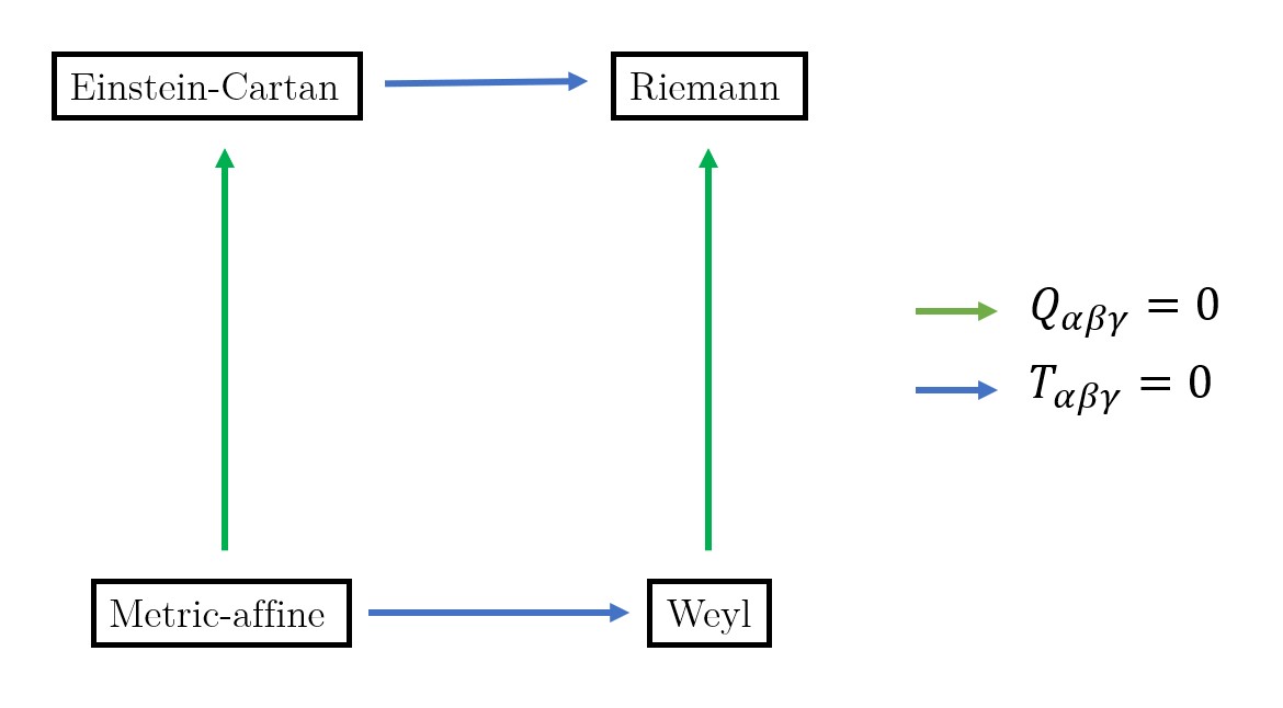
Figure 4: Diagram of relations between different formulations of gravity with curvature. Starting from the most general class of metric-affine theories of gravity in the lower, left corner; one can obtain specific limits by imposing that torsion or non-metricity vanish.

2.3.2 Teleparallel theories

Next we shall turn to three possible teleparallel formulations of GR, in which curvature is excluded; see Maluf:2013gaa ; Aldrovandi:2013wha ; Heisenberg:2018vsk ; Krssak:2018ywd ; Bahamonde:2021gfp for reviews. First, a metric teleparallel theory was proposed, in which only torsion is present and non-metricity is assumed to vanish Einstein:1928 ; Einstein:19282 ; Moller:1961 ; Pellegrini:1963 ; Hayashi:1967se ; Cho:1975dh ; Hayashi:1979qx . Subsequently, a symmetric teleparallel formulation was developed that exclusively features non-metricity Nester:1998mp . Only very recently, a general teleparallel theory was constructed that simultaneously contains both torsion and non-metricity BeltranJimenez:2019odq . The assumption of vanishing curvature has different implications than setting to zero torsion and/or non-metricity. Assuming that the latter two quantities vanish in a metric-affine formulation does not have any effects on the Levi-Civita curvature $\mathring{R}$. In contrast, this is not the case for the assumption of teleparallelism, as one can anticipate from eq. (25), which shows that curvature is the sum of a Levi-Civita part $\mathring{R}$ and contributions of torsion and non-metricity. Therefore, setting to zero curvature can constrain $\mathring{R}$ in terms of torsion and/or non-metricity. In the following, we shall briefly sketch how this comes about, and we refer the reader e.g., to BeltranJimenez:2017tkd ; BeltranJimenez:2018vdo ; Heisenberg:2018vsk ; BeltranJimenez:2019odq ; Bahamonde:2021gfp for more details.

As in BeltranJimenez:2019odq , we will include both torsion and non-metricity. First we consider the theory in the absence of matter, where we follow Bahamonde:2021gfp . In analogy to eq. (29), we start from the action

$$\mathcal{L}_{\text{teleparallel, specific}}\sim-T^{2}-Q^{2}-TQ+\lambda\left(\mathring{R}+T^{2}+Q^{2}+TQ+\mathring{\nabla}T+\mathring{\nabla}Q\right)\;,$$ (37)

where the Lagrange multiplier $\lambda=\lambda(x)$ enforces the constraint of vanishing curvature. Moreover, the coefficients of the quadratic invariants in torsion and/or non-metricity are fixed according to eq. (25), up to a sign change in the first three terms. The motivation for this specific choice of parameters comes from ensuring equivalence to metric GR. Namely, we can plug the constraint $-T^{2}-Q^{2}-TQ=\mathring{R}+\mathring{\nabla}T+\mathring{\nabla}Q$ back in the action (37) to obtain

$$\mathcal{L}_{\text{teleparallel, specific}}\sim\mathring{R}+\mathring{\nabla}T+\mathring{\nabla}Q\;.$$ (38)

Up to a boundary term, this coincides with the result (28) of metric gravity. Therefore, eq. (37) is the action of the General Teleparallel Equivalent of GR (GTEGR) BeltranJimenez:2019odq . Leaving out all terms involving non-metricity leads to the Metric Teleparallel Equivalent of GR Einstein:1928 ; Einstein:19282 ; Moller:1961 ; Pellegrini:1963 ; Hayashi:1967se ; Cho:1975dh ; Hayashi:1979qx . Correspondingly, omitting all contributions of torsion yields the Symmetric Teleparallel Equivalent of GR Nester:1998mp . We shall not explicitly discuss how matter can be coupled to the different teleparallel equivalents of GR but only refer the reader to the literature. It was noted early on that in torsionful theories an issue can arise due to fermions Hayashi:1979qx but that a consistent interaction with matter can be achieved with an appropriate choice of coupling prescription; see Hayashi:1979qx ; deAndrade:1997cj ; deAndrade:1997gka ; deAndrade:2000kr ; deAndrade:2001vx ; Obukhov:2002tm ; Maluf:2003fs ; Mielke:2004gg ; Mosna:2003rx ; Obukhov:2004hv ; Aldrovandi:2013wha for studies excluding non-metricity and Adak:2008gd ; BeltranJimenez:2017tkd ; BeltranJimenez:2018vdo ; Jimenez:2019woj ; Delhom:2020hkb ; BeltranJimenez:2020sih for investigations without this restriction. We note that the Symmetric Teleparallel Equivalent of GR may evade some of the ambiguities caused by torsion BeltranJimenez:2017tkd ; BeltranJimenez:2018vdo ; Jimenez:2019woj ; BeltranJimenez:2020sih .

Finally, we shall give a brief outlook to generalizations of the Lagrangian (37). First, one can attempt to choose arbitrary coefficients in eq. (37), in analogy to our approach in the metric-affine case. For the case of vanishing non-metricity, this was already suggested in Hayashi:1979qx under the name New GR and symbolically reads

$$\mathcal{L}_{\text{teleparallel, generic}}\sim c_{TT}T^{2}+\lambda\left(\mathring{R}+T^{2}+\mathring{\nabla}T\right)\;,$$ (39)

where we note that the parameters in the constraint remain fixed. However, issues were discovered in this model Kopczynski:1982 ; Kuhfuss:1986rb ; Nester:1988 ; Cheng:1988zg . Moreover, it generically contains additional propagating degrees of freedom Kuhfuss:1986rb , and so it differs from metric GR already in the absence of matter and does not correspond to an equivalent formulation. Analogous statements, namely that additional propagating degrees of freedom emerge for generic parameter choices, hold in the other teleparallel models. For a theory that only features non-metricity this question was studied in BeltranJimenez:2017tkd ; BeltranJimenez:2018vdo , where the term Newer GR was introduced, and a model with both torsion and non-metricity was investigated in BeltranJimenez:2019odq . Thus, even though the geometry of a generic teleparallel theory is simpler than in the metric-affine case, its particle spectrum is more involved. Starting from a generic gravitational Lagrangian (39), equivalence with metric GR is only achieved for specific values of the coefficients. These parameter choices can arise as a result of symmetries BeltranJimenez:2017tkd ; BeltranJimenez:2018vdo ; Jimenez:2019woj ; BeltranJimenez:2019odq . Applications of teleparallel gravity to cosmology, e.g., with respect to inflation and dark energy, can for example be found in Bengochea:2008gz ; Linder:2010py ; Myrzakulov:2010vz ; Wu:2010xk ; Chen:2010va ; Bengochea:2010sg ; Dent:2010nbw ; Li:2011wu ; Cai:2011tc ; Sharif:2011bi ; Hohmann:2017jao ; BeltranJimenez:2017tkd ; Jarv:2018bgs ; BeltranJimenez:2018vdo ; Dialektopoulos:2019mtr ; BeltranJimenez:2019tme ; Raatikainen:2019qey ; DAmbrosio:2020nev ; Bose:2020xdz ; DAmbrosio:2021pnd ; Solanki:2022rwu ; Capozziello:2022vyd ; see also Cai:2015emx for a review.

A summary of the relation between the different theories of gravity without curvature is given in fig. 5.

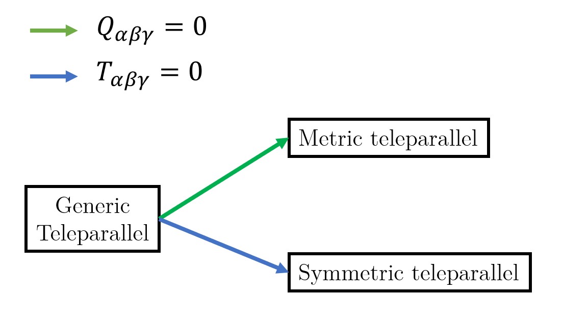
Figure 5: Diagram of relations between different formulations of gravity without curvature. Starting from the most general class of teleparallel theories of gravity on the left, one can obtain specific limits by imposing that torsion or non-metricity vanish.

2.4 Selection rules

In the preceding section, we have already outlined schematically the class of models that we shall investigate. In order to proceed systematically, we will now review the criteria developed in Karananas:2021zkl for constructing an action of matter coupled to gravity. Only torsion was considered in Karananas:2021zkl but the conditions equally well apply to a metric-affine formulation in which both torsion and non-metricity are present. In addition to (implicit) requirements of Lorentz invariance and locality, the criteria of Karananas:2021zkl demand the following:

1. The purely gravitational part of the action should only feature operators of mass dimension not greater than $2$.

2. The matter Lagrangian should be renormalizable in the flat space limit, i.e., for $g_{\mu\nu}=\eta_{\mu\nu}$ and $\Gamma_{~{}~{}\mu\lambda}^{\alpha}=0$.

3. The interaction of gravity and matter should only happen via operators of mass dimension not greater than $4$.

Subsequently, we shall discuss their motivation and implications.

Since torsion and non-metricity have mass dimension $1$ and curvature has mass dimension $2$, criterion 1.) implies that terms at most quadratic in torsion/non-metricity and linear in curvature can be included. Following the arguments of the preceding section, one can equivalently say that this condition arises from the decomposition (25) of curvature. Namely, it amounts to including contributions analogous to those already contained in curvature but with arbitrary coefficients. The purpose of criterion 1.) is to ensure equivalence with metric GR in the absence of matter. Correspondingly, it excludes terms that are quadratic or higher in curvature since they generically lead to new propagating degrees of freedom. What is more, some of these additional particles also cause inconsistencies, in particular since they correspond to ghosts, i.e., have a kinetic term with a wrong sign. Note that this is already the case in metric gravity Stelle:1977ry , and numerous additional problematic terms arise in the presence of torsion Neville:1978bk ; Neville:1979rb ; Sezgin:1979zf ; Hayashi:1979wj ; Hayashi:1980qp . We must mention, however, that certain combinations of curvature-squared contribution only lead to new propagating degrees of freedom that are healthy; see Sezgin:1981xs ; Kuhfuss:1986rb ; Yo:1999ex ; Yo:2001sy ; Nair:2008yh ; Nikiforova:2009qr ; Karananas:2014pxa ; Karananas:2016ltn ; Obukhov:2017pxa ; Blagojevic:2017ssv ; Blagojevic:2018dpz ; Lin:2018awc ; Jimenez:2019qjc ; Lin:2019ugq for studies in the presence of torsion and BeltranJimenez:2019acz ; Aoki:2019rvi ; Percacci:2019hxn ; BeltranJimenez:2020sqf ; Marzo:2021esg ; Marzo:2021iok ; Baldazzi:2021kaf for extensions to non-metricity. Moreover, it is possible to construct theories with terms that are quadratic in curvature that do not feature at all any additional propagating degrees of freedom Karananas:2021zkl . Therefore, criterion 1.) is sufficient but not strictly necessary for ensuring that the gravitational theory is equivalent to metric GR in pure gravity.

Criterion 2.) implies that the matter sector only contains operators of mass dimension not greater than $4$. This assumption is crucial for the predictiveness of our setup. Without it, one could have added from the beginning generic higher-dimensional operators to our model and the specific higher-dimensional operators that arise due to torsion and non-metricity would be meaningless. Needless to say, the validity of this approach, in which the matter Lagrangian solely features those non-renormalizable operators that result from torsion and non-metricity, remains to be checked. At least in principle, this can be done by systematically exploring the predictions that result from the specific higher-dimensional interactions and then comparing them with observations and experiments. In the present paper, we lay the groundwork for such studies by explicitly deriving the set of predicted operators in the scalar sector.

Criterion 3.) can be regarded as an attempt to define the notion of non-minimal coupling independently of the formulation of GR. In metric gravity, there is a unique operator for coupling a $Z_{2}$-symmetric scalar field $h$ non-minimally to GR, namely $h^{2}\mathring{R}$ (see eq. (32)). Since it has mass dimension 4, criterion 3.) aims at generalizing the notion of non-minimal coupling by selecting all terms that are on the same footing as the non-minimal coupling in metric GR. However, criterion 3.) is not crucial for our approach. It can be relaxed, as long as one makes sure that the coupling of matter and gravity does not lead to any additional propagating degrees of freedom. Correspondingly, we shall keep our discussion general and not impose criterion 3.) in some parts of the present work. It will only be implemented from section 3.3 on.

3 Scalar field coupled to metric-affine gravity

3.1 The theory

Next, we shall consider a scalar field $h$ coupled to gravity and write down the most general action obeying selection rules 1.) and 2.). We will rely on a decomposition of torsion and non-metricity into vector- and tensor-parts, as shown in eqs. (17) to (24). This method, which was introduced in Obukhov:1997zd , makes it significantly easier to solve the equations of motion. We get the action

$$S= \int\mathrm{d}^{4}x\sqrt{-g}\Big{[}\frac{1}{2}\Omega^{2}(h)\mathring{R}-\frac{1}{2}\tilde{K}(h)g^{\alpha\beta}\partial_{\alpha}h\partial_{\beta}h-V(h)$$ (40a)

$$+A_{1}(h)\mathring{\nabla}_{\alpha}\hat{T}^{\alpha}+A_{2}(h)\mathring{\nabla}_{\alpha}T^{\alpha}+A_{3}(h)\mathring{\nabla}_{\alpha}\hat{Q}^{\alpha}+A_{4}(h)\mathring{\nabla}_{\alpha}Q^{\alpha}$$ (40b)

$$+B_{1}(h)Q_{\alpha}Q^{\alpha}+B_{2}(h)\hat{Q}_{\alpha}\hat{Q}^{\alpha}+B_{3}(h)Q_{\alpha}\hat{Q}^{\alpha}+B_{4}(h)q_{\alpha\beta\gamma}q^{\alpha\beta\gamma}+B_{5}(h)q_{\alpha\beta\gamma}q^{\beta\alpha\gamma}$$ (40c)

$$+C_{1}(h)T_{\alpha}T^{\alpha}+C_{2}(h)\hat{T}_{\alpha}\hat{T}^{\alpha}+C_{3}(h)T_{\alpha}\hat{T}^{\alpha}+C_{4}(h)t_{\alpha\beta\gamma}t^{\alpha\beta\gamma}$$ (40d)

$$+D_{1}(h)\epsilon_{\alpha\beta\gamma\delta}t^{\alpha\beta\lambda}t^{\gamma\delta}_{~{}~{}\lambda}+D_{2}(h)\epsilon_{\alpha\beta\gamma\delta}q^{\alpha\beta\lambda}q^{\gamma\delta}_{~{}~{}\lambda}+D_{3}(h)\epsilon_{\alpha\beta\gamma\delta}q^{\alpha\beta\lambda}t^{\gamma\delta}_{~{}~{}\lambda}$$ (40e)

$$+E_{1}(h)T_{\alpha}Q^{\alpha}+E_{2}(h)\hat{T}_{\alpha}Q^{\alpha}+E_{3}(h)T_{\alpha}\hat{Q}^{\alpha}+E_{4}(h)\hat{T}_{\alpha}\hat{Q}^{\alpha}+E_{5}(h)t^{\alpha\beta\gamma}q_{\beta\alpha\gamma}\Big{]}.$$ (40f)

Since at this point we have not yet enforced selection rule 3.) of section 2.4, $\Omega^{2}(h)$, $\tilde{K}(h)$, $A_{i}(h)$, $B_{i}(h)$, $C_{i}(h)$, $D_{i}(h)$ and $E_{i}(h)$ in eq. (40) represent arbitrary functions of $h$. Besides, some of the possible non-vanishing terms have not been included in the action, such as e.g., $t_{\alpha\beta\gamma}t^{\beta\alpha\gamma}$. The reason is that they are linearly dependent on terms that are already present. For more details, we refer the reader to appendix C, where the independence of terms is discussed. Notice that for generic choices of coefficient functions, the action eq. (40) is not invariant under the projective transformation shown in eq. (26). Thus, the connection can be uniquely determined by its equations of motion.

Let us briefly comment on related works in metric-affine gravity. A general action that features all independent invariants composed of torsion and non-metricity was already introduced in Pagani:2015ema , where torsion and non-metricity were not split into pure vector- and tensor-parts. The matter sector was not made explicit in Pagani:2015ema , and so the functions $\Omega^{2}(h)$, $\tilde{K}(h)$ and $A_{i}(h)$ were not present. The action proposed in Pagani:2015ema was further studied in Iosifidis:2021bad and solutions for torsion and non-metricity were derived in terms of energy-momentum- and hypermomentum-tensors. Unlike in the present work, the paper Iosifidis:2021bad employed a method for finding solutions that does not require the separation of pure tensor parts Iosifidis:2021ili ; Iosifidis:2021kwd .

3.2 Derivation of equivalent metric theory

We can now vary the action given in eq. (40) with respect to the six tensors $T^{\alpha}$, $\hat{T}^{\alpha}$, $t^{\alpha\beta\gamma}$, $Q^{\gamma}$, $\hat{Q}^{\gamma}$ and $q^{\alpha\beta\gamma}$, as discussed in section 2.2. We obtain the following equations of motion:

$$\begin{split}&2C_{2}(h)\hat{T}^{\alpha}+C_{3}(h)T^{\alpha}+E_{2}(h)Q^{\alpha}+E_{4}(h)\hat{Q}^{\alpha}=A_{1}^{\prime}(h)\partial^{\alpha}h\;,\\ &2C_{1}(h)T^{\alpha}+C_{3}(h)\hat{T}^{\alpha}+E_{1}(h)Q^{\alpha}+E_{3}(h)\hat{Q}^{\alpha}=A_{2}^{\prime}(h)\partial^{\alpha}h\;,\\ &2B_{2}(h)\hat{Q}^{\alpha}+B_{3}(h)Q^{\alpha}+E_{3}(h)T^{\alpha}+E_{4}(h)\hat{T}^{\alpha}=A_{3}^{\prime}(h)\partial^{\alpha}h\;,\\ &2B_{1}(h)Q^{\alpha}+B_{3}(h)\hat{Q}^{\alpha}+E_{1}(h)T^{\alpha}+E_{2}(h)\hat{T}^{\alpha}=A_{4}^{\prime}(h)\partial^{\alpha}h\;,\\ &2B_{4}(h)q_{\alpha\beta\gamma}+2B_{5}(h)q_{(\beta\alpha)\gamma}+2D_{2}(h)\epsilon_{\alpha\lambda\delta(\beta}q^{\lambda\delta}_{~{}~{}\gamma)}+D_{3}(h)\epsilon_{\alpha\lambda\delta(\beta}t^{\lambda\delta}_{~{}~{}\gamma)}-E_{5}(h)t_{(\beta\gamma)\alpha}=0\;,\\ &2C_{4}(h)t_{\alpha\beta\gamma}+2D_{1}(h)\epsilon_{\alpha\lambda\delta[\beta}t^{\lambda\delta}_{~{}~{}\gamma]}+D_{3}(h)\epsilon_{\alpha\lambda\delta[\beta}q^{\lambda\delta}_{~{}~{}\gamma]}+E_{5}(h)q_{[\beta\gamma]\alpha}=0\;,\end{split}$$ (41)

where prime denotes derivative with respect to $h$. Solutions can be found explicitly as the equations of motion are algebraic. We first notice that there are no source terms for the pure tensor parts, hence they simply vanish. On the contrary, the vector parts $T^{\alpha}$, $\hat{T}^{\alpha}$, $Q^{\alpha}$ and $\hat{Q}^{\alpha}$ do not vanish because of the presence of source terms $A_{i}(h)$. We obtain the solutions::

$$Q^{\alpha}=\frac{V}{Z}\partial^{\alpha}h\;,\qquad\hat{Q}^{\alpha}=\frac{W}{Z}\partial^{\alpha}h\;,\qquad T^{\alpha}=\frac{X}{Z}\partial^{\alpha}h\;,\qquad\hat{T}^{\alpha}=\frac{Y}{Z}\partial^{\alpha}h\;,\qquad t_{\alpha\beta\gamma}=q_{\alpha\beta\gamma}=0\;.$$ (42)

The common denominator reads

$$\begin{split}Z&=B_{3}^{2}(4C_{1}C_{2}-C_{3}^{2})+4B_{2}C_{2}E_{1}^{2}-4B_{2}C_{3}E_{1}E_{2}+4B_{2}C_{1}E_{2}^{2}-E_{2}^{2}E_{3}^{2}+2E_{1}E_{2}E_{3}E_{4}\\ &-E_{1}^{2}E_{4}^{2}+B_{3}(-4C_{2}E_{1}E_{3}+2C_{3}E_{2}E_{3}+2C_{3}E_{1}E_{4}-4C_{1}E_{2}E_{4})+4B_{1}(B_{2}(-4C_{1}C_{2}+C_{3}^{2})\\ &+C_{2}E_{3}^{2}-C_{3}E_{3}E_{4}+C_{1}E_{4}^{2})\;,\end{split}$$ (43)

and the numerators are:

$$\begin{split}V&=4A^{\prime}_{2}B_{2}C_{2}E_{1}-2A^{\prime}_{1}B_{2}C_{3}E_{1}+4A^{\prime}_{1}B_{2}C_{1}E_{2}-2A^{\prime}_{2}B_{2}C_{3}E_{2}-2A^{\prime}_{2}B_{3}C_{2}E_{3}+A^{\prime}_{1}B_{3}C_{3}E_{3}\\ &-A^{\prime}_{1}E_{2}E_{3}^{2}-2A^{\prime}_{1}B_{3}C_{1}E_{4}+A^{\prime}_{2}B_{3}C_{3}E_{4}+A^{\prime}_{1}E_{1}E_{3}E_{4}+A^{\prime}_{2}E_{2}E_{3}E_{4}-A^{\prime}_{2}E_{1}E_{4}^{2}\\ &+A^{\prime}_{3}(4B_{3}C_{1}C_{2}-B_{3}C_{3}^{2}-2C_{2}E_{1}E_{3}+C_{3}E_{2}E_{3}+C_{3}E_{1}E_{4}-2C_{1}E_{2}E_{4})\\ &+2A^{\prime}_{4}(B_{2}(-4C_{1}C_{2}+C_{3}^{2})+C_{2}E_{3}^{2}-C_{3}E_{3}E_{4}+C_{1}E_{4}^{2})\;,\end{split}$$ (44)

$$\begin{split}W&=-2A^{\prime}_{2}B_{3}C_{2}E_{1}+A^{\prime}_{1}B_{3}C_{3}E_{1}-2A^{\prime}_{1}B_{3}C_{1}E_{2}+A^{\prime}_{2}B_{3}C_{3}E_{2}+2A^{\prime}_{3}(B_{1}(-4C_{1}C_{2}+C_{3}^{2})+C_{2}E_{1}^{2}\\ &-C_{3}E_{1}E_{2}+C_{1}E_{2}^{2})+4A^{\prime}_{2}B_{1}C_{2}E_{3}-2A^{\prime}_{1}B_{1}C_{3}E_{3}+A^{\prime}_{1}E_{1}E_{2}E_{3}-A^{\prime}_{2}E_{2}^{2}E_{3}+4A^{\prime}_{1}B_{1}C_{1}E_{4}\\ &-2A^{\prime}_{2}B_{1}C_{3}E_{4}-A^{\prime}_{1}E_{1}^{2}E_{4}+A^{\prime}_{2}E_{1}E_{2}E_{4}+A^{\prime}_{4}(4B_{3}C_{1}C_{2}-B_{3}C_{3}^{2}-2C_{2}E_{1}E_{3}+C_{3}E_{2}E_{3}\\ &+C_{3}E_{1}E_{4}-2C_{1}E_{2}E_{4})\;,\end{split}$$ (45)

$$\begin{split}X&=4A^{\prime}_{4}B_{2}C_{2}E_{1}-2A^{\prime}_{3}B_{3}C_{2}E_{1}-2A^{\prime}_{4}B_{2}C_{3}E_{2}+A^{\prime}_{3}B_{3}C_{3}E_{2}+4A^{\prime}_{3}B_{1}C_{2}E_{3}-2A^{\prime}_{4}B_{3}C_{2}E_{3}\\ &-A^{\prime}_{3}E_{2}^{2}E_{3}-2A^{\prime}_{3}B_{1}C_{3}E_{4}+A^{\prime}_{4}B_{3}C_{3}E_{4}+A^{\prime}_{3}E_{1}E_{2}E_{4}+A^{\prime}_{4}E_{2}E_{3}E_{4}-A^{\prime}_{4}E_{1}E_{4}^{2}\\ &+A^{\prime}_{1}(4B_{1}B_{2}C_{3}-B_{3}^{2}C_{3}-2B_{2}E_{1}E_{2}+B_{3}E_{2}E_{3}+B_{3}E_{1}E_{4}-2B_{1}E_{3}E_{4})\\ &+2A^{\prime}_{2}(B_{3}^{2}C_{2}+B_{2}E_{2}^{2}-B_{3}E_{2}E_{4}+B_{1}(-4B_{2}C_{2}+E_{4}^{2}))\;,\end{split}$$ (46)

$$\begin{split}Y&=-2A^{\prime}_{4}B_{2}C_{3}E_{1}+A^{\prime}_{3}B_{3}C_{3}E_{1}+4A^{\prime}_{4}B_{2}C_{1}E_{2}-2A^{\prime}_{3}B_{3}C_{1}E_{2}-2A^{\prime}_{3}B_{1}C_{3}E_{3}+A^{\prime}_{4}B_{3}C_{3}E_{3}\\ &+A^{\prime}_{3}E_{1}E_{2}E_{3}-A^{\prime}_{4}E_{2}E_{3}^{2}+2A^{\prime}_{1}(B_{3}^{2}C_{1}+B_{2}E_{1}^{2}-B_{3}E_{1}E_{3}+B_{1}(-4B_{2}C_{1}+E_{3}^{2}))+4A^{\prime}_{3}B_{1}C_{1}E_{4}\\ &-2A^{\prime}_{4}B_{3}C_{1}E_{4}-A^{\prime}_{3}E_{1}^{2}E_{4}+A^{\prime}_{4}E_{1}E_{3}E_{4}+A^{\prime}_{2}(4B_{1}B_{2}C_{3}-B_{3}^{2}C_{3}-2B_{2}E_{1}E_{2}+B_{3}E_{2}E_{3}\\ &+B_{3}E_{1}E_{4}-2B_{1}E_{3}E_{4})\;.\end{split}$$ (47)

The expressions for the numerators and denominator are quite long but the overall form of the solution for torsion and non-metricity is simple: they are proportional to $\partial^{\alpha}h$, as shown in eq. (42).

The fact that the pure tensor parts $t^{\alpha\beta\gamma}$ and $q^{\alpha\beta\gamma}$ vanish dynamically has a remarkable consequence. As is evident from eq. (40), the similarity between terms containing torsion and terms containing non-metricity is only broken because of the pure tensor parts and their different symmetry properties. Once $t^{\alpha\beta\gamma}$ and $q^{\alpha\beta\gamma}$ are absent, however, an exact correspondence emerges between a theory that only features torsion and a model that solely contains non-metricity. Thus, our criteria for the construction of an action of gravity coupled to matter lead to a full equivalence of the Einstein-Cartan and Weyl formulations. We will make this point explicit in section 3.4.

Summarizing what we did so far, we started from the most general action (40) according to the criteria presented in section 2.4. Torsion and non-metricity are included, therefore we can write new terms that are absent in the metric formulation of GR. We then solved for both torsion and non-metricity and found that they are proportional to the derivative of the scalar field. As next step, we can plug these solutions back into the action eq. (40). Then the new terms will give contributions to the kinetic term of the scalar field, i.e., we can map the effect of torsion and non-metricity to a modification of the kinetic term. We get

$$S= \int\mathrm{d}^{4}x\sqrt{-g}\left[\frac{1}{2}\Omega^{2}(h)\mathring{R}-\frac{1}{2}\hat{K}(h)g^{\alpha\beta}\partial_{\alpha}h\partial_{\beta}h-V(h)\right]\;,$$ (48)

where the modified kinetic term reads:

$$\begin{split}\hat{K}=\tilde{K}-2\frac{1}{Z^{2}}[&B_{1}V^{2}+B_{2}W^{2}+B_{3}VW+C_{1}X^{2}+C_{2}Y^{2}+C_{3}XY+E_{1}VX+E_{2}VY\\ &+E_{3}WX+E_{4}WY-Z(A^{\prime}_{1}Y+A^{\prime}_{2}X+A^{\prime}_{3}W+A^{\prime}_{4}V)]\;.\end{split}$$ (49)

Since our result only features the torsion- and non-metricity-free curvature $\mathring{R}$, which is fully determined in terms of the metric $g_{\mu\nu}$, we can call eq. (48) the equivalent metric theory: We are back to a situation where the metric $g_{\mu\nu}$ is the only degree of freedom in the gravity sector.

At this point we are still in the Jordan frame where the Ricci scalar $\mathring{R}$ is multiplied by $\Omega^{2}(h)$, meaning that the scalar field is non-minimally coupled to gravity. One may perform a conformal transformation in order to go to the Einstein frame, where the coupling to gravity is minimal Carroll:2004 :

$$\begin{split}&g_{\alpha\beta}\rightarrow\Omega^{-2}g_{\alpha\beta}\;,\\ &g^{\alpha\beta}\rightarrow\Omega^{2}g^{\alpha\beta}\;,\\ &\sqrt{-g}\rightarrow\Omega^{-4}\sqrt{-g}\;,\\ &g^{\alpha\beta}\mathring{R}_{\alpha\beta}\rightarrow\Omega^{2}[g^{\alpha\beta}\mathring{R}_{\alpha\beta}+6g^{\alpha\beta}(\mathring{\nabla}_{\alpha}\mathring{\nabla}_{\beta}\ln(\Omega)-\mathring{\nabla}_{\alpha}\ln(\Omega)\mathring{\nabla}_{\beta}\ln(\Omega))]\;.\\ \end{split}$$ (50)

Notice that the scalar curvature $\mathring{R}$ transforms inhomogeneously due to the dependence of the Levi-Civita connection $\mathring{\Gamma}^{\gamma}_{~{}\alpha\beta}$ on the metric $g_{\mu\nu}$. This inhomogeneous contribution leads to another modification of the kinetic term of the scalar field $h$. After the conformal transformation, the action takes the form:

$$S= \int\mathrm{d}^{4}x\sqrt{-g}\left[\frac{1}{2}\mathring{R}-\frac{1}{2}K(h)g^{\alpha\beta}\partial_{\alpha}h\partial_{\beta}h-\frac{V(h)}{\Omega^{4}}\right]\;.$$ (51)

The kinetic function in the Einstein frame is:

$$\begin{split}K&=\frac{\hat{K}}{\Omega^{2}}+\frac{6(\Omega^{\prime}(h))^{2}}{\Omega^{2}}\\ &=\frac{1}{\Omega^{2}}[\tilde{K}-2\frac{1}{Z^{2}}\{B_{1}V^{2}+B_{2}W^{2}+B_{3}VW+C_{1}X^{2}+C_{2}Y^{2}+C_{3}XY+E_{1}VX+E_{2}VY\\ &\qquad+E_{3}WX+E_{4}WY-Z(A^{\prime}_{1}Y+A^{\prime}_{2}X+A^{\prime}_{3}W+A^{\prime}_{4}V)\}+6(\Omega^{\prime}(h))^{2}]\;,\end{split}$$ (52)

where $\Omega^{\prime}(h)$ denotes the derivative of the function with respect to $h$. It is evident from eq. (51) that the effect of non-minimal coupling to $\mathring{R}$ is mapped to the kinetic term of the scalar as well as to a modification of the potential of the scalar field.

3.3 Interaction between matter and gravity sectors

Finally, we will impose criterion 3.) from section 2.4. In this way, we reduce the functional freedom present in eq. (40) to a finite number of coupling constants. Moreover, we shall assume that the scalar field $h$ obeys a $\mathbb{Z}^{2}$ symmetry $h\rightarrow-h$. This condition is motivated by the fact that the Higgs field of the Standard Model exhibits the same property in unitary gauge. Apart from the $Z_{2}$-symmetry, however, the scalar field in the present paper is generic and does not need to represent the Higgs boson. We get

$$\begin{split}&\tilde{K}(h)=k_{0}\;,\qquad\Omega^{2}(h)=f_{0}+\xi h^{2}\;,\qquad D_{i}(h)=d_{i0}+d_{i1}h^{2}\,,\qquad i=1,2,3\;,\\ &A_{j}(h)=a_{j1}h^{2}\;,\qquad C_{j}(h)=c_{j0}+c_{j1}h^{2}\;,\qquad j=1,2,3,4\;,\\ &B_{k}(h)=b_{k0}+b_{k1}h^{2}\;,\qquad E_{k}(h)=e_{k0}+e_{k1}h^{2}\;,\qquad k=1,2,3,4,5\;.\end{split}$$ (53)

Without loss of generality, one can set $f_{0}=k_{0}=1$ by a redefinition of the scalar field and rescalings of the other parameters of the theory (including those contained in $V(h)$). At this point we have $39$ independent couplings in the action: $1$ for $\xi$ and $38$ coming from the terms in the functions $A_{i}$, $B_{i}$, $C_{i}$, $D_{i}$ and $E_{i}$.

The kinetic term (49), i.e., before the conformal transformation, becomes

$$\hat{K}(h)=1+\frac{h^{2}}{\sum_{m=0}^{4}O_{m}h^{2m}}\sum_{n=0}^{3}P_{n}h^{2n}\;,$$ (54)

where $O_{m}$ and $P_{n}$ are polynomials of the constants defined in eq. (53). Their explicit expressions are lengthy (up to a few pages) and will not be displayed. After the conformal transformation, the kinetic function in the Einstein frame action (51) is:

$$K(h)=\frac{1}{(1+\xi h^{2})}\left[1+\frac{h^{2}}{\sum_{m=0}^{4}O_{m}h^{2m}}\sum_{n=0}^{3}P_{n}h^{2n}+\frac{6\xi^{2}h^{2}}{(1+\xi h^{2})}\right]\;.$$ (55)

Inspecting the second summand in eq. (55), we see that there are $4$ independent polynomials in the numerator and $5$ in the denominator. Moreover, we have to take into account the parameter $\xi$. Finally, we need to effectively deduce one coupling constant since we can rescale numerator and denominator by a common factor. In total, this leads to $4+5+1-1=9$ independent constants, whereas there were $39$ previously. This shows that in the case of a single scalar field, torsion and non-metricity effects only depend on a subset of combinations of the initial constants and that there is redundancy.

3.4 Known limits as special cases of the general action

Let us show how the action proposed in eq. (40) reduces to different formulations of gravity. First we will prove how we can obtain Einstein-Cartan gravity (where torsion is present but non-metricity vanishes) by comparing explicitly expressions with Karananas:2021zkl . Then we will discuss its similarities with Weyl formulation of gravity (where instead torsion vanishes but non-metricity is present). Finally we will compare it to a mixed theory proposed in Rasanen:2018ihz .

Einstein-Cartan gravity

We can obtain Einstein-Cartan gravity from the metric-affine formulation employed in the present paper by setting to zero all coefficients of terms that involve non-metricity:

$$A_{3}=A_{4}=B_{i}=E_{i}=D_{2}=D_{3}=0\;.$$ (56)

Then the kinetic term (52) becomes:

$$K_{EC}=\frac{1}{\Omega^{2}}\left[\tilde{K}+\frac{2C_{1}(A^{\prime}_{1})^{2}+2C_{2}(A^{\prime}_{2})^{2}-2C_{3}A^{\prime}_{1}A^{\prime}_{2}}{4C_{1}C_{2}-C_{3}^{2}}+6(\Omega^{\prime})^{2}\right]\;.$$ (57)

In this way, we can reproduce the result of Karananas:2021zkl . In turn, Karananas:2021zkl encompasses numerous previous studies as special cases such as Perez:2005pm ; Freidel:2005sn ; Alexandrov:2008iy ; Taveras:2008yf ; Torres-Gomez:2008hac ; Calcagni:2009xz ; Mercuri:2009zi ; Diakonov:2011fs ; Magueijo:2012ug ; Langvik:2020nrs ; Shaposhnikov:2020frq . The correspondence between eq. (40) and the action in Karananas:2021zkl is given by :

$$\begin{split}&\tilde{K}=1\;,\qquad V=U\;,\qquad A_{1}=-Z^{a}\;,\qquad A_{2}=-Z^{v}\;,\qquad C_{1}=\frac{1}{2}G_{vv}\;,\\ &C_{2}=\frac{1}{2}G_{aa}\;,\qquad C_{3}=G_{va}\;,\qquad C_{4}=\frac{1}{2}G_{\tau\tau}\;,\qquad D_{1}=2\tilde{G}_{\tau\tau}\;.\end{split}$$ (58)

Plugging this in eq. (57), we obtain

$$K_{EC}=\frac{1}{\Omega^{2}}\left[1+\frac{G_{vv}(Z^{a\prime})^{2}+G_{aa}(Z^{v\prime})^{2}-2G_{va}Z^{v\prime}Z^{a\prime}}{G_{vv}G_{aa}-G_{va}^{2}}+6(\Omega^{\prime})^{2}\right]\;,$$ (59)

matching what is found in Karananas:2021zkl . We can expand the functions like in eq. (53) by imposing selection rule 3.) and the final result for the kinetic term in the Einstein frame is:

$$K_{EC}(h)=\frac{1}{(1+\xi h^{2})}\left[1+\frac{8h^{2}}{\sum_{m=0}^{2}\tilde{O}_{m}h^{2m}}\sum_{n=0}^{1}\tilde{H}_{n}h^{2n}+\frac{6\xi^{2}h^{2}}{(1+\xi h^{2})}\right]\;,$$ (60)

where $\tilde{H}_{n}$ and $\tilde{O}_{m}$ are functions of the coefficient given by:

$$\begin{split}&\tilde{H}_{0}=a_{11}^{2}c_{10}+a_{21}^{2}c_{20}-a_{11}a_{21}c_{30}\;,\qquad\tilde{H}_{1}=a_{11}^{2}c_{11}+a_{21}^{2}c_{21}-a_{11}a_{21}c_{31}\;,\\ &\tilde{O}_{0}=4c_{10}c_{20}-c_{30}^{2}\;,\qquad\tilde{O}_{1}=4c_{11}c_{20}+4c_{10}c_{21}-2c_{30}c_{31}\;,\qquad\tilde{O}_{2}=4c_{11}c_{21}-c_{31}^{2}\;.\end{split}$$ (61)

Eq. (60) shows that there are $2$ independent polynomials in the numerator and $3$ in the denominator. As before, we have the additional parameter $\xi$ of the non-minimal coupling to curvature $\mathring{R}$ but it is effectively canceled since we can rescale numerator and denominator by a common factor. In total, we obtain $2+3+1-1=5$ independent parameters. We can contrast this with $9$ independent polynomials in the general case shown in eq. (55). Einstein-Cartan gravity is indeed a very specific limit of the general metric-affine theory.

Comparison of Einstein-Cartan and Weyl gravity

Weyl gravity is the counterpart of Einstein-Cartan gravity: torsion is assumed to vanish a priori but non-metricity is present. This leads to the following simplifications in action (40):

$$A_{1}=A_{2}=C_{i}=D_{1}=D_{3}=E_{i}=0\;.$$ (62)

Plugging these constraints into the modified kinetic term eq. (52), we find

$$K_{Weyl}=\frac{1}{\Omega^{2}}\left[\tilde{K}+\frac{2B_{1}(A^{\prime}_{3})^{2}+2B_{2}(A^{\prime}_{4})^{2}-2B_{3}A^{\prime}_{3}A^{\prime}_{4}}{4B_{1}B_{2}-B_{3}^{2}}+6(\Omega^{\prime})^{2}\right]\;.$$ (63)

This result is identical to the kinetic term (57) in the Einstein-Cartan case, after the identifications

$$C_{i}\longleftrightarrow B_{i},\qquad A_{1}\longleftrightarrow A_{3},\qquad A_{2}\longleftrightarrow A_{4}\;.$$ (64)

As previously discussed, the Einstein-Cartan and Weyl formulations are equivalent for the choice (40) of action.

Mixed theory with torsion and non-metricity

Finally, we demonstrate that the action of a mixed theory, as given in Rasanen:2018ihz , also represents a special case of our metric-affine model. The action is Rasanen:2018ihz :

$$S_{\text{mixed}}= \int\mathrm{d}^{4}x\sqrt{-g}\left[\frac{1}{2}F(h)R-\frac{1}{2}\tilde{K}(h)g^{\alpha\beta}\nabla_{\alpha}h\nabla_{\beta}h-V(h)\right.$$ (65)

$$-\tilde{A}_{1}(h)\nabla_{\alpha}h\hat{Q}^{\alpha}-\tilde{A}_{2}(h)\nabla_{\alpha}hQ^{\alpha}$$

$$+\tilde{B}_{1}(h)Q_{\gamma\alpha\beta}Q^{\gamma\alpha\beta}+\tilde{B}_{2}(h)Q_{\gamma\alpha\beta}Q^{\beta\gamma\alpha}+\tilde{B}_{3}(h)\hat{Q}_{\alpha}\hat{Q}^{\alpha}+\tilde{B}_{4}(h)Q_{\alpha}Q^{\alpha}+\tilde{B}_{5}(h)Q_{\alpha}\hat{Q}^{\alpha}$$

$$\left.+\tilde{C}(h)\epsilon^{\alpha\beta\gamma\delta}g^{\epsilon\eta}Q_{\alpha\gamma\epsilon}Q_{\beta\delta\eta}\right].$$

To be able to make the comparison, we need to decompose the scalar curvature $R$ as well as the terms $Q_{\gamma\alpha\beta}Q^{\gamma\alpha\beta}$ and $Q_{\gamma\alpha\beta}Q^{\beta\gamma\alpha}$ into contributions of vectors and pure tensors. Using eqs. (25), (86) and (87), we obtain the correspondence:

$$\begin{split}&\Omega^{2}=F\;,\qquad A_{1}^{\prime}=0\;,\qquad A_{2}^{\prime}=F^{\prime}\;,\qquad A_{3}^{\prime}=\tilde{A}_{1}-\frac{F^{\prime}}{2}\;,\qquad A_{4}^{\prime}=\tilde{A}_{2}+\frac{F^{\prime}}{2}\;,\\ &B_{1}=\frac{5}{18}\tilde{B}_{1}-\frac{1}{18}\tilde{B}_{2}+\tilde{B}_{4}-\frac{11}{144}F\;,\qquad B_{2}=\frac{4}{9}\tilde{B}_{1}+\frac{1}{9}\tilde{B}_{2}+\tilde{B}_{3}+\frac{1}{36}F\;,\\ &B_{3}=-\frac{2}{9}\tilde{B}_{1}+\frac{4}{9}\tilde{B}_{2}+\tilde{B}_{5}+\frac{1}{9}F\;,\qquad B_{4}=\tilde{B}_{1}+\frac{1}{8}F\;,\qquad B_{5}=\tilde{B}_{2}-\frac{1}{4}F\;,\qquad C_{1}=-\frac{1}{3}F\;,\\ &C_{2}=\frac{F}{48}\;,\qquad C_{3}=0\;,\qquad C_{4}=\frac{1}{4}F\;,\qquad D_{1}=0\;,\qquad D_{2}=-\tilde{C}\;,\qquad D_{3}=0\;,\qquad D_{4}=0\;,\\ &E_{1}=-\frac{F}{3}\;,\qquad E_{2}=0\;,\qquad E_{3}=\frac{F}{3}\;,\qquad E_{4}=0\;,\qquad E_{5}=\frac{F}{2}\;.\end{split}$$ (66)

Plugging this into the kinetic term (52) after the conformal transformation yields:

$$\begin{split}K=\frac{\tilde{K}}{F}&+\frac{1}{2FM}\Big{(}F(\tilde{A_{1}}+4\tilde{A_{2}})^{2}+8\tilde{A_{1}}^{2}(5\tilde{B_{1}}-\tilde{B_{2}}+18\tilde{B_{4}})\\ &+16\tilde{A_{1}}\tilde{A_{2}}(2\tilde{B_{1}}-4\tilde{B_{2}}-9\tilde{B_{5}})+16\tilde{A_{2}}^{2}(4\tilde{B_{1}}+\tilde{B_{2}}+9\tilde{B_{3}})\Big{)}\;,\end{split}$$ (67)

where we defined (as in Rasanen:2018ihz )

$$\begin{split}M&=16\tilde{B_{1}}^{2}-8\tilde{B_{2}}^{2}-36\tilde{B_{5}}^{2}+4\tilde{B_{1}}(2\tilde{B_{2}}+10\tilde{B_{3}}+16\tilde{B_{4}}+4\tilde{B_{5}})+144\tilde{B_{3}}\tilde{B_{4}}\\ &+\tilde{B_{2}}(-8\tilde{B_{3}}+16\tilde{B_{4}}-32\tilde{B_{5}})+F(4\tilde{B_{1}}+\tilde{B_{2}}+\tilde{B_{3}}+16\tilde{B_{4}}+4\tilde{B_{5}})\;.\end{split}$$ (68)

This matches the result obtained in Rasanen:2018ihz . Finally imposing selection criterion 3.), we obtain

$$K(h)=\frac{1}{(1+\tilde{\xi}h^{2})}\left[1+\frac{h^{2}}{\sum_{m=0}^{2}F_{m}h^{2m}}\sum_{n=0}^{1}G_{n}h^{2n}\right]\;,$$ (69)

where we set $F=1+\tilde{\xi}h^{2}$. The symbol $\tilde{\xi}$ is used instead of $\xi$ to indicate that $F$ couples to the full Ricci scalar $R$ and not only the Levi-Civita part $\mathring{R}$. We conclude that we have $2$ independent polynomials in the numerator and $3$ in the denominator. Also taking into account $\tilde{\xi}$ and the common rescaling of numerator and denominator, we arrive at $2+3+1-1=5$ independent parameters. Comparison with eq. (60) shows that the kinetic function of a real scalar field in the model (65) has the same number of independent polynomials as in pure Einstein-Cartan or pure Weyl gravity.

Summary

A summary of the different numbers of independent couplings is shown in table 2. Let us explain what we mean by independent couplings and provide an explicit example for the metric-affine theory of gravity. After imposing selection criterion 3.), our initial action (40) features $39$ coupling constants. However the pure tensor parts of torsion and non-metricity will vanish. This makes $7$ terms vanishing, so the number of independent couplings reduces to $39-7\times 2=25$. Finally, once we have solved for torsion and non-metricity, we obtain an expression for the modified kinetic term of the scalar field given in eq. (55). From there we can read off the number of independent polynomials: $1+4+5-1=9$. An analogous counting can be performed for the Einstein-Cartan and Weyl formulations as well as the model of Rasanen:2018ihz .

Theory of gravity	Independent couplings in the initial action	Independent couplings after using $t^{\alpha\beta\gamma}=q^{\alpha\beta\gamma}=0$	Independent parameters in the final kinetic term
Metric-affine	$39$	$25$	$9$
Einstein-Cartan	$13$	$9$	$5$
Weyl	$15$	$9$	$5$
Mixed theory	$15$	$9$	$5$
Metric gravity	$1$	$1$	$1$

Table 2: Summary of the number of independent couplings for different formulations of GR.

4 Outlook: implications for Higgs inflation

In the following, we will discuss implications of our result, which is displayed in eqs. (51) and (52), for Higgs inflation Bezrukov:2007ep . To this end, we need to specify the potential $V(h)$. At large field values, which are relevant for inflation, we can neglect the electroweak vacuum expectation value of the Higgs field and approximate:

$$V(h)=\frac{\lambda}{4}h^{4}\;,$$ (70)

where $\lambda$ is the 4-point coupling of the Higgs field. Relevant in eq. (51) is the potential after the conformal transformation:

$$U(h)\equiv\frac{V(h)}{\Omega^{4}}\approx\frac{\lambda M_{P}^{4}}{4\xi^{2}}\left(1-\frac{2M_{P}^{2}}{\xi h^{2}}\right)\;,$$ (71)

where as before (see eq. (53))

$$\Omega^{2}=1+\frac{\xi h^{2}}{M_{P}^{2}}\;,$$ (72)

and we restored factors of $M_{P}$. In the second equality of eq. (71), we assumed

$$\xi\gg 1\;,\qquad h\gtrsim M_{P}/\sqrt{\xi}\;,$$ (73)

and we shall stick to this approximation in the following. We observe that $U(h)$ develops a plateau for large values of $h$, which is suitable for inflation.

4.1 Review of previous results

To begin with, we will briefly review known results. Originally Bezrukov:2007ep , Higgs inflation was proposed in the metric version of GR. Since both torsion and non-metricity are assumed to vanish in this formulation, this corresponds to setting $A_{i}=B_{i}=C_{i}=D_{i}=E_{i}=0$ and $\tilde{K}=1$ in our result (52). We obtain as coefficient for the kinetic term of the Higgs field

$$K(h)_{\text{metric}}=\frac{1}{\Omega^{2}}\left[1+\frac{6\xi^{2}h^{2}}{M_{P}^{2}\Omega^{2}}\right]\approx\frac{6M_{P}^{2}}{h^{2}}\;,$$ (74)

where as before we used in the second step that $h$ is large. We note that $K(h)$ is non-trivial solely because of the conformal transformation (50). The potential (71) together with the kinetic term (74) define the model of metric Higgs inflation. One can test it by deriving observables in the cosmic microwave background (CMB). Important are the spectral index $n_{s}$, where $n_{s}-1$ describes the breaking of scale invariance in the spectrum of scalar perturbations, and the tensor-to-scalar ratio $r$, which determines the amplitude of primordial gravitational waves relative to scalar perturbations. The parameter $n_{s}$ has been measured precisely Planck:2018jri while we only have an upper bound on $r$ Planck:2018jri ; BICEP:2021xfz . We shall not repeat the analysis of metric Higgs inflation but simply quote the results of Bezrukov:2007ep :

$$\left(n_{s}\right)_{\text{metric}}=1-\frac{2}{N}\;,\qquad\left(r\right)_{\text{metric}}=\frac{12}{N^{2}}\;,$$ (75)

where $50\lesssim N\lesssim 60$ sets the number of $e$-foldings before the end of inflation at which CMB observables are generated. Moreover, the observed amplitude of fluctuations determines that the non-minimal coupling $\xi$ lies between $\sim 5\cdot 10^{2}$ and $\sim 5\cdot 10^{3}$. This uncertainty in $\xi$ is due to the fact that we do not know the value of the quartic coupling $\lambda$ at high energies (see e.g., Shaposhnikov:2020fdv ). For a given $\lambda$, however, all parameters in the model are uniquely determined. Since $\xi$ is large, the approximation (73) is well justified Bezrukov:2007ep . The predictions (75) agree excellently with current observations Planck:2018jri ; BICEP:2021xfz .

Soon after the original proposal Bezrukov:2007ep , a second version of Higgs inflation was developed Bauer:2008zj in the Palatini formulation of gravity. In the terminology of the present paper, this corresponds to a special case of Weyl gravity in which the purely gravitational part of the action only consists of the Ricci scalar $R$. Correspondingly, the conformal factor $\Omega^{2}$ only couples to $R$ and we obtain the action:

$$S= \int\mathrm{d}^{4}x\sqrt{-g}[\frac{1}{2}\Omega^{2}(h)R-\frac{1}{2}g^{\alpha\beta}\partial_{\alpha}h\partial_{\beta}h-V(h)]\;.$$ (76)

Using eq. (25), we can decompose $R$ into its Levi-Civita part $\mathring{R}$ and contributions due to non-metricity. In the action (40), this leads to

$$A_{3}=-\frac{1}{2}\Omega^{2}\;,\quad A_{4}=\frac{1}{2}\Omega^{2}\;,\quad B_{1}=-\frac{11}{144}\Omega^{2}\;,\quad B_{2}=\frac{1}{36}\Omega^{2}\;,\quad B_{3}=\frac{1}{9}\Omega^{2}\;,$$ (77a)

$$B_{4}=\frac{1}{8}\Omega^{2}\;,\quad B_{5}=-\frac{1}{4}\Omega^{2}\;,\quad A_{1}=A_{2}=C_{i}=D_{i}=E_{i}=0\;,\quad\tilde{K}=1\;,$$ (77b)

where we also imposed the vanishing of torsion. Plugging this in our result shown in eq. (52), we obtain the kinetic term

$$K(h)_{\text{Palatini}}=\frac{1}{\Omega^{2}}\approx\frac{M_{P}^{2}}{\xi h^{2}}\;,$$ (78)

where again we used in the second step that $h$ is large. At first sight, it may seem surprising that the intricate substitutions (77) lead to the simple kinetic term (78). As is well-known Bauer:2008zj , however, there is a simpler way to derive the result (78). Namely, one can immediately perform the conformal transformation $g_{\alpha\beta}\rightarrow\Omega^{-2}g_{\alpha\beta}$ in eq. (76). Since $R_{\mu\nu}$ is independent of $g_{\mu\nu}$ in a first-order formalism, the rescaling of the metric is easy to perform. Afterwards it becomes evident that non-metricity vanishes and we obtain the kinetic term (78). Together with the potential (71), it defines the model of Palatini Higgs inflation. Again we quote the results for the spectral index and the tensor-to-scalar ratio Bauer:2008zj :

$$\left(n_{s}\right)_{\text{Palatini}}=1-\frac{2}{N}\;,\qquad\left(r\right)_{\text{Palatini}}=\frac{2}{\xi N^{2}}\;,$$ (79)

where $\xi$ lies in the range between $\sim 10^{6}$ and $\sim 10^{8}$ in the Palatini case. Comparing with eq. (75), we observe that the formula for the spectral index is identical to the metric scenario but the tensor-to-scalar ratio is significantly smaller. We remark, however, that the numerical values of the spectral index do not coincide in the two models. The reason is that $N$ depends on how inflation ends, i.e., the properties of preheating and in particular the preheating temperature. Since they are different in the two cases Ema:2016dny ; DeCross:2016cbs ; Rubio:2019ypq ; Cheong:2021kyc ; Dux:2022kuk , $N$ is slightly smaller in the Palatini scenarios (see Rubio:2019ypq for a detailed comparison). Also the predictions of Palatini Higgs inflation are in excellent agreement with current observations of the CMB Planck:2018jri ; BICEP:2021xfz .

In the metric and Palatini scenarios of Higgs inflation, uniqueness of predictions – as shown in eqs. (75) and (79) – is achieved since there is only a single free parameter $\xi$ in the model. It is fixed by the requirement of matching the amplitude of scalar perturbations observed in the CMB. In other formulations of GR, however, more than one a priori unknown coupling constant emerges when coupling the Higgs field non-minimally to gravity. Correspondingly, Higgs inflation no longer leads to unique predictions beyond the special cases of the metric and Palatini scenarios Rasanen:2018ihz ; Raatikainen:2019qey ; Langvik:2020nrs ; Shaposhnikov:2020gts . In particular, it is also possible that the spectral index deviates from $1-2/N$ for some choices of coupling constants Rasanen:2018ihz ; Raatikainen:2019qey ; Langvik:2020nrs ; Shaposhnikov:2020gts .

4.2 Findings in generic metric-affine formulation

Evidently, the space of possible scenarios increases even more in the generic metric-affine model that we consider, which features $9$ independent parameters (see eq. (55)). While we leave a more comprehensive study of inflationary dynamics in this model for future work, we shall briefly point out that certain regions of parameter space still reproduce the predictions of metric and Palatini Higgs inflation.

First, we consider the case in which the non-minimal coupling of the Higgs field and gravity only happens through the full Ricci scalar $R$. Thus, we consider the action (76) but now in the metric-affine formulation, in which both torsion and non-metricity are present. In eq. (40), this corresponds to

$$A_{1}=0\;,\quad A_{2}=\Omega^{2}\;,\quad A_{3}=-\frac{1}{2}\Omega^{2}\;,\quad A_{4}=\frac{1}{2}\Omega^{2}\;,$$ (80a)

$$B_{1}=-\frac{11}{144}\Omega^{2}\;,\quad B_{2}=\frac{1}{36}\Omega^{2}\;,\quad B_{3}=\frac{1}{9}\Omega^{2}\;,\quad B_{4}=\frac{1}{8}\Omega^{2}\;,\quad B_{5}=-\frac{1}{4}\Omega^{2}\;,$$ (80b)

$$C_{1}=-\frac{1}{3}\Omega^{2}\;,\quad C_{2}=\frac{1}{48}\Omega^{2}\;,\qquad C_{3}=0\;,\qquad C_{4}=\frac{1}{4}\Omega^{2}\;,$$ (80c)

$$E_{1}=-\frac{1}{3}\Omega^{2}\;,\quad E_{3}=\frac{1}{3}\Omega^{2}\;,\quad E_{5}=\frac{1}{2}\Omega^{2}\;,\quad D_{i}=E_{2}=E_{4}=0\;,\quad\tilde{K}=1\;.$$ (80d)

When we plug this in our result eq. (52), we again obtain the kinetic function (78):

$$K(h)=\frac{1}{\Omega^{2}}\;.$$ (81)

Consequently, only allowing for a non-minimal coupling to the full Ricci scalar $R$ still leads to the predictions of Palatini Higgs inflation, which are shown in eq. (79). Evidently, one arrives at almost identical observables even if the other coupling constants do not vanish exactly. As long as they are sufficiently small and the effect of $\Omega^{2}$ still dominates, eqs. (78) and (79) remain good approximations.

Alternatively, one could consider a generic situation in which all parameters in the kinetic function $K(h)$ are large. Since in general large values of $h$ are relevant for inflation, we can try to consider the limit $h\rightarrow\infty$. Such an approach, which was already suggested in Rasanen:2018ihz ; Karananas:2020qkp , yields in eq. (55)

$$K(h)\approx\frac{M_{P}^{2}}{\xi h^{2}}\left[\frac{P_{7}}{O_{4}^{2}}+6\xi\right]\;.$$ (82)

If we now consider the case $|P_{7}|/O_{4}^{2}\lesssim 6\xi$ , we reproduce the kinetic term (74) of the metric case, which leads to the predictions (75). Thus, one can reproduce the observables of metric Higgs inflation even if many large observables are present in our generic metric-affine theory. We must remark, however, that in general an argument based on the limit $h\rightarrow\infty$ is not suited for deriving inflationary predictions. The reason is that CMB observables are generated at a finite value of $h$, which corresponds to $N$ $e$-foldings before the end of inflation. For example, it was shown explicitly in Shaposhnikov:2020gts that the form of $K(h)$ at the time when CMB perturbations are generated can differ significantly from its asymptotic form achieved for $h\rightarrow\infty$.

Finally, it is interesting to note that the asymptotic behavior of the kinetic function $K(h)$ as shown in eq. (82) also exists in the Einstein-Cartan formulation (or equivalently Weyl gravity). For $h\rightarrow\infty$, the corresponding kinetic function (60) yields:

$$K(h)_{\text{EC}}\approx\frac{M_{P}^{2}}{\xi h^{2}}\left[\frac{8\tilde{H}_{1}}{\tilde{O}_{2}}+6\xi\right]\;,$$ (83)

which coincides with eq. (82) upon identifying $P_{7}/O_{4}^{2}\leftrightarrow 8\tilde{H}_{1}/\tilde{O}_{2}$.

5 Conclusion

An inherent ambiguity exists in GR because of its different formulations. They are all equivalent in pure gravity but can lead to distinct observable predictions once GR is coupled to matter. Since so far there is no compelling experimental or observational evidence that would favor any of the options, one can look for conceptual arguments to single out a particular version of GR. For example, it is interesting to ask which formulation can be regarded as the simplest one. Two possible answers are the following.

First, one can try to minimize the number of fundamental fields or select the least involved geometry. Arguably, both conditions are fulfilled by the most commonly-used metric formulation, in which the metric is the only independent degree of freedom and the connection is uniquely determined by the requirement that torsion and non-metricity vanish. However, there are different possibilities to fulfill these conditions. In the purely-affine version of GR, one fundamental field is sufficient, namely the connection. Moreover, teleparallel formulations, in which curvature is assumed to vanish, lead to simple geometries too.

A second option exists in the quest for simplicity: One can try to minimize the number of assumptions. This singles out the metric-affine formulation, in which one does not require a priori that curvature, torsion or non-metricity are absent. Instead, all these three geometric properties are determined dynamically through the principle of stationary action. In pure gravity, this leads to vanishing torsion and non-metricity so that metric-affine gravity becomes indistinguishable from the metric formulation of GR. Once matter is included, however, torsion and non-metricity can be sourced and this equivalence is generically broken. In all cases, metric-affine gravity does not feature additional propagating degrees of freedom beyond the two polarizations of the massless graviton.

The goal of the present paper was to advance the study of metric-affine gravity. Specializing to the example of a scalar field, we first constructed a general action for coupling GR to matter. In doing so, our guideline was to include all terms that are on the same footing as the non-minimal coupling to curvature, which already exists in metric GR. This led to $39$ a priori undetermined coupling constants. Subsequently, we solved for torsion and non-metricity. Plugging the results back into the original action, we derived an equivalent theory in the metric formulation of GR, in which effects of torsion and non-metricity are replaced by a specific set of higher-dimensional operators in the matter sector. For a scalar field, they can be mapped to modifications of the kinetic term. Our model encompasses the metric, Palatini, Einstein-Cartan and Weyl formulations as special cases. Moreover, we pointed out a new symmetry between the Einstein-Cartan and Weyl versions of GR.

The presence of additional coupling constants is not necessarily a desirable feature because it leads to a loss of predictivity. However, it is forced upon us by the fact that GR exists in different formulations. Even if we want to stay as close as possible to metric GR, we have to consider at the very least all theories that are equivalent in pure gravity. The presence of undetermined parameters is a direct consequence of this inherent ambiguity of GR. Of course, it is possible to assume that these coupling constants vanish, e.g., by imposing that torsion and non-metricity are absent. Since the different non-minimal coupling parameters appear to be on the same footing, the most obvious choice would be to demand that all of them, including the non-minimal coupling to the Ricci scalar, vanish or are sufficiently small.

While such an assumption is certainly worth exploring, it would lead to severe constraints. As a famous example, it would be incompatible with the proposal of Higgs inflation Bezrukov:2007ep , which is only phenomenologically viable if a large non-minimal coupling to gravity exists. In the original model Bezrukov:2007ep , which employed the metric formulation, a coupling to the Ricci scalar was considered but many more possibilities exist beyond the special case of metric GR Bauer:2008zj ; Rasanen:2018ihz ; Raatikainen:2019qey ; Langvik:2020nrs ; Shaposhnikov:2020gts . Generically, this spoils the uniqueness of predictions and makes it necessary to systematically investigate how observables depend on the formulation of gravity. The present paper lays the groundwork for such a study of Higgs inflation in metric-affine gravity. As an outlook, we have pointed out that the predictions of the metric Bezrukov:2007ep and Palatini Bauer:2008zj scenarios are recovered in certain regions of parameter space.

So far, only the very first steps have been taken in exploring the phenomenological consequences of metric-affine GR. Firstly, a more complete study of Higgs inflation remains to be performed. Secondly, it would be very interesting to go beyond the special case of a scalar field and include other forms of matter. As a particular example, this can have important consequences for fermions as dark matter candidates Shaposhnikov:2020aen . We hope to report on some of these points in the future.

Appendix A Useful formulas

In this appendix, we present a few useful formulas.

If we split a general Christoffel symbol as $\Gamma^{\gamma}_{~{}\alpha\beta}=\mathring{\Gamma}^{\gamma}_{~{}\alpha\beta}+C^{\gamma}_{~{}\alpha\beta}$, where $\mathring{\Gamma}^{\gamma}_{~{}\alpha\beta}$ corresponds to the Levi-Civita connection, then we can decompose the Riemann tensor (see eq. (4)) as follows:

$$R^{\alpha}_{~{}\mu\rho\nu}=\mathring{R}^{\alpha}_{~{}\mu\rho\nu}+\mathring{\nabla}_{\rho}C^{\alpha}_{~{}\nu\mu}-\mathring{\nabla}_{\nu}C^{\alpha}_{~{}\rho\mu}+C^{\alpha}_{~{}\rho\lambda}C^{\lambda}_{~{}\nu\mu}-C^{\alpha}_{~{}\nu\lambda}C^{\lambda}_{~{}\rho\mu}\;.$$ (84)

Here $\mathring{R}^{\alpha}_{~{}\mu\rho\nu}$ is the Riemann tensor defined in terms of $\mathring{\Gamma}^{\gamma}_{~{}\alpha\beta}$ (see eq. (12)) and analogously $\mathring{\nabla}_{\rho}$ is the covariant derivative of the Levi-Civita connection. Expanding $R^{\alpha}_{~{}\mu\rho\nu}$ explicitly in terms of contorsion and disformation gives:

$$\begin{split}R^{\lambda}_{~{}\tau\alpha\beta}&=\mathring{R}^{\lambda}_{~{}\tau\alpha\beta}+2\mathring{\nabla}_{[\alpha}K^{\lambda}_{~{}\beta]\tau}+2\mathring{\nabla}_{[\alpha}J^{\lambda}_{~{}\beta]\tau}\\ &+2K^{\lambda}_{~{}[\alpha|\gamma}K^{\gamma}_{~{}\beta]\tau}+2J^{\lambda}_{~{}[\alpha|\gamma}J^{\gamma}_{~{}\beta]\tau}+2K^{\lambda}_{~{}[\alpha|\gamma}J^{\gamma}_{~{}\beta]\tau}+2J^{\lambda}_{~{}[\alpha|\gamma}K^{\gamma}_{~{}\beta]\tau}\;.\end{split}$$ (85)

We evaluate quadratic terms composed of the full torsion- and non-metricity tensors in terms of the vector- and tensor-contributions defined in eqs. (17) to (24):

$$Q_{\alpha\beta\gamma}Q^{\alpha\beta\gamma} =\frac{1}{18}(5Q^{\alpha}Q_{\alpha}+8\hat{Q}^{\alpha}\hat{Q}_{\alpha}-4\hat{Q}_{\alpha}Q^{\alpha})+q_{\alpha\beta\gamma}q^{\alpha\beta\gamma}\;,$$ (86)

$$Q_{\alpha\beta\gamma}Q^{\gamma\alpha\beta} =\frac{1}{18}(-Q^{\alpha}Q_{\alpha}+2\hat{Q}^{\alpha}\hat{Q}_{\alpha}+8\hat{Q}_{\alpha}Q^{\alpha})+q_{\alpha\beta\gamma}q^{\gamma\alpha\beta}\;,$$ (87)

$$T_{\alpha\beta\gamma}T^{\alpha\beta\gamma} =\frac{2}{3}T_{\alpha}T^{\alpha}-\frac{1}{6}\hat{T}_{\alpha}\hat{T}^{\alpha}+t_{\alpha\beta\gamma}t^{\alpha\beta\gamma}\;,$$ (88)

$$T_{\beta\alpha\gamma}T^{\gamma\beta\alpha} =-\frac{1}{3}T_{\alpha}T^{\alpha}-\frac{1}{6}\hat{T}_{\alpha}\hat{T}^{\alpha}+t_{\beta\alpha\gamma}t^{\gamma\alpha\beta}\;,$$ (89)

$$Q^{\gamma\alpha\beta}T_{\alpha\gamma\beta} =\frac{1}{3}T_{\alpha}(Q^{\alpha}-\hat{Q}^{\alpha})+q^{\gamma\alpha\beta}t_{\alpha\gamma\beta}\;.$$ (90)

Appendix B Parallel transport along closed curved: effects of torsion and non-metricity

In this appendix, we shall explicitly demonstrate how torsion and/or non-metricity affect the parallel transport of a vector $v^{\alpha}$ along an infinitesimal closed path. Using $\tau$ as affine parameter parametrizing the path, we get for the change $\Delta v^{\alpha}$ of the vector (see e.g., Weinberg:1972kfs ):

$$\begin{split}\Delta v^{\alpha}&=\oint\mathrm{d}\tau\frac{\mathrm{d}v^{\alpha}}{\mathrm{d}\tau}\\ &=-\oint\mathrm{d}\tau\Gamma^{\alpha}_{~{}\beta\gamma}\frac{\mathrm{d}x^{\beta}}{\mathrm{d}\tau}v^{\gamma}\;,\end{split}$$ (91)

where we used eq. (2). We can Taylor expand the vector and the connection around the origin:

$$\Gamma^{\alpha}_{~{}\beta\gamma}(x)=\Gamma^{\alpha}_{~{}\beta\gamma}(0)+\partial_{\nu}\Gamma^{\alpha}_{~{}\beta\gamma}\rvert_{{}_{0}}x^{\nu}+\mathcal{O}(x^{2})\;,$$ (92)

$$\begin{split}v^{\gamma}(x)&=v^{\gamma}(0)+\frac{\mathrm{d}v^{\gamma}}{\mathrm{d}x^{\nu}}\rvert_{{}_{0}}x^{\nu}+\mathcal{O}(x^{2})\\ &=v^{\gamma}(0)-\Gamma^{\gamma}_{~{}\nu\rho}v^{\rho}\rvert_{{}_{0}}x^{\nu}+\mathcal{O}(x^{2})\;.\end{split}$$ (93)

Plugging this in eq. (91) and dropping $\mathcal{O}(x^{3})$ terms, we obtain:

$$\Delta v^{\alpha}=\oint\mathrm{d}\tau\frac{\mathrm{d}x^{\beta}}{\mathrm{d}\tau}(\Gamma^{\alpha}_{~{}\beta\gamma}(0)\Gamma^{\gamma}_{~{}\nu\rho}(0)v^{\rho}(0)-v^{\gamma}(0)\partial_{\nu}\Gamma^{\alpha}_{~{}\beta\gamma}\rvert_{{}_{0}})x^{\nu}\;,$$ (94)

where we left out the linear term because it is a total derivative. Since it follows by partial integration that $\oint\mathrm{d}\tau\frac{\mathrm{d}x^{\beta}}{\mathrm{d}\tau}x^{\nu}=-\oint\mathrm{d}\tau\frac{\mathrm{d}x^{\nu}}{\mathrm{d}\tau}x^{\beta}$, only the anti-symmetric part in $\beta$, $\gamma$ in parenthesis in eq. (94) does not vanish, and we are left with:

$$\Delta v^{\alpha}=\frac{1}{2}\oint\mathrm{d}\tau\frac{\mathrm{d}x^{\beta}}{\mathrm{d}\tau}x^{\nu}v^{\gamma}(0)R^{\alpha}_{~{}\gamma\beta\nu}(0)\;,$$ (95)

where $R^{\alpha}_{~{}\gamma\beta\nu}$ is the full Riemann tensor defined in eq. (4). Plugging the decomposition (85) into eq. (95), we conclude that both the Levi-Civita contribution $\mathring{R}^{\alpha}_{~{}\gamma\beta\nu}$ and torsion as well as non-metricity may induce modifications to a vector being parallel transported along a closed curve.

Appendix C On independence of terms

In eq. (40), we did not include several non-vanishing terms involving the pure tensor part $t_{\alpha\beta\gamma}$ of torsion. The reason is that they are proportional to other contributions already present. In the following, we shall show why this is the case. By definition (see eq. (19)), $t_{\alpha\beta\gamma}$ has no axial part, $\epsilon^{\alpha\beta\gamma\delta}t_{\beta\gamma\delta}=0$. This implies

$$t_{[\alpha\beta\gamma]}=0\qquad\Leftrightarrow\qquad t_{\alpha\beta\gamma}+t_{\beta\gamma\alpha}+t_{\gamma\alpha\beta}=0\;,$$ (96)

where the square brackets denote full antisymmetrization.

Now we can use eq. (96) to relate different terms. We begin with

$$t_{\alpha\beta\gamma}t^{\alpha\beta\gamma}=t_{\alpha\beta\gamma}\left(-t^{\beta\gamma\alpha}-t^{\gamma\alpha\beta}\right)=2t_{\alpha\beta\gamma}t^{\beta\alpha\gamma}\;.$$ (97)

Since $t_{\alpha\beta\gamma}t^{\alpha\beta\gamma}$ is already included in eq. (40), we do not need to consider a contribution of $t_{\alpha\beta\gamma}t^{\beta\alpha\gamma}$. Next we turn to a term involving $\epsilon_{\alpha\beta\gamma\delta}$:

$$\epsilon_{\alpha\beta\gamma\delta}\,t^{\lambda\alpha\beta}t^{\gamma\delta}_{~{}~{}\lambda}=\epsilon_{\alpha\beta\gamma\delta}\,\left(-t^{\beta\lambda\alpha}-t^{\alpha\beta\lambda}\right)t^{\gamma\delta}_{~{}~{}\lambda}=-2\epsilon_{\alpha\beta\gamma\delta}\,t^{\alpha\beta\lambda}t^{\gamma\delta}_{~{}~{}\lambda}\;.$$ (98)

As we already included $\epsilon_{\alpha\beta\gamma\delta}\,t^{\alpha\beta\lambda}t^{\gamma\delta}_{~{}~{}\lambda}$ in eq. (40), we do not need to take into account $\epsilon_{\alpha\beta\gamma\delta}\,t^{\lambda\alpha\beta}t^{\gamma\delta}_{~{}~{}\lambda}$. We can reiterate this argument:

$$\epsilon_{\alpha\beta\gamma\delta}\,t_{\lambda}^{~{}\alpha\beta}t^{\lambda\gamma\delta}=\epsilon_{\alpha\beta\gamma\delta}\,t_{\lambda}^{~{}\alpha\beta}\left(-t^{\delta\lambda\gamma}-t^{\gamma\delta\lambda}\right)=-2\epsilon_{\alpha\beta\gamma\delta}\,t_{\lambda}^{~{}\alpha\beta}t^{\gamma\delta\lambda}\;,$$ (99)

which shows that $\epsilon_{\alpha\beta\gamma\delta}\,t_{\lambda}^{~{}\alpha\beta}t^{\lambda\gamma\delta}$ is not independent, either. Finally, we have a term which also involves the pure tensor part $q_{\alpha\beta\gamma}$ of non-metricity:

$$\epsilon_{\alpha\beta\gamma\delta}\,q_{\alpha\beta}^{~{}~{}\lambda}t_{\lambda\gamma\delta}=\epsilon_{\alpha\beta\gamma\delta}\,q_{\alpha\beta}^{~{}~{}\lambda}\left(-t_{\delta\lambda\gamma}-t_{\gamma\delta\lambda}\right)=-2\epsilon_{\alpha\beta\gamma\delta}\,q_{\alpha\beta}^{~{}~{}\lambda}t_{\gamma\delta\lambda}\;.$$ (100)

As $\epsilon_{\alpha\beta\gamma\delta}\,q_{\alpha\beta}^{~{}~{}\lambda}t_{\gamma\delta\lambda}$ is already included in eq. (40), we can omit $\epsilon_{\alpha\beta\gamma\delta}\,q_{\alpha\beta}^{~{}~{}\lambda}t_{\lambda\gamma\delta}$. Finally, one can wonder if an analogous argument can be applied to terms involving only the non-metricity tensor $q_{\alpha\beta\gamma}$. The answer is negative and the reason is that $q_{\alpha\beta\gamma}$ does not fulfill any (anti-)symmetry property (see eq. (23)).

References

- (1) A. Einstein, Die Feldgleichungen der Gravitation, Sitzungsber. Preuss. Akad. Wiss 18 (1915) 844.
- (2) H. Weyl, Gravitation and electricity, Sitzungsber. Preuss. Akad. Wiss. 26 (1918) 465.
- (3) A. Palatini, Deduzione invariantiva delle equazioni gravitazionali dal principio di Hamilton, Rendiconti del Circolo Matematico di Palermo 43 (1919) 203.
- (4) H. Weyl, Space-Time-Matter. Dover Publications, 1922.
- (5) A. S. Eddington, The Mathematical Theory of Relativity. Cambridge University Press, 1923.
- (6) É. Cartan, Sur une généralisation de la notion de courbure de Riemann et les espaces à torsion, Comptes Rendus, Ac. Sc. Paris 174 (1922) 593.
- (7) É. Cartan, Sur les variétés à connexion affine et la théorie de la relativité généralisée (première partie), in Annales scientifiques de l’École normale supérieure, vol. 40, pp. 325–412, 1923.
- (8) É. Cartan, Sur les variétés à connexion affine, et la théorie de la relativité généralisée (première partie)(suite), in Annales scientifiques de l’École Normale Supérieure, vol. 41, pp. 1–25, 1924.
- (9) É. Cartan, Sur les variétés à connexion affine, et la théorie de la relativité généralisée (deuxième partie), in Annales scientifiques de l’École normale supérieure, vol. 42, pp. 17–88, 1925.
- (10) A. Einstein, Einheitliche Feldtheorie von Gravitation und Elektrizität, Sitzungsber. Preuss. Akad. Wiss 22 (1925) 414.
- (11) A. Einstein, Riemanngeometrie mit Aufrechterhaltung des Begriffes des Fern-Parallelismus, Sitzungsber. Preuss. Akad. Wiss 17 (1928) 217.
- (12) A. Einstein, Neue Möglichkeit für eine einheitliche Feldtheorie von Gravitation und Elektrizität, Sitzungsber. Preuss. Akad. Wiss 18 (1928) 224.
- (13) M. Ferraris, M. Francaviglia and C. Reina, Variational formulation of general relativity from 1915 to 1925 “Palatini’s method”discovered by Einstein in 1925, General Relativity and Gravitation 14 (1982) 243.
- (14) R. Hojman and C. Mukku, Invariant deduction of the gravitational equations from the principle of hamilton (translation), in Cosmology and Gravitation: Spin, Torsion, Rotation, and Supergravity (P. G. Bergmann and V. De Sabbata, eds.), pp. 477–488. Springer US, Boston, MA, 1980.
- (15) G. D. Kerlick, On a generalization of the notion of riemann curvature and spaces with torsion (translation), in Cosmology and Gravitation: Spin, Torsion, Rotation, and Supergravity (P. G. Bergmann and V. De Sabbata, eds.), pp. 489–491. Springer US, Boston, MA, 1980.
- (16) A. Unzicker and T. Case, Translation of Einstein’s Attempt of a Unified Field Theory with Teleparallelism, physics/0503046.
- (17) F. W. Hehl, G. D. Kerlick and P. Von Der Heyde, On Hypermomentum in General Relativity. 2. The Geometry of Space-Time, Z. Naturforsch. A 31 (1976) 524.
- (18) F. W. Hehl, G. D. Kerlick and P. Von Der Heyde, On Hypermomentum in General Relativity. 3. Coupling Hypermomentum to Geometry, Z. Naturforsch. A 31 (1976) 823.
- (19) F. W. Hehl, G. D. Kerlick and P. Von Der Heyde, On a New Metric Affine Theory of Gravitation, Phys. Lett. B 63 (1976) 446.
- (20) F. W. Hehl, G. D. Kerlick, E. A. Lord and L. L. Smalley, Hypermomentum and the Microscopic Violation of the Riemannian Constraint in General Relativity, Phys. Lett. B 70 (1977) 70.
- (21) C. Møller, Conservation Law and Absolute Parallelism in General Relativity, K. Dan. Vidensk. Selsk. Mat. Fys. Skr. 1 (1961) 1.
- (22) C. Pellegrini and J. Plebanski, Tetrad Fields and Gravitational Fields, K. Dan. Vidensk. Selsk. Mat. Fys. Skr. 2 (1963) 1.
- (23) K. Hayashi and T. Nakano, Extended translation invariance and associated gauge fields, Prog. Theor. Phys. 38 (1967) 491.
- (24) Y. M. Cho, Einstein Lagrangian as the Translational Yang-Mills Lagrangian, Phys. Rev. D 14 (1976) 2521.
- (25) K. Hayashi and T. Shirafuji, New General Relativity, Phys. Rev. D 19 (1979) 3524.
- (26) J. M. Nester and H.-J. Yo, Symmetric teleparallel general relativity, Chin. J. Phys. 37 (1999) 113 [gr-qc/9809049].
- (27) J. Beltrán Jiménez, L. Heisenberg, D. Iosifidis, A. Jiménez-Cano and T. S. Koivisto, General teleparallel quadratic gravity, Phys. Lett. B 805 (2020) 135422 [1909.09045].
- (28) E. Schrödinger, Space-Time Structure. Cambridge University Press, 1950.
- (29) J. Kijowski, On a new variational principle in general relativity and the energy of the gravitational field, General Relativity and Gravitation 9 (1978) 857.
- (30) A. Ashtekar, J. Engle and D. Sloan, Asymptotics and Hamiltonians in a First order formalism, Class. Quant. Grav. 25 (2008) 095020 [0802.2527].
- (31) R. Utiyama, Invariant theoretical interpretation of interaction, Phys. Rev. 101 (1956) 1597.
- (32) D. W. Sciama, On the analogy between charge and spin in general relativity, in Recent developments in general relativity, p. 415. Pergamon Press, Oxford, 1962.
- (33) T. W. B. Kibble, Lorentz invariance and the gravitational field, J. Math. Phys. 2 (1961) 212.
- (34) V. I. Rodichev, Twisted Space and Nonlinear Field Equations, Zhur. Eksptl’. i Teoret. Fiz. 40 (1961) 1029.
- (35) R. Hojman, C. Mukku and W. A. Sayed, Parity violation in metric-torsion theories of gravitation, Phys. Rev. D 22 (1980) 1915.
- (36) P. C. Nelson, Gravity With Propagating Pseudoscalar Torsion, Phys. Lett. A 79 (1980) 285.
- (37) H. T. Nieh and M. L. Yan, An Identity in Riemann-cartan Geometry, J. Math. Phys. 23 (1982) 373.
- (38) R. Percacci, The Higgs phenomenon in quantum gravity, Nucl. Phys. B 353 (1991) 271 [0712.3545].
- (39) L. Castellani, R. D’Auria and P. Fre, Supergravity and superstrings: A Geometric perspective. Vol. 1: Mathematical foundations. World Scientific Publishing Co Pte Ltd, Singapore, 1991.
- (40) F. W. Hehl, J. D. McCrea, E. W. Mielke and Y. Ne’eman, Metric affine gauge theory of gravity: Field equations, Noether identities, world spinors, and breaking of dilation invariance, Phys. Rept. 258 (1995) 1 [gr-qc/9402012].
- (41) S. Holst, Barbero’s Hamiltonian derived from a generalized Hilbert-Palatini action, Phys. Rev. D 53 (1996) 5966 [gr-qc/9511026].
- (42) Y. N. Obukhov, E. J. Vlachynsky, W. Esser, R. Tresguerres and F. W. Hehl, An Exact solution of the metric affine gauge theory with dilation, shear, and spin charges, Phys. Lett. A 220 (1996) 1 [gr-qc/9604027].
- (43) Y. N. Obukhov, E. J. Vlachynsky, W. Esser and F. W. Hehl, Irreducible decompositions in metric affine gravity models, gr-qc/9705039.
- (44) I. L. Shapiro, Physical aspects of the space-time torsion, Phys. Rept. 357 (2002) 113 [hep-th/0103093].
- (45) L. Freidel, D. Minic and T. Takeuchi, Quantum gravity, torsion, parity violation and all that, Phys. Rev. D 72 (2005) 104002 [hep-th/0507253].
- (46) S. Alexandrov, Immirzi parameter and fermions with non-minimal coupling, Class. Quant. Grav. 25 (2008) 145012 [0802.1221].
- (47) D. Diakonov, A. G. Tumanov and A. A. Vladimirov, Low-energy General Relativity with torsion: A Systematic derivative expansion, Phys. Rev. D 84 (2011) 124042 [1104.2432].
- (48) J. Magueijo, T. G. Zlosnik and T. W. B. Kibble, Cosmology with a spin, Phys. Rev. D 87 (2013) 063504 [1212.0585].
- (49) C. Pagani and R. Percacci, Quantum gravity with torsion and non-metricity, Class. Quant. Grav. 32 (2015) 195019 [1506.02882].
- (50) S. Rasanen, Higgs inflation in the Palatini formulation with kinetic terms for the metric, Open J. Astrophys. 2 (2019) 1 [1811.09514].
- (51) K. Shimada, K. Aoki and K. Maeda, Metric-affine Gravity and Inflation, Phys. Rev. D 99 (2019) 104020 [1812.03420].
- (52) K. S. Stelle, Classical Gravity with Higher Derivatives, Gen. Rel. Grav. 9 (1978) 353.
- (53) D. E. Neville, A Gravity Lagrangian With Ghost Free Curvature**2 Terms, Phys. Rev. D 18 (1978) 3535.
- (54) D. E. Neville, Gravity Theories With Propagating Torsion, Phys. Rev. D 21 (1980) 867.
- (55) E. Sezgin and P. van Nieuwenhuizen, New Ghost Free Gravity Lagrangians with Propagating Torsion, Phys. Rev. D 21 (1980) 3269.
- (56) K. Hayashi and T. Shirafuji, Gravity from Poincare Gauge Theory of the Fundamental Particles. 1. Linear and Quadratic Lagrangians, Prog. Theor. Phys. 64 (1980) 866.
- (57) K. Hayashi and T. Shirafuji, Gravity From Poincare Gauge Theory of the Fundamental Particles. 4. Mass and Energy of Particle Spectrum, Prog. Theor. Phys. 64 (1980) 2222.
- (58) F. W. Hehl, Four lectures on poincaré gauge field theory, in Cosmology and Gravitation: Spin, Torsion, Rotation, and Supergravity (P. G. Bergmann and V. De Sabbata, eds.), pp. 5–61. Springer US, Boston, MA, 1980.
- (59) M. Blagojevic, Gravitation and gauge symmetries. CRC Press, Bristol and Philadelphia, 2002.
- (60) M. Blagojevic, Three lectures on Poincare gauge theory, SFIN A 1 (2003) 147 [gr-qc/0302040].
- (61) Y. N. Obukhov, Poincaré gauge gravity: An overview, Int. J. Geom. Meth. Mod. Phys. 15 (2018) 1840005 [1805.07385].
- (62) A. Perez and C. Rovelli, Physical effects of the Immirzi parameter, Phys. Rev. D 73 (2006) 044013 [gr-qc/0505081].
- (63) V. Taveras and N. Yunes, The Barbero-Immirzi Parameter as a Scalar Field: K-Inflation from Loop Quantum Gravity?, Phys. Rev. D 78 (2008) 064070 [0807.2652].
- (64) A. Torres-Gomez and K. Krasnov, Remarks on Barbero-Immirzi parameter as a field, Phys. Rev. D 79 (2009) 104014 [0811.1998].
- (65) G. Calcagni and S. Mercuri, The Barbero-Immirzi field in canonical formalism of pure gravity, Phys. Rev. D 79 (2009) 084004 [0902.0957].
- (66) S. Mercuri, Peccei-Quinn mechanism in gravity and the nature of the Barbero-Immirzi parameter, Phys. Rev. Lett. 103 (2009) 081302 [0902.2764].
- (67) M. Långvik, J.-M. Ojanperä, S. Raatikainen and S. Räsänen, Higgs inflation with the Holst and the Nieh–Yan term, Phys. Rev. D 103 (2021) 083514 [2007.12595].
- (68) M. Shaposhnikov, A. Shkerin, I. Timiryasov and S. Zell, Einstein-Cartan gravity, matter, and scale-invariant generalization , JHEP 10 (2020) 177 [2007.16158].
- (69) G. K. Karananas, M. Shaposhnikov, A. Shkerin and S. Zell, Matter matters in Einstein-Cartan gravity, Phys. Rev. D 104 (2021) 064036 [2106.13811].
- (70) V.-M. Enckell, K. Enqvist, S. Rasanen and L.-P. Wahlman, Inflation with term in the Palatini formalism, JCAP 02 (2019) 022 [1810.05536].
- (71) I. Antoniadis, A. Karam, A. Lykkas and K. Tamvakis, Palatini inflation in models with an term, JCAP 11 (2018) 028 [1810.10418].
- (72) T. Tenkanen, Minimal Higgs inflation with an term in Palatini gravity, Phys. Rev. D 99 (2019) 063528 [1901.01794].
- (73) I. D. Gialamas and A. B. Lahanas, Reheating in Palatini inflationary models, Phys. Rev. D 101 (2020) 084007 [1911.11513].
- (74) I. Antoniadis, A. Karam, A. Lykkas, T. Pappas and K. Tamvakis, Single-field inflation in models with an term, PoS CORFU2019 (2020) 073 [1912.12757].
- (75) A. Lloyd-Stubbs and J. McDonald, Sub-Planckian inflation in the Palatini formulation of gravity with an term, Phys. Rev. D 101 (2020) 123515 [2002.08324].
- (76) I. Antoniadis, A. Lykkas and K. Tamvakis, Constant-roll in the Palatini- models, JCAP 04 (2020) 033 [2002.12681].
- (77) N. Das and S. Panda, Inflation and Reheating in f(R,h) theory formulated in the Palatini formalism, JCAP 05 (2021) 019 [2005.14054].
- (78) I. D. Gialamas, A. Karam and A. Racioppi, Dynamically induced Planck scale and inflation in the Palatini formulation, JCAP 11 (2020) 014 [2006.09124].
- (79) K. Dimopoulos and S. Sánchez López, Quintessential inflation in Palatini gravity, Phys. Rev. D 103 (2021) 043533 [2012.06831].
- (80) A. Karam, E. Tomberg and H. Veermäe, Tachyonic preheating in Palatini R 2 inflation, JCAP 06 (2021) 023 [2102.02712].
- (81) A. Lykkas and K. Tamvakis, Extended interactions in the Palatini-R 2 inflation, JCAP 08 (2021) 043 [2103.10136].
- (82) I. D. Gialamas, A. Karam, T. D. Pappas and V. C. Spanos, Scale-invariant quadratic gravity and inflation in the Palatini formalism, Phys. Rev. D 104 (2021) 023521 [2104.04550].
- (83) J. Annala and S. Rasanen, Inflation with R () terms in the Palatini formulation, JCAP 09 (2021) 032 [2106.12422].
- (84) C. Dioguardi, A. Racioppi and E. Tomberg, Slow-roll inflation in Palatini gravity, 2112.12149.
- (85) D. Iosifidis, Quadratic Metric-Affine Gravity: Solving for the Affine-Connection, 2109.13293.
- (86) D. Iosifidis, The Full Quadratic Metric-Affine Gravity (Including Parity Odd Terms): Exact solutions for the Affine-Connection, 2112.09154.
- (87) A. Delhom, J. R. Nascimento, G. J. Olmo, A. Y. Petrov and P. J. Porfírio, Radiative corrections in metric-affine bumblebee model, Phys. Lett. B 826 (2022) 136932 [2010.06391].
- (88) A. Delhom, T. Mariz, J. R. Nascimento, G. J. Olmo, A. Y. Petrov and P. J. Porfirio, Spontaneous Lorentz symmetry breaking and one-loop effective action in the metric-affine bumblebee gravity, 2202.11613.
- (89) K.-F. Shie, J. M. Nester and H.-J. Yo, Torsion Cosmology and the Accelerating Universe, Phys. Rev. D 78 (2008) 023522 [0805.3834].
- (90) H. Chen, F.-H. Ho, J. M. Nester, C.-H. Wang and H.-J. Yo, Cosmological dynamics with propagating Lorentz connection modes of spin zero, JCAP 10 (2009) 027 [0908.3323].
- (91) P. Baekler, F. W. Hehl and J. M. Nester, Poincare gauge theory of gravity: Friedman cosmology with even and odd parity modes. Analytic part, Phys. Rev. D 83 (2011) 024001 [1009.5112].
- (92) N. J. Poplawski, Matter-antimatter asymmetry and dark matter from torsion, Phys. Rev. D 83 (2011) 084033 [1101.4012].
- (93) I. B. Khriplovich, Gravitational four-fermion interaction on the Planck scale, Phys. Lett. B 709 (2012) 111 [1201.4226].
- (94) I. B. Khriplovich and A. S. Rudenko, Gravitational four-fermion interaction and dynamics of the early Universe, JHEP 11 (2013) 174 [1303.1348].
- (95) D. Kranas, C. G. Tsagas, J. D. Barrow and D. Iosifidis, Friedmann-like universes with torsion, Eur. Phys. J. C 79 (2019) 341 [1809.10064].
- (96) H. Zhang and L. Xu, Late-time acceleration and inflation in a Poincaré gauge cosmological model, JCAP 09 (2019) 050 [1904.03545].
- (97) H. Zhang and L. Xu, Inflation in the parity-conserving Poincaré gauge cosmology, JCAP 10 (2020) 003 [1906.04340].
- (98) E. N. Saridakis, S. Myrzakul, K. Myrzakulov and K. Yerzhanov, Cosmological applications of gravity with dynamical curvature and torsion, Phys. Rev. D 102 (2020) 023525 [1912.03882].
- (99) B. Barman, T. Bhanja, D. Das and D. Maity, Minimal model of torsion mediated dark matter, Phys. Rev. D 101 (2020) 075017 [1912.09249].
- (100) K. Aoki and S. Mukohyama, Consistent inflationary cosmology from quadratic gravity with dynamical torsion, JCAP 06 (2020) 004 [2003.00664].
- (101) M. Shaposhnikov, A. Shkerin, I. Timiryasov and S. Zell, Higgs inflation in Einstein-Cartan gravity, JCAP 02 (2021) 008 [2007.14978].
- (102) M. Shaposhnikov, A. Shkerin, I. Timiryasov and S. Zell, Einstein-Cartan Portal to Dark Matter, Phys. Rev. Lett. 126 (2021) 161301 [2008.11686].
- (103) D. Iosifidis and L. Ravera, The cosmology of quadratic torsionful gravity, Eur. Phys. J. C 81 (2021) 736 [2101.10339].
- (104) D. Benisty, E. I. Guendelman, A. van de Venn, D. Vasak, J. Struckmeier and H. Stoecker, The Dark side of the torsion: Dark Energy from kinetic torsion, 2109.01052.
- (105) M. Piani and J. Rubio, Higgs-Dilaton Inflation in Einstein-Cartan gravity, 2202.04665.
- (106) A. V. Minkevich and A. S. Garkun, Isotropic cosmology in metric - affine gauge theory of gravity, gr-qc/9805007.
- (107) D. Puetzfeld and R. Tresguerres, A Cosmological model in Weyl-Cartan space-time, Class. Quant. Grav. 18 (2001) 677 [gr-qc/0101050].
- (108) O. V. Babourova and B. N. Frolov, Matter with dilaton charge in Weyl-Cartan space-time and evolution of the universe, Class. Quant. Grav. 20 (2003) 1423 [gr-qc/0209077].
- (109) D. Iosifidis, Cosmic Acceleration with Torsion and Non-metricity in Friedmann-like Universes, Class. Quant. Grav. 38 (2021) 015015 [2007.12537].
- (110) Y. Mikura, Y. Tada and S. Yokoyama, Conformal inflation in the metric-affine geometry, EPL 132 (2020) 39001 [2008.00628].
- (111) D. Iosifidis, Non-Riemannian cosmology: The role of shear hypermomentum, Int. J. Geom. Meth. Mod. Phys. 18 (2021) 2150129 [2010.00875].
- (112) M. Kubota, K.-Y. Oda, K. Shimada and M. Yamaguchi, Cosmological Perturbations in Palatini Formalism, JCAP 03 (2021) 006 [2010.07867].
- (113) Y. Mikura, Y. Tada and S. Yokoyama, Minimal -inflation in light of the conformal metric-affine geometry, Phys. Rev. D 103 (2021) L101303 [2103.13045].
- (114) D. Iosifidis, N. Myrzakulov and R. Myrzakulov, Metric-Affine Version of Myrzakulov F(R,T,Q,T) Gravity and Cosmological Applications, Universe 7 (2021) 262 [2106.05083].
- (115) D. Iosifidis and L. Ravera, Cosmology of quadratic metric-affine gravity, Phys. Rev. D 105 (2022) 024007 [2109.06167].
- (116) D. Puetzfeld, Status of non-Riemannian cosmology, New Astron. Rev. 49 (2005) 59 [gr-qc/0404119].
- (117) S. Weinberg, Ultraviolet divergences in quantum theories of gravitation, in General Relativity: An Einstein Centenary Survey, pp. 790–831. University Press, Cambridge, 1980.
- (118) M. Reuter, Nonperturbative evolution equation for quantum gravity, Phys. Rev. D 57 (1998) 971 [hep-th/9605030].
- (119) J. Berges, N. Tetradis and C. Wetterich, Nonperturbative renormalization flow in quantum field theory and statistical physics, Phys. Rept. 363 (2002) 223 [hep-ph/0005122].
- (120) A. Ashtekar, New Variables for Classical and Quantum Gravity, Phys. Rev. Lett. 57 (1986) 2244.
- (121) J. F. Barbero G., Real Ashtekar variables for Lorentzian signature space times, Phys. Rev. D 51 (1995) 5507 [gr-qc/9410014].
- (122) T. Thiemann, Modern canonical quantum general relativity, gr-qc/0110034.
- (123) C. Vafa, The String landscape and the swampland, hep-th/0509212.
- (124) G. Obied, H. Ooguri, L. Spodyneiko and C. Vafa, De Sitter Space and the Swampland, 1806.08362.
- (125) E. Palti, The Swampland: Introduction and Review, Fortsch. Phys. 67 (2019) 1900037 [1903.06239].
- (126) G. Dvali and C. Gomez, Quantum Compositeness of Gravity: Black Holes, AdS and Inflation, JCAP 01 (2014) 023 [1312.4795].
- (127) G. Dvali and C. Gomez, Quantum Exclusion of Positive Cosmological Constant?, Annalen Phys. 528 (2016) 68 [1412.8077].
- (128) G. Dvali, C. Gomez and S. Zell, Quantum Break-Time of de Sitter, JCAP 06 (2017) 028 [1701.08776].
- (129) F. L. Bezrukov and M. Shaposhnikov, The Standard Model Higgs boson as the inflaton, Phys. Lett. B 659 (2008) 703 [0710.3755].
- (130) Planck collaboration, Y. Akrami et al., Planck 2018 results. X. Constraints on inflation, Astron. Astrophys. 641 (2020) A10 [1807.06211].
- (131) BICEP, Keck collaboration, P. A. R. Ade et al., Improved Constraints on Primordial Gravitational Waves using Planck, WMAP, and BICEP/Keck Observations through the 2018 Observing Season, Phys. Rev. Lett. 127 (2021) 151301 [2110.00483].
- (132) F. Bauer and D. A. Demir, Inflation with Non-Minimal Coupling: Metric versus Palatini Formulations, Phys. Lett. B 665 (2008) 222 [0803.2664].
- (133) S. Raatikainen and S. Rasanen, Higgs inflation and teleparallel gravity, JCAP 12 (2019) 021 [1910.03488].
- (134) H. Azri and D. Demir, Affine Inflation, Phys. Rev. D 95 (2017) 124007 [1705.05822].
- (135) L. Järv and J. Lember, Global Portraits of Nonminimal Teleparallel Inflation, Universe 7 (2021) 179 [2104.14258].
- (136) C. Rigouzzo, Gauge theory of gravity – non-metricity and consequences for inflation, Master’s thesis, École polytechnique fédérale de Lausanne, 2021.
- (137) C. W. Misner, K. S. Thorne and J. A. Wheeler, Gravitation. W. H. Freeman, San Francisco, 1973.
- (138) B. F. Schutz, Geometrical Methods of Mathematical Physics. Cambridge University Press, 1980, 10.1017/CBO9781139171540.
- (139) S. M. Carroll, Spacetime and Geometry. Cambridge University Press, 2004.
- (140) L. Heisenberg, A systematic approach to generalisations of General Relativity and their cosmological implications, Phys. Rept. 796 (2019) 1 [1807.01725].
- (141) J. Yepez, Einstein’s vierbein field theory of curved space, 1106.2037.
- (142) J. B. Jiménez, L. Heisenberg and T. S. Koivisto, The Geometrical Trinity of Gravity, Universe 5 (2019) 173 [1903.06830].
- (143) A. Trautman, On the structure of the Einstein-Cartan equations, in Symposia mathematica. Volume XII (G. R. Curbastro and T. Levi-Civita, eds.), Academic Press, 1973.
- (144) V. D. Sandberg, Are torsion theories of gravitation equivalent to metric theories?, Phys. Rev. D 12 (1975) 3013.
- (145) A. Trautman, A classification of space-time structures, Reports on Mathematical Physics 10 (1976) 297.
- (146) F. W. Hehl and G. D. Kerlick, Metric-affine variational principles in general relativity. I. Riemannian space-time , General Relativity and Gravitation 9 (1978) 691.
- (147) F. W. Hehl, E. A. Lord and L. L. Smalley, Metric-affine variational principles in general relativity II. Relaxation of the Riemannian constraint, General Relativity and Gravitation 13 (1981) 1037.
- (148) D. Iosifidis, A. C. Petkou and C. G. Tsagas, Torsion/non-metricity duality in f(R) gravity, Gen. Rel. Grav. 51 (2019) 66 [1810.06602].
- (149) J. W. Maluf, The teleparallel equivalent of general relativity, Annalen Phys. 525 (2013) 339 [1303.3897].
- (150) R. Aldrovandi and J. G. Pereira, Teleparallel Gravity: An Introduction. Springer, 2013, 10.1007/978-94-007-5143-9.
- (151) M. Krssak, R. J. van den Hoogen, J. G. Pereira, C. G. Böhmer and A. A. Coley, Teleparallel theories of gravity: illuminating a fully invariant approach, Class. Quant. Grav. 36 (2019) 183001 [1810.12932].
- (152) S. Bahamonde, K. F. Dialektopoulos, C. Escamilla-Rivera, G. Farrugia, V. Gakis, M. Hendry et al., Teleparallel Gravity: From Theory to Cosmology, 2106.13793.
- (153) J. Beltrán Jiménez, L. Heisenberg and T. Koivisto, Coincident General Relativity, Phys. Rev. D 98 (2018) 044048 [1710.03116].
- (154) J. Beltrán Jiménez, L. Heisenberg and T. S. Koivisto, Teleparallel Palatini theories, JCAP 08 (2018) 039 [1803.10185].
- (155) V. C. de Andrade and J. G. Pereira, Torsion and the electromagnetic field, Int. J. Mod. Phys. D 08 (1999) 141 [gr-qc/9708051].
- (156) V. C. de Andrade and J. G. Pereira, Gravitational Lorentz force and the description of the gravitational interaction, Phys. Rev. D 56 (1997) 4689 [gr-qc/9703059].
- (157) V. C. de Andrade, L. C. T. Guillen and J. G. Pereira, Gravitational energy momentum density in teleparallel gravity, Phys. Rev. Lett. 84 (2000) 4533 [gr-qc/0003100].
- (158) V. C. de Andrade, L. C. T. Guillen and J. G. Pereira, Teleparallel spin connection, Phys. Rev. D 64 (2001) 027502 [gr-qc/0104102].
- (159) Y. N. Obukhov and J. G. Pereira, Metric affine approach to teleparallel gravity, Phys. Rev. D 67 (2003) 044016 [gr-qc/0212080].
- (160) J. W. Maluf, Dirac spinor fields in the teleparallel gravity: Comment on ‘Metric affine approach to teleparallel gravity’, Phys. Rev. D 67 (2003) 108501 [gr-qc/0304005].
- (161) E. W. Mielke, Consistent coupling to Dirac fields in teleparallelism: Comment on ‘Metric-affine approach to teleparallel gravity’, Phys. Rev. D 69 (2004) 128501.
- (162) R. A. Mosna and J. G. Pereira, Some remarks on the coupling prescription of teleparallel gravity, Gen. Rel. Grav. 36 (2004) 2525 [gr-qc/0312093].
- (163) Y. N. Obukhov and J. G. Pereira, Lessons of spin and torsion: Reply to ‘Consistent coupling to Dirac fields in teleparallelism’, Phys. Rev. D 69 (2004) 128502 [gr-qc/0406015].
- (164) M. Adak, O. Sert, M. Kalay and M. Sari, Symmetric Teleparallel Gravity: Some exact solutions and spinor couplings, Int. J. Mod. Phys. A 28 (2013) 1350167 [0810.2388].
- (165) J. B. Jiménez, L. Heisenberg and T. S. Koivisto, The Geometrical Trinity of Gravity, Universe 5 (2019) 173 [1903.06830].
- (166) A. Delhom, Minimal coupling in presence of non-metricity and torsion, Eur. Phys. J. C 80 (2020) 728 [2002.02404].
- (167) J. Beltrán Jiménez, L. Heisenberg and T. Koivisto, The coupling of matter and spacetime geometry, Class. Quant. Grav. 37 (2020) 195013 [2004.04606].
- (168) W. Kopczynski, Problems with metric-teleparallel theories of gravitation, Journal of Physics A: Mathematical and General 15 (1982) 493.
- (169) R. Kuhfuss and J. Nitsch, Propagating Modes in Gauge Field Theories of Gravity, Gen. Rel. Grav. 18 (1986) 1207.
- (170) J. M. Nester, Is there really a problem with the teleparallel theory?, Classical and Quantum Gravity 5 (1988) 1003.
- (171) W.-H. Cheng, D.-C. Chern and J. M. Nester, Canonical Analysis of the One Parameter Teleparallel Theory, Phys. Rev. D 38 (1988) 2656.
- (172) G. R. Bengochea and R. Ferraro, Dark torsion as the cosmic speed-up, Phys. Rev. D 79 (2009) 124019 [0812.1205].
- (173) E. V. Linder, Einstein’s Other Gravity and the Acceleration of the Universe, Phys. Rev. D 81 (2010) 127301 [1005.3039].
- (174) R. Myrzakulov, Accelerating universe from F(T) gravity, Eur. Phys. J. C 71 (2011) 1752 [1006.1120].
- (175) P. Wu and H. W. Yu, The dynamical behavior of theory, Phys. Lett. B 692 (2010) 176 [1007.2348].
- (176) S.-H. Chen, J. B. Dent, S. Dutta and E. N. Saridakis, Cosmological perturbations in f(T) gravity, Phys. Rev. D 83 (2011) 023508 [1008.1250].
- (177) G. R. Bengochea, Observational information for f(T) theories and Dark Torsion, Phys. Lett. B 695 (2011) 405 [1008.3188].
- (178) J. B. Dent, S. Dutta and E. N. Saridakis, f(T) gravity mimicking dynamical dark energy. Background and perturbation analysis, JCAP 01 (2011) 009 [1010.2215].
- (179) B. Li, T. P. Sotiriou and J. D. Barrow, Large-scale Structure in f(T) Gravity, Phys. Rev. D 83 (2011) 104017 [1103.2786].
- (180) Y.-F. Cai, S.-H. Chen, J. B. Dent, S. Dutta and E. N. Saridakis, Matter Bounce Cosmology with the f(T) Gravity, Class. Quant. Grav. 28 (2011) 215011 [1104.4349].
- (181) M. Sharif and S. Rani, F(T) Models within Bianchi Type I Universe, Mod. Phys. Lett. A 26 (2011) 1657 [1105.6228].
- (182) M. Hohmann, L. Jarv and U. Ualikhanova, Dynamical systems approach and generic properties of cosmology, Phys. Rev. D 96 (2017) 043508 [1706.02376].
- (183) L. Järv, M. Rünkla, M. Saal and O. Vilson, Nonmetricity formulation of general relativity and its scalar-tensor extension, Phys. Rev. D 97 (2018) 124025 [1802.00492].
- (184) K. F. Dialektopoulos, T. S. Koivisto and S. Capozziello, Noether symmetries in Symmetric Teleparallel Cosmology, Eur. Phys. J. C 79 (2019) 606 [1905.09019].
- (185) J. Beltrán Jiménez, L. Heisenberg, T. S. Koivisto and S. Pekar, Cosmology in geometry, Phys. Rev. D 101 (2020) 103507 [1906.10027].
- (186) F. D’Ambrosio, M. Garg and L. Heisenberg, Non-linear extension of non-metricity scalar for MOND, Phys. Lett. B 811 (2020) 135970 [2004.00888].
- (187) A. Bose and S. Chakraborty, Cosmic evolution in f(T) gravity theory, Mod. Phys. Lett. A 35 (2020) 2050296 [2010.16247].
- (188) F. D’Ambrosio, L. Heisenberg and S. Kuhn, Revisiting cosmologies in teleparallelism, Class. Quant. Grav. 39 (2022) 025013 [2109.04209].
- (189) R. Solanki, A. De, S. Mandal and P. K. Sahoo, Accelerating expansion of the universe in modified symmetric teleparallel gravity, 2201.06521.
- (190) S. Capozziello and F. Bajardi, Minisuperspace Quantum Cosmology in Metric and Affine Theories of Gravity, Universe 8 (2022) 177 [2203.04732].
- (191) Y.-F. Cai, S. Capozziello, M. De Laurentis and E. N. Saridakis, f(T) teleparallel gravity and cosmology, Rept. Prog. Phys. 79 (2016) 106901 [1511.07586].
- (192) K. Izumi and Y. C. Ong, Cosmological Perturbation in f(T) Gravity Revisited, JCAP 06 (2013) 029 [1212.5774].
- (193) Y. C. Ong, K. Izumi, J. M. Nester and P. Chen, Problems with Propagation and Time Evolution in f(T) Gravity, Phys. Rev. D 88 (2013) 024019 [1303.0993].
- (194) J. B. Jiménez and T. S. Koivisto, Accidental gauge symmetries of Minkowski spacetime in Teleparallel theories, Universe 7 (2021) 143 [2104.05566].
- (195) E. Sezgin, Class of Ghost Free Gravity Lagrangians With Massive or Massless Propagating Torsion, Phys. Rev. D 24 (1981) 1677.
- (196) H.-J. Yo and J. M. Nester, Hamiltonian analysis of Poincare gauge theory scalar modes, Int. J. Mod. Phys. D 08 (1999) 459 [gr-qc/9902032].
- (197) H.-J. Yo and J. M. Nester, Hamiltonian analysis of Poincare gauge theory: Higher spin modes, Int. J. Mod. Phys. D 11 (2002) 747 [gr-qc/0112030].
- (198) V. P. Nair, S. Randjbar-Daemi and V. Rubakov, Massive Spin-2 fields of Geometric Origin in Curved Spacetimes, Phys. Rev. D 80 (2009) 104031 [0811.3781].
- (199) V. Nikiforova, S. Randjbar-Daemi and V. Rubakov, Infrared Modified Gravity with Dynamical Torsion, Phys. Rev. D 80 (2009) 124050 [0905.3732].
- (200) G. K. Karananas, The particle spectrum of parity-violating Poincaré gravitational theory, Class. Quant. Grav. 32 (2015) 055012 [1411.5613].
- (201) G. K. Karananas, Poincaré, Scale and Conformal Symmetries Gauge Perspective and Cosmological Ramifications, Ph.D. thesis, Ecole Polytechnique, Lausanne, 2016. 1608.08451. 10.5075/epfl-thesis-7173.
- (202) Y. N. Obukhov, Gravitational waves in Poincaré gauge gravity theory, Phys. Rev. D 95 (2017) 084028 [1702.05185].
- (203) M. Blagojević, B. Cvetković and Y. N. Obukhov, Generalized plane waves in Poincaré gauge theory of gravity, Phys. Rev. D 96 (2017) 064031 [1708.08766].
- (204) M. Blagojević and B. Cvetković, General Poincaré gauge theory: Hamiltonian structure and particle spectrum, Phys. Rev. D 98 (2018) 024014 [1804.05556].
- (205) Y.-C. Lin, M. P. Hobson and A. N. Lasenby, Ghost and tachyon free Poincaré gauge theories: A systematic approach, Phys. Rev. D 99 (2019) 064001 [1812.02675].
- (206) J. B. Jiménez and F. J. Maldonado Torralba, Revisiting the stability of quadratic Poincaré gauge gravity, Eur. Phys. J. C 80 (2020) 611 [1910.07506].
- (207) Y.-C. Lin, M. P. Hobson and A. N. Lasenby, Power-counting renormalizable, ghost-and-tachyon-free Poincaré gauge theories, Phys. Rev. D 101 (2020) 064038 [1910.14197].
- (208) J. Beltrán Jiménez and A. Delhom, Ghosts in metric-affine higher order curvature gravity, Eur. Phys. J. C 79 (2019) 656 [1901.08988].
- (209) K. Aoki and K. Shimada, Scalar-metric-affine theories: Can we get ghost-free theories from symmetry?, Phys. Rev. D 100 (2019) 044037 [1904.10175].
- (210) R. Percacci and E. Sezgin, New class of ghost- and tachyon-free metric affine gravities, Phys. Rev. D 101 (2020) 084040 [1912.01023].
- (211) J. Beltrán Jiménez and A. Delhom, Instabilities in metric-affine theories of gravity with higher order curvature terms, Eur. Phys. J. C 80 (2020) 585 [2004.11357].
- (212) C. Marzo, Ghost and tachyon free propagation up to spin 3 in Lorentz invariant field theories, Phys. Rev. D 105 (2022) 065017 [2108.11982].
- (213) C. Marzo, Radiatively stable ghost and tachyon freedom in Metric Affine Gravity, 2110.14788.
- (214) A. Baldazzi, O. Melichev and R. Percacci, Metric-Affine Gravity as an effective field theory, Annals Phys. 438 (2022) 168757 [2112.10193].
- (215) D. Iosifidis, Solving Linear Tensor Equations, Universe 7 (2021) 383 [2109.08893].
- (216) D. Iosifidis, Solving Linear Tensor Equations II: Including Parity Odd Terms in -dimensions, 2112.07975.
- (217) J. Rubio, Higgs inflation, Front. Astron. Space Sci. 5 (2019) 50 [1807.02376].
- (218) T. Tenkanen, Tracing the high energy theory of gravity: an introduction to Palatini inflation, Gen. Rel. Grav. 52 (2020) 33 [2001.10135].
- (219) A. O. Barvinsky, A. Y. Kamenshchik and A. A. Starobinsky, Inflation scenario via the Standard Model Higgs boson and LHC, JCAP 11 (2008) 021 [0809.2104].
- (220) F. L. Bezrukov, A. Magnin and M. Shaposhnikov, Standard Model Higgs boson mass from inflation, Phys. Lett. B 675 (2009) 88 [0812.4950].
- (221) A. De Simone, M. P. Hertzberg and F. Wilczek, Running Inflation in the Standard Model, Phys. Lett. B 678 (2009) 1 [0812.4946].
- (222) C. P. Burgess, H. M. Lee and M. Trott, Power-counting and the Validity of the Classical Approximation During Inflation, JHEP 09 (2009) 103 [0902.4465].
- (223) J. L. F. Barbon and J. R. Espinosa, On the Naturalness of Higgs Inflation, Phys. Rev. D 79 (2009) 081302 [0903.0355].
- (224) F. Bezrukov and M. Shaposhnikov, Standard Model Higgs boson mass from inflation: Two loop analysis, JHEP 07 (2009) 089 [0904.1537].
- (225) A. O. Barvinsky, A. Y. Kamenshchik, C. Kiefer, A. A. Starobinsky and C. Steinwachs, Asymptotic freedom in inflationary cosmology with a non-minimally coupled Higgs field, JCAP 12 (2009) 003 [0904.1698].
- (226) A. O. Barvinsky, A. Y. Kamenshchik, C. Kiefer, A. A. Starobinsky and C. F. Steinwachs, Higgs boson, renormalization group, and naturalness in cosmology, Eur. Phys. J. C 72 (2012) 2219 [0910.1041].
- (227) F. Bezrukov, A. Magnin, M. Shaposhnikov and S. Sibiryakov, Higgs inflation: consistency and generalisations, JHEP 01 (2011) 016 [1008.5157].
- (228) Y. Hamada, H. Kawai, K.-y. Oda and S. C. Park, Higgs Inflation is Still Alive after the Results from BICEP2, Phys. Rev. Lett. 112 (2014) 241301 [1403.5043].
- (229) F. Bezrukov and M. Shaposhnikov, Higgs inflation at the critical point, Phys. Lett. B 734 (2014) 249 [1403.6078].
- (230) F. Bezrukov, J. Rubio and M. Shaposhnikov, Living beyond the edge: Higgs inflation and vacuum metastability, Phys. Rev. D 92 (2015) 083512 [1412.3811].
- (231) J. Fumagalli and M. Postma, UV (in)sensitivity of Higgs inflation, JHEP 05 (2016) 049 [1602.07234].
- (232) V.-M. Enckell, K. Enqvist and S. Nurmi, Observational signatures of Higgs inflation, JCAP 07 (2016) 047 [1603.07572].
- (233) A. Escrivà and C. Germani, Beyond dimensional analysis: Higgs and new Higgs inflations do not violate unitarity, Phys. Rev. D 95 (2017) 123526 [1612.06253].
- (234) F. Bezrukov, M. Pauly and J. Rubio, On the robustness of the primordial power spectrum in renormalized Higgs inflation, JCAP 02 (2018) 040 [1706.05007].
- (235) F. Bauer and D. A. Demir, Higgs-Palatini Inflation and Unitarity, Phys. Lett. B 698 (2011) 425 [1012.2900].
- (236) S. Rasanen and P. Wahlman, Higgs inflation with loop corrections in the Palatini formulation, JCAP 11 (2017) 047 [1709.07853].
- (237) T. Markkanen, T. Tenkanen, V. Vaskonen and H. Veermäe, Quantum corrections to quartic inflation with a non-minimal coupling: metric vs. Palatini, JCAP 03 (2018) 029 [1712.04874].
- (238) V.-M. Enckell, K. Enqvist, S. Rasanen and E. Tomberg, Higgs inflation at the hilltop, JCAP 06 (2018) 005 [1802.09299].
- (239) R. Jinno, M. Kubota, K.-y. Oda and S. C. Park, Higgs inflation in metric and Palatini formalisms: Required suppression of higher dimensional operators, JCAP 03 (2020) 063 [1904.05699].
- (240) M. Shaposhnikov, A. Shkerin and S. Zell, Quantum Effects in Palatini Higgs Inflation, JCAP 07 (2020) 064 [2002.07105].
- (241) V.-M. Enckell, S. Nurmi, S. Räsänen and E. Tomberg, Critical point Higgs inflation in the Palatini formulation, JHEP 04 (2021) 059 [2012.03660].
- (242) Y. Ema, R. Jinno, K. Mukaida and K. Nakayama, Violent Preheating in Inflation with Nonminimal Coupling, JCAP 02 (2017) 045 [1609.05209].
- (243) M. P. DeCross, D. I. Kaiser, A. Prabhu, C. Prescod-Weinstein and E. I. Sfakianakis, Preheating after multifield inflation with nonminimal couplings, III: Dynamical spacetime results, Phys. Rev. D 97 (2018) 023528 [1610.08916].
- (244) J. Rubio and E. S. Tomberg, Preheating in Palatini Higgs inflation, JCAP 04 (2019) 021 [1902.10148].
- (245) D. Y. Cheong, S. M. Lee and S. C. Park, Reheating in models with non-minimal coupling in metric and Palatini formalisms, JCAP 02 (2022) 029 [2111.00825].
- (246) F. Dux, A. Florio, J. Klarić, A. Shkerin and I. Timiryasov, Preheating in Palatini Higgs inflation on the lattice, 2203.13286.
- (247) G. K. Karananas, M. Michel and J. Rubio, One residue to rule them all: Electroweak symmetry breaking, inflation and field-space geometry, Phys. Lett. B 811 (2020) 135876 [2006.11290].
- (248) G. K. Karananas, M. Shaposhnikov, A. Shkerin and S. Zell, Scale and Weyl invariance in Einstein-Cartan gravity, Phys. Rev. D 104 (2021) 124014 [2108.05897].
- (249) S. Weinberg, Gravitation and Cosmology: Principles and Applications of the General Theory of Relativity. John Wiley and Sons, New York, 1972.