Quantum fluctuations in the order parameter of quantum skyrmion crystals
Abstract
Traditionally, skyrmions are treated as continuum magnetic textures of classical spins with a well-defined topological skyrmion number. Owing to their topological protection, skyrmions have attracted great interest as building blocks in future memory technology. Smaller skyrmions offer greater memory density, however, quantum effects are not negligible for skyrmions with sizes of just a few lattice constants. In this paper we study quantum fluctuations around dense skyrmion crystal ground states, and focus on the utility of a discretized order parameter for quantum skyrmions. The order parameter is found to be a useful indicator of the existence of quantum skyrmions, and captures the quantum phase transition between two distinct skyrmion phases.
I Introduction
Skyrmions are traditionally thought of as nontrivial textures of classical spins with a well-defined topological skyrmion number, also referred to as a winding number or topological charge. The topological skyrmion number involves a two-dimensional integral over continuum space [1, 2]. As such, skyrmions are conventionally assumed to be quite large objects involving many spins. From a fundamental physics point of view, it is of interest to see to what extent one can characterize such nontrivial spin textures involving far fewer spins, also taking into account the intrinsic quantum nature of individual spins.
Skyrmions have attracted significant interest in recent years due to promising future applications in magnetic memory technology [1, 2, 3, 4, 5, 6, 7, 8, 9, 10, 11, 12]. Compared to conventional memory technology based on regions of uniform magnetization, the existence or nonexistence of a skyrmion can be used as a more stable bit due to its topological protection [1, 2, 13]. Furthermore, skyrmions are considered as promising candidates for future racetrack memory devices [1, 2, 3, 14, 4, 5, 6]. Skyrmions may also find applications as information carriers in spin logic gates [15, 2] and as qubits in quantum computing [16].
A periodic lattice of skyrmions, i.e., a skyrmion crystal (SkX), was first observed in the chiral magnet MnSi [17]. When aiming for dense memory storage it is necessary to study as small skyrmions as possible [9]. Using spin-polarized scanning tunneling microscopy, a dense SkX containing nanometer-sized skyrmions was observed in a monolayer of Fe on the triangular Ir(111) surface in Ref. [18]. For skyrmions whose size is only a few lattice constants, a quantum description is necessary [19, 20, 21, 22]. We therefore refer to these skyrmions as quantum skyrmions. The discrete nature of quantum skyrmions casts doubt on their topological protection, since topological arguments rely on continuum descriptions. However, it has been shown that skyrmions are topologically stable in a real, discrete system [13].
Studying the spin waves and the quantum fluctuations is important to understand the dynamics of quantum skyrmions [23, 24, 25, 26, 27]. In this paper, we obtain the spin waves on top of a SkX ground state (GS) reminiscent of that observed in Ref. [18], as well as a distinct SkX with the same periodicity. Our main focus is on the quantum fluctuations of the discretized order parameter (OP) for quantum skyrmions [19, 20, 28]. Inspired by the work of Ref. [19] we are considering how to classify the existence of quantum skyrmions when the topological skyrmion number is not well defined [1, 19]. In Ref. [19], exact diagonalization was used on a 19-site cluster. We use the Holstein-Primakoff (HP) [29] approach to consider quantum fluctuations around a classical GS. This involves certain approximations whose validity will be commented on. While exact diagonalization involves an exact treatment of the quantum nature of a limited number of spins, the HP approach allows us to treat truly periodic lattices of quantum skyrmions.
The paper is organized as follows. Sec. II introduces the model and the SkX GSs, while details of the method to obtain the GSs are reserved for Appendix A. The magnon description is introduced in Sec. III and the magnon energy spectrum is discussed in Sec. IV, whereas details of the diagonalization procedure are given in Appendix B. The main results of the paper regarding the quantum skyrmion OP are given in Sec. V. We also consider the sublattice magnetizations in Sec. VI before providing our conclusions in Sec. VII. In Appendix C we show the effect of thermal fluctuations on the quantum skyrmion OP.
II Model and ground states
Inspired by the skyrmions observed in Ref. [18], we adopt the following Hamiltonian,
| (1) |
where
| (2) |
| (3) |
| (4) |
| (5) |
Here, , with magnitude , is the spin operator at lattice site located at . We consider a triangular lattice in the plane. The ferromagnetic exchange interaction is limited to nearest neighbors, indicated by . The Dzyaloshinskii-Moriya interaction (DMI) [30, 31] favors noncollinear magnetization, as opposed to the exchange interaction. DMI is possible for the triangular lattice under consideration because it is assumed to be on a surface, and so inversion symmetry is broken in the direction [31, 18, 2]. The DMI vector is set to , where is the unit vector connecting nearest neighbors and , and is the strength of the DMI [18]. We also consider a single-ion easy-axis anisotropy as well as the four-spin interaction , where the sum is limited to sites that make counterclockwise diamonds of minimal area, indicated by [18, 32]. The four-spin interaction makes both ferromagnetic and helical states unfavorable, and is instrumental in stabilizing the nanometer sized SkX [18]. The reduced Planck’s constant and the lattice constant are set to throughout this paper, .
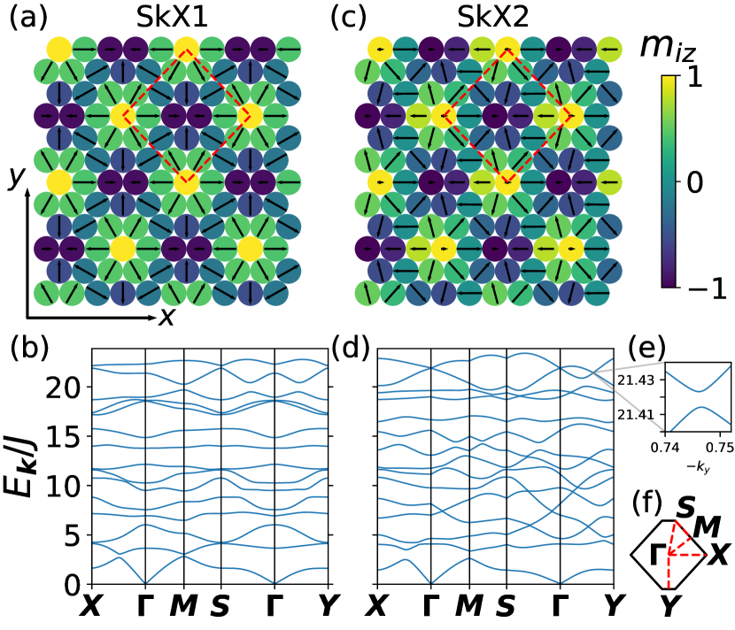
By tuning the parameters to and the GS is a SkX with a periodicity of five lattice sites in the direction and six chains in the direction, at least in the region of easy-axis anisotropy. This is the same periodicity as the best commensurate approximation to the SkX observed in Ref. [18]. We find a quantum phase transition (QPT) between two distinct SkX states with the same periodicity, named SkX1 and SkX2. The QPT occurs at a transition point , where , which is determined by the classical GS energy of the two phases. SkX1 is shown for in Fig. 1(a), while SkX2 is shown for in Fig. 1(c). They are separated by the location of the center of the skyrmion, which is placed exactly at a specific lattice site in SkX1, but has moved approximately one quarter lattice constant to the left of a specific lattice site in SkX2. Ref. [19] also found that the center of the skyrmion relocated when tuning a parameter in the Hamiltonian, there in response to an increasing magnetic field. Here, the center relocates due to stronger easy-axis anisotropy, since the DMI and easy-axis anisotropy terms favor SkX2, while the exchange and four-spin interaction terms favor SkX1.
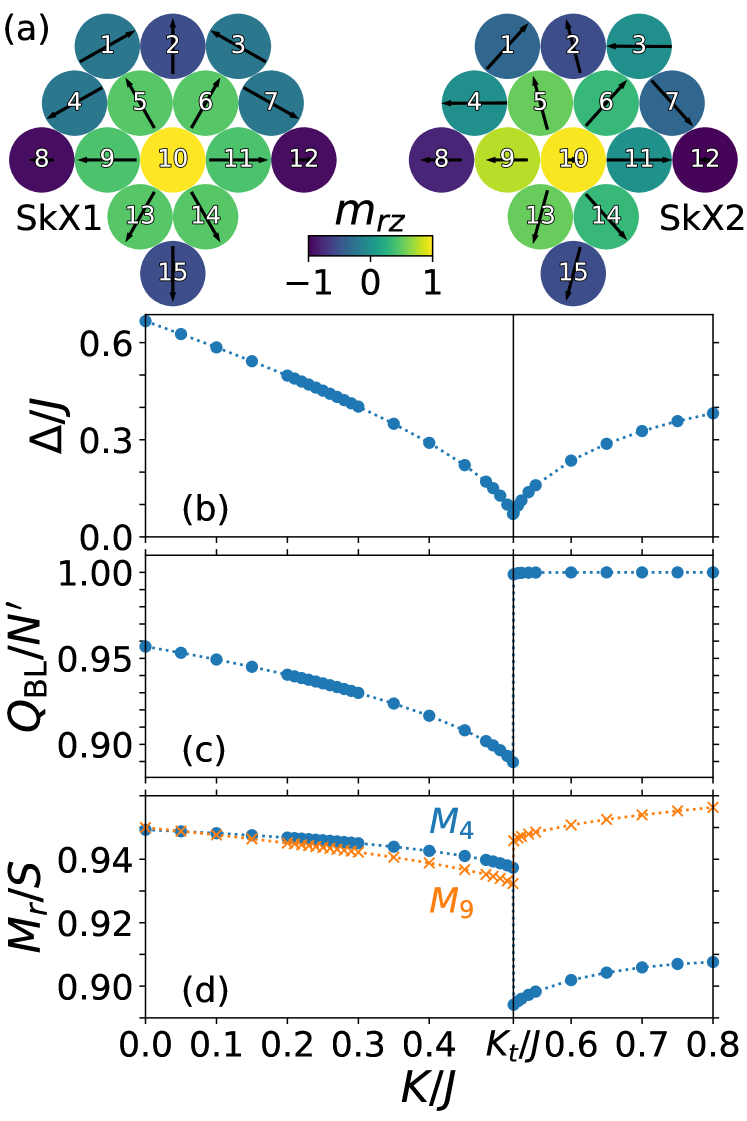
Each phase appears very similar at all considered , except that the absolute value of the component of all spins increases with increasing . For both phases, the magnetic unit cell consists of 15 lattice sites hosting one skyrmion, see Fig. 2(a). This is nearing the lower limit of skyrmion size on a triangular lattice [19, 9, 21]. The Hamiltonian in Eq. (1) is symmetric under spin inversion, i.e., time-reversal symmetric, so states with all spins flipped compared to those in Fig. 1(a,c) are degenerate in energy. Additionally, SkX2 is degenerate with a state where the center relocates by the same length to the right. If these SkXs were created by cooling down an unordered magnetic state in a suitable material, domain walls would probably appear between the degenerate states [18, 33].
A sizable value of is needed in our model to stabilize the quantum skyrmions. DMI originates from spin-orbit coupling (SOC), which is a relativistic effect, and therefore is usually much smaller than in real materials [31, 34, 2]. However, methods of tuning the value of using external lasers [7, 8], even to the point of an exchange free magnet [9], have recently been put forth. Therefore, studying materials with in the laboratory has become feasible. Additionally, in the material in Ref. [18], the large nuclear number of Ir leads to a strong SOC and therefore enhances the DMI. Moreover, the nearest-neighbor exchange interaction is unusually weak due to the strong hybridization of Fe and Ir, which is also why the four-spin interaction is not negligible [18]. While our parameter set differs from that given in Ref. [18], we are modeling a similar material, namely a ferromagnetic monolayer on the surface of a heavy metal which gives rise to strong SOC and a weak nearest-neighbor exchange interaction [18, 2]. However, achieving in a real material still might require tuning [8] to a lower value.
We also present results as functions of the easy-axis anisotropy. Ordinarily, this is considered to be a constant value due to the magnetocrystalline anisotropy in a given material [18, 23, 24, 25]. Therefore one would need to look at different materials in order to observe the changes in the results. However, a method to tune the value of in a material by applying mechanical strain, even managing to change its sign and so change its nature to an easy-plane anisotropy, has recently been discovered [35, 36]. Motivated by this, we will discuss a tunable easy-axis anisotropy . Since the phase transition between SkX1 and SkX2 occurs at zero temperature by tuning a parameter in the Hamiltonian, we identify it as a QPT.
III Magnon description
Ref. [37] introduces a method of performing the HP transformation in noncollinear magnetic ground states. For each lattice site the approach introduces rotated coordinates through an orthonormal frame with . Here, is a unit vector along the spin at lattice site in the classical GS. Furthermore, and . The HP transformation is then introduced as , , , and . Assuming small spin fluctuations, we truncate at second order in magnon operators and therefore neglect magnon-magnon interactions [37, 26]. The assumption of small spin fluctuations should be valid at low temperatures compared to the lowest magnon energy, see Appendix C.
Let be the number of lattice sites and the number of magnetic unit cells. The Fourier transform (FT) is introduced as , assuming lattice site is located on sublattice . The sum over momenta covers the first Brillouin zone (1BZ) of sublattice .
The magnon-independent terms, , correspond to the classical Hamiltonian. It can be shown that linear terms in magnon operators vanish when expanding around the GS [37]. The quadratic terms may be written
| (6) |
where and
| (7) |
The matrix elements are expressed as
| (8) |
| (9) |
| (10) |
| (11) |
| (12) |
Here, is the shortest vector connecting a site on sublattice to a site on sublattice . and if there exist sites such that and are nearest neighbors. Otherwise and . if there exist sites such that make a counterclockwise diamond of minimal area. Otherwise . Since the orthonormal frame is equal for any it is replaced by to facilitate the FT.
IV Magnon spectra
Diagonalizing [38] and applying a bosonic commutator gives
| (13) |
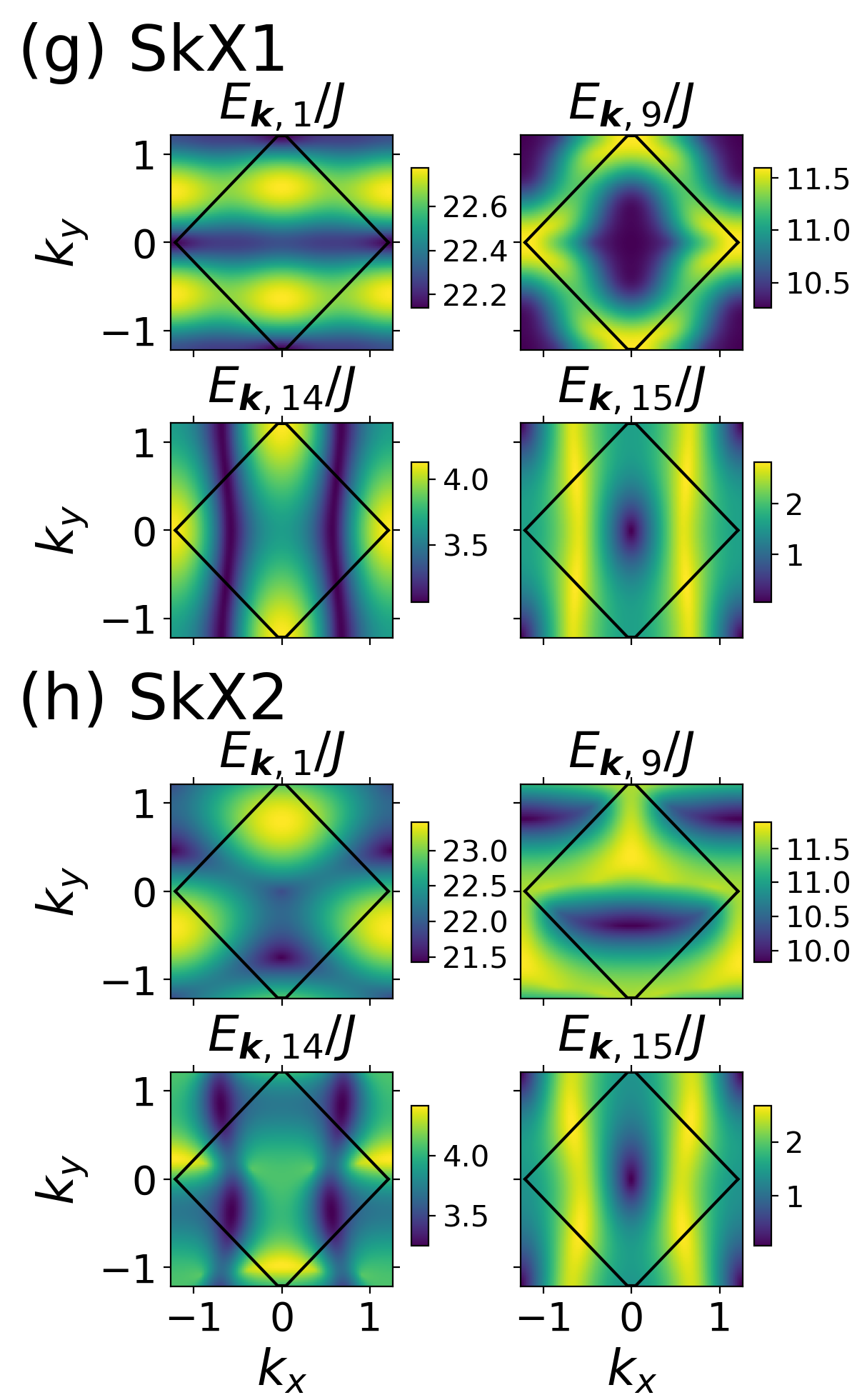
The 15 energy bands are numbered from top to bottom, and plotted for a path in the 1BZ in Fig. 1(b,d). The definition of the points in the 1BZ and its precise structure are given in Appendix A. The number of bands corresponds to the number of sublattices in the GS. A selection of magnon energies are shown in the full 1BZ in Fig. 1(g,h). Possible experimental techniques to measure these collective excitations include spin-resolved electron-energy-loss spectroscopy [25], neutron scattering, and Brillouin light scattering [4]. Compared to earlier studies of SkX magnon spectra [23, 24, 26, 27, 25], our results offer new insight into their behavior in zero external magnetic field.
Note the significant difference between the magnon spectrum of SkX1 in Fig. 1(b,g) compared to that of SkX2 in Fig. 1(d,h). A striking difference is that in SkX1 the energy spectrum obeys , while in SkX2 . The lower symmetry of the magnon spectrum is attributed to the lower symmetry of the GS. The lower symmetry of SkX2 compared to SkX1 is also what clearly identifies it as a separate phase. Both the SkX1 GS and the SkX2 GS show a symmetry under combined real space mirror operation about the plane and spin inversion. Meanwhile, only SkX1 shows symmetry under combined mirror operation about the plane and spin inversion. In both states, for any nearest-neighbor spins and with nearest-neighbor vector , there exists a pair and with nearest-neighbor vector . By inspecting the matrix elements and applying theory concerning the diagonalization method [38, 39], this can be used to show that the matrices and defined in Eq. (7) give the same energy eigenvalues. Hence, symmetry under combined mirror operation about the plane and spin inversion leads to mirror symmetry about the plane for the magnon spectrum. The broken symmetry under combined mirror operation about the plane and spin inversion in SkX2 leads to a broken mirror symmetry about the plane for its magnon spectrum, unlike SkX1.
For SkX1, the magnon gap at the point, , is caused by a combination of the easy-axis anisotropy and the DMI. and involve inner products of spins, and are independent of a global rotation of all spins. Therefore, they should not cause a gap at the point. and protect the GS from a global rotation of all spins, i.e., they break continuous rotational symmetry [26], and therefore they both contribute to the gap at the point. Fig. 2(b) shows how the gap changes when is tuned. Unlike ferro- and antiferromagnets, the gap decreases when the easy-axis anisotropy is increased in the SkX1 phase. For SkX2, the magnon gap has moved slightly away from the point toward positive . We attribute this to the lower symmetry of the SkX2 state. Interestingly, the gap becomes an increasing function of in the SkX2 phase. This further illustrates the difference between the SkX1 and SkX2 phases, and lies at the heart of why the system transitions to the new phase at strong easy-axis anisotropy, see Appendix A. Apart from the dependence of the magnon gap on and a finite number of values where two bands cross [40], the magnon spectrum in each phase is very similar at all considered values of .
V Quantum skyrmion order parameter
The topological skyrmion number counts the number of times the magnetization wraps the unit sphere [1]. It relies on a continuum description, and is inherently classical. A discretized version of the skyrmion number is introduced in Ref. [28] as the total solid angle spanned by the spins, divided by the solid angle of a sphere, . In Ref. [20], the spin products are replaced by correlation functions to obtain a quantum mechanical analog of the topological invariant [19, 20]. The expression is here adapted to general and we use the function to get the correct value of the solid angle for all possible combinations of three spins [41]. The quantum skyrmion OP is
| (14) |
where and . The sum is taken over all nonequivalent triangles of nearest neighbors, oriented counterclockwise [20]. When treating a discrete system of quantum spins, is analogous to the topological invariant of the corresponding classical GS. However, since it is no longer topological in a rigorous sense [19], we name it the quantum skyrmion OP.
For the two SkXs in Fig. 1(a,c) the classical value is an integer per magnetic unit cell, . The value confirms the presence of one skyrmion in the magnetic unit cell. For the degenerate states with all spins flipped compared to SkX1 and SkX2, . Since its sign does not distinguish skyrmions and antiskyrmions, it makes most sense to discuss the absolute value of . We choose to work exclusively with the SkXs that have in this paper. To avoid any confusion in the following we will not put absolute values on the quantum skyrmion OP.
The aim of this paper is to go beyond the classical, integer-valued for the skyrmion OP. In Ref. [19], they defined the quantum scalar chirality as an approximation to , and considered its utility as a quantum skyrmion OP. Within the HP approach, the quantum scalar chirality would be . The phases SkX1 and SkX2 contain triangles where and , and therefore the quantum scalar chirality is a poor approximation to in these SkXs. In the HP approach we can calculate the quantum fluctuations in directly, and then check whether is a good OP for quantum skyrmions.
After inserting the HP transformation to second order in magnon operators, we write and . The terms to zeroth order in magnon operators are the classical values. The expectation values of the linear terms vanish in the diagonalized frame, and so . The quadratic parts are
| (15) |
where H.c. denotes the Hermitian conjugate of the preceding term, and
| (16) |
It is assumed that and to introduce the FT in these expressions. Simultaneously, the sum over sites is replaced by a sum over sublattices , including periodic boundary conditions (PBCs) [42], times the number of magnetic unit cells. To calculate the expectation values, the transformation matrix in Eq. (19) is used to transform to the diagonal basis. Focusing on quantum fluctuations, the temperature is set to zero. Then, the only contribution comes from the commutator in the terms , where at zero temperature. All other operator combinations give zero expectation value in the diagonalized basis. An example of a FT is . Only contributes to the expectation value, and so we get a factor . For more details of how the expectation values are calculated, see Appendix B.
We calculate the expectation values and for the 30 nonequivalent triangles involving nearest-neighbor sites at sublattices , and then insert these in . The results for are shown in Fig. 2(c) as a function of the easy-axis anisotropy . We see that remains clearly nonzero, and so is a good quantum skyrmion OP. It is evident that the quantum fluctuations do not destroy the skyrmion nature of the GS. The jump in at the transition point shows that it is also a good OP for the QPT between two quantum skyrmion phases, SkX1 and SkX2. This is in contrast to the classical version which is the same in both phases. The jump in the OP indicates that the transition between SkX1 and SkX2 is a discontinuous QPT and not a quantum critical phenomenon.
In SkX2, approaches 1 from below with increasing , indicating that the quantum fluctuations in SkX2 barely affect its skyrmion nature. SkX1 contains four triangles in the magnetic unit cell where , while SkX2 contains only two such triangles. In reference to the sublattice numbering in Fig. 2(a) an example of a triangle with that applies to both phases is . In SkX1 at we find that , , , and in these triangles. Hence, the quantum fluctuations have a significant effect on their contribution to the total solid angle. Meanwhile, in SkX2, there are two triangles where , , , and for . Therefore, the quantum fluctuations have a negligible effect on their contribution to the total solid angle. While there are 30 triangles contributing to , we suggest this difference in the subset of triangles with explains the much smaller effect of quantum fluctuations on the quantum skyrmion OP in SkX2 compared to SkX1.
The quantum fluctuations in the OP, i.e., the deviation of from the classical value , increases with decreasing magnon gap, see Fig. 2(b,c). This is understood from the fact that quantum fluctuations become less energetically costly with lower magnon gap. In Fig. 2 we employ a higher density of values between and because there are interesting topological magnon features in this region [40]. We find that these features do not affect the quantum fluctuations. A higher density is also used around where the gap and the fluctuations change more rapidly as functions of . It is emphasized that new GSs are found at each value of .
The classical version, , is zero for all coplanar states, except for a set of exceptional states where three neighboring spins give and . As pointed out in Ref. [28], is not defined in such a case because the sign of the spanned solid angle of is ambiguous. If one considers a system where such exceptional states are possible, one would need to consider whether such coplanar states are special cases of skyrmions, or, adjust the definition of so that all possible coplanar states give . Our results indicate that the fluctuations always have smaller absolute values than the classical values , even when . Hence, a coplanar state which has , will likely give also when including quantum fluctuations. Therefore, should in general be a good OP for the existence of quantum skyrmions.
Probing in an experiment could involve measuring the spin correlation functions in Eq. (14). The spin-spin correlation functions in can be measured by neutron scattering [43, 44] or magnetostriction experiments [45]. Information about the FT of the three-spin correlation function , also referred to as the scalar spin chirality, can be extracted for very small momenta using Raman scattering [46, 47]. Proposals to access information about the FT of the scalar spin chirality at finite momenta include neutron scattering [48] and resonant inelastic x-ray scattering [49].
VI Magnetization
We define the magnetization of sublattice as
| (17) |
In SkX1 we find the strongest quantum fluctuations for the two sublattices to the left and to the right of the central up spin. In our chosen numbering these are sublattices and , see Fig. 2(a). In SkX2 sublattices and show the strongest quantum fluctuations. We show and as functions of for both phases in Fig. 2(d). We see that the corrections to the classical value are less than , supporting the validity of the HP approach. Again, we see that the fluctuations increase with decreasing gap. The spins at sublattice 10 show the weakest quantum fluctuations in both phases, which remain less than for all considered .
VII Conclusion
We studied a weakly exchange-coupled magnetic monolayer where the Dzyaloshinskii-Moriya interaction and the four-spin interaction conspire to create a dense skyrmion crystal. A quantum phase transition between two distinct skyrmion crystals, driven by a tunable easy-axis anisotropy, was found. The magnon spectrum was derived and discussed for both quantum skyrmion phases. The discrete and quantum natures of small skyrmions are not negligible, and hence the continuum and classical topological invariant is rendered ill-defined. We proceeded to study the quantum fluctuations in the discretized order parameter of quantum skyrmions. The order parameter proved to be a good indicator of the presence of quantum skyrmions. Furthermore, it managed to capture the quantum phase transition between distinct skyrmion phases, signaled by a jump in the order parameter at a particular value of the easy-axis anisotropy. It was found that quantum fluctuations do not adversely affect the skyrmion nature of quantum skyrmions compared to their classical ground states.
Acknowledgments
We acknowledge funding from the Research Council of Norway through its Centres of Excellence funding scheme, Project No. 262633, “QuSpin,” and through Project No. 323766, “Equilibrium and out-of-equilibrium quantum phenomena in superconducting hybrids with antiferromagnets and topological insulators.”
Appendix A Ground states
A.1 Periodicity
To obtain the classical GS we replace the spin operators in the Hamiltonian in Eq. (1) by , where is the spin quantum number, and is a unit vector determining the direction of the spin at lattice site . The GS is then the set which minimizes . A challenge is that the periodicity of potential SkXs is a priori unknown, and so any calculation involving a finite number of lattice sites with PBCs will suffer from finite-size effects. We therefore first determine the parameters which give a SkX with the desired periodicity, before finding the best state with that periodicity.
The approach starts from the SkX construction detailed in the supplementary material of Ref. [18]. Among the SkX states covered there, the one which gives the lowest energy in our model is used as a trial state and named SkXt. SkXt is constructed using and . Here is the periodicity in the direction in units of the lattice constant, while is the periodicity in the direction in units of lattice constants. SkXt arranges skyrmions in a centered rectangular lattice. The periodicities and used to specify the GS refer to the conventional unit cell of the centered rectangular lattice, which contains two skyrmions here. It is possible to consider any rational values of and and still make finite-sized lattices with correct PBCs.
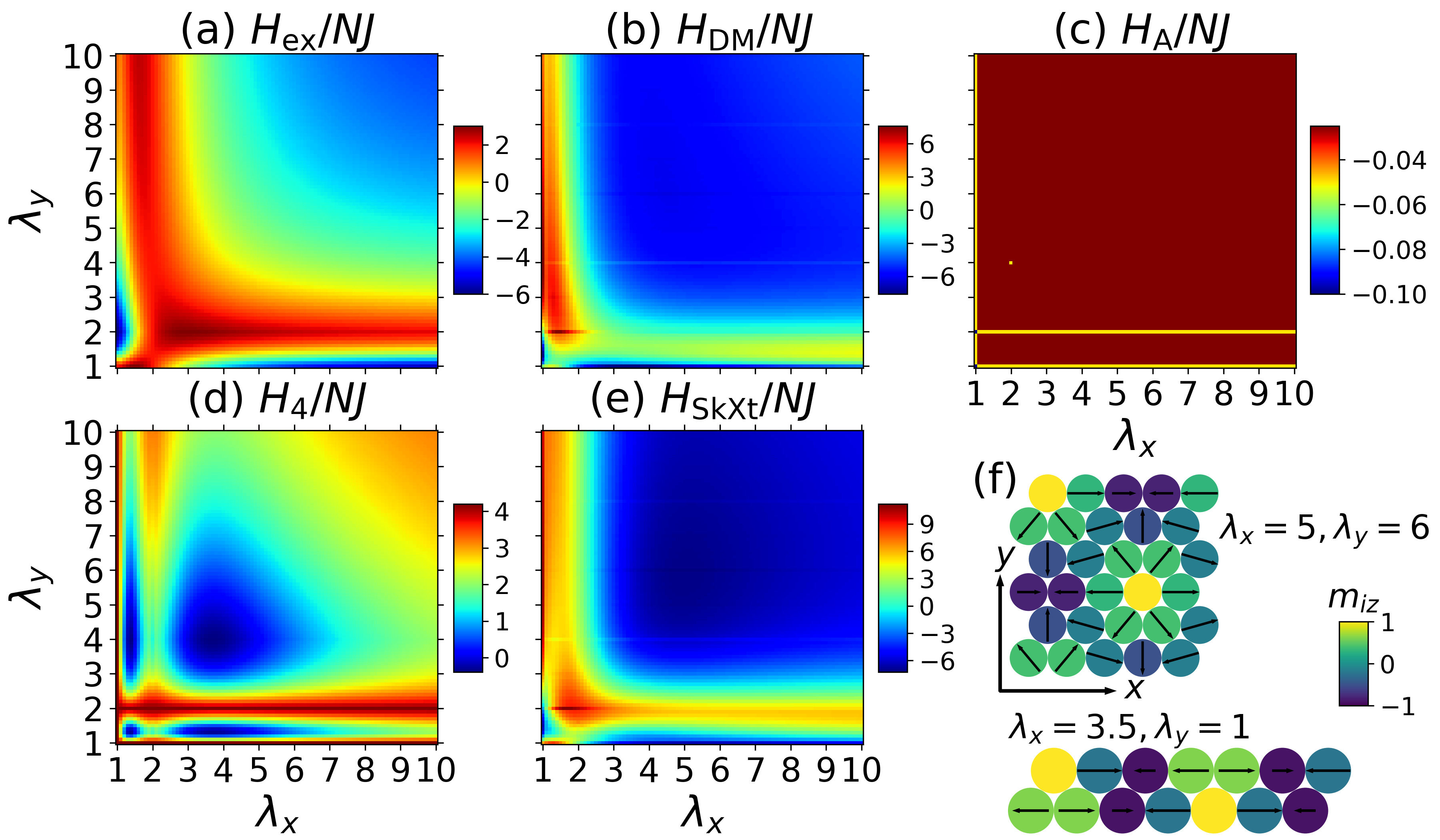
Fig. 3 shows the four individual contributions, as well as the total classical Hamiltonian for SkXt. The exchange and easy-axis anisotropy terms, see Fig. 3(a,c), prefer a ferromagnetic GS, which is achieved with . Special values and general , as well as or and general , give helical states. Some of these are favored by the DMI contribution, see Fig. 3(b), while all are disfavored by the four-spin interaction, see Fig. 3(d). In addition, gives a coplanar state, which, along with the helical states (also coplanar), yields a lower compared to the noncoplanar skyrmion-like states, see Fig. 3(c). Among the possible SkXt states, the DMI term prefers a helical state with . Fig. 3(f) shows the similar helical state with .
When focusing on SkXt states, it is clear that the value of the easy-axis anisotropy has no effect on the periodicity unless it is the dominant energy in the system. However, the true GS will adjust the components of its spins to take advantage of an increased . We kept in the region in this paper and ensured that it did not affect the periodicity of the GS. The total classical Hamiltonian for SkXt states, see Fig. 3(e), is minimized for at and , and that SkXt state is shown in Fig. 3(f). To be specific, we tuned the parameters to ensure that minimizes the total energy of SkXt. This also shows how must be tuned to get the same GS if one considers different . We have set and in this paper.
A.2 Obtaining the ground states
We employ two methods of searching for the GSs, namely Monte Carlo simulated annealing [50, 51, 52, 53, 54, 33, 55, 26, 27] and self-consistent iteration [25, 23, 24]. We obtained the lowest-energy states using the iterative approach, and therefore explain it in detail here. Knowing the periodicity, we can work with the 15-site magnetic unit cell with PBCs [42], see Fig. 2(a) and compare to Fig. 1(a,c). The magnetization on each site is set to , where the inclination and the azimuth are the familiar angles in spherical coordinates. We start from both a random set of angles and the trial state SkXt. Let be the number of iterations completed. Then, for each spin the magnetic torques, and , are calculated. These are used to set new angles and where is the mixing parameter [25]. We used and . The iterations are repeated until self-consistency is reached.
At the end result is the SkX1 state shown in Fig. 1(a), while at the end result is the SkX2 state shown in Fig. 1(c). We emphasize that the SkXs we find as GSs have lower energy than the trial states SkXt used to determine the periodicity. The 15 sublattices in the GSs are equal, centered rectangular lattices with primitive vectors and . Their 1BZ is a nonregular hexagon with vertices at and . We define the points , , , , and in the 1BZ, as shown in Fig. 1(f).
We performed several checks on the proposed GSs. Starting from random states on larger lattices and using Monte Carlo did not yield any states with lower energy. More convincingly, it can be shown that requiring the coefficients of linear terms in the Hamiltonian to be zero, is equivalent to requiring that the zero-order terms are in an extremum, . By calculating the coefficients of the linear terms from the proposed GSs, we get zero within numerical accuracy.
In the numerics, we set so that all quantities are dimensionless. In the numerical GSs obtained with 15 free spins in the magnetic unit cell, the spins show small, , deviations from the symmetries discussed in Sec. IV. By requiring these apparent symmetries to be exact, we find alternative GSs with the same energy to . These small deviations from the apparent symmetries of the classical GSs are therefore viewed as numerical artifacts, which have minor effects on the results. The maximum absolute values of the coefficients of linear terms in the Hamiltonian are due to these artifacts, while exactly symmetric GSs give coefficients of linear terms. All numerical results presented in this paper are accurate down to or better. Achieving accuracy down to should be possible by requiring the numerical GSs to be exactly symmetric, but the corrections would not be visible in any plots presented here.
A.3 Energy correction and net magnetization
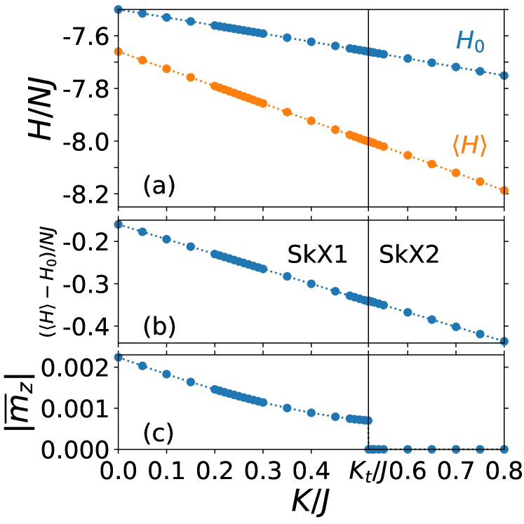
Bosonic commutators were used to write the quadratic terms in the Hamiltonian on the form in Eq. (6), and these yield quantum corrections to the GS energy. Also, the diagonalized in Eq. (13) gives a nonzero contribution at zero temperature, and so the expectation value of the Hamiltonian is
| (18) |
where is the classical GS energy. We plot and in Fig. 4(a). Notice that quantum corrections lower the energy of the skyrmions, which means that quantum fluctuations stabilize skyrmion crystals. Hence, it is the quantum skyrmions, and not the classical GSs, which are the preferred states of the system. This is completely analogous to the HP treatment of antiferromagnets. The same has previously been found for skyrmions in a magnetic field [23, 19]. The plot of in Fig. 4(b) is much closer to being linear than the other plots of quantum fluctuations in Fig. 2. By inspecting the calculated values we find that the magnitude of the slope increases slightly for increasing in both phases. It appears that changes in are dominated by the fact that the Hamiltonian depends linearly on . Also, gradual changes in the GS to take advantage of higher are more important than the value of the magnon gap, since even in SkX2, where the gap is an increasing function of , the magnitude of the slope of increases with .
In the main text, we determined the transition point of the QPT between SkX1 and SkX2 from the classical GS energy . One could also include quantum fluctuations of the energy, and use to determine the transition point. SkX1 remains a local minimum in the classical for , and hence the linear terms in the Hamiltonian remain zero. Therefore, it is possible to use updated versions of SkX1 at and perform calculations of the quantum fluctuations around these states. We then find that also for SkX1 has lower than SkX2. However, at , with , the gap in the magnon spectrum of SkX1 closes. The matrix in Eq. (7) is no longer positive definite for SkX1, and so the method in Ref. [56] must be used to diagonalize the system [38]. This yields complex energy eigenvalues for SkX1 at indicating that SkX1 becomes dynamically unstable [57]. Hence, if determined using rather than , SkX1 is the preferred state up to , at which point a QPT to the dynamically stable SkX2 takes place.
The SkX1 GSs have a small net magnetization, , as opposed to the SkX2 states and the trial SkXt state which have zero net magnetization. The net magnetization is plotted in Fig. 4(c), and it is negative for the SkX1 states with spin up at the center. The Hamiltonian in Eq. (1) does not have Ising symmetry but it would still be natural to assume that the net magnetization of a SkX GS is zero, since there is no external magnetic field. We believe the small net magnetization of SkX1 is simply due to the fact that such a configuration allows a lower total energy from the four competing contributions to the Hamiltonian when placing a dense SkX on the triangular lattice.
Appendix B Diagonalization method
The matrix in Eq. (7) is Hermitian, , while its block elements obey and . is also positive definite in this bosonic system. Therefore, we employ the matrix generalization of the Bogoliubov transformation introduced in Ref. [38] to diagonalize the Hamiltonian. Then, we are guaranteed that the excitation spectrum is real [38], and hence that the system is stable [57]. In Ref. [58], we used the method described in Refs. [56, 39] because the matrix was not positive definite in all phases. We have confirmed that all results in this paper are the same when using either diagonalization method.
The diagonalization [38],
where is diagonal, preserves the bosonic commutator relations for the diagonalized operators . For a system with degrees of freedom, the matrices are of size . In our system, , i.e., the number of sublattices in the GS.
Unlike fermionic systems, the excitation spectrum is not simply the eigenvalues of , and the transformation matrix is paraunitary, [38], rather than unitary. Here, is a diagonal matrix whose first diagonal elements are , and final diagonal elements are . Since is positive definite, its Cholesky decomposition, , exists, where is upper triangular. The algorithm presented in Ref. [38] then proceeds to find orthonormal eigenvectors and eigenvalues of the Hermitian matrix . It can be shown that for , where and . The positive eigenvalues are the excitation spectrum of the system [38]. To complete the diagonalization, the unitary matrix is constructed from the orthonormal eigenvectors and the diagonal matrix is constructed from the eigenvalues . The inverse of the transformation matrix, , is then calculated row by row from starting at the last row.
The transformation matrix can be written
| (19) |
Then, using the transformation to the diagonal basis is given by
| (20) | ||||
| (21) |
From this transformation, we find that at zero temperature
| (22) | ||||
| (23) | ||||
| (24) |
, , and . These are used extensively in the paper to calculate quantum fluctuations.
Appendix C Thermal effects on order parameter
To include thermal fluctuations when calculating expectation values of operator combinations, one also takes into account that
| (25) |
according to Bose-Einstein statistics. Here, is the temperature, and we have set Boltzmann’s constant . As an example,
Table 1(a) shows the results for the quantum skyrmion OP in SkX1 at . There, the magnon gap is . At least when the thermal effects do not adversely affect the utility of in indicating the presence of quantum skyrmions. The conclusion is the same when considering a lower magnon gap in SkX1 in Table 1(b). In fact, it seems thermal fluctuations have a lesser effect when viewed in terms of here. This is due to the fact that the valley around the global minimum of is sharper at than at . Like the quantum fluctuations, SkX2 is also less affected by thermal fluctuations compared to SkX1, see Table 1(c). We suggest the reason is the same as that given when discussing the quantum fluctuations in Sec. V. If the weak exchange coupling is meV, then the temperatures considered in Table 1 correspond to K.
| (a) SkX1, , | ||||||
|---|---|---|---|---|---|---|
| (b) SkX1, , | ||||||
| (c) SkX2, , | ||||||
References
- Nagaosa and Tokura [2013] N. Nagaosa and Y. Tokura, Nat. Nanotechnol. 8, 899 (2013).
- Finocchio et al. [2016] G. Finocchio, F. Büttner, R. Tomasello, M. Carpentieri, and M. Kläui, J. Phys. D: Appl. Phys. 49, 423001 (2016).
- Jonietz et al. [2010] F. Jonietz, S. Mühlbauer, C. Pfleiderer, A. Neubauer, W. Münzer, A. Bauer, T. Adams, R. Georgii, P. Böni, R. A. Duine, K. Everschor, M. Garst, and A. Rosch, Science 330, 1648 (2010).
- Back et al. [2020] C. Back, V. Cros, H. Ebert, K. Everschor-Sitte, A. Fert, M. Garst, T. Ma, S. Mankovsky, T. L. Monchesky, M. Mostovoy, N. Nagaosa, S. S. P. Parkin, C. Pfleiderer, N. Reyren, A. Rosch, Y. Taguchi, Y. Tokura, K. von Bergmann, and J. Zang, J. Phys. D: Appl. Phys. 53, 363001 (2020).
- Tomasello et al. [2014] R. Tomasello, E. Martinez, R. Zivieri, L. Torres, M. Carpentieri, and G. Finocchio, Sci. Rep. 4, 6784 (2014).
- Fert et al. [2013] A. Fert, V. Cros, and J. Sampaio, Nat. Nanotechnol. 8, 152 (2013).
- Mazurenko et al. [2021] V. V. Mazurenko, Y. O. Kvashnin, A. I. Lichtenstein, and M. I. Katsnelson, J. Exp. Theor. Phys. 132, 506 (2021).
- Stepanov et al. [2017] E. A. Stepanov, C. Dutreix, and M. I. Katsnelson, Phys. Rev. Lett. 118, 157201 (2017).
- Stepanov et al. [2019] E. A. Stepanov, S. A. Nikolaev, C. Dutreix, M. I. Katsnelson, and V. V. Mazurenko, J. Phys.: Condens. Matter 31, 17LT01 (2019).
- Romming et al. [2013] N. Romming, C. Hanneken, M. Menzel, J. E. Bickel, B. Wolter, K. von Bergmann, A. Kubetzka, and R. Wiesendanger, Science 341, 636 (2013).
- Hsu et al. [2017] P.-J. Hsu, A. Kubetzka, A. Finco, N. Romming, K. von Bergmann, and R. Wiesendanger, Nat. Nanotechnol. 12, 123 (2017).
- Yu et al. [2017] G. Yu, P. Upadhyaya, Q. Shao, H. Wu, G. Yin, X. Li, C. He, W. Jiang, X. Han, P. K. Amiri, and K. L. Wang, Nano Lett. 17, 261 (2017).
- Je et al. [2020] S.-G. Je, H.-S. Han, S. K. Kim, S. A. Montoya, W. Chao, I.-S. Hong, E. E. Fullerton, K.-S. Lee, K.-J. Lee, M.-Y. Im, and J.-I. Hong, ACS Nano 14, 3251 (2020).
- Parkin et al. [2008] S. S. P. Parkin, M. Hayashi, and L. Thomas, Science 320, 190 (2008).
- Zhang et al. [2015] X. Zhang, M. Ezawa, and Y. Zhou, Sci. Rep. 5, 9400 (2015).
- Psaroudaki and Panagopoulos [2021] C. Psaroudaki and C. Panagopoulos, Phys. Rev. Lett. 127, 067201 (2021).
- Mühlbauer et al. [2009] S. Mühlbauer, B. Binz, F. Jonietz, C. Pfleiderer, A. Rosch, A. Neubauer, R. Georgii, and P. Böni, Science 323, 915 (2009).
- Heinze et al. [2011] S. Heinze, K. von Bergmann, M. Menzel, J. Brede, A. Kubetzka, R. Wiesendanger, G. Bihlmayer, and S. Blügel, Nat. Phys. 7, 713 (2011).
- Sotnikov et al. [2021] O. M. Sotnikov, V. V. Mazurenko, J. Colbois, F. Mila, M. I. Katsnelson, and E. A. Stepanov, Phys. Rev. B 103, L060404 (2021).
- Lohani et al. [2019] V. Lohani, C. Hickey, J. Masell, and A. Rosch, Phys. Rev. X 9, 041063 (2019).
- Gauyacq and Lorente [2019] J.-P. Gauyacq and N. Lorente, J. Condens. Matter Phys. 31, 335001 (2019).
- Ochoa and Tserkovnyak [2019] H. Ochoa and Y. Tserkovnyak, Int. J. Mod. Phys. B 33, 1930005 (2019).
- Roldán-Molina et al. [2015] A. Roldán-Molina, M. J. Santander, A. S. Nunez, and J. Fernández-Rossier, Phys. Rev. B 92, 245436 (2015).
- Roldán-Molina et al. [2016] A. Roldán-Molina, A. S. Nunez, and J. Fernández-Rossier, New J. Phys. 18, 045015 (2016).
- dos Santos et al. [2018] F. J. dos Santos, M. dos Santos Dias, F. S. M. Guimarães, J. Bouaziz, and S. Lounis, Phys. Rev. B 97, 024431 (2018).
- Díaz et al. [2019] S. A. Díaz, J. Klinovaja, and D. Loss, Phys. Rev. Lett. 122, 187203 (2019).
- Díaz et al. [2020] S. A. Díaz, T. Hirosawa, J. Klinovaja, and D. Loss, Phys. Rev. Res. 2, 013231 (2020).
- Berg and Lüscher [1981] B. Berg and M. Lüscher, Nucl. Phys. B. 190, 412 (1981).
- Holstein and Primakoff [1940] T. Holstein and H. Primakoff, Phys. Rev. 58, 1098 (1940).
- Dzyaloshinsky [1958] I. Dzyaloshinsky, J. Phys. Chem. Solids 4, 241 (1958).
- Moriya [1960] T. Moriya, Phys. Rev. 120, 91 (1960).
- MacDonald et al. [1988] A. H. MacDonald, S. M. Girvin, and D. Yoshioka, Phys. Rev. B 37, 9753 (1988).
- Hagemeister et al. [2016] J. Hagemeister, D. Iaia, E. Y. Vedmedenko, K. von Bergmann, A. Kubetzka, and R. Wiesendanger, Phys. Rev. Lett. 117, 207202 (2016).
- Zhang et al. [2021] H. Zhang, C. Xu, C. Carnahan, M. Sretenovic, N. Suri, D. Xiao, and X. Ke, Phys. Rev. Lett. 127, 247202 (2021).
- Webster and Yan [2018] L. Webster and J.-A. Yan, Phys. Rev. B 98, 144411 (2018).
- Albaridy et al. [2020] R. Albaridy, A. Manchon, and U. Schwingenschlögl, J. Condens. Matter Phys. 32, 355702 (2020).
- Haraldsen and Fishman [2009] J. T. Haraldsen and R. S. Fishman, J. Condens. Matter Phys. 21, 216001 (2009).
- Colpa [1978] J. H. P. Colpa, Phys. A: Stat. Mech. Appl. 93, 327 (1978).
- Xiao [2009] M.-w. Xiao, arXiv:0908.0787 (2009).
- Mæland and Sudbø [2022] K. Mæland and A. Sudbø, arXiv:2205.12965 (2022).
- Van Oosterom and Strackee [1983] A. Van Oosterom and J. Strackee, IEEE. Trans. Biomed. BME-30, 125 (1983).
- Sausset and Tarjus [2007] F. Sausset and G. Tarjus, J. Phys. A: Math. Theor. 40, 12873 (2007).
- Marshall and Lowde [1968] W. Marshall and R. D. Lowde, Rep. Prog. Phys. 31, 705 (1968).
- Shirane et al. [1987] G. Shirane, Y. Endoh, R. J. Birgeneau, M. A. Kastner, Y. Hidaka, M. Oda, M. Suzuki, and T. Murakami, Phys. Rev. Lett. 59, 1613 (1987).
- Zapf et al. [2008] V. S. Zapf, V. F. Correa, P. Sengupta, C. D. Batista, M. Tsukamoto, N. Kawashima, P. Egan, C. Pantea, A. Migliori, J. B. Betts, M. Jaime, and A. Paduan-Filho, Phys. Rev. B 77, 020404(R) (2008).
- Shastry and Shraiman [1990] B. S. Shastry and B. I. Shraiman, Phys. Rev. Lett. 65, 1068 (1990).
- Sulewski et al. [1991] P. E. Sulewski, P. A. Fleury, K. B. Lyons, and S-W. Cheong, Phys. Rev. Lett. 67, 3864 (1991).
- Lee and Nagaosa [2013] P. A. Lee and N. Nagaosa, Phys. Rev. B 87, 064423 (2013).
- Ko and Lee [2011] W.-H. Ko and P. A. Lee, Phys. Rev. B 84, 125102 (2011).
- Kirkpatrick et al. [1983] S. Kirkpatrick, C. D. Gelatt, and M. P. Vecchi, Science 220, 671 (1983).
- Okubo et al. [2012] T. Okubo, S. Chung, and H. Kawamura, Phys. Rev. Lett. 108, 017206 (2012).
- Rózsa et al. [2016] L. Rózsa, E. Simon, K. Palotás, L. Udvardi, and L. Szunyogh, Phys. Rev. B 93, 024417 (2016).
- Keesman et al. [2015] R. Keesman, A. O. Leonov, P. van Dieten, S. Buhrandt, G. T. Barkema, L. Fritz, and R. A. Duine, Phys. Rev. B 92, 134405 (2015).
- Siemens et al. [2016] A. Siemens, Y. Zhang, J. Hagemeister, E. Y. Vedmedenko, and R. Wiesendanger, New J. Phys. 18, 045021 (2016).
- Rosales et al. [2015] H. D. Rosales, D. C. Cabra, and P. Pujol, Phys. Rev. B 92, 214439 (2015).
- Tsallis [1978] C. Tsallis, J. Math. Phys. 19, 277 (1978).
- Pethick and Smith [2008] C. J. Pethick and H. Smith, Bose–Einstein Condensation in Dilute Gases (Cambridge University Press, Cambridge, 2008).
- Mæland et al. [2020] K. Mæland, A. T. G. Janssønn, J. H. Rygh, and A. Sudbø, Phys. Rev. A 102, 053318 (2020).