“The Pedestrian next to the Lamppost”
Adaptive Object Graphs for Better Instantaneous Mapping

Abstract

Estimating a semantically segmented bird’s-eye-view (BEV) map from a single image has become a popular technique for autonomous control and navigation. However, they show an increase in localization error with distance from the camera. While such an increase in error is entirely expected – localization is harder at distance – much of the drop in performance can be attributed to the cues used by current texture-based models, in particular, they make heavy use of object-ground intersections (such as shadows) [10], which become increasingly sparse and uncertain for distant objects. In this work, we address these shortcomings in BEV-mapping by learning the spatial relationship between objects in a scene. We propose a graph neural network which predicts BEV objects from a monocular image by spatially reasoning about an object within the context of other objects. Our approach sets a new state-of-the-art in BEV estimation from monocular images across three large-scale datasets, including a 50% relative improvement for objects on nuScenes.

1 Introduction

The ability to generate top-down birds-eye-view maps from images is an important problem in autonomous driving. Overhead maps provide compact representations of a scene’s spatial configuration and other agents, making it an ideal representation for downstream tasks such as navigation and planning. Given their utility, the BEV estimation problem of inferring semantic BEV maps from images, has drawn increasing attention in recent years — mapping ‘things’ such as traffic cones and pedestrians, and ‘stuff’ such as road lanes and pavements.

Current BEV estimation techniques [34, 37, 36, 32] have made impressive strides towards high-accuracy semantic maps for both ‘things’ and ‘stuff’ from a single image. These texture-based models are elegant in their simplicity, requiring only minimal losses on their predicted BEV maps. Although these models work well for large amorphous textured classes that dominate the scene, such as road and pavement (a.k.a. stuff[4]), they suffer from low recall and large localization error for smaller and potentially dynamic objects at greater distances (a.k.a. things).

In contrast, the field of monocular 3D detection displays far greater object localization accuracy by taking an object-based approach. A simple solution to increase recall and localization accuracy in BEV estimation is to apply an off-the-shelf monocular 3D detector to generate BEV object bounding boxes. Surprisingly, this increases object intersection-over-union (IoU) accuracy on the BEV estimation task by a relative 20%. This raises the question: why not use the best of both methods? That is, reason about objects in object space, and use them to improve the estimates of background ‘stuff’.

We propose a novel BEV estimation method that leverages object graphs to reason about scene layout. These graphs provide a rich source of additional information to improve object localization, as they generate context by propagating between objects. Our model predicts BEV objects from a monocular image by spatially reasoning about an object given the long-range context of other objects in the scene. The contributions of our work are as follows:

1. We propose a novel application of graph convolution networks for spatial reasoning to localize BEV objects from a monocular image.

2. We demonstrate the importance of learning both node and edge embeddings, their mutual enhancement and edge supervision for the problem of object localization.

3. We introduce positional-equivariance into our graph propagation method, leading to state-of-the-art results across three large-scale datasets, including a 50% relative improvement in BEV estimation of ‘things’ or objects.

2 Related Work

BEV Estimation: Initial work in road layout estimation [39] took a two-staged approach of semantic segmentation in the image followed by a homography-based mapping to the ground plane. Others [46, 25, 38] similarly exploited depth and semantic segmentation maps to lift scene and object entities into BEV. As these methods required dense annotation maps as additional input, recent work implicitly reasons about depth and semantics within the network. Some learn image-to-BEV transformations implicitly [27, 28, 31], while more recent approaches improved results by conditioning the transformation on the camera’s geometry [34, 36, 37, 32, 11]. These methods can be broadly categorized by their transformation as either fixed or adaptive. Fixed approaches [34] use a fully-connected layer to vertically condense image features into a bottleneck and then expand into BEV with another fully-connected (FC) layer. One limitation of the approach is that the weights of both FC layers are fixed, increasing the layer’s tendency to ignore small objects and resulting in a low recall for these categories. Adaptive approaches [36, 32] on the other hand, use an attention mechanism that generates context by querying a spatial location. The primary challenge of this approach is the size of the image search space: learning to select the appropriate image features for distant objects whose relevant context is sparse and uncertain is challenging. We overcome the issues with large search spaces by specifically communicating between objects as nodes, aided by scene context sampled along edges.

Monocular Object Detection: In contrast to BEV Estimation, monocular object detection methods are generally object-based, with losses applied per object. Much of this work is centered around constraining the search space — both in the search for objects in the image and their 3D pose regression. A common and successful approach is to constrain the image search space via 2D object detection followed by 3D pose regression [44, 30, 19, 40, 33]. Some approaches use geometric priors to constrain the projected 3D bounding box to fit within the 2D box [30, 14], while others leveraged the relationship between 2D box height and the estimated object height to create initial centroid proposals [23]. Mono3D [6] on the other hand generated 3D proposals on the ground-plane which are then scored by projecting back into the image. The primary drawback of all these methods is that each object proposal is generated independently. Some approaches have tried to reason globally across the scene. OFTNet [35] built on Mono3D to reason globally in BEV by projecting a 3D voxel grid onto the image to collect image-features. However, this creates a bottleneck similar to the fixed BEV-estimators as the features assigned to a voxel are independent of depth. MonoPair [7] constrained the positions of objects by optimizing their pairwise spatial relationships, however this was a post-optimization step outside the network using only the predicted 3D bounding boxes. While graphs have been used for semantic reasoning [48, 9, 26], unlike all previous work, we: (1) use graphs to reason about scene layout and (2) generate context by propagating between objects.

Graph neural networks: Graph neural networks (GNNs) have emerged as a powerful neural architecture to learn from graph-structured data, exhibiting promising results in social networks [29], drug design [41] and more. GNNs build node representations by aggregating local information from their neighborhood. Drawing on the successes of convolutional neural networks (CNNs), several works have generalized convolution operations to the graph domain. These graph convolution networks (GCNs) generally fall into two major categories: spectral and spatial. Spectral approaches [8, 21] perform convolutions in the Fourier domain, while spatial approaches [47, 15] perform them in the node (or vertex) domain. Importantly, our graphs have Euclidean interpretations, thus our graph convolutions need to be spatial instead of spectral. Recently, Velickovic et al. [43] developed an attention-based neighborhood aggregation mechanism operating in the node domain — the Graph Attention Network (GAT). Here, every node updates its representation by attending to its neighbors conditioned on itself, resulting in GATs becoming the state-of-the-art neural architecture for graph learning [2].

Apart from a few notable exceptions [18, 49], most graph learning methods ignore the representational capabilities of edges and focus only on node embeddings. CensNet [18] addressed the utility of edge features by simultaneously embedding both nodes and edges into a latent feature space using spectral graph convolutions. NENN [49] approached this co-embedding in the spatial domain. We similarly learn both node and edge embeddings along with their mutual enhancement. However, unlike all previous approaches, our graph propagation method is made position equivariant to account for the importance of Euclidean structure in localization.

Figure 1: Model Architecture. Our Graph Constructor takes image features $\mathbf{H}^{I}$ and candidate regions $B$ as input and generates a graph $\mathcal{G=(V,E)}$ of the scene’s $N$ objects. The Graph Propagator passes messages across the nodes and edges of the graph in a position-equivariant manner, co-embedding both nodes and edges to a latent feature space for object localisation, resulting in a graph $\mathcal{G^{\prime}=(V^{\prime},E^{\prime})}$ with updated embeddings. The Scene Estimator takes the image features $\mathbf{H}^{I}$ and transforms them to BEV where they are combined with object embeddings $\mathcal{V^{\prime}}$ to generate BEV maps $\mathbf{M}^{BEV}$.

3 Our approach

Given an image captured while driving, we wish to infer a semantically segmented BEV map of its scene. As shown in Fig. 1, we approach BEV estimation as a two stage process of object localization followed by subsequent complete BEV estimation, including the localization of amorphous ’stuff’ such as road or sidewalk that can not be treated as objects. To improve object localization beyond the standard accuracies offered by 3D object detection, we generate context by propagating information between objects to infer their spatial layout. In this section, we first motivate the use of graphs for object localization (Sec. 3.1). We then discuss the main components of our approach shown in Fig. 1: first, we structure scene content in the form of a graph across the image and/or BEV-plane (Sec. 3.2). Next, we localize objects in BEV by propagating structural and positional embeddings across the graph (Sec. 3.4). Finally, we use its learned embeddings to generate complete maps including ‘stuff’ the amorphous regions such as road (Sec. 3.4).

3.1 Design Motivations

Why graph representations? A natural question is what makes object graphs more suitable for localization than current BEV estimation methods? The answer is twofold: (1) graphs encode explicit geometric relationships between objects that BEV networks have to model implicitly and (2) they allow nonlocal communication between entities, which a convolutional BEV network requires many downsampling operations to do. In this section, we build on this to motivate our need for (1) a graph which jointly learns node and edge embeddings; and (2) supervising edge embeddings as a way of placing geometric constraints.

Why learn node embeddings? The primary challenge in object localization is depth estimation. To resolve an object’s depth, monocular scene understanding methods typically rely on visual cues from the object’s intersection with the ground [10]. While artefacts such as shadows provide strong priors, they become increasingly sparse and uncertain for distant objects. When such image features become unreliable, it remains possible to localize an object by comparing its appearance, geometry and position to others in the scene. This can be done by representing each object as a node in a graph and message passing between them.

Why learn edge embeddings? While propagating between nodes provides a baseline mechanism for localization, regressing a node’s location within the graph still requires traversing a large search space. To restrict this space, we can place geometric constraints on object localization by predicting the midpoint of each edge — however, this requires learned edge embeddings.

Figure 2: Our graph propagation method. A single layer of message passing consists of node-to-node and edge-to-node updates, followed by edge-to-edge and node-to-edge updates. The node and edge embeddings of the output graph are then supervised for localisation.

3.2 Graph Construction

Our constructed graphs should represent both scene objects and their spatial relationships. Given an image $\mathbf{I}$ composed of $N$ objects, and with known intrinsic matrix $\mathbf{K}$, our Graph Constructor (shown in Fig. 1) constructs a Euclidean graph $\mathcal{G}=(\mathcal{V},\mathcal{E})$, with $\mathcal{V}$ its set of $N=|\mathcal{V}|$ nodes and $\mathcal{E}$ its set of $E=|\mathcal{E}|$ edges. Each node has explicit Euclidean positional features $p_{i}\in\mathbb{R}^{2}$ representing the object’s estimated location in the ground plane. Aside from its Euclidean representation, each node and edge has a set of image features $S_{i}^{v}$ and $S_{i}^{e}$, respectively.

Unlike the majority of graph-based learning methods where the input graphs are given, we construct ours on the fly. We design our graph based on two key choices: (1) Feature assignment: what features should each node and edge possess? (2) Graph connectivity: how should nodes be connected to each other?

Feature extraction: The features assigned to a node form an initial embedding that is updated in order to make positional predictions in BEV (the same principle also applies to edge embeddings). As described in Sec. 3.1, one way to determine the relative depths of objects in a scene is by comparing their appearance, geometry and position. We represent each of these aspects with the object’s textural features, its 2D bounding box dimensions and its center. Given an image $\mathbf{I}$, we first obtain a set of candidate object regions $B=\{b_{1},...,b_{n}\}$ using a region proposal network. For each region, we obtain its center coordinates $p_{i}^{UV}\in\mathbb{R}^{2}$, its bounding box $b_{i}\in\mathbb{R}^{4}$, and an ROI pooled [13] feature vector $f_{i}\in\mathbb{R}^{C\times h\times w}$. Additionally, for long range vertical context to aid in depth estimation, we include a set of vertical scanlines taken across the bounding box’s width which are pooled horizontally to obtain a feature vector $l_{i}\in\mathbb{R}^{C\times H\times 1}$. This gives us a set of objects $O=\{o_{1},...,o_{n}\}$, where $o_{i}=(p_{i},s_{i})$ is an object with a positional coordinate $p_{i}$ and a set of image feature states $S_{i}=\{b_{i},l_{i},f_{i}\}$.

Graph connectivity: A graph’s structure determines how information is propagated between its nodes and edges. Our input objects are detected in the image, however we want to localize them in BEV. When determining the depth of an object, it is typically more helpful to determine this relative to other objects at similar depths rather than at larger depth differences. For instance, when localizing a distant pedestrian, knowing that it is behind a vehicle that is close to the camera is not useful. Instead, we estimate its depth by looking at where it is in relation to other objects at similar depths. From this, we extract two principles for our graph connectivity: (1) we want our graph structure to exist in the Euclidean domain, where we can connect objects in the image or BEV-plane, (2) we want to order objects by a coarse approximation of their relative depths and then connect them to their nearest depth neighbors. We approximate these coarse, unscaled relative depths $Z^{0}=\{z_{i}^{0},...,z_{n}^{0}\}$ as $Z^{0}=\{\mathbf{d}_{i}\cdot\mathbf{c}|i\in N\}$, where $\mathbf{c}$ is the vector from the center bottom edge of the image to its principal point $(u_{0},v_{0})$ and $\mathbf{d}_{i}$ the object’s vector from from its 2D image coordinate $p_{i}^{UV}$ to the principal point. These relative depth approximations are unscaled and very coarse, serving only to distinguish between an object that is obviously far and one that is near. We then use these coarse unscaled approximations $Z^{0}$ to generate the graph’s connectivity based on nearest neighbors, resulting in an adjacency matrix $A\in\mathbb{R}^{N\times N}$ where $A_{ij}=1$ if there exists an edge between nodes $i$ and $j$.

Embedding initialization: With the graph’s structure determined, we assign its nodes and edges initial features which will be used for propagation later. Below, we describe the features assigned to each node followed by edges.

First, we obtain Euclidean representations $p_{i}^{BEV}\in\mathbb{R}^{2}$ of each node. For each object, we define its initial BEV Euclidean position as $p_{i}^{BEV}=(z_{i}^{0}tan^{-1}(\alpha_{i}^{0}),z_{i}^{0})$, where $\alpha_{i}^{0}$ is its estimated viewing angle. Again, the scale of both parameters is arbitrary and only serves to indicate relative differences between positions. We then define each node’s initial feature as a tuple:

$$\boldsymbol{v}_{i}^{0}=(p_{i},S_{i}=\{b_{i},l_{i},f_{i}\}),$$ (1)

where $p_{i}$ is its BEV coordinate estimate and $S_{i}$ a set of features from the image and BEV.

Then, for each edge’s features $\boldsymbol{e}_{ij}$, we use the adjacency matrix $A$ and follow the same feature extraction process as defined above for the nodes resulting in Eq. 1. Just as each object is defined by a bounding box, we similarly define each edge as its bounding box region in the image. Consequently, the node feature extraction process described above can be applied to each edge.

Finally, we have a graph $\mathcal{G}=(\mathcal{V},\mathcal{E})$ where each node has object features $\boldsymbol{v}_{i}^{0}=(p_{i}^{v},S_{i}^{v}=\{b_{i}^{v},l_{i}^{v},f_{i}^{v}\})$ and each edge has scene features $\boldsymbol{e}_{ij}^{0}=(p_{i}^{e},S_{i}^{e}=\{b_{i}^{e},l_{i}^{e},f_{i}^{e}\})$.

3.3 Graph propagation

Given our input graph $\mathcal{G}$, with initial node features $\boldsymbol{v}_{i}^{0}$ and edge features $\boldsymbol{e}_{ij}^{0}$, we want to pass messages across and between both nodes and edges to learn updated embeddings $\boldsymbol{v}_{i}^{\prime}$ and $\boldsymbol{e}_{ij}^{\prime}$, which we will use for localization. We think of the input graph as a perturbed mass and spring system, and the message passing as a relaxation process that returns the system to equilibrium, which in our case would be the output object locations. Our message passing mechanism, illustrated in Fig. 2, is motivated by the challenges posed by standard GNNs: namely, (1) the need for spatial awareness, or more explicitly, positional equivariance and (2) mutually enhanced node and edge embeddings.

Positional equivariance: To describe how we build positional equivariance into our graph propagation, we begin with the standard GCN formulation and the challenges it poses for our task. We then formulate our approach in response to those challenges.

Given a graph $\mathcal{G}=(\mathcal{V},\mathcal{E})$, a standard GCN layer takes as input a set of node embeddings $\{\boldsymbol{h}_{i}\in\mathbb{R}^{d}|i\in V\}$ and edges $E$. The layer produces an updated set of node embeddings $\{\boldsymbol{h}_{i}^{\prime}\in\mathbb{R}^{d}|i\in V\}$ by applying the same parametric function $f_{W}$ to every node given its neighbors $\mathcal{N}_{i}=\{j\in V|(j,i)\in E\}$:

$$\boldsymbol{h}_{i}^{\prime}=f_{W}(\boldsymbol{h}_{i},\textsc{aggregate}(\{\boldsymbol{h}_{j}|j\in\mathcal{N}_{i}\}))$$ (2)

These graph convolution functions are designed to be invariant to node position and permutation because in most graph learning tasks there is no canonical position for its nodes. Thus, such a function would fail to differentiate isomorphic nodes with the same 1-hop local neighborhood. This is unsuitable for our task, as objects may typically have the same node degree yet have completely different Euclidean structures. To overcome this, we concatenate Euclidean positional information to the node’s features during message passing (Eq. 3). This allows us to learn node representations which capture Euclidean structure. Additionally, the Euclidean structure of our graph changes between successive message passing layers, raising the need for updated positional information at each message passing layer. We do this by propagating positional embeddings to learn better structures at the next update (Eq. 4). This differs from existing GCNs which integrate positional information by concatenating it with the input node features only [12, 1, 22]. Given these requirements, we propose a spatially-aware message-passing mechanism with learnable structural and positional embeddings. The generic update equations of our method are defined as:

$$\begin{split}\boldsymbol{h}_{i}^{\prime}=f_{h}([\boldsymbol{h}_{i}\|\boldsymbol{p}_{i}],\textsc{aggregate}(\{[\boldsymbol{h}_{j}\|\boldsymbol{p}_{j}]|j\in\mathcal{N}_{i}\})),\\ \forall\boldsymbol{h}_{i}\in S_{i}.\end{split}$$ (3)

$$\boldsymbol{p}_{i}^{\prime}=f_{p}(\boldsymbol{p}_{i},\textsc{aggregate}(\{\boldsymbol{p}_{j}|j\in\mathcal{N}_{i}\})),$$ (4)

where $\|$ is the concatenation operation and $f_{h}$ and $f_{p}$ represent separate parametric functions for each feature state in $S_{i}$ and position, respectively. In this way, positional information is updated and dissipated through each feature state at each round of message passing.

Mutually enhanced node and edge embeddings: We wish to learn both node and edge embeddings by propagating information between them. That is, alongside node-to-node and edge-to-edge propagation, we also want edge-to-node and node-to-edge communication. Here we detail the application of our generic update equations (Eq. 3 and 4) to mutually enhance node and edge embeddings. As shown in Fig. 2, each round of message passing consists of two update mechanisms: a node-level update followed by an edge-level update.

In our node-level update, each node state calculates a weighted average of the node and edge states of its neighborhood. Each node $i$ updates its position $\boldsymbol{p}_{i}^{v}$ and its feature states $\boldsymbol{x}_{i}^{v}\in S_{i}^{v}$ by computing a weighted average of the corresponding states of its neighborhood’s nodes $\boldsymbol{x}_{j}^{v}\in S_{j}^{v}$ and edges $\boldsymbol{x}_{ij}^{e}\in S_{ij}^{e}$:

$$\begin{split}\boldsymbol{x}^{v\prime}_{i}=\alpha_{i,i}\boldsymbol{\Theta}_{x}[\boldsymbol{x}_{i}^{v}\|\boldsymbol{p}_{i}^{v}]+\sum_{j\in\mathcal{N}(i)}\alpha_{i,j}\boldsymbol{\Theta}_{x}([\boldsymbol{x}_{j}^{v}\|\boldsymbol{p}_{j}^{v}]+[\boldsymbol{x}_{ij}^{e}\|\boldsymbol{p}_{ij}^{e}]),\\ \boldsymbol{x}_{i}^{v},\boldsymbol{p}_{i}^{v},\boldsymbol{x}_{ij}^{e},\boldsymbol{p}_{ij}^{e}\in\mathbb{R}^{d},\boldsymbol{\Theta}_{x}\in\mathbb{R}^{d^{\prime}\times 2d}\end{split}$$ (5)

$$\begin{split}\boldsymbol{p}^{v\prime}_{i}=\alpha_{i,i}\boldsymbol{\Theta}_{p}\boldsymbol{p}_{i}^{v}+\sum_{j\in\mathcal{N}(i)}\alpha_{i,j}\mathbf{\Theta_{p}}(\boldsymbol{p}_{j}^{v}+\boldsymbol{p}_{ij}^{e}),\\ \boldsymbol{p}_{i}^{v},\boldsymbol{p}_{ij}^{e}\in\mathbb{R}^{d},\boldsymbol{\Theta}_{p}\in\mathbb{R}^{d^{\prime}\times d}\end{split}$$ (6)

where $\boldsymbol{\Theta}$ is a linear transformation weight matrix, and $\alpha_{i,j}$ is an attention coefficient which we define below. We have excluded the nonlinearity that is applied to $\boldsymbol{x}_{i}^{v^{\prime}}$ and $\boldsymbol{p}_{i}^{v^{\prime}}$ for clarity. The inclusion of edge embedding $[\boldsymbol{x}_{ij}^{e}\|\boldsymbol{p}_{ij}^{e}]$ makes this equation a node-to-node + edge-to-node update, meaning the updated node embedding contains context from its edge embeddings. If we wanted to keep this purely node-to-node, we would simply omit the edge embeddings.

For our weighted average, we apply attention over the neighborhood similar to GAT [43], however we also include edge embeddings in this calculation. In our approach, each node $i$ calculates the importance of its neighboring node $j$ and the edge between them $e_{ij}$ using a scoring function $\Lambda:\mathbb{R}^{d}\times\mathbb{R}^{d}\times\mathbb{R}^{d}\rightarrow\mathbb{R}$ to calculate the attention coefficients:

$$\begin{split}\Lambda(\boldsymbol{h}_{i},\boldsymbol{h}_{j},\boldsymbol{e}_{i,j})=\sigma(\boldsymbol{a}^{\top}\cdot[\boldsymbol{\Theta}\boldsymbol{h}_{i}\|\boldsymbol{\Theta}\boldsymbol{h}_{j}\|\boldsymbol{\Theta}\boldsymbol{e}_{i,j}]),\\ \boldsymbol{\Theta}\in\mathbb{R}^{d^{\prime}\times d},\boldsymbol{a}\in\mathbb{R}^{3d^{\prime}}\end{split}$$ (7)

where $\boldsymbol{a}$ and $\boldsymbol{\Theta}$ are learned weights and $\sigma$ is a LeakyReLU nonlinearity. Finally, the attention coefficients are normalized across all choices of $j$ using the softmax function:

$$\alpha_{i,j}=\frac{\exp\left(\Lambda(\boldsymbol{h}_{i},\boldsymbol{h}_{j},\boldsymbol{e}_{i,j})\right)}{\sum_{k\in\mathcal{N}(i)\cup\{i\}}\exp\left(\Lambda(\boldsymbol{h}_{i},\boldsymbol{h}_{k},\boldsymbol{e}_{i,k})\right)},$$ (8)

Similarly, our edge-level update aggregates its neighboring edge and node embeddings. However, incorporating node embeddings into the aggregation function is challenging over the input graph $\mathcal{G}$. Instead, we construct its conjugate graph $\phi(\mathcal{G})$ and perform the edge-level updates here. The conjugate, $\phi(\mathcal{G})$, is a graph whose nodes are edges of $\mathcal{G}$ and two nodes are adjacent in $\phi(\mathcal{G})$ if and only if the corresponding edges are adjacent in $\mathcal{G}$. The adjacency matrix $A^{e}$ of the conjugate $\phi(\mathcal{G})$ can be calculated as follows:

$$A^{e}=C^{T}C-2I$$ (9)

where $C$ is the incidence matrix of the input graph $\mathcal{G}$, and $I$ is the identity matrix. Using the conjugate $\phi(\mathcal{G})=(\mathcal{V}_{\phi},\mathcal{E}_{\phi})$, each edge embedding $\{\boldsymbol{e}_{i,j}\in\mathbb{R}^{d}|i\in\mathcal{V}_{\phi}\}$ can be updated using Eq. 5 - 8, except with nodes and edges swapped.

After multiple rounds of message-passing, our graph propagation method outputs a graph with updated node embeddings $\{\boldsymbol{v}_{i}{{}^{\prime}}=(p_{i}^{v}{{}^{\prime}},S_{i}^{v}{{}^{\prime}}=\{b_{i}^{v}{{}^{\prime}},l_{i}^{v}{{}^{\prime}},f_{i}^{v}{{}^{\prime}}\})|i\in\mathcal{V}\}$ and edge embeddings $\{\boldsymbol{e}_{ij}^{\prime}=(p_{i}^{e}{{}^{\prime}},S_{i}^{e}{{}^{\prime}}=\{b_{i}^{e}{{}^{\prime}},l_{i}^{e}{{}^{\prime}},f_{i}^{e}{{}^{\prime}}\})|(i,j)\in\mathcal{E}\}$.

3.4 Scene estimation

Using the node embeddings output by our graph propagation module, we make predictions for scene categories. Here we take a texture-based approach based on [36], where image features from our frontend are transformed into the BEV-plane to generate BEV maps for scene categories. However, one key difference is that we condition the latent features of this module on our node embeddings. In this way, we constrain the latent BEV space for scene categories as objects provide strong cues for the existence of roads, pavements, etc.

Following [36], a Transformer $\mathcal{T}$ [42] maps image features $\mathbf{H}^{I}$ to BEV-features $\mathbf{H}^{BEV}$:

$$\begin{gathered}\mathcal{T}:\mathbb{R}^{C\times H\times W}\times\mathbb{R}^{3\times 3}\rightarrow\mathbb{R}^{C\times 100\times 100}\\ (\mathbf{H}^{I},\mathbf{K})\rightarrow\mathbf{H}^{BEV}.\end{gathered}$$ (10)

A decoder $\mathcal{D}$ with deep layer aggregation [50] then generates BEV maps for scene categories using the latent BEV features $\mathbf{H}^{BEV}$ conditioned on node embeddings $\{\boldsymbol{v}_{i}^{\prime}|i\in\mathcal{V}\}$:

$$\begin{gathered}\mathcal{D}:\mathbb{R}^{C\times 100\times 100}\times\mathbb{R}^{L_{V}}\rightarrow\mathbb{R}^{k\times 100\times 100}\\ (\mathbf{H}^{BEV},\{\boldsymbol{v}_{i}|i\in\mathcal{V}\})\rightarrow\mathbf{M}^{BEV}.\end{gathered}$$ (11)

3.5 Loss

Object Network: Our object network predicts parameters to help recover the object’s BEV-bounding box with its yaw $\theta$, dimensions $\delta=(l,w)$, centroid $p^{v}=(x,z)$ and label $c$. Additionally, we also predict the midpoint of our graph’s edges $p^{e}=(x,z)$. For each of these heads we first apply a two-layer MLP to the appropriate input feature.

Node and Edge localization: We supervise the graph’s output node and edge embeddings $\boldsymbol{v}_{i}^{\prime}$ and $\boldsymbol{e}_{ij}^{\prime}$ entirely for localization. To obtain BEV positions $(x,z)$, we regress parameters for each using separate MLPs. We regress viewing angle $\alpha$ using the viewing angle $\alpha^{0}$ estimated in the Graph Constructor, and directly regress z-axis depth $z$. The viewing angle and z-axis depth are then used to determine $x$.

Classification, Dimensions and Orientation: We use the initialized node features $\boldsymbol{v}_{i}^{0}$ to make predictions for the object’s label, dimensions and orientation. As shown in Fig. 1, these estimations are made early in the network so they constrain the graph’s initial features when used for localization later. For object classification, we use the focal loss [24] in its original formulation. We directly regress object dimensions. Instead of predicting object yaw $\theta$, we predict its observation angle $\beta$, which is the sum of its viewing angle and object yaw. Estimating observation angle rather than yaw helps account for an object’s changing appearance based on its viewing angle [30]. We follow [30] and estimate observation angle using a discrete-continuous loss: the orientation range is discretized into multiple bins and then the angle is regressed as an offset from the bin center.

Our object network is trained using a multitask loss defined as:

$$L_{total}=L_{loc^{v}}+L_{loc^{e}}+L_{\theta}+L_{dim}+L_{c}$$ (12)

where $L_{loc^{v}}$, $L_{loc^{e}}$ and $L_{dim}$ and regression losses for the object’s centroid, edge midpoint, and object dimensions, $L_{\theta}$ is the discrete-continuous loss for orientation, and $L_{c}$ is the object classification loss. All regression losses use the Smooth L1 Loss and all classification losses use a cross-entropy loss unless otherwise specified.

Scene Network: We train our scene network using the same multiscale Dice loss as [36]. Please see the supplementary for further details on all losses.

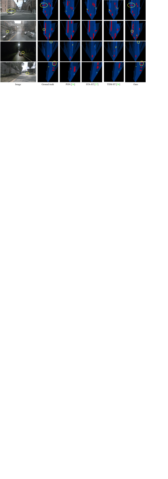
Figure 3: Our model results on nuScenes. As highlighted, our model is able to localize distant and/or heavily occluded vehicles and pedestrians, which the other methods miss.

4 Experiments

Datasets: We compare our approach to current state-of-the-art approaches on the nuScenes [3], Argoverse [5] and Lyft [20] datasets. nuScenes [3] consists of 1000 clips 20-seconds in length, captured across different cities. Each scene is annotated with 3D bounding boxes for 10 object classes, along with vector maps for the road, sidewalk, and more. We generate our BEV ground truth maps following [34].

Implementation: We use a pretrained ResNet-50 [16] with a feature pyramid (FPN) as our frontend. We extract each level of the FPN, interpolate to the same size and add, to obtain a single set of features. To obtain our candidate 2D regions in the image, we use FCOS3D [45] and fine tune it to the appropriate dataset (during training we use jittered ground truth regions). Each node in our graph is connected to its 3 nearest neighbors, and we use 2 layers of message-passing. Our BEV Estimation module uses a BEV latent feature space of 100x100 pixels, with each representing $0.5m^{2}$ in world coordinates. Its largest scale output is 100x100 pixels which we upsample to 200x200 for fair comparison with the literature. We optimize using Adam, with a weight decay of $1e-4$, and a learning rate of $5e{-5}$ which decays by 0.99 every epoch for 50 epochs.

4.1 Ablations

Mutually enhanced embeddings: In Table 1 we demonstrate the effectiveness of using node and edge embeddings, mutually enhancing them, and the effect of their supervision. Beginning with a node-only graph results in the lowest IoU (although this is still higher than current SOTA BEV estimators in Table 3). Adding edge embeddings and then allowing nodes to gather information from them (n2n + e2n) increases IoU slightly. This increase is understandable as each node is now gathering context from both its neighboring objects and its surrounding scene. The largest increase in IoU arrives from edge embeddings communicating between themselves and their supervision (n2n + e2n + e2e). This demonstrates the benefit of using edges to geometrically constrain the spatial layout of the nodes. Finally, combining all types of graph propagation with both node and edge supervision results in the best localization, highlighting the benefits of mutually enhanced embeddings.

Table 1: Graph propagation types. IoU(%) across objects for different graph propagation types on nuScenes. n2n = node-to-node, e2n = edge-to-node, e2e = edge-to-edge and n2e = node-to-edge.

Graph Propagation	Supervision	Objects Mean
n2n	nodes	20.0
n2n + e2n	nodes	21.1
n2n + e2n + e2e	nodes and edges	25.9
n2n + e2n + e2e + n2e	nodes and edges	27.1

Graph node and edge features: In Table 2 we demonstrate the effect of initializing nodes and edges with different feature types. Interestingly, relying solely on appearance results in a baseline IoU of 22.5%. This suggests the model is able to localize objects to a large extent just by comparing their textural features. Part of this result also stems from the scene context aggregated by our frontend’s feature pyramid, meaning the ROI crops of each object contain broader scene context and not just the object’s appearance. This may explain why the inclusion of scanline features do not improve upon this much. In contrast, including the object’s bounding box parameters creates the largest improvement. Since images of urban driving environments display strong regularities in scene structure, knowing where an object is in the image and its image dimensions provides enough information to infer depth coarsely. Finally, modulating each feature type with positional information improves upon this further. This can be explained by the attention mechanism: positional approximations of a node’s neighborhood can signal which may be the most relevant, as it is typically the nearest neighbors which are of most use in terms of context for localisation.

Table 2: IoU (%) effect of graph feature types on nuScenes.

Graph Node and Edge Features	Objects Mean
Appearance	22.5
Appearance, scanline	22.9
Appearance, geometry	26.1
Appearance, geometry, scanline	26.2
Position w. appearance, scanline, geometry	27.1

Table 3: nuScenes IoU (%) results on the validation split of [34]. The last row displays the relative improvement per category over the current state-of-the-art BEV Estimators.

Model	Drivable	Crossing	Walkway	Carpark	Car	Truck	Trailer	Bus	Con.Veh.	Bike	Motorbike	Ped.	Cone	Barrier	Mean	Objects Mean
VPN [31]	58.0	27.3	29.4	12.3	25.5	17.3	16.6	20.0	4.9	4.4	5.6	7.1	4.6	10.8	17.4	11.7
PON [34]	60.4	28.0	31.0	18.4	24.7	16.3	16.6	20.8	12.3	9.4	7.0	8.2	5.7	8.1	19.1	12.9
STA-S [37]	71.1	31.5	32.0	28.0	34.6	18.0	11.4	22.8	10.0	14.6	7.1	7.4	5.8	10.8	21.8	14.3
TIIM-S [36]	72.6	36.3	32.4	30.5	37.4	24.5	15.5	32.5	14.8	15.1	8.1	8.7	7.4	15.1	25.1	17.9
FCOS3D [45]	-	-	-	-	28.6	25.0	20.4	34.2	8.1	11.1	14.6	9.8	9.5	23.9	-	18.6
STA-ST [37]	70.7	31.1	32.4	33.5	36.0	22.8	13.6	29.2	12.1	12.1	8.0	8.6	6.9	14.2	23.7	16.4
TIIM-ST [36]	74.5	36.6	35.9	31.3	39.7	26.3	13.9	32.8	14.2	14.7	7.6	9.5	7.6	14.7	25.7	18.1
Ours	75.9	39.7	37.9	36.8	41.5	38.0	28.8	58.1	23.8	12.2	18.4	11.5	9.0	30.1	33.0	27.1
Rel. improv. (%)	6.4	12.9	21.6	20.0	4.5	44.5	73.2	77.2	60.7	-19.0	127.3	21.5	17.8	99.7	32.4	50.0

Table 4: Argoverse results on the validation split of [34].

Method	Drivable	Veh.	Ped.	L.Veh.	Bike	Bus	Trailer	Motorbike	Mean
VPN [31]	64.9	23.9	6.2	9.7	0.9	3.0	0.4	1.9	13.9
PON [34]	65.4	31.4	7.4	11.1	3.6	11.0	0.7	5.7	17.0
TIIM-S [36]	75.9	35.8	5.7	14.9	3.7	30.2	12.1	2.6	22.6
Ours	78.2	52.1	6.9	23.0	3.1	49.0	23.8	6.9	30.3

Table 5: IoU(%) against ‘adaptive’ approaches on nuScenes canonical validation split and Lyft.

	nuScenes			Lyft
	Driv.	Car	Veh.	Driv.	Car	Veh.
LSS [32]	72.9	32.0	32.0	-	43.1	44.6
FIERY [17]	-	39.9	-	-	-	-
TIIM-S [36]	78.9	39.9	38.9	82.0	45.9	45.4
Ours	81.4	41.7	49.8	84.2	47.4	48.3

Effect of graph node degree: In Table 6 we examine the effect of node degree when constructing our input graphs. Broadly, IoU is inversely proportional to node degree. The progressive decrease in performance is explained by the information available to each node when aggregating its neighborhood: larger node degrees entail more redundancies, and learning to minimize this is increasingly challenging as redundancies in the neighborhood grow.

Table 6: IoU(%) effect of node degree on nuScenes.

Node Degree	0	1	2	3	5	10	15	20+
Objects Mean	20.2	26.2	26.5	27.1	21.1	14.2	11.56	10.3

4.2 Comparison to SOTA

Baselines: We compare against a number of state-of-the-art BEV estimation methods across nuScenes, Argoverse and Lyft datasets. We compare against ‘fixed’ approaches VPN [31], PON [34], STA [37], and ‘adaptive’ approaches LSS [32], FIERY [17] and TIIM [36]. For completeness, we also compare our BEV estimation results on ‘objects’ to those of a state-of-the-art 3D object detector FCOS3D [45].

In Table 3, we demonstrate a 30% relative improvement over the next best performing method TIIM [36], outperforming both its spatial TIIM-S and spatio-temporal TIIM-ST models. In particular, our ‘objects’ classes show a relative increase of 50%, with Motorbikes and Barriers showing a 100% relative gain. Much of this difference can be attributed to our object-based approach to localizing these classes. For fair comparison, we also compare our results on ‘objects’ to another object-based approach: FCOS3D [45]. Here we demonstrate a similar 45% relative improvement across all object classes. With FCOS3D producing object bounding boxes just like we do, the difference in performance here is likely due to our graph-based approach to localization. Our results on Argoverse display similar patterns, where we improve upon the next best performing method TIIM-S [36] by 33%.

In Table 5 we outperform adaptive methods [32, 17, 37] on nuScenes and Lyft. A true comparison on Lyft with LSS [32] is not possible as we were unable to acquire their train/validation split. However, the difference in performance can be attributed to us comparing objects for context, while adaptive approaches rely on scene context.

To obtain a more granular understanding of our method’s performance compared to SOTA, we compare IoU (%) accuracy of ‘objects’ as a function of distance from camera in Fig. 4. Current SOTA BEV-Estimators generally drop in IoU as distance increases. While our method shows a slight drop in IoU between 25-45m, it is broadly maintained along the depth axis. This capability for localizing distant objects can be seen in our qualitative results in Fig. 3, where our model is able to correctly localize objects that are distant and/or heavily occluded, which other methods miss.

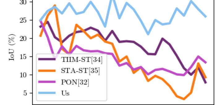
Figure 4: IoU (%) over distance from camera on nuScenes.

4.3 Limitations

Our Graph Constructor enforces many inductive biases, in terms of graph connectivity and feature type . Ideally we want to jointly learn both the connectivity and feature selection while optimizing for object localization. For instance, our IoU on Bikes in Table 3 suggests our graph construction method is not optimal across all object categories. While Bikes are a difficult category due to their large variations in pose, it nonetheless presents an opportunity to learn the graph construction method.

5 Conclusion

We proposed a graph convolution network with a novel position-equivariant message passing mechanism to localize objects in BEV from an image. In particular, we demonstrated the benefit of learning both node and edge embeddings and methods for their mutual enhancement. One of our key insights for better localization is the use of edge features as a method of gathering scene context and its supervision as a way of placing geometric constraints on object locations. Our models are state-of-the-art in BEV estimation from monocular images across three large-scale datasets.

References

- [1] Dominique Beaini, Saro Passaro, Vincent Létourneau, William L. Hamilton, Gabriele Corso, and Pietro Lió. Directional graph networks. In Marina Meila and Tong Zhang, editors, Proceedings of the 38th International Conference on Machine Learning, ICML 2021, 18-24 July 2021, Virtual Event, volume 139 of Proceedings of Machine Learning Research, pages 748–758. PMLR, 2021.
- [2] Michael M Bronstein, Joan Bruna, Taco Cohen, and Petar Veličković. Geometric deep learning: Grids, groups, graphs, geodesics, and gauges. arXiv preprint arXiv:2104.13478, 2021.
- [3] Holger Caesar, Varun Bankiti, Alex H Lang, Sourabh Vora, Venice Erin Liong, Qiang Xu, Anush Krishnan, Yu Pan, Giancarlo Baldan, and Oscar Beijbom. nuscenes: A multimodal dataset for autonomous driving. In Proceedings of the IEEE/CVF Conference on Computer Vision and Pattern Recognition, pages 11621–11631, 2020.
- [4] Holger Caesar, Jasper Uijlings, and Vittorio Ferrari. Coco-stuff: Thing and stuff classes in context. In Proceedings of the IEEE conference on computer vision and pattern recognition, pages 1209–1218, 2018.
- [5] Ming-Fang Chang, John Lambert, Patsorn Sangkloy, Jagjeet Singh, Slawomir Bak, Andrew Hartnett, De Wang, Peter Carr, Simon Lucey, Deva Ramanan, et al. Argoverse: 3d tracking and forecasting with rich maps. In Proceedings of the IEEE/CVF Conference on Computer Vision and Pattern Recognition, pages 8748–8757, 2019.
- [6] Xiaozhi Chen, Kaustav Kundu, Ziyu Zhang, Huimin Ma, Sanja Fidler, and Raquel Urtasun. Monocular 3d object detection for autonomous driving. In Proceedings of the IEEE Conference on Computer Vision and Pattern Recognition, pages 2147–2156, 2016.
- [7] Yongjian Chen, Lei Tai, Kai Sun, and Mingyang Li. Monopair: Monocular 3d object detection using pairwise spatial relationships. In Proceedings of the IEEE/CVF Conference on Computer Vision and Pattern Recognition, pages 12093–12102, 2020.
- [8] Michaël Defferrard, Xavier Bresson, and Pierre Vandergheynst. Convolutional neural networks on graphs with fast localized spectral filtering. Advances in neural information processing systems, 29:3844–3852, 2016.
- [9] Helisa Dhamo, Azade Farshad, Iro Laina, Nassir Navab, Gregory D Hager, Federico Tombari, and Christian Rupprecht. Semantic image manipulation using scene graphs. In Proceedings of the IEEE/CVF Conference on Computer Vision and Pattern Recognition, pages 5213–5222, 2020.
- [10] Tom van Dijk and Guido de Croon. How do neural networks see depth in single images? In Proceedings of the IEEE/CVF International Conference on Computer Vision, pages 2183–2191, 2019.
- [11] Isht Dwivedi, Srikanth Malla, Yi-Ting Chen, and Behzad Dariush. Bird’s eye view segmentation using lifted 2d semantic features. In British Machine Vision Conference (BMVC), pages 6985–6994, 2021.
- [12] Vijay Prakash Dwivedi and Xavier Bresson. A generalization of transformer networks to graphs. arXiv preprint arXiv:2012.09699, 2020.
- [13] Ross Girshick. Fast r-cnn. In International Conference on Computer Vision (ICCV), 2015.
- [14] Fredrik Gustafsson and Erik Linder-Norén. Automotive 3d object detection without target domain annotations, 2018.
- [15] William L Hamilton, Rex Ying, and Jure Leskovec. Inductive representation learning on large graphs. In Proceedings of the 31st International Conference on Neural Information Processing Systems, pages 1025–1035, 2017.
- [16] Kaiming He, Xiangyu Zhang, Shaoqing Ren, and Jian Sun. Deep residual learning for image recognition. In Proceedings of the IEEE conference on computer vision and pattern recognition, pages 770–778, 2016.
- [17] Anthony Hu, Zak Murez, Nikhil Mohan, Sofía Dudas, Jeffrey Hawke, Vijay Badrinarayanan, Roberto Cipolla, and Alex Kendall. FIERY: Future instance segmentation in bird’s-eye view from surround monocular cameras. In Proceedings of the International Conference on Computer Vision (ICCV), 2021.
- [18] Xiaodong Jiang, Ronghang Zhu, Sheng Li, and Pengsheng Ji. Co-embedding of nodes and edges with graph neural networks. IEEE Transactions on Pattern Analysis and Machine Intelligence, pages 1–1, 2020.
- [19] Wadim Kehl, Fabian Manhardt, Federico Tombari, Slobodan Ilic, and Nassir Navab. Ssd-6d: Making rgb-based 3d detection and 6d pose estimation great again. In Proceedings of the IEEE International Conference on Computer Vision, pages 1521–1529, 2017.
- [20] R Kesten, M Usman, J Houston, T Pandya, K Nadhamuni, A Ferreira, M Yuan, B Low, A Jain, P Ondruska, et al. Lyft level 5 av dataset 2019. urlhttps://level5. lyft. com/dataset, 2019.
- [21] Thomas N. Kipf and Max Welling. Semi-supervised classification with graph convolutional networks. In 5th International Conference on Learning Representations, ICLR 2017, Toulon, France, April 24-26, 2017, Conference Track Proceedings. OpenReview.net, 2017.
- [22] Devin Kreuzer, Dominique Beaini, William L Hamilton, Vincent Létourneau, and Prudencio Tossou. Rethinking graph transformers with spectral attention. arXiv preprint arXiv:2106.03893, 2021.
- [23] Jason Ku, Alex D Pon, and Steven L Waslander. Monocular 3d object detection leveraging accurate proposals and shape reconstruction. In Proceedings of the IEEE Conference on Computer Vision and Pattern Recognition, pages 11867–11876, 2019.
- [24] Tsung-Yi Lin, Priya Goyal, Ross Girshick, Kaiming He, and Piotr Dollár. Focal loss for dense object detection. In Proceedings of the IEEE international conference on computer vision, pages 2980–2988, 2017.
- [25] Buyu Liu, Bingbing Zhuang, Samuel Schulter, Pan Ji, and Manmohan Chandraker. Understanding road layout from videos as a whole. In Proceedings of the IEEE/CVF Conference on Computer Vision and Pattern Recognition, pages 4414–4423, 2020.
- [26] Yong Liu, Ruiping Wang, Shiguang Shan, and Xilin Chen. Structure inference net: Object detection using scene-level context and instance-level relationships. In Proceedings of the IEEE conference on computer vision and pattern recognition, pages 6985–6994, 2018.
- [27] Chenyang Lu, Marinus Jacobus Gerardus van de Molengraft, and Gijs Dubbelman. Monocular semantic occupancy grid mapping with convolutional variational encoder–decoder networks. IEEE Robotics and Automation Letters, 4(2):445–452, 2019.
- [28] Kaustubh Mani, Swapnil Daga, Shubhika Garg, Sai Shankar Narasimhan, Madhava Krishna, and Krishna Murthy Jatavallabhula. Monolayout: Amodal scene layout from a single image. In The IEEE Winter Conference on Applications of Computer Vision, pages 1689–1697, 2020.
- [29] Federico Monti, Fabrizio Frasca, Davide Eynard, Damon Mannion, and Michael M Bronstein. Fake news detection on social media using geometric deep learning. arXiv preprint arXiv:1902.06673, 2019.
- [30] Arsalan Mousavian, Dragomir Anguelov, John Flynn, and Jana Kosecka. 3d bounding box estimation using deep learning and geometry. In Proceedings of the IEEE Conference on Computer Vision and Pattern Recognition, pages 7074–7082, 2017.
- [31] Bowen Pan, Jiankai Sun, Ho Yin Tiga Leung, Alex Andonian, and Bolei Zhou. Cross-view semantic segmentation for sensing surroundings. IEEE Robotics and Automation Letters, 2020.
- [32] Jonah Philion and Sanja Fidler. Lift, splat, shoot: Encoding images from arbitrary camera rigs by implicitly unprojecting to 3d. In Proceedings of the European Conference on Computer Vision, 2020.
- [33] Patrick Poirson, Phil Ammirato, Cheng-Yang Fu, Wei Liu, Jana Kosecka, and Alexander C Berg. Fast single shot detection and pose estimation. In 2016 Fourth International Conference on 3D Vision (3DV), pages 676–684. IEEE, 2016.
- [34] Thomas Roddick and Roberto Cipolla. Predicting semantic map representations from images using pyramid occupancy networks. In The IEEE/CVF Conference on Computer Vision and Pattern Recognition (CVPR), June 2020.
- [35] Thomas Roddick, Alex Kendall, and Roberto Cipolla. Orthographic feature transform for monocular 3d object detection. In Proceedings of the British Machine Vision Conference (BMVC), 2019.
- [36] Avishkar Saha, Oscar Mendez Maldonado, Chris Russell, and Richard Bowden. Translating images into maps. arXiv preprint arXiv:2110.00966, 2021.
- [37] Avishkar Saha, Oscar Mendez, Chris Russell, and Richard Bowden. Enabling spatio-temporal aggregation in birds-eye-view vehicle estimation. In Proceedings of the International Conference on Robotics and Automation, 2021.
- [38] Samuel Schulter, Menghua Zhai, Nathan Jacobs, and Manmohan Chandraker. Learning to look around objects for top-view representations of outdoor scenes. In Proceedings of the European Conference on Computer Vision (ECCV), pages 787–802, 2018.
- [39] Sunando Sengupta, Paul Sturgess, L’ubor Ladickỳ, and Philip HS Torr. Automatic dense visual semantic mapping from street-level imagery. In 2012 IEEE/RSJ International Conference on Intelligent Robots and Systems, pages 857–862. IEEE, 2012.
- [40] Andrea Simonelli, Samuel Rota Bulo, Lorenzo Porzi, Manuel López-Antequera, and Peter Kontschieder. Disentangling monocular 3d object detection. In Proceedings of the IEEE International Conference on Computer Vision, pages 1991–1999, 2019.
- [41] Jonathan M Stokes, Kevin Yang, Kyle Swanson, Wengong Jin, Andres Cubillos-Ruiz, Nina M Donghia, Craig R MacNair, Shawn French, Lindsey A Carfrae, Zohar Bloom-Ackermann, et al. A deep learning approach to antibiotic discovery. Cell, 180(4):688–702, 2020.
- [42] Ashish Vaswani, Noam Shazeer, Niki Parmar, Jakob Uszkoreit, Llion Jones, Aidan N Gomez, Łukasz Kaiser, and Illia Polosukhin. Attention is all you need. In Advances in neural information processing systems, pages 5998–6008, 2017.
- [43] Petar Veličković, Guillem Cucurull, Arantxa Casanova, Adriana Romero, Pietro Liò, and Yoshua Bengio. Graph attention networks. In International Conference on Learning Representations, 2018.
- [44] Dequan Wang, Coline Devin, Qi-Zhi Cai, Philipp Krähenbühl, and Trevor Darrell. Monocular plan view networks for autonomous driving. In 2019 IEEE/RSJ International Conference on Intelligent Robots and Systems (IROS), pages 2876–2883. IEEE, 2019.
- [45] Tai Wang, Xinge Zhu, Jiangmiao Pang, and Dahua Lin. Fcos3d: Fully convolutional one-stage monocular 3d object detection. arXiv preprint arXiv:2104.10956, 2021.
- [46] Ziyan Wang, Buyu Liu, Samuel Schulter, and Manmohan Chandraker. A parametric top-view representation of complex road scenes. In Proceedings of the IEEE Conference on Computer Vision and Pattern Recognition, pages 10325–10333, 2019.
- [47] Zhenqin Wu, Bharath Ramsundar, Evan N Feinberg, Joseph Gomes, Caleb Geniesse, Aneesh S Pappu, Karl Leswing, and Vijay Pande. Moleculenet: a benchmark for molecular machine learning. Chemical science, 9(2):513–530, 2018.
- [48] Jianwei Yang, Jiasen Lu, Stefan Lee, Dhruv Batra, and Devi Parikh. Graph r-cnn for scene graph generation. In Proceedings of the European conference on computer vision (ECCV), pages 670–685, 2018.
- [49] Yulei Yang and Dongsheng Li. Nenn: Incorporate node and edge features in graph neural networks. In Sinno Jialin Pan and Masashi Sugiyama, editors, Proceedings of The 12th Asian Conference on Machine Learning, volume 129 of Proceedings of Machine Learning Research, pages 593–608. PMLR, 18–20 Nov 2020.
- [50] Fisher Yu, Dequan Wang, Evan Shelhamer, and Trevor Darrell. Deep layer aggregation. In Proceedings of the IEEE conference on computer vision and pattern recognition, pages 2403–2412, 2018.