On the meeting of random walks on random DFA

Abstract.

We consider two random walks evolving synchronously on a random out-regular graph of $n$ vertices with bounded out-degree $r\geq 2$, also known as a random Deterministic Finite Automaton (DFA). We show that, with high probability with respect to the generation of the graph, the meeting time of the two walks is stochastically dominated by a geometric random variable of rate $(1+o(1))n^{-1}$, uniformly over their starting locations. Further, we prove that this upper bound is typically tight, i.e., it is also a lower bound when the locations of the two walks are selected uniformly at random. Our work takes inspiration from a recent conjecture by Fish and Reyzin [21] in the context of computational learning, the connection with which is discussed.

1. Introduction

Since the seminal work of Cox [16], coalescing random walks has become a classical subject in probability, the last decade, in particular, registering several important developments. In the reversible setting, for instance, the works [15, 28, 9, 23, 30] establish a number of estimates for the mean coalescing time in terms of meeting, hitting, returning, and relaxation times. In the more general context of non-reversible random walks, the work by Oliveira [29] characterizes the limit distribution of the coalescence time under suitable mean field conditions. Perhaps the most striking consequence of these conditions is that they ensure that the timescale at which coalescence occurs coincides with that of the meeting time of two random walks starting from equilibrium. This result nearly solves Open Problem 14.12 in [3], and reinforces the intuition that, in this context and on this timescale, the number of coalescing random walks must be well-approximated by the number of partitions in Kingman’s coalescent (see [5] and references therein). Moreover, such mean field conditions are, on the one hand, easily verifiable in several concrete examples, as they involve estimates essentially only on the mixing time and invariant measure of the single walk; on the other hand, they are very general – they do not require reversibility, for instance (cf. [29, Theorem 1.2]).

The study in [29] provides a fairly general framework in which the connection between meeting and coalescence times is well-understood. However, in each of these situations, extracting finer quantitative information on coalescence must still necessarily go through the problem of quantitatively analyzing the meeting of two walks. Solving the latter requires ad hoc analyses depending on the graph of interest, and, for random walks on random graphs, it has been addressed only in the regular undirected setting ([15]).

In this work, we quantitatively analyze the meeting time of two random walks on a model of sparse random directed graphs. Such random walks evolve independently, and, as most commonly done in the theoretical computer science literature, we model them to move in discrete synchronous rounds. The strategy that we adopt in our analysis is related to that in [15], in which the authors are concerned, among other things, with analogous quantitative estimates for walks on random regular graphs. In our context, though, the directness of the graph is what makes the analysis much more involved. For instance, the stationary distribution of a sparse random digraph is a highly non-trivial random object, whose properties cannot be inferred from a local analysis of the graph.

Random walks on random directed graphs is, in fact, an emerging topic in the field, with a number of advances in the last few years for what concerns the study of total-variation mixing times ([6, 7, 19, 20]) and stationary distributions ([2, 18, 17, 8]). All these works deal with the behavior of a single walk, while the results in our paper represent a first step toward the analysis of multiple walks on these geometries. In particular, we prove that, with high probability with respect to the generation of the graph, any two walks meet at a time which is stochastically dominated by a geometric random variable of mean $(1+o(1))n$. Further, we establish that this upper bound is typically tight, turning it into an effective lower bound for when the two walks are selected uniformly at random. Finally, our quantitative results also relate to some open problems within the framework of learning and synchronizing random DFAs, two important topics in machine learning and automata theory. (We refer to Section 2.1 below for a more thorough discussion on this connection.)

The main technical tool in our proofs is the so-called First Visit Time Lemma (FVTL), originally introduced by Cooper and Frieze in [11], and recently reinterpreted by the authors of [25] within the framework of quasi-stationary distributions. The FVTL provides sharp asymptotic estimates for the tail probabilities of the hitting time of a given state of a Markov chain, when the process starts from stationarity. As in [15], we recast the original ‘meeting problem’ for the two walks into a ‘hitting problem’ for the product chain, by considering all diagonal elements as merged so to form the single target state. The FVTL is then applied to a natural auxiliary chain resulting from this procedure. In the undirected setting, this auxiliary chain is just the product chain in which all diagonal elements have been collapsed into a single vertex, retaining all the edges; clearly, this operation preserves the stationary distribution of all the off-diagonal states. This strategy gets more involved when the underlying graph is directed. We overcome this difficulty by adopting the generalization of the auxiliary chain recently introduced in [25], and derive refined bounds for its stationary distribution and mixing times, yielding sharp asymptotics for the meeting time of two independent walks.

The rest of the paper is organized as follows. In Section 2, we present the model and the corresponding main results. In particular, in Section 2.1, we link our results to some open problems within the framework of learning and synchronizing random DFAs. In Section 3, we introduce the auxiliary chain and state the FVTL. Section 4 contains the main technical contribution of the paper, in which we establish the precise asymptotic distribution of the meeting time of two walks starting from stationarity. The proof of the latter is split into several lemmas, and its organization is spelled out in detail in Section 4.1. Finally, Section 5 is devoted to the proofs of our main results.

2. Model, main results, and motivations

For $n,r\in\mathbb{N}\coloneqq\{0,1,\ldots\}$ and $2\leq r\leq n$, let

(2.1) $$V\coloneqq[n]\coloneqq\{1,\ldots,n\}\;\text{,}\;\;\qquad\mathcal{C}\coloneqq[r]\coloneqq\{1,\ldots,r\}\;\text{,}\;\;\qquad\{f_{x}:\mathcal{C}\to V\ \text{one-to-one}\}_{x\in V}\;\text{.}$$

The triple $(V,\mathcal{C},\{f_{x}\}_{x\in V})$ is known as a Deterministic Finite Automaton (DFA) with states $V$ and alphabet $\mathcal{C}$. This can be equivalently represented as a colored $r$-out regular graph, where:

• $V$ is the vertex set;

• $\mathcal{C}$ is the set of colors;

• $\text{Im}(f_{x})\subset V$ are the $r$ out-neighbors of $x\in V$, with the directed edge $e=(x,f_{x}(c))$ uniquely endowed with the color $c\in\mathcal{C}$.

In such a directed graph, each vertex has one out-going edge for each color in $\mathcal{C}$, possibly with self-loops, but with no multiple directed edges.

Considering random mappings $\{f_{x}\}_{x\in V}$ gives rise to a random realization $G=G^{(V,\mathcal{C})}$ of such an object, typically referred to as a random DFA. In the language of colored graphs, this random construction goes as follows: to each $x\in V$, attach $r$ out-stubs (tails), one for each color in $\mathcal{C}$, and independently select $r$ elements in $V$ without replacement and attach to each of them a distinct colored out-stub of $x$. Note that such a random DFA is uniformly distributed over all possible DFA with states $V$ and alphabet $\mathcal{C}$.

Given a realization of a random DFA, the random walk on $G$ is the (discrete-time) Markov chain $(X_{t})_{t\in\mathbb{N}}\in V^{\mathbb{N}}$, with laws $(\mathbf{{\color[rgb]{0,0,0}P}}_{x})_{x\in V}$ such that $\mathbf{{\color[rgb]{0,0,0}P}}_{x}(X_{0}=x)=1$ induced by the transition matrix $P=P^{(G)}$ given by

$$P(x,y)\coloneqq\frac{1}{r}\sum_{c\in\mathcal{C}}\mathds{1}_{\{y\}}(f_{x}(c))\;\text{,}\;\;\qquad x,y\in V\;\text{.}$$

In words, at each step, the walk selects uniformly at random a color $c\in\mathcal{C}$ and follows the unique outgoing edge having that color. Note that, for every $x\in V$, paths of length $t\in\mathbb{N}$ under $\mathbf{{\color[rgb]{0,0,0}P}}_{x}$ can be sampled by choosing uniformly at random an element of $\mathcal{C}^{t}$. We will refer to an element $w\in\mathcal{C}^{t}$ as a word of length $t$.

Our main results concern two such walks evolving synchronously and independently. This system of two walks corresponds to the product Markov chain $(\mathbf{X}^{(2)}_{t})_{t\in\mathbb{N}}=(X^{(1)}_{t},X^{(2)}_{t})_{t\in\mathbb{N}}\in(V^{\mathbb{N}})^{2}$ with laws $(\mathbf{{\color[rgb]{0,0,0}P}}_{(x,y)}=\mathbf{{\color[rgb]{0,0,0}P}}^{(2)}_{(x,y)})_{(x,y)\in V^{2}}$ induced by the transition matrix $P^{(2)}\coloneqq P\otimes P$. In this case, for every $(x,y)\in V^{2}$, paths of length $t\in\mathbb{N}$ under $\mathbf{{\color[rgb]{0,0,0}P}}_{(x,y)}$ are sampled by choosing two independent random words of length $t$. For such a product chain, we refer to the following stopping time

(2.2) $$\tau_{\rm meet}\coloneqq\inf\{t\in\mathbb{N}:X^{(1)}_{t}=X^{(2)}_{t}\}\;\text{,}\;\;$$

as the meeting time of the two walks.

Our analysis is carried out in an asymptotic setting, in which the vertex set grows ($n\to\infty$), while the number of colors stays fixed ($r\in\mathbb{N}$, $r\geq 2$). As a consequence, $r$ is often omitted from the notation, and all the asymptotic notation refers (often implicitly) to the limit $n\to\infty$. Finally, the following notation will be used all throughout:

• $(\Omega,\mathcal{F},\mathbb{P})=(\Omega^{(n)},\mathcal{F}^{(n)},\mathbb{P}^{(n)})$ denotes the probability space of the random DFA $G=G^{(n)}$, with $\mathbb{E}=\mathbb{E}^{(n)}$ denoting the corresponding expectation.

• For two sequences $Y=Y^{(n)}$ and $Z=Z^{(n)}$ of random variables (both measurable with respect to the random DFA $G=G^{(n)}$), we write

  $$Y\overset{\mathbb{P}}{\longrightarrow}Z\qquad\overset{\circ}{\Longleftrightarrow}\qquad\lim_{n\to\infty}\mathbb{P}\left(\left|Y-Z\right|>\varepsilon\right)=0\;\text{,}\;\;\qquad\varepsilon>0\;\text{.}$$

• For a sequence $\mathcal{E}=\mathcal{E}^{(n)}$ of events in $\Omega=\Omega^{(n)}$, “$\mathcal{E}$ occurs w.h.p.” if $\lim_{n\to\infty}\mathbb{P}(\mathcal{E})=1$.

We now present our main results.

Theorem 2.1.

There exist random variables $\Lambda=\Lambda^{(n)}\in(0,1)$ such that

(2.3) $$\Lambda\,n\overset{\mathbb{P}}{\longrightarrow}1\;\text{,}\;\;$$

and, for every $\varepsilon>0$, w.h.p.,

(2.4) $$\sup_{t\geq 0}\max_{x,y\in V}\frac{\mathbf{{\color[rgb]{0,0,0}P}}_{(x,y)}\left(\tau_{\rm meet}>t\right)}{(1-\Lambda)^{t}}<1+\varepsilon\;\text{.}$$

In words, Theorem 2.1 states that for a typical realization of a random DFA, uniformly over the starting positions of two independent walks, the tails of their meeting time are bounded above by those of a geometric random variable of mean $(1+o(1))n$.

As an improvement of this result, we show that the upper bound in Eq. 2.4 is tight for most couples $(x,y)$, $x\neq y$; this is the content of the following:

Theorem 2.2.

Recall $\Lambda=\Lambda^{(n)}$ from Theorem 2.1. Then, for any couple $(x,y)=(x^{(n)},y^{(n)})\in V^{2}$ of distinct states,

(2.5) $$\sup_{t\geq 0}\left|\frac{\mathbf{{\color[rgb]{0,0,0}P}}_{(x,y)}\left(\tau_{\rm meet}>t\right)}{(1-\Lambda)^{t}}-1\right|\overset{\mathbb{P}}{\longrightarrow}0\;\text{.}$$

As an immediate consequence of Eq. 2.3 and Theorem 2.2, we get:

Corollary 2.3.

For any couple $(x,y)=(x^{(n)},y^{(n)})\in V^{2}$ of distinct states,

$$\frac{\mathbf{{\color[rgb]{0,0,0}E}}_{(x,y)}\left[\tau_{\rm meet}\right]}{n}\overset{\mathbb{P}}{\longrightarrow}1\;\text{.}$$

It is worth to remark that the distribution of the meeting times in Theorems 2.1 and 2.2 does not depend on the choice of the out-degree $r$. We postpone a discussion on this point to Remark 3.4.

2.1. Motivation and related open problems: reconstructing and synchronizing random DFAs

DFA is a classical model in the theory of computation (see, e.g., [22]), and its first appearance in the literature can be traced back to [24]. We recall that, for a given DFA $(V,\mathcal{C},\{f_{x}\}_{x\in V})$ (cf. Eq. 2.1) and for every $t\in\mathbb{N}$, $\mathcal{C}^{t}$ denotes the set of words of length $t$; further, for a given state $v$ and a word $w$ of finite length, then $w(v)$ indicates the state reached by following the letters of $w$ when starting from $v$.

2.1.1. Learning a DFA, and meeting times

Usually, a DFA is equipped with a special state $v$ called root and a subset of accepting states $F\subseteq V$, in which case one speaks about a (deterministic finite) acceptor $(V,\mathcal{C},\{f_{x}\}_{x\in V},v,F)$. Acceptors constitute a very simple model of a finite-state machine that accepts or rejects a given word (of finite length) $w$ depending on whether $w(v)\in F$ or not. The set of all finite accepted words for a given acceptor is referred to as the language recognized by the acceptor. A prominent problem in computational learning theory is that of reconstructing the language of an underlying acceptor given a set of information provided by an oracle. Such learning problems, when associated to a worst case underlying acceptor, are notoriously extremely hard to solve (see, e.g., [4]). For this reason, part of the recent literature on the subject is devoted to an average case analysis, in which the acceptor – and, in particular, the associated DFA – is chosen at random.

In the attempt to provide an efficient algorithm to learn a random acceptor, the authors in [21] propose an open problem that can be rephrased in terms of random walks on a random DFA. For a fixed $t\in\mathbb{N}$, let $\mathbf{Q}=\mathbf{Q}_{t}$ be the uniform distribution over $\mathcal{C}^{t}$, and $W_{t}$ a random word sampled according to $\mathbf{Q}$. Fish and Reyzin’s conjecture reads as follows:

Conjecture 2.4 ([21]).

There exists a constant $c>0$ such that, for any couple $(x,y)=(x_{n},y_{n})\in V^{2}$ and for every $b>0$, w.h.p.,

(2.6) $$\mathbf{Q}\left(W_{cn}(x)\neq W_{cn}(y)\right)\leq n^{-b}\;\text{.}$$

The above conjecture can be clearly interpreted as a meeting problem; however, contrarily to the model we focus on in this paper, the two random walks in 2.4 are coupled, i.e., they are forced to move following the same word. In particular, once such two walks meet, they are doomed to stick together from that moment on. Despite this difference from our independent system, simulations suggest that the first meeting times of coupled and independent processes share a similar behavior (see Fig. 1).

In view of this connection, we conclude that 2.4 is false in our setting of independent walks, as the following consequence of Theorem 2.2 shows:

Corollary 2.5.

For any couple $(x,y)=(x^{(n)},y^{(n)})\in V^{2}$ of distinct states and any constant $c>0$, w.h.p.,

$$\mathbf{{\color[rgb]{0,0,0}P}}_{(x,y)}\left(\tau_{\rm meet}>cn\right)>\frac{e^{-c}}{2}\;\text{.}$$

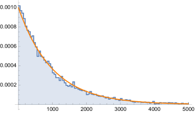
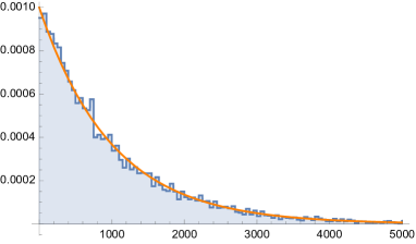
Figure 1. In orange, the PDF of an exponential distribution of mean $n$. In blue, the empirical PDF of the meeting time of two independent (left) and coupled (right) random walks starting from two states uniformly at random. The simulations are performed by sampling $10^{4}$ random DFAs with size $n=1000$. We used $r=2$ for the top row, and $r=20$ for the bottom one.

2.1.2. Synchronization of a DFA, Černỳ’s conjecture, and coalescence

Beyond learning theory, DFAs are known to be the object of a long-standing open problem due to Černỳ [10]. The so-called Černỳ’s conjecture is related to the notion of synchronization of a DFA. A given DFA is synchronizable if there exists a word $w$ such that $w(x)=w(y)$ for every $x,y\in V$; such a word is said to be a synchronizing word for the DFA. Clearly, if a DFA is synchronizable, then there exist arbitrarily many synchronizing words. The conjecture amounts to the claim that, if a DFA is synchronizable, then the length of the shortest synchronizing word is at most $(n-1)^{2}$. In that same work [10], the author constructs an example of a DFA having a word of length exactly $(n-1)^{2}$ as the shortest synchronizing word. Therefore, if the conjecture were true, then $(n-1)^{2}$ would be a sharp bound. Relaxing a bit the problem, one strategy is to look for a high-probability result which ensure the existence of short synchronizing words when the DFA is sampled at random. Along these lines, Nicaud [26, 27] recently showed that, when the DFA is taken uniformly at random, then there exists a synchronizing word of length $O(n\log^{3}(n))$ with high probability. More precisely, letting $\tau_{\rm sync}$ denote the smallest $t\in\mathbb{N}$ for which the random word $W_{t}$ is synchronizing, and using the notation introduced in 2.4:

Theorem 2.6 ([27]).

W.h.p., there exists a constant $c>0$ such that

(2.7) $$\mathbf{Q}\left(\tau_{\rm sync}\leq cn\log^{3}(n)\right)\geq r^{-cn\log^{3}(n)}\;\text{.}$$

Roughly speaking, this result implies that Černỳ’s conjecture holds for most large automata, and that the upper bound $(n-1)^{2}$ is far from being tight for a typical DFA. Nonetheless, Nicaud’s result does not provide an answer to the question “how rare are such short synchronizing words?”. More precisely, taking a random word $W_{t}$ of length $t>0$, and letting $p_{t}$ be the probability that $W_{t}$ is synchronizing for a quenched realization of the DFA, what is the behavior of the random sequence $(p_{t})_{t\geq 0}$ for large DFAs?

As for the meeting problem described in Section 2.1.1, this synchronization problem may be approximated by means of a system of coalescing random walks, which we now describe. Let $n$ walks start from all distinct vertices, let them evolve synchronously but independently (i.e., each following an independent word), and when two or more particles meet, they merge together and evolve as a single walk (i.e., they follow the same word only after their meeting). We let $\mathbf{{\color[rgb]{0,0,0}P}}_{\rm coal}$ denote the law of this Markov chain, and define the coalescing time $\tau_{\rm coal}$ as the first time in which only one of the $n$ walks is left. By Theorem 2.1 and a union bound, it is immediate to check that

(2.8) $$\mathbf{{\color[rgb]{0,0,0}P}}_{\rm coal}\left(\tau_{\rm coal}>\left(1+\varepsilon\right)n\log n\right)\overset{\mathbb{P}}{\longrightarrow}0\;\text{,}\;\;\qquad\varepsilon>0\;\text{.}$$

Actually, since the single random walk on a random DFA satisfies w.h.p. the mean field conditions in [29], Theorem 1.2 therein and Proposition 3.3 below (that is, essentially the claim in Theorem 2.2, but with the two walks starting independently from stationarity) prescribe the limit distribution of $\tau_{\rm coal}$: letting $Z_{2},Z_{3},\ldots,Z_{i},\ldots$ be jointly independent random variables such that $Z_{i}\sim{\rm Exp}(\binom{i}{2})$,

(2.9) $$d_{W}\left(\frac{\tau_{\rm coal}}{n},\sum_{i=2}^{\infty}Z_{i}\right)\overset{\mathbb{P}}{\longrightarrow}0\;\text{,}\;\;\qquad$$

where $d_{W}\left(\,\cdot\,,\,\cdot\,\right)$ denotes the usual $L^{1}$-Wasserstein distance. In particular, Eq. 2.9 implies

(2.10) $$\frac{\mathbf{E}_{\rm coal}\left[\tau_{\rm coal}\right]}{n}\overset{\mathbb{P}}{\longrightarrow}2\;\text{,}\;\;$$

which, by Markov inequality, yields the following strengthening of Eq. 2.8: for every $\varepsilon>0$, there exists $c=c_{\varepsilon}>0$ such that, w.h.p.,

(2.11) $$\mathbf{{\color[rgb]{0,0,0}P}}_{\rm coal}\left(\tau_{\rm coal}>cn\right)<\varepsilon\;\text{.}$$

Also in this case, simulations suggest that the two models (synchronization vs. coalescence) roughly share the same behavior (see Fig. 2). For this reason, it is natural to believe to the following:

Conjecture 2.7.

Using the notation introduced in 2.4,

(2.12) $$\frac{\mathbf{E}_{\mathbf{Q}}\left[\tau_{\rm sync}\right]}{n}\overset{\mathbb{P}}{\longrightarrow}2\;\text{.}$$

Therefore, for every $\varepsilon>0$, there exists $c=c_{\varepsilon}>0$ such that, w.h.p.,

(2.13) $$\mathbf{Q}\left(\tau_{\rm sync}>cn\right)\leq\varepsilon\;\text{.}$$

Notice that if the latter conjecture held, then it would also provide a sharpening of the results in [27], by proving that there exist synchronizing words of length $O(n)$, and actually most words of length $\omega(n)$ are synchronizing.

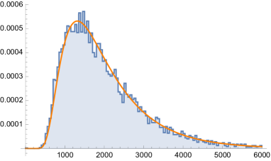
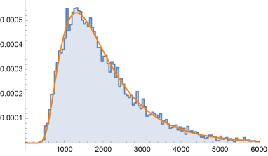
Figure 2. In orange, the PDF of the distribution of the random variable $n\sum_{i=2}^{\infty}Z_{i}$, where $Z_{i}$ is given as in Eq. 2.9. In blue, the empirical PDF of the coalescence time $\tau_{\rm coal}$ (left) and of the synchronization time $\tau_{\rm sync}$ (right). The simulations are performed by sampling $10^{4}$ random DFAs with size $n=1000$. We used $r=2$ for the first row and $r=20$ for the bottom one.

Remark 2.8.

In the context of random DFA, the condition in Eq. 2.1 that the $f$’s are one-to-one is often not required (see, e.g., [21, 27, 2]). (This condition translates into the constraint that a random DFA does not display multiple edges with the same origin-destination pair.) We impose this condition for the mere scope of importing without changes all the results in [7, 20], which are based on this assumption.

Nonetheless, it is immediate to check that, even when this constraint is neglected, the number of such multiple edges stays bounded with high probability. Given this, it should not be too hard to extend the results therein to the unconstrained setting. Nevertheless, this attempt is out of the scope of the present paper.

3. Auxiliary chain and First Visit Time Lemma

As in other related works (e.g., [15, 29]), our strategy of proof is based on interpreting the meeting time for two walks as the hitting time of the diagonal

(3.1) $$\Delta\coloneqq\{(x,x):x\in V\}$$

for the product chain $\mathbf{X}^{(2)}_{t}=(X^{(1)}_{t},X^{(2)}_{t})$. Clearly, such a hitting time is independent on transition probabilities from the diagonal, therefore in this analysis the product chain may be replaced by any other chain behaving as $\mathbf{X}^{(2)}_{t}$ until the first hitting of $\Delta$.

In what follows, we adopt this idea, introducing an effective auxiliary process (Section 3.1) for which the hypothesis of the First Visit Time Lemma (Theorem 3.1 in Section 3.2) are shown to hold (Proposition 3.2 in Section 3.3).

3.1. Auxiliary chain $\Xi_{t}$

Fix a realization of the random DFA $G$, and fix a stationary measure $\pi$ for the associated chain. In this setting, we introduce an auxiliary chain $(\Xi_{t})_{t\in\mathbb{N}}$ on the state space

(3.2) $$\tilde{V}\coloneqq V^{2}_{\not=}\sqcup\{\Delta\}\coloneqq\left\{(x,x^{\prime})\in V^{2}:x\neq x^{\prime}\right\}\sqcup\{\Delta\}\;\text{,}\;\;$$

namely the set $V^{2}$ in which elements in $\Delta$ are identified, and now $\Delta$ is considered as a state for this new chain. In words, such a Markov chain has the same behavior as that of two independent walks when the two walks are off the diagonal. When the two walks reach the diagonal $\Delta$, then they move independently out of the same vertex $z\in V$ sampled with probability proportional to $\pi(z)^{2}$. More precisely, the law of such a chain (given the underlying DFA $G$), which will be referred to as $(\tilde{\mathbf{{\color[rgb]{0,0,0}P}}}_{\xi})_{\xi\in\tilde{V}}$, is the one induced by the transition matrix $\tilde{P}$ given by (here, $(x,x^{\prime}),(y,y^{\prime})\in V^{2}_{\not=}$)

$$\tilde{P}(\xi,\zeta)\coloneqq\begin{cases}P(x,y)P(x^{\prime},y^{\prime})&\text{if}\ \xi=(x,x^{\prime})\;\text{,}\;\;\zeta=(y,y^{\prime})\\ \sum_{z\in V}P(x,z)P(x^{\prime},z)&\text{if}\ \xi=(x,x^{\prime})\;\text{,}\;\;\zeta=\Delta\\ \sum_{z\in V}\frac{\pi(z)^{2}}{\sum_{w\in V}\pi(w)^{2}}P(z,y)P(z,y^{\prime})&\text{if}\ \xi=\Delta\;\text{,}\;\;\zeta=(y,y^{\prime})\\ \frac{1}{r}&\text{if}\ \xi,\zeta\in\Delta\;\text{.}\end{cases}$$

As already observed in [25, §2.3], whenever the chain $P$ admits $\pi$ as its unique stationary measure, then

(3.3) $$\tilde{\pi}(\xi)\coloneqq\begin{cases}\pi(x)\pi(x^{\prime})&\text{if}\ \xi=(x,x^{\prime})\\ \sum_{z\in V}\pi(z)^{2}&\text{if}\ \xi=\Delta\;\text{.}\end{cases}$$

is the unique stationary measure for $\tilde{P}$.

3.2. First Visit Time Lemma

Given a growing sequence of Markov chains, the so-called First Visit Time Lemma (FVTL) [11] (see also [25]) is a powerful tool for the asymptotic analysis of hitting times when starting from stationarity. Originally motivated by the study of cover times of random walks on random graphs, Cooper and Frieze developed this criterion and successfully applied it to several problems (see, e.g., [11, 12, 13, 14]). More recently, the authors in [25] provided a new proof of such a lemma, linking this result to the theory of quasi-stationary distributions and metastability for Markov chains, in the spirit of previous works from the ’80, see, e.g., [1].

Before presenting a detailed version of the theorem, we briefly explain in words its content. To this purpose, consider a (discrete-time) ergodic Markov chain on a finite set $[N]$, with transition matrix $Q$, and with stationary measure $\mu$; further, consider the corresponding mixing times, i.e.,

(3.4) $$t_{\rm mix}=t_{\rm mix}(Q)\coloneqq\inf\left\{t\in\mathbb{N}\>\bigg{\rvert}\>\max_{z\in[N]}\left\|Q^{t}(z,\,\cdot\,)-\mu\right\|_{\rm TV}\leq\frac{1}{2e}\right\}\;\text{,}\;\;$$

where $\left\|\nu_{1}-\nu_{2}\right\|_{\rm TV}$ denotes the total-variation distance between two probability measures $\nu_{1}$ and $\nu_{2}$ defined on the same space. Roughly speaking, the FVTL asserts that for a growing (i.e., $N\to\infty$) sequence of Markov chains in which the mixing time is sufficiently small compared to the stationary measure of a target state, then the hitting times of such a target state is geometrically distributed when starting from stationarity.

Theorem 3.1 (FVTL).

Consider a sequence of ergodic Markov chains with state spaces $[N]$, transition matrices $Q=Q_{N}$, and unique stationary measures $\mu=\mu_{N}$. Further, consider a sequence of target states $\partial=\partial_{N}\in{\rm supp}(\mu)\subseteq[N]$ and assume that

(3.5) $$\mu(\partial)\,t_{\rm mix}\,\log\left(\frac{1}{\min_{z\in{\rm supp}(\mu)}\mu(z))}\right)\underset{N\to\infty}{\longrightarrow}0\;\text{.}$$

Then, there exists some $\lambda=\lambda_{N}\in(0,1)$ such that

(3.6) $$\sup_{t\geq 0}\left|\frac{\Pr(\tau_{\partial}>t\>|\>X_{0}\sim\mu)}{(1-\lambda)^{t}}-1\right|\underset{N\to\infty}{\longrightarrow}0\;\text{.}$$

Moreover, for any sequence $T=T_{N}$ satisfying

(3.7) $$T\geq 2t_{\rm mix}\,\log\left(\frac{1}{\min_{z\in{\rm supp}(\mu)}\mu(z)}\right)\qquad\text{and}\qquad\mu(\partial)\,T\underset{N\to\infty}{\longrightarrow}0\;\text{,}\;\;$$

we have

(3.8) $$\frac{\lambda}{\mu(\partial)/R}\underset{N\to\infty}{\longrightarrow}1\;\text{,}\;\;\qquad\text{with}\ R=R_{N,T}\coloneqq\sum_{t=0}^{T}Q^{t}(\partial,\partial)\;\text{.}$$

Henceforth, the FVTL not only asserts that the mixing condition in Eq. 3.5 guarantees the asymptotic geometric distribution of the hitting time of the target (cf. Eq. 3.6), but also identify the asymptotic behavior of the parameter of the geometric distribution (cf. Eq. 3.8). Indeed, as Eq. 3.8 shows, $\lambda$ is asymptotically prescribed by:

• $\mu(\partial)$, the stationary value of the target;

• $R$, the mean number of returns to the target within time $T$.

Finally, we remark that this version of the FVTL is a slightly more convenient rewriting of the one presented in [25, Theorem 2.2]. The main difference is that here we do not assume the sub-Markovian chain $[Q]_{\partial}$ (in which the row and column associated to the target state $\partial$ have been erased) to be irreducible. This condition is not crucial, as already pointed out, e.g., in [1, Remark 3.8]. For the sake of completeness, we report a complete and self-contained proof of Theorem 3.1 in Appendix A.

3.3. Auxiliary chain and FVTL

We now apply the FVTL to the auxiliary chain $\Xi_{t}$ introduced above. In this context, $N=n(n-1)+1$, $Q=\tilde{P}$, $\mu=\tilde{\pi}$, and $\partial=\Delta$. In particular, recall that $[\tilde{P}]_{\Delta}$ denotes the sub-Markovian transition matrix obtained by $\tilde{P}$ by removing the state $\Delta$. Therefore, in order to verify the assumptions of Theorem 3.1, it suffices to show the validity of the following lemma.

Proposition 3.2.

Let $G$ be a random DFA, and consider the process $\Xi_{t}$ defined in Section 3.1. Letting $T\coloneqq\lceil\log^{5}(n)\rceil$, $S\coloneqq\lceil\log^{3}(n)\rceil$, and $\varepsilon\in(0,1)$, we consider the following events:

(3.9) $$\mathcal{A}_{1} \coloneqq\left\{\min_{\xi\in{\rm supp}(\tilde{\pi})\subseteq\tilde{V}}\tilde{\pi}(\xi)\geq n^{-3.6}\right\}\;\text{,}\;\;$$

(3.10) $$\mathcal{A}_{2} \coloneqq\left\{\max_{\xi\in\tilde{V}}\tilde{\pi}(\xi)\leq\frac{\log^{8}(n)}{n}\right\}\;\text{,}\;\;$$

(3.11) $$\mathcal{A}_{3} \coloneqq\left\{\left|n\,\tilde{\pi}(\Delta)-\frac{r}{r-1}\right|<\varepsilon\right\}\;\text{,}\;\;$$

(3.12) $$\mathcal{A}_{4} {\color[rgb]{0,0,0}\coloneqq\left\{\max_{\xi\in\tilde{V}}\|\tilde{P}^{S}(\xi,\cdot)-\tilde{\pi}\|_{\rm TV}<\varepsilon\right\}}\;\text{,}\;\;$$

(3.13) $$\mathcal{A}_{5} \coloneqq\left\{\left|\left(\sum_{t=0}^{T}\tilde{P}^{t}(\Delta,\Delta)\right)-\frac{r}{r-1}\right|<\varepsilon\right\}\;\text{.}$$

Then, for every $\varepsilon>0$, $\cap_{i=1}^{5}\,\mathcal{A}_{i}$ occurs w.h.p..

Theorems 3.1 and 3.2, and the fact that $P\otimes P$ and $\tilde{P}$ coincide out of $\Delta$, immediately yield the following result:

Proposition 3.3.

Let $G$ be a random DFA and consider two independent walks on $G$. Then, there exists a sequence of random variables $\Lambda=\Lambda_{n}\in(0,1)$ such that

(3.14) $$n\,\Lambda\overset{\mathbb{P}}{\longrightarrow}1\;\text{,}\;\;\qquad\sup_{t\geq 0}\left|\frac{\mathbf{{\color[rgb]{0,0,0}P}}_{\pi\otimes\pi}(\tau_{\rm meet}>t)}{(1-\Lambda)^{t}}-1\right|\overset{\mathbb{P}}{\longrightarrow}0\;\text{.}$$

Section 4 is devoted to the proof of Proposition 3.2. In Section 5 we use Proposition 3.3 to deduce Theorems 2.1 and 2.2.

Remark 3.4.

As already pointed out in right below Corollary 2.3, the asymptotic distribution of the meeting time does not depend on $r$, the out-degree. Indeed, while the intuition that it should depend on $r$ seems plausible, actually — as the First Visit Time Lemma rigorously prescribes — the mean of the meeting time asymptotically depends on the ratio between the following two quantities: the stationary measure of the diagonal over the expected sojourn time on the diagonal (within the mixing time). Since both such quantities are asymptotically equal (up to normalization) to $r/(r-1)$ (see Eqs. 3.11 and 3.13), the dependence on $r$ cancels out, w.h.p., in the asymptotic distribution of the meeting time.

4. Meeting time starting from stationarity. Proof of Proposition 3.2

Throughout the rest of the paper, for notational convenience, we omit writing the integer part $\lceil\,\cdot\,\rceil$ of all time variables.

In order to prove Proposition 3.2, we start by recalling some known results on the behavior of a single random walk and its stationary measure on the random DFA $G$.

Theorem 4.1 ([7, 2, 20]).

Let $G$ be a random DFA.

• Uniqueness of the stationary measure ([7, Theorem 1]): w.h.p.,

  (4.1) $$\exists!\,\pi:\pi P=\pi\;\text{.}$$

• Mixing with cutoff ([7, Theorem 1]): for $\alpha>0$ and $t_{\alpha}\coloneqq\alpha\log(n)$, w.h.p.,

  (4.2) $$\max_{x\in V}\left|\|P^{t_{\alpha}}(x,\cdot)-\pi\|_{\rm TV}-\mathds{1}_{\left(-\infty,\frac{1}{\log(r)}\right)}(\alpha)\right|\overset{\mathbb{P}}{\longrightarrow}0\;\text{,}\;\;\qquad\alpha\neq\frac{1}{\log(r)}\;\text{.}$$

• Minimum of $\pi$ ([2, Theorem 35]): w.h.p.,

  (4.3) $$\min_{x\in{\rm supp}(\pi)}\pi(x)\geq\frac{1}{n^{1.8}}\;\text{.}$$

• Maximum of $\pi$ ([20, Lemma 4.2]): w.h.p.,

  (4.4) $$\max_{x\in V}\pi(x)\leq\frac{\log^{8}(n)}{n}\;\text{.}$$

In this rest of this section, we focus on the auxiliary chain $\Xi_{t}$ introduced in Section 3. Let us observe that, since Eq. 4.1 occurs w.h.p., when proving Proposition 3.2, we will implicitly assume that the random DFA $G$ gives rise to an ergodic chain $(P,\pi)$; by the discussion at the end of Section 3.1, the auxiliary chain $\Xi_{t}$ has a unique stationary measure $\tilde{\pi}$ as given in Eq. 3.3.

4.1. Organization of the proof of Proposition 3.2

The rest of the section is divided into three parts.

In Section 4.2, we control the probability of the events $\mathcal{A}_{1}$, $\mathcal{A}_{2}$ and $\mathcal{A}_{3}$, i.e., we bound extremal entries of $\tilde{\pi}$ and provide the first order asymptotics of $\tilde{\pi}(\Delta)$. While the former control easily follows from Theorem 4.1 and is the content of Lemmas 4.2 and 4.3, the latter requires a deeper analysis, which we carry out in Lemma 4.4.

In Section 4.3, we analyze the mixing time of the auxiliary chain, showing in Proposition 4.5 that, w.h.p., $\mathcal{A}_{4}$ holds. The proof of this result relies on the mixing result in Theorem 4.1 for a single walk and on a coupling of the the auxiliary chain with two independent walks. This part is divided into three main lemmas, Lemmas 4.7, 4.6 and 4.8, which essentially show that, once the auxiliary chain exits the state $\Delta$, it can be coupled with the product chain for a polylogarithmic number of steps at a small TV-cost.

Finally, exploiting the tools developed in Section 4.3, in Section 4.4 we focus on the number of returns to $\Delta$ for the auxiliary chain, ensuring that, w.h.p., $\mathcal{A}_{5}$ holds.

4.2. Estimating $\tilde{\pi}$

Recall the events $\mathcal{A}_{1}$, $\mathcal{A}_{2}$ and $\mathcal{A}_{3}$ in Eqs. 3.9, 3.11 and 3.10. In the following three lemmas, we respectively show that $\lim_{n\to\infty}\mathbb{P}(\mathcal{A}_{i})=1$ for $i=1,2,3$.

Lemma 4.2 (Minimum of $\tilde{\pi}$).

$\lim_{n\to\infty}\mathbb{P}(\mathcal{A}_{1})=1$.

Proof.

By Cauchy-Schwarz inequality, $\tilde{\pi}(\Delta)\geq n^{-1}$, while Eqs. 3.3 and 4.3 yield

$$\min_{\xi\neq\Delta}\tilde{\pi}(\xi)\geq\frac{1}{n^{3.6}}\;\text{.}$$

This concludes the proof of the lemma. ∎

Lemma 4.3 (Maximum of $\tilde{\pi}$).

$\lim_{n\to\infty}\mathbb{P}(\mathcal{A}_{2})=1$.

Proof.

By the definition of $\tilde{\pi}$ in Eq. 3.3, Hölder inequality yields

$$\max_{\xi\in\tilde{V}}\tilde{\pi}(\xi)\leq\max\left\{\max_{(x,y)\in V^{2}_{\not=}}\pi(x)\pi(y)\;\text{,}\;\;\tilde{\pi}(\Delta)\right\}\leq\max_{x\in V}\pi(x)\;\text{.}$$

Eq. 4.4 concludes the proof of the lemma. ∎

Lemma 4.4 (Value of $\tilde{\pi}(\Delta)$).

$\lim_{n\to\infty}\mathbb{P}(\mathcal{A}_{3})=1$, for every $\varepsilon>0$.

Proof.

Recall the definition of $\tilde{\pi}$ from Eq. 3.3, and fix $t\coloneqq\log^{3}(n)$. Instead of proving the desired claim directly, we first show that, letting

(4.5) $$Y\coloneqq\frac{1}{n^{2}}\sum_{y,z\in V}\sum_{x\in V}P^{t}(y,x)P^{t}(z,x)\;\text{,}\;\;$$

the following two claims hold:

(4.6) $$\mathbb{E}\left[Y\right]=\frac{1}{n}\frac{r}{r-1}+o\left(\frac{1}{n}\right)\;\text{,}\;\;$$

and

(4.7) $$\mathbb{E}[Y^{2}]\leq\mathbb{E}\left[Y\right]^{2}+o\left(\frac{1}{n^{2}}\right)\;\text{.}$$

Eqs. 4.6 and 4.7 conclude the proof of the lemma. Indeed, by the triangle and Chebyshev inequalities,

$$\mathbb{P}\left(\left|n\tilde{\pi}(\Delta)-\frac{r}{r-1}\right|>\varepsilon\right)$$

$$\qquad\leq\mathbb{P}\left(\left|n\tilde{\pi}(\Delta)-nY\right|>\frac{\varepsilon}{2}\right)+n^{2}\frac{\mathbb{E}[Y^{2}]-\mathbb{E}\left[Y\right]^{2}}{(\varepsilon/4)^{2}}+\mathds{1}_{(\frac{\varepsilon}{4},\infty)}\left(\left|n\mathbb{E}\left[Y\right]-\frac{r}{r-1}\right|\right)\;\text{.}$$

While the second and third terms on the right-hand side above vanish as $n\to\infty$ by Eqs. 4.6 and 4.7, the first term vanishes by the fact that $t$ is order $\log^{2}(n)$ times the mixing time (see Eq. 4.2):

$$\lim_{n\to\infty}\mathbb{P}\left(\max_{x,y\in V}\left|P^{t}(x,y)-\pi(y)\right|\leq n^{-2}\right)=1\;\text{.}$$

We are left to show the validity of Eqs. 4.6 and 4.7. As a general strategy, we employ a system of four annealed random walks (see [7, Section 2.2]) running for a time $t=\log^{3}(n)$. Roughly speaking, starting from an empty environment, we construct the whole trajectories of these walks one at the time, and concurrently construct the environment that these walks explore. More precisely, let

$$\left(\left(Z^{(1)}_{s},Z^{(2)}_{s},Z^{(3)}_{s},Z^{(4)}_{s}\right)\right)_{s=0}^{t}\in(V^{4})^{t+1}\;\text{,}\;\;$$

be the non-Markovian process with law $\mathbb{P}^{\rm an}$ constructed as follows:

1. Initially, set the environment, say $\sigma^{(1)}$, to consist of an “empty graph”, i.e., $\sigma^{(1)}_{0}\coloneqq\varnothing$.

2. Select a uniformly random vertex $y\in V$, and consider a walk $Z^{(1)}$ starting at $y$, i.e., $Z^{(1)}_{0}\coloneqq y$.

3. At every step $s\in\{0,\ldots,t\}$, given the current environment $\sigma^{(1)}_{s}$ and position of the walk $Z^{(1)}_{s}$, the walk picks a uniformly random color $c\in\mathcal{C}$ and looks at the associated out-going edge from $Z^{(1)}_{s}$:

   • If the $c$-tail of the vertex $Z^{(1)}_{s}$ is unmatched, select a uniformly random destination among all vertices in $V$ which have no directed edge from $Z^{(1)}_{s}$, yet. Then, call $\sigma^{(1)}_{s+1}$ the new environment obtained from $\sigma^{(1)}_{s}$ by adding this new edge, and move the walk to this vertex.

   • If the $c$-tail of the vertex $Z^{(1)}_{s}$ is already matched, i.e., the $c$-colored directed out-going edge from $Z^{(1)}_{s}$ already belongs to the environment $\sigma^{(1)}_{s}$, then simply set $\sigma^{(1)}_{s+1}\coloneqq\sigma^{(1)}_{s}$, and move the walk to the end-point of the $c$-tail attached to $Z^{(1)}_{s}$.

4. Once the first walk $Z^{(1)}$ has completed its trajectory of length $t$, perform the same procedure for the second walk $Z^{(2)}$, but this time starting with the environment $\sigma^{(2)}_{0}\coloneqq\sigma^{(1)}_{t}$, i.e., the environment already revealed by the trajectory of $Z^{(1)}$. Similarly for $Z^{(3)}$ and $Z^{(4)}$, respectively with starting environments $\sigma^{(3)}_{0}\coloneqq\sigma^{(2)}_{t}$ and $\sigma^{(4)}_{0}\coloneqq\sigma^{(3)}_{t}$.

These annealed walks provide us with an alternative expression for $\mathbb{E}[Y]$ and $\mathbb{E}[Y^{2}]$: recalling $Y$ in Eq. 4.5,

(4.8) $$\mathbb{E}[Y]=\mathbb{P}^{\rm an}\big{(}Z^{(1)}_{t}=Z^{(2)}_{t}\big{)}\;\text{,}\;\;$$

and

(4.9) $$\mathbb{E}[Y^{2}]=\mathbb{P}^{\rm an}\big{(}Z^{(1)}_{t}=Z^{(2)}_{t}\;\text{,}\;\;Z^{(3)}_{t}=Z^{(4)}_{t}\big{)}\;\text{.}$$

We start with the proof of Eq. 4.6 using Eq. 4.8. To this purpose, letting

(4.10) $$\mathcal{N}\coloneqq\bigsqcup_{x\in V}\mathcal{N}_{x}\coloneqq\bigsqcup_{x\in V}\{Z^{(1)}_{t}=Z^{(2)}_{t}=x\}\;\text{,}\;\;$$

we have

(4.11) $$\mathbb{P}^{\rm an}\big{(}Z^{(1)}_{t}=Z^{(2)}_{t}\big{)}=\sum_{x\in V}\mathbb{P}^{\rm an}(\mathcal{N}_{x})\;\text{,}\;\;$$

and, by symmetry, all the summands in the last display are equal. Therefore, fix any arrival point $x\in V$ for the two walks, and define the events

$$\mathcal{N}^{(i)}_{x}\coloneqq\{Z^{(i)}_{t}=x\}\;\text{,}\;\;\qquad i=1,2\;\text{.}$$

We now show

(4.12) $$\mathbb{P}^{\rm an}\big{(}\mathcal{N}_{x}\big{)}=\left(1+o(1)\right)\frac{1}{n^{2}}\frac{r}{r-1}\;\text{,}\;\;$$

from which Eq. 4.6 follows (combine Eq. 4.12 with Eqs. 4.8 and 4.11). The proof of Eq. 4.12 goes through the following steps:

• Consider the event for $Z^{(1)}$ of arriving at $x\in V$ performing a loop, i.e.,

  $$\mathcal{N}^{(1),{\rm bad}}_{x}\coloneqq\mathcal{N}^{(1)}_{x}\cap\mathcal{L}^{(1)}\coloneqq\mathcal{N}^{(1)}_{x}\cap\{Z^{(1)}_{s}=Z^{(1)}_{s^{\prime}}\ \text{for some}\ s<s^{\prime}\leq t\}\;\text{,}\;\;$$

  and let

  $$\mathcal{N}_{x}^{(1),{\rm good}}\coloneqq\mathcal{N}^{(1)}_{x}\setminus\mathcal{N}^{(1),{\rm bad}}_{x}$$

  denote the event that $x$ was hit at time $t$ without loops. In order to estimate $\mathbb{P}^{\rm an}\big{(}\mathcal{N}_{x}^{(1),{\rm bad}}\big{)}$, we further distinguish the case in which $x$ was ever hit before time $t$; thus, letting $[Z^{(1)}]\coloneqq\{Z_{0}^{(1)},\ldots,Z_{t-1}^{(1)}\}$ and $\mathcal{H}^{(1)}_{x}\coloneqq\{x\in[Z^{(1)}]\}$,

  (4.13) $$\begin{aligned} \mathbb{P}^{\rm an}\big{(}\mathcal{N}^{(1),{\rm bad}}_{x}\big{)}&\leq\mathbb{P}^{\rm an}\big{(}\mathcal{N}^{(1)}_{x}\mid(\mathcal{H}^{(1)}_{x})^{c}\cap\mathcal{L}^{(1)}\big{)}\mathbb{P}^{\rm an}\big{(}\mathcal{L}^{(1)}\big{)}+\mathbb{P}^{\rm an}\big{(}\mathcal{N}^{(1)}_{x}\cap\mathcal{H}^{(1)}_{x}\big{)}\\ &\qquad\leq\frac{1}{n}\times\frac{t^{2}}{n}+\frac{t^{3}}{n^{2}}\leq\frac{2t^{3}}{n^{2}}\;\text{.}\end{aligned}$$

  Indeed, $\mathbb{P}^{\rm an}\big{(}\mathcal{N}^{(1)}_{x}\mid(\mathcal{H}^{(1)}_{x})^{c}\cap\mathcal{L}^{(1)}\big{)}\leq\frac{1}{n}$ holds because the event requires to connect to vertex $x$ at time $t$; $\mathbb{P}^{\rm an}\left(\mathcal{L}^{(1)}\right)\leq\frac{t^{2}}{n}$ comes from estimating by a union bound the probability of the event that, within $t$ steps, the walk ever hits one of the previously visited vertices, which are at most $t$. Finally, $\mathbb{P}^{\rm an}\left(\mathcal{N}_{x}^{(1)}\cap\mathcal{H}_{x}^{(1)}\right)$ is estimated by the probability that the walk visits $x$ for the first time within time $t-1$ (this occurs with probability less than $\frac{t}{n}$), and then visits one of the vertices which have been previously visited (this happens with probability less than $\frac{t^{2}}{n}$).

• By an analogous argument and Eq. 4.13, we obtain

  (4.14) $$\mathbb{P}^{\rm an}\big{(}\mathcal{N}_{x}^{(1),\rm bad}\cap\mathcal{N}_{x}^{(2)}\big{)}\leq\mathbb{P}^{\rm an}\left(\mathcal{N}_{x}^{(1),\rm bad}\right)\times\frac{t^{2}}{n}\leq\frac{2t^{5}}{n^{3}}\;\text{.}$$

• We now estimate $\mathbb{P}^{\rm an}\big{(}\mathcal{N}^{(1),{\rm good}}_{x}\cap\mathcal{N}^{(2)}_{x}\big{)}$. Under $\mathcal{N}_{x}^{(1),{\rm good}}$, the second walk $Z^{(2)}$ can reach the same $x\in V$ at time $t$ in either one of the following two ways:

  • $Z^{(2)}$ hits the trajectory of the first walk for the first time at time $s\leq t$ in the unique vertex that is at distance $t-s$ from $x$, and then follows the same path: letting $\{Z^{(1)}\}\coloneqq\{Z^{(1)}_{0},\ldots,Z^{(1)}_{t}\}$,

    $$\mathcal{N}^{(2),{\rm good}}_{x}\coloneqq\bigsqcup_{s=0}^{t}\{Z^{(2)}_{s^{\prime}}\notin\{Z^{(1)}\}\ \text{for all}\ 0\leq s^{\prime}<s\}\cap\{Z^{(1)}_{s^{\prime}}=Z^{(2)}_{s^{\prime}}\ \text{for all}\ s\leq s^{\prime}\leq t\}\;\text{.}$$

    Then, since $t=\log^{3}(n)$,

    (4.15) $$\begin{aligned} \mathbb{P}^{\rm an}\big{(}\mathcal{N}^{(1),{\rm good}}_{x}\cap\mathcal{N}^{(2),{\rm good}}_{x}\big{)}&=\mathbb{P}^{\rm an}\big{(}\mathcal{N}^{(2),{\rm good}}_{x}\mid\mathcal{N}^{(1),{\rm good}}_{x}\big{)}\left(1+o(1)\right)\frac{1}{n}\\ &=\left(\sum_{s=0}^{t}\left(1+O\left(\frac{t}{n}\right)\right)^{s}\frac{1}{n}\left(\frac{1}{r}\right)^{t-s}\right)\left(1+o(1)\right)\frac{1}{n}\\ &=\frac{1}{n^{2}}\left(\frac{r}{r-1}+o(1)\right)\;\text{.}\end{aligned}$$

    where the first asymptotic equality follows from the definition of $\mathcal{N}^{(1),{\rm good}}_{x}$ and Eq. 4.13.

  • $Z^{(2)}$ hits at some time the path of the first walk, exits at least once the path, and eventually re-enters that same path: recalling $\{Z^{(1)}\}\coloneqq\{Z^{(1)}_{0},\ldots,Z^{(1)}_{t}\}$,

    $$\mathcal{N}^{(2),{\rm bad}}_{x}\coloneqq\{Z_{s_{1}}^{(2)},Z_{s_{3}}^{(2)}\in\{Z^{(1)}\}\;\text{,}\;\;Z_{s_{2}}^{(2)}\notin\{Z^{(1)}\}\;\text{,}\;\;\text{for some}\ 0\leq s_{1}<s_{2}<s_{3}\leq t\}\;\text{.}$$

    Note that $\mathcal{N}^{(2),{\rm bad}}_{x}\neq\big{(}\mathcal{N}^{(2)}_{x}\setminus\mathcal{N}^{(2),{\rm good}}_{x}\big{)}$, but

    $$\mathcal{N}^{(1),{\rm good}}_{x}\cap\big{(}\mathcal{N}_{x}^{(2)}\setminus\mathcal{N}^{(2),{\rm good}}_{x}\big{)}\subset\mathcal{N}^{(1),{\rm good}}_{x}\cap\mathcal{N}^{(2),{\rm bad}}_{x}\;\text{.}$$

    Hence, we obtain

    (4.16) $$\mathbb{P}^{\rm an}\big{(}\mathcal{N}^{(1),{\rm good}}_{x}\cap\big{(}\mathcal{N}_{x}^{(2)}\setminus\mathcal{N}^{(2),{\rm good}}_{x}\big{)}\big{)} \leq\mathbb{P}^{\rm an}(\mathcal{N}^{(1),{\rm good}}_{x}\cap\mathcal{N}^{(2),{\rm bad}}_{x})$$

    $$\leq(1+o(1))\frac{1}{n}\times\frac{t^{2}}{n}\times\frac{2t^{2}}{n}=o\left(\frac{1}{n^{2}}\right)\;\text{.}$$

• In conclusion, since

  $$\mathbb{P}^{\rm an}\big{(}\mathcal{N}_{x}^{(1),{\rm good}}\cap\mathcal{N}_{x}^{(2),{\rm good}}\big{)}\leq\mathbb{P}^{\rm an}\big{(}\mathcal{N}_{x}\big{)} \leq\mathbb{P}^{\rm an}\big{(}\mathcal{N}_{x}^{(1),{\rm good}}\cap\mathcal{N}_{x}^{(2),{\rm good}}\big{)}$$

  $$\qquad+\mathbb{P}^{\rm an}\big{(}\mathcal{N}_{x}^{(1),{\rm bad}}\cap\mathcal{N}_{x}^{(2)}\big{)}$$

  $$\qquad+\mathbb{P}^{\rm an}\big{(}\mathcal{N}_{x}^{(1),{\rm good}}\cap\mathcal{N}_{x}^{(2),{\rm bad}}\big{)}\;\text{,}\;\;$$

  the estimates in Eqs. 4.14, 4.15 and 4.16 show the validity of Eq. 4.12.

This concludes the proof of Eq. 4.6; we now prove Eq. 4.7 using Eq. 4.9. In analogy with Eq. 4.10, define

$$\mathcal{M}\coloneqq\bigsqcup_{y\in V}\mathcal{M}_{y}\coloneqq\bigsqcup_{y\in V}\{Z^{(3)}_{t}=Z^{(4)}_{t}=y\}\;\text{,}\;\;$$

and note that, by symmetry,

(4.17) $$\mathbb{P}^{\rm an}\big{(}\mathcal{M}\big{)}=\mathbb{P}^{\rm an}\big{(}\mathcal{N}\big{)}=\sum_{x\in V}\mathbb{P}^{\rm an}\left(\mathcal{N}_{x}\right)=\mathbb{E}\left[Y\right]\;\text{.}$$

Define further the following events:

$$\mathcal{M}^{\rm bad}\coloneqq\mathcal{M}\cap\{Z^{(i)}_{s}=Z^{(j)}_{s^{\prime}}\ \text{for some}\ i\in\{1,2\},j\in\{3,4\},s,s^{\prime}\in\{0,\dots,t\}\}\;\text{,}\;\;$$

and $\mathcal{M}^{\rm good}\coloneqq\mathcal{M}\setminus\mathcal{M}^{\rm bad}$. Then,

(4.18) $$\mathbb{E}[Y^{2}] =\sum_{x\in V}\mathbb{P}^{\rm an}\big{(}\mathcal{N}_{x}\cap\mathcal{M}\big{)}=\sum_{x\in V}\mathbb{P}^{\rm an}\big{(}\mathcal{N}_{x}\cap\mathcal{M}^{\rm good}\big{)}+\sum_{x\in V}\mathbb{P}^{\rm an}\big{(}\mathcal{N}_{x}\cap\mathcal{M}^{\rm bad}\big{)}\;\text{.}$$

As for the second sum above, we have

(4.19) $$\sum_{x\in V}\mathbb{P}^{\rm an}\big{(}\mathcal{N}_{x}\cap\mathcal{M}^{\rm bad}\big{)}\leq n\times\frac{3}{n^{2}}\times\left(\frac{2t^{2}}{n}\times\frac{3t^{2}}{n}+\frac{2t^{2}}{n}\times\frac{t^{2}}{n}\right)=o\left(\frac{1}{n^{2.5}}\right)\;\text{.}$$

where the factor $n$ comes from the sum and the symmetry of the model, the term $3/n^{2}$ follows from Eq. 4.12, and the term within brackets is an estimate of $\mathbb{P}^{\rm an}\big{(}\mathcal{M}^{\rm bad}\mid\mathcal{N}_{x}\big{)}$. For the latter we argue as follows: either the walk $Z^{(3)}$ hits one of the trajectories of $Z^{(1)}$ or $Z^{(2)}$ and, subsequently the walk $Z^{(4)}$ ends at the same point as $Z^{(3)}$; or the walk $Z^{(3)}$ does not hit $Z^{(1)}\cup Z^{(2)}$ and, subsequently, the walk $Z^{(4)}$ hits both $Z^{(1)}\cup Z^{(2)}$ and $Z^{(3)}$ (which at this point will be disjoint from $Z^{(1)}\cup Z^{(2)}$). For what concerns the first sum, we argue as follows: call $\sigma\in\mathcal{N}_{x}$ a realization of the paths of $Z^{(1)}$ and $Z^{(2)}$ realizing $\mathcal{N}_{x}$. For such a $\sigma$, call $\mathcal{M}^{\rm good}(\sigma)$ the set of paths of $Z^{(3)}$ and $Z^{(4)}$ realizing $\mathcal{M}$ and not intersecting $\sigma$. Then,

$$\mathbb{P}^{\rm an}\big{(}\mathcal{N}_{x}\cap\mathcal{M}^{\rm good}\big{)} =\sum_{\sigma\in\mathcal{N}_{x}}\sum_{\eta\in\mathcal{M}^{\rm good}(\sigma)}\mathbb{P}^{\rm an}(\sigma)\mathbb{P}^{\rm an}(\eta\mid\sigma)$$

$$=\sum_{\sigma\in\mathcal{N}_{x}}\sum_{\eta\in\mathcal{M}^{\rm good}(\sigma)}\mathbb{P}^{\rm an}(\sigma)\mathbb{P}^{\rm an}(\eta)$$

$$\leq\mathbb{P}^{\rm an}(\mathcal{N}_{x})\mathbb{P}^{\rm an}(\mathcal{M})\;\text{.}$$

By combining this with Eqs. 4.18, 4.19 and 4.17, we get

(4.20) $$\mathbb{E}[Y^{2}]\leq\mathbb{E}[Y]^{2}+o(n^{-2.5})\;\text{,}\;\;$$

and, thus, Eq. 4.7. This concludes the proof of the lemma. ∎

4.3. Mixing of auxiliary chain

This section is devoted to the proof of the fact that the auxiliary chain mixes, w.h.p., within time $S=\log^{3}(n)$. More precisely, recalling the event $\mathcal{A}_{4}$ in Eq. 3.12, we show:

Proposition 4.5.

$\lim_{n\to\infty}\mathbb{P}(\mathcal{A}_{4})=1$.

Recall that the auxiliary and the product chain can be perfectly coupled as long as the two walks do not sit on the same vertex. Nevertheless, despite the fact that the analogue of Proposition 4.5 for the product chain is an immediate corollary of Eq. 4.2, establishing this for the auxiliary chain requires a finer analysis on the visits to the diagonal.

We divide the proof of Proposition 4.5 into several intermediate steps (Lemmas 4.6, 4.7 and 4.8), and present the concluding arguments at the end of this section.

As a first step we show that, conditionally on having a DFA in which $x$ and $x^{\prime}$ have a common in-neighbor, the probability that the random DFA has the property that two independent walks starting at $(x,x^{\prime})$ meet in a short time is small.

Lemma 4.6.

For every sequence $(x,x^{\prime})=(x_{n},x_{n}^{\prime})\in V^{2}_{\not=}$, let

(4.21) $$\mathcal{E}_{x,x^{\prime}}\coloneqq\{x\text{ and }x^{\prime}\text{ have (at least) a common in-neighbor in $G$}\}\;\text{.}$$

Then, for every $t=t_{n}\geq 1$ and $\epsilon=\epsilon_{n}>0$,

(4.22) $$\mathbb{P}\big{(}\mathbf{{\color[rgb]{0,0,0}P}}_{(x,x^{\prime})}\big{(}\tau_{\rm meet}<t\big{)}>\epsilon\mid\mathcal{E}_{x,x^{\prime}}\big{)}\leq\frac{8}{\epsilon}\>\frac{\log^{2}(n)\>t^{2}}{n}\;\text{.}$$

Proof.

Note that $\mathbb{P}\big{(}\,\cdot\,\mid\mathcal{E}_{x,x^{\prime}}\big{)}$ can be sampled as follows:

1. To each vertex $y\in V$ attach two Bernoulli random variables, $W_{x}^{y}$ and $W_{x^{\prime}}^{y}$, having the following joint law:

   $$\Pr\left(W_{x}^{y}=0,W_{x^{\prime}}^{y}=0\right) =\frac{\binom{n-2}{r}}{\binom{n}{r}}$$

   (4.23) $$\Pr\left(W_{x}^{y}=1,W_{x^{\prime}}^{y}=1\right) =\frac{\binom{n-2}{r-2}}{\binom{n}{r}}$$

   $$\Pr\left(W_{x}^{y}=1,W_{x^{\prime}}^{y}=0\right) =\Pr\left(W_{x}^{y}=0,W_{x^{\prime}}^{y}=1\right)=\frac{\binom{n-2}{r-1}}{\binom{n}{r}}\;\text{.}$$

   (Here, “$W^{y}_{x}=1$” corresponds to constructing the directed edge $y\to x$ endowed with a random color.)

2. If $W_{x}^{y}+W_{x^{\prime}}^{y}\neq 2$ for all $y\in V$, then resample all variables $W$’s, restarting from Item 1.

3. For $y\in V$, if $W_{x}^{y}=1$, then connect $y\to x$ and assign this edge a random color, and similarly for $W_{x^{\prime}}^{y}$; if $W^{y}_{x}+W^{y}_{x^{\prime}}=2$, color the corresponding two edges with two distinct random colors.

4. Call $\sigma$ the partial environment generated so far (Items 1, 2 and 3).

5. Complete the rest of the random DFA: construct a colored digraph $G^{\prime}$ with the $n-2$ vertices in $V\setminus\{x,x^{\prime}\}$, and out-degrees $d_{y}^{+}=r-W_{x}^{y}-W_{x^{\prime}}^{y}$ for all $y\in V\setminus\{x,x^{\prime}\}$.

6. Call $G=G^{\prime}\cup\sigma$ the resulting DFA.

Let $\mathcal{F}_{x,x^{\prime}}$ be the event that $\sigma_{0}=\sigma$ constructed in Items 1, 2, 3 and 4 has no arrows outgoing $x$ nor $x^{\prime}$. We now show that there exists $C^{\prime}=C^{\prime}(r)>0$ such that

(4.24) $$\mathbb{P}\left(\mathcal{F}_{x,x^{\prime}}^{c}\mid\mathcal{E}_{x,x^{\prime}}\right)\leq\frac{C^{\prime}}{n}\;\text{.}$$

The proof of Eq. 4.24 goes as follows. Let $\{y\not\to z\}$ denote the event that no arrow from $y$ points to $z\in V$; then,

$$\mathbb{P}\left(\{x\not\to x\}\cap\{x\not\to x^{\prime}\}\right)=\left(1-\frac{2}{n}\right)\left(1-\frac{2}{n-1}\right)\cdots\left(1-\frac{2}{n-r+1}\right)\geq 1-\frac{3r}{n}\;\text{,}\;\;$$

where the last estimate holds for all $n$ sufficiently large. Therefore, by independence,

(4.25) $$\mathbb{P}\left(\mathcal{F}_{x,x^{\prime}}\right)\geq\left(1-\frac{3r}{n}\right)^{2}\geq 1-\frac{6r}{n}\;\text{.}$$

Recall further that

(4.26) $$\mathbb{P}\left(\mathcal{E}_{x,x^{\prime}}^{c}\right)=\mathbb{P}\left(\bigcap_{y\in[n]}\left\{\{y\not\to x\}\cup\{y\not\to x^{\prime}\}\right\}\right)=\left(1-\frac{\binom{n-2}{r-2}}{\binom{n}{r}}\right)^{n}=1-\Theta(n^{-1})\;\text{.}$$

By the bound in Eq. 4.26, we estimate the right-hand side in Eq. 4.24 as follows:

(4.27) $$\mathbb{P}\left(\mathcal{F}_{x,x^{\prime}}^{c}\mid\mathcal{E}_{x,x^{\prime}}\right)=\frac{\mathbb{P}\left(\mathcal{F}_{x,x^{\prime}}^{c}\cap\mathcal{E}_{x,x^{\prime}}\right)}{\mathbb{P}(\mathcal{E}_{x,x^{\prime}})}\leq O\left(n\right)\times\mathbb{P}\left(\mathcal{F}_{x,x^{\prime}}^{c}\cap\mathcal{E}_{x,x^{\prime}}\right)\;\text{.}$$

As a consequence, Eq. 4.24 holds if we show

(4.28) $$\mathbb{P}\left(\mathcal{F}_{x,x^{\prime}}^{c}\cap\mathcal{E}_{x,x^{\prime}}\right)=O(n^{-2})\;\text{.}$$

To the purpose of proving Eq. 4.28, introduce the event

(4.29) $$\mathcal{G}_{x,x^{\prime}}=\left(\{x\to x\}\cap\{x\to x^{\prime}\}\right)\cup\left(\{x^{\prime}\to x\}\cap\{x^{\prime}\to x^{\prime}\}\right)\;\text{,}\;\;$$

and write

(4.30) $$\mathbb{P}\left(\mathcal{F}_{x,x^{\prime}}^{c}\cap\mathcal{E}_{x,x^{\prime}}\right)=\mathbb{P}\left(\mathcal{F}_{x,x^{\prime}}^{c}\cap\mathcal{E}_{x,x^{\prime}}\cap\mathcal{G}_{x,x^{\prime}}\right)+\mathbb{P}\left(\mathcal{F}_{x,x^{\prime}}^{c}\cap\mathcal{E}_{x,x^{\prime}}\cap\mathcal{G}_{x,x^{\prime}}^{c}\right)\;\text{.}$$

We now bound the two probabilities on the right-hand side above. On the one hand,

(4.31) $$\mathbb{P}\left(\mathcal{F}_{x,x^{\prime}}^{c}\cap\mathcal{E}_{x,x^{\prime}}\cap\mathcal{G}_{x,x^{\prime}}\right)=\mathbb{P}\left(\mathcal{E}_{x,x^{\prime}}\cap\mathcal{G}_{x,x^{\prime}}\right)\leq\mathbb{P}\left(\mathcal{G}_{x,x^{\prime}}\right)\leq 2\frac{\binom{n-2}{r-2}}{\binom{n}{r}}=O(n^{-2})\;\text{,}\;\;$$

while, on the other hand,

(4.32) $$\mathbb{P}\left(\mathcal{F}_{x,x^{\prime}}^{c}\cap\mathcal{E}_{x,x^{\prime}}\cap\mathcal{G}_{x,x^{\prime}}^{c}\right)\leq\mathbb{P}\left(\mathcal{F}_{x,x^{\prime}}^{c}\right)\mathbb{P}\left(\mathcal{E}_{x,x^{\prime}}\mid\mathcal{G}_{x,x^{\prime}}^{c}\right)\leq\frac{6r}{n}(n-2)\frac{\binom{n-2}{r-2}}{\binom{n}{r}}=O(n^{-2})\;\text{.}$$

(In the last inequality we used Eq. 4.25 and a union bound.) By plugging Eqs. 4.31 and 4.32 into Eq. 4.30, we deduce Eq. 4.28; by combining this and Eq. 4.27, we conclude the proof of Eq. 4.24.

We now estimate the right-hand side of Eq. 4.22. By Eq. 4.24, we get

(4.33) $$\begin{aligned} \mathbb{P}\left(\mathbf{{\color[rgb]{0,0,0}P}}_{(x,x^{\prime})}\left(\tau_{\rm meet}<t\right)>\epsilon\mid\mathcal{E}_{x,x^{\prime}}\right)&\leq\mathbb{P}\left(\mathbf{{\color[rgb]{0,0,0}P}}_{(x,x^{\prime})}\left(\tau_{\rm meet}<t\right)>\epsilon\mid\mathcal{E}_{x,x^{\prime}},\mathcal{F}_{x,x^{\prime}}\right)+\frac{C^{\prime}}{n}\\ &\leq\frac{1}{\epsilon}\,\mathbb{E}\left[\mathbf{{\color[rgb]{0,0,0}P}}_{(x,x^{\prime})}(\tau_{\rm meet}<t)\mid\mathcal{E}_{x,x^{\prime}},\mathcal{F}_{x,x^{\prime}}\right]+\frac{C^{\prime}}{n}\;\text{,}\;\;\end{aligned}$$

where the last step is a consequence of Markov inequality. In estimating the expectation on the right-hand side above, we rewrite it as

(4.34) $$\mathbb{E}\left[\mathbf{{\color[rgb]{0,0,0}P}}_{(x,x^{\prime})}(\tau_{\rm meet}<t)\mid\mathcal{E}_{x,x^{\prime}},\mathcal{F}_{x,x^{\prime}}\right]=\hat{}\mathbb{P}^{\rm an}(\tau_{\rm meet}^{x,x^{\prime}}<t\mid\mathcal{E}_{x,x^{\prime}},\mathcal{F}_{x,x^{\prime}})\;\text{,}\;\;$$

where $\hat{}\mathbb{P}^{\rm an}(\,\cdot\,\mid\mathcal{E}_{x,x^{\prime}},\mathcal{F}_{x,x^{\prime}})$ is the law of a non-Markovian process and $\tau^{x,x^{\prime}}_{\rm meet}$ random variables constructed as follows:

1. Construct the partial environment $\sigma$ incoming $x$ and $x^{\prime}$ as described in Items 1, 2, 3 and 4, and resample it if $\sigma\notin\mathcal{F}_{x,x^{\prime}}$.

2. Start two walks in $x$ and $x^{\prime}$ and set $\sigma_{0}\coloneqq\sigma$.

3. At each time-step $s\geq 1$, given the environment $\sigma_{s-1}$, let the first walk choose independently and uniformly at random one of the $r$ colors; if the selected color has already been assigned a target state, then let the particle move to that state; if not, select a target independently and uniformly at random among those states that are not already targeted by the state the walk sits at. Add that directed edge to the environment $\sigma_{s-1}$, calling this new environment $\sigma_{s-\frac{1}{2}}$. Given the environment $\sigma_{s-\frac{1}{2}}$, perform this same procedure for the second walk and call $\sigma_{s}$ the environment finally generated from $\sigma_{s-\frac{1}{2}}$ and this procedure.

4. Stop the process as soon as the two walks visit the same state at the same integer time; call then $\tau^{x,x^{\prime}}_{\rm meet}\in\mathbb{N}$ this time.

We now provide an upper bound for the right-hand side of Eq. 4.34. To this purpose, let $Y\coloneqq\{y_{1/2},y_{1},\ldots,\ldots,y_{t-1/2},y_{t}\}$ denote the set of states visited by the two walks. Then, in order for the event $\{\tau^{x,x^{\prime}}_{\rm meet}<t\}$ to occur, $\left|Y\right|<2t$ must hold. In order to estimate the latter event, fix some $m>0$ and call, for all $j\leq 2t$,

(4.35) $$\mathcal{J}_{j}\coloneqq\left\{\left|\{y_{1/2},y_{1},\ldots,y_{j/2}\}\right|=j\right\}\bigcap\left\{\{y_{1/2},y_{1},\ldots,y_{j/2}\}\cap\sigma=\varnothing\right\}\bigcap\left\{\left|\sigma\right|\leq m\right\}\;\text{.}$$

(Here, with a slight abuse of notation, $\sigma$ indicates the vertices with at least one outgoing edge being revealed in Item i.) Since $\mathcal{J}_{2t}\subset\mathcal{J}_{2t-1}\subset\cdots\subset\mathcal{J}_{1}$,

(4.36) $$\begin{split}\hat{}\mathbb{P}^{\rm an}\left(\mathcal{J}_{2t}\mid\mathcal{E}_{x,x^{\prime}},\mathcal{F}_{x,x^{\prime}}\right)&=\hat{}\mathbb{P}^{\rm an}\left(\mathcal{J}_{2t}\mid\mathcal{J}_{2t-1},\mathcal{E}_{x,x^{\prime}},\mathcal{F}_{x,x^{\prime}}\right)\hat{}\mathbb{P}^{\rm an}\left(\mathcal{J}_{2t-1}\mid\mathcal{E}_{x,x^{\prime}},\mathcal{F}_{x,x^{\prime}}\right)\\ &\geq\left(1-\frac{m+2t}{n}\right)\hat{}\mathbb{P}^{\rm an}\left(\mathcal{J}_{2t-1}\mid\mathcal{E}_{x,x^{\prime}},\mathcal{F}_{x,x^{\prime}}\right)\geq\cdots\\ &\geq\left(1-4\frac{mt^{2}}{n}\right)\hat{}\mathbb{P}^{\rm an}\left(\left|\sigma\right|\leq m\mid\mathcal{E}_{x,x^{\prime}},\mathcal{F}_{x,x^{\prime}}\right)\;\text{.}\end{split}$$

We are left to control $|\sigma|$, namely the sum of in-going connections of $x$ and $x^{\prime}$, conditionally on $\mathcal{E}_{x,x^{\prime}}\cap\mathcal{F}_{x,x^{\prime}}$. Start by rewriting

(4.37) $$\hat{}\mathbb{P}^{\rm an}\left(\left|\sigma\right|>m\mid\mathcal{E}_{x,x^{\prime}},\mathcal{F}_{x,x^{\prime}}\right)=\frac{\hat{}\mathbb{P}^{\rm an}\left(\left|\sigma\right|>m,\>\mathcal{E}_{x,x^{\prime}},\>\mathcal{F}_{x,x^{\prime}}\right)}{\hat{}\mathbb{P}^{\rm an}(\mathcal{E}_{x,x^{\prime}},\>\mathcal{F}_{x,x^{\prime}})}\leq\frac{\hat{}\mathbb{P}^{\rm an}\left(\left|\sigma\right|>m\right)}{\hat{}\mathbb{P}^{\rm an}(\mathcal{E}_{x,x^{\prime}},\>\mathcal{F}_{x,x^{\prime}})}\;\text{.}$$

By Eqs. 4.24 and 4.26, we have

(4.38) $$\hat{}\mathbb{P}^{\rm an}(\mathcal{E}_{x,x^{\prime}},\>\mathcal{F}_{x,x^{\prime}})=\Omega(n^{-1})\;\text{.}$$

We are left to estimate the numerator on the right-hand-side of Eq. 4.37. Note that, without any conditioning, the sum of the in-going connections of $x$ and $x^{\prime}$ satisfies, for all $n$ sufficiently large,

(4.39) $$\hat{}\mathbb{P}^{\rm an}\left(\left|\sigma\right|>m\right)\leq\Pr\left({\rm Bin}\left(2n,\frac{2r}{n}\right)>m\right)\,\qquad m\geq 0\;\text{.}$$

Indeed, the number of in-going connections to any vertex is distributed as ${\rm Bin}(n,r/n)$; moreover, conditionally on the realization of the in-going connections of $x$, the number of in-going connections of $x^{\prime}$ is dominated by ${\rm Bin}(n,2r/n)$. Taking $m=4ra$ for some $a=a_{n}>1$ to be fixed later, and using Chernoff bound, we obtain

(4.40) $$\hat{}\mathbb{P}^{\rm an}\left(\left|\sigma\right|>m\right)\leq\exp\left(-\frac{4r(a-1)^{2}}{a+1}\right)\;\text{.}$$

Hence, by choosing, e.g., $a=\frac{\log^{2}(n)}{4r}$ (hence, $m=\log^{2}(n)$), we finally get, for every $c>0$,

(4.41) $$\hat{}\mathbb{P}^{\rm an}\left(\left|\sigma\right|>\log^{2}(n)\mid\mathcal{E}_{x,x^{\prime}},\mathcal{F}_{x,x^{\prime}}\right)\leq n^{-c}\;\text{.}$$

In conclusion, by plugging Eq. 4.41 into Eq. 4.36, we deduce

(4.42) $$\hat{}\mathbb{P}^{\rm an}\left(\mathcal{J}_{2t}^{c}\mid\mathcal{E}_{x,x^{\prime}},\mathcal{F}_{x,x^{\prime}}\right)\leq 5\>\frac{\log^{2}(n)\>t^{2}}{n}\;\text{.}$$

By combining $\{\tau_{\rm meet}^{x,x^{\prime}}<t\}\subset\{|Y|<2t\}$, the definition of $\mathcal{J}_{2t}$ in Eq. 4.35, we get

$$\hat{}\mathbb{P}^{\rm an}(\tau_{\rm meet}^{x,x^{\prime}}<t\mid\mathcal{E}_{x,x^{\prime}},\mathcal{F}_{x,x^{\prime}}) \leq\hat{}\mathbb{P}^{\rm an}(|Y|<2t\mid\mathcal{E}_{x,x^{\prime}},\mathcal{F}_{x,x^{\prime}})$$

$$\leq\hat{}\mathbb{P}^{\rm an}(\mathcal{J}_{2t}^{c}\mid\mathcal{E}_{x,x^{\prime}},\mathcal{F}_{x,x^{\prime}})$$

$$\quad+\hat{}\mathbb{P}^{\rm an}(Y\cap\sigma\neq\varnothing,\left|\sigma\right|\leq\log^{2}(n)\mid\mathcal{E}_{x,x^{\prime}},\mathcal{F}_{x,x^{\prime}})$$

$$\quad+\hat{}\mathbb{P}^{\rm an}(\left|\sigma\right|>\log^{2}(n)\mid\mathcal{E}_{x,x^{\prime}},\mathcal{F}_{x,x^{\prime}})$$

$$\leq 5\>\frac{\log^{2}(n)\>t^{2}}{n}+\frac{\log^{2}(n)4t}{n}+n^{-2}\leq 7\>\frac{\log^{2}(n)\>t^{2}}{n}\;\text{,}\;\;$$

where in the third line we used Eq. 4.41, Eq. 4.42, and the following observation: $|Y|\leq 2t$ and at each step of the construction the probability of creating a connection to $\sigma$ is boudned by $2|\sigma|/n$, for all $n$ large enough. Combining this with Eqs. 4.33 and 4.34 yields the desired result. ∎

In what follows, we will need the following definitions related to the auxiliary chain $\Xi_{t}$:

• $\tau_{\Delta}$ ($\in\mathbb{N}$) denotes the first hitting time of the state $\Delta$;

• $\tau_{\Delta,+}$ ($>\tau_{\Delta}$) denotes the first exit time from the state $\Delta$ after the first visit to $\Delta$;

• $\mu_{+}$ is the distribution on $\tilde{V}$ of $\Xi_{\tau_{\Delta,+}}$ under $\tilde{\mathbf{{\color[rgb]{0,0,0}P}}}_{\Delta}$.

By definition, $\mu_{+}(\Delta)=0$. Hence, $\mu_{+}$ is fully supported on $V^{2}_{\not=}$, thus, uniquely extends to a probability measure on $V^{2}$; moreover,

(4.43) $$\mu_{+}((x,x^{\prime}))=\frac{r}{r-1}\frac{\sum_{z\in V}\pi(z)^{2}\left(P(z,x)P(z,x^{\prime})\right)}{\sum_{w\in V}\pi(w)^{2}}\;\text{,}\;\;\qquad(x,x^{\prime})\in V^{2}_{\not=}\;\text{.}$$

Further, recalling Eq. 4.21, the support of $\mu_{+}$ consists of the states $(x,x^{\prime})\in V^{2}_{\not=}\subset\tilde{V}$ for which $\mathcal{E}_{x,x^{\prime}}$ holds. Finally,

• $\varphi:V^{2}\to\tilde{V}$ is given by

  (4.44) $$\varphi((x,x^{\prime}))\coloneqq\begin{cases}(x,x^{\prime})&\text{if}\ (x,x^{\prime})\in V^{2}_{\not=}\\ \Delta&\text{else}\;\text{.}\end{cases}$$

In words, the measure $\mu^{+}$ represent the exit distribution from the diagonal. In Lemmas 4.7 and 4.8, we prove some properties concerning the measure $\mu_{+}$ and the meeting time of two independent walks when initialized according to $\mu_{+}$. We start by providing an upper bound for the maximum of $\mu_{+}$ which holds w.h.p..

Lemma 4.7 (Maximum of $\mu_{+}$).

W.h.p.,

(4.45) $$\max_{\xi\in\tilde{V}}\mu_{+}(\xi)\leq\frac{\log^{17}(n)}{n}\;\text{.}$$

Proof.

Recall that $\mu_{+}(\Delta)=0$, hence we estimate $\mu_{+}$ on $V^{2}_{\not=}$ only. We start by showing that, w.h.p., all distinct vertices in the original graph have at most two common in-neighbors. Indeed, calling $\mathcal{W}_{x,x^{\prime}}$ the event that $x$ and $x^{\prime}\in V$ have at least three common in-neighbors, by the union bound and the representation employed in Eq. 4.23, there exist $c_{1},c_{2}>0$ such that

(4.46) $$\begin{aligned} \mathbb{P}\left(\bigcup_{(x,x^{\prime})\in V^{2}_{\not=}}\mathcal{W}_{x,x^{\prime}}\right)&\leq n^{2}\,\mathbb{P}\left(\mathcal{W}_{x,x^{\prime}}\right)\\ &=n^{2}\Pr\left(\text{Bin}\left(n,\frac{\binom{n-2}{r-2}}{\binom{n}{r}}\right)\geq 3\right)\leq n^{2}\left(n\cdot\frac{c_{1}}{n^{2}}\right)^{3}\leq\frac{c_{2}}{n}\;\text{.}\end{aligned}$$

Recall Eq. 4.43. Then, by Eq. 4.46, $r\geq 2$, and Cauchy-Schwarz inequality $\sum_{w\in V}\pi(w)^{2}\geq\frac{1}{n}$,

$$\mathbb{P}\left(\max_{(x,x^{\prime})\in V^{2}_{\not=}}\mu_{+}((x,x^{\prime}))>\frac{\log^{17}(n)}{n}\right) \leq\mathbb{P}\left(\max_{z\in V}\pi(z)^{2}>\frac{r(r-1)}{3}\frac{\log^{17}(n)}{n}\sum_{w\in V}\pi(w)^{2}\right)+o(1)$$

$$\leq\mathbb{P}\left(\max_{z\in V}\pi(z)>\frac{\log^{17/2}(n)}{\sqrt{3}n}\right)+o(1)\;\text{.}$$

The claim in Eq. 4.4 yields the desired result. ∎

Recall $P^{(2)}\coloneqq(P)^{\otimes 2}=P\otimes P$ from Section 2. The next lemma establishes that two independent walks initialized according to $\mu_{+}$ are, w.h.p., unlikely to meet within a logarithmic time; this carries some implications on the mixing of the auxiliary chain when starting from $\mu_{+}$.

Lemma 4.8.

Let $\beta>0$ and $t\coloneqq\log^{\beta}(n)$. Then, w.h.p.,

(4.47) $$\sum_{(x,x^{\prime})\in V^{2}_{\not=}}\mu_{+}((x,x^{\prime}))\mathbf{{\color[rgb]{0,0,0}P}}_{(x,x^{\prime})}(\tau_{\rm meet}<t)\leq n^{-1/4}\;\text{.}$$

Proof.

For notational convenience, set $\gamma\coloneqq n^{-1/4}$. Call $B$ the random set of states $(x,x^{\prime})\in V^{2}_{\not=}$ for which $\mathcal{E}_{x,x^{\prime}}$ in Eq. 4.21 holds; further, let $B_{+}$, resp. $B_{-}$, denote the states $(x,x^{\prime})\in B$ satisfying $\mathbf{{\color[rgb]{0,0,0}P}}_{(x,x^{\prime})}(\tau_{\rm meet}<t)>\gamma/2$, resp. $\leq\gamma/2$. We now estimate the size of the random set $B_{+}$. To this purpose, recall from Eq. 4.26 that there exists $c_{1}=c_{1}(r)>0$ such that

(4.48) $$\mathbb{P}\left(\mathcal{E}_{x,x^{\prime}}\right)\leq\frac{c_{1}}{n}\;\text{,}\;\;\qquad(x,x^{\prime})\in V^{2}_{\not=}\;\text{.}$$

Then, by Markov’s inequality, for every $k>0$, Eqs. 4.22 and 4.48 yield

$$\mathbb{P}\left(|B_{+}|>k\right) \leq\frac{1}{k}\sum_{(x,x^{\prime})\in V^{2}_{\not=}}\mathbb{P}\left(\mathcal{E}_{x,x^{\prime}}\cap\left\{\mathbf{{\color[rgb]{0,0,0}P}}_{(x,x^{\prime})}(\tau_{\rm meet}<t)>\gamma/2\right\}\right)$$

$$=\frac{1}{k}\sum_{(x,x^{\prime})\in V^{2}_{\not=}}\mathbb{P}\left(\mathbf{{\color[rgb]{0,0,0}P}}_{(x,x^{\prime})}\left(\tau_{\rm meet}<t\right)>\gamma/2\mid\mathcal{E}_{x,x^{\prime}}\right)\mathbb{P}\left(\mathcal{E}_{x,x^{\prime}}\right)$$

$$\leq\frac{16}{k\>\gamma}\>\frac{\log^{2}(n)\>t^{2}}{n}\sum_{(x,x^{\prime})\in V^{2}_{\not=}}\mathbb{P}\left(\mathcal{E}_{x,x^{\prime}}\right)$$

$$\leq\frac{16\>c_{1}}{k\>\gamma}\>\log^{2}(n)\>t^{2}\;\text{.}$$

Recall that $t=\log^{\beta}(n)$ and $\gamma=n^{-1/4}$; hence, setting $k\coloneqq n^{3/4}$ we get

(4.49) $$\mathbb{P}\left(|B_{+}|>n^{3/4}\right)\leq n^{-1/3}\;\text{.}$$

Recall from Lemma 4.7 that

(4.50) $$\mathbb{P}\left(\mathcal{D}^{c}\right)=o(1)\;\text{,}\;\;\qquad\mathcal{D}\coloneqq\left\{\max_{\xi\in\tilde{V}}\mu_{+}(\xi)\leq\frac{\log^{17}(n)}{n}\right\}\;\text{.}$$

Then, Eqs. 4.49 and 4.50 yield

$$\mathbb{P}\left(\sum_{(x,x^{\prime})\in V^{2}_{\not=}}\mu_{+}((x,x^{\prime}))\mathbf{{\color[rgb]{0,0,0}P}}_{(x,x^{\prime})}(\tau_{\rm meet}<t)>\gamma\right)$$

$$\leq n^{-1/3}+o(1)+\mathbb{P}\left(\{\left|B_{+}\right|\leq n^{3/4}\}\cap\mathcal{D}\cap\left\{\sum_{(x,x^{\prime})\in V^{2}_{\not=}}\mu_{+}((x,x^{\prime}))\mathbf{{\color[rgb]{0,0,0}P}}_{(x,x^{\prime})}(\tau_{\rm meet}<t)>\gamma\right\}\right)\;\text{.}$$

Note that the probability on the right-hand side above equals zero for all $n$ sufficiently large; this follows by splitting the sum over $V^{2}_{\not=}$ into one sum over $B_{+}$ and one over $B_{-}$, and using the definitions of $B_{+}$ and $\mathcal{D}$. This proves Eq. 4.47, thus concluding the proof of the lemma. ∎

We are finally in good shape to conclude the proof of Proposition 4.5. Before entering any details, we provide the reader with some general ideas underlying the proof that the auxiliary chain $\tilde{P}$ is rapidly mixing, uniformly over the initial position. The goal is to couple the chain $\tilde{P}$ with the product chain $P^{(2)}$ up to the first hitting of the diagonal. If this occurs after the mixing time of $P^{(2)}$, then the natural coupling ensures mixing for $\tilde{P}$, too. If the hitting of the diagonal occurs before the mixing of the product chain, then it suffices to analyze the mixing of the chain $\tilde{P}$ when starting from the measure $\mu_{+}$ in Eq. 4.43. Here, we exploit Lemma 4.8, which ensures that the natural coupling between the two chains succeeds over polylogarithmic times when starting from $\mu_{+}$, and this is enough to get to the desired result.

Proof of Proposition 4.5.

Recall the definitions of $\tau_{\Delta}$, $\tau_{\Delta,+}$, $\mu_{+}$ and $\varphi$ given just above Lemma 4.7, as well as $S=\log^{3}(n)$.

We start by proving the following preliminary result: w.h.p.,

(4.51) $$\sup_{t<S}\sup_{A\subset\tilde{V}}\left|\sum_{(x,x^{\prime})\in V^{2}_{\not=}}\mu_{+}((x,x^{\prime}))\left(\tilde{P}^{t}((x,x^{\prime}),A)-(P^{(2)})^{t}((x,x^{\prime}),\varphi^{-1}(A))\right)\right|\leq n^{-1/4}\;\text{.}$$

Since the paths of the product and auxiliary chains can be coupled until the first hitting time of the diagonal, the left-hand side of Eq. 4.51 equals

$$\sup_{t<S}\sup_{A\subset\tilde{V}}\left|\begin{array}[]{l}\sum_{(x,x^{\prime})\in V^{2}_{\not=}}\mu_{+}((x,x^{\prime}))\tilde{\mathbf{{\color[rgb]{0,0,0}P}}}_{\varphi((x,x^{\prime}))}\left(\Xi_{t}\in A\;\text{,}\;\;\tau_{\Delta}<S\right)\\ -\sum_{(x,x^{\prime})\in V^{2}_{\not=}}\mu_{+}((x,x^{\prime}))\mathbf{{\color[rgb]{0,0,0}P}}_{(x,x^{\prime})}\left(\mathbf{X}^{(2)}_{t}\in\varphi^{-1}(A)\;\text{,}\;\;\tau_{\rm meet}<S\right)\end{array}\right|\;\text{.}$$

Bounding the absolute value above with the maximum between the two sums and setting $A=\tilde{V}$ there, since

(4.52) $$\tilde{\mathbf{{\color[rgb]{0,0,0}P}}}_{\varphi((x,x^{\prime}))}\left(\tau_{\Delta}=t\right)=\mathbf{{\color[rgb]{0,0,0}P}}_{(x,x^{\prime})}\left(\tau_{\rm meet}=t\right)\;\text{,}\;\;\qquad(x,x^{\prime})\in V^{2}_{\not=}\;\text{,}\;\;t\in\mathbb{N}\;\text{,}\;\;$$

the claim in Eq. 4.47 yields Eq. 4.51.

We now turn to the proof of $\mathbb{P}(\mathcal{A}_{4})=1+o(1)$. Arguing as in the proof of Eq. 4.51,

(4.53) $$\begin{aligned} &\max_{\xi\in\tilde{V}}\lVert\tilde{P}^{S}(\xi,\,\cdot\,)-\tilde{\pi}\rVert_{\rm TV}\leq\max_{(x,x^{\prime})\in V^{2}}\lVert(P^{(2)})^{S}((x,x^{\prime}),\,\cdot\,)-\pi^{\otimes 2}\rVert_{\rm TV}\\ +&\max_{(x,x^{\prime})\in V^{2}}\sup_{A\subset\tilde{V}}\left|\tilde{\mathbf{{\color[rgb]{0,0,0}P}}}_{\varphi((x,x^{\prime}))}\left(\Xi_{S}\in A\;\text{,}\;\;\tau_{\Delta}\leq S\right)-\mathbf{{\color[rgb]{0,0,0}P}}_{(x,x^{\prime})}\big{(}\mathbf{X}^{(2)}_{S}\in\varphi^{-1}(A)\;\text{,}\;\;\tau_{\rm meet}\leq S\big{)}\right|\;\text{.}\end{aligned}$$

Showing that the first term on the right-hand side above vanishes in probability is an immediate consequence of Eq. 4.2 and $S=\omega(\log(n))$; as for the second term, by the strong Markov property and Eq. 4.52, we get, for every fixed $(x,x^{\prime})\in V^{2}$ and $A\subset\tilde{V}$,

$$\mathcal{Q}_{x,x^{\prime}}(A)\coloneqq\left|\tilde{\mathbf{{\color[rgb]{0,0,0}P}}}_{\varphi((x,x^{\prime}))}\left(\Xi_{S}\in A\;\text{,}\;\;\tau_{\Delta}\leq S\right)-\mathbf{{\color[rgb]{0,0,0}P}}_{(x,x^{\prime})}\big{(}\mathbf{X}^{(2)}_{S}\in\varphi^{-1}(A)\;\text{,}\;\;\tau_{\rm meet}\leq S\big{)}\right|$$

$$\qquad=\left|\begin{array}[]{l}\sum_{t=0}^{S}\mathbf{{\color[rgb]{0,0,0}P}}_{(x,x^{\prime})}\big{(}\tau_{\rm meet}=t\big{)}{\tilde{\mathbf{{\color[rgb]{0,0,0}P}}}_{\Delta}\big{(}\Xi_{S-t}\in A\big{)}}\\ -\sum_{t=0}^{S}\sum_{y\in V}\mathbf{{\color[rgb]{0,0,0}P}}_{(x,x^{\prime})}\big{(}\tau_{\rm meet}=t\;\text{,}\;\;\mathbf{X}^{(2)}_{t}=(y,y)\big{)}\mathbf{{\color[rgb]{0,0,0}P}}_{(y,y)}\big{(}\mathbf{X}^{(2)}_{S-t}\in\varphi^{-1}(A)\big{)}\end{array}\right|$$

$$\qquad=\left|\sum_{t=0}^{S}\sum_{y\in V}\mathbf{{\color[rgb]{0,0,0}P}}_{(x,x^{\prime})}\big{(}\tau_{\rm meet}=t\;\text{,}\;\;\mathbf{X}^{(2)}_{t}=(y,y)\big{)}\left(\begin{array}[]{l}\tilde{\mathbf{{\color[rgb]{0,0,0}P}}}_{\Delta}\big{(}\Xi_{S-t}\in A\big{)}\\ -\mathbf{{\color[rgb]{0,0,0}P}}_{(y,y)}\big{(}\mathbf{X}^{(2)}_{S-t}\in\varphi^{-1}(A)\big{)}\end{array}\right)\right|\;\text{.}$$

We now show that

(4.54) $$\begin{aligned} \max_{(x,x^{\prime})\in V^{2}}\sup_{A\subset\tilde{V}}\mathcal{Q}_{x,x^{\prime}}(A)&\leq\sup_{t\leq S/2}\lVert\tilde{P}^{S-t}(\Delta,\,\cdot\,)-\tilde{\pi}\rVert_{\rm TV}\\ &\qquad+\sup_{t\leq S/2}\max_{y\in V}\lVert(P^{(2)})^{S-t}((y,y),\,\cdot\,)-\pi^{\otimes 2}\rVert_{\rm TV}\\ &\qquad+\max_{(x,x^{\prime})\in V^{2}}\sum_{t=S/2+1}^{S}\mathbf{{\color[rgb]{0,0,0}P}}_{(x,x^{\prime})}\left(\tau_{\rm meet}=t\right)\;\text{.}\end{aligned}$$

Indeed, for the second half of the sum, by moving the absolute value inside the summation and bounding by 1 the difference between round brackets, we obtain

$$\left|\sum_{t=S/2+1}^{S}\sum_{y\in V}\mathbf{{\color[rgb]{0,0,0}P}}_{(x,x^{\prime})}\big{(}\tau_{\rm meet}=t\;\text{,}\;\;\mathbf{X}^{(2)}_{t}=(y,y)\big{)}\left(\begin{array}[]{l}\tilde{\mathbf{{\color[rgb]{0,0,0}P}}}_{\Delta}\big{(}\Xi_{S-t}\in A\big{)}\\ -\mathbf{{\color[rgb]{0,0,0}P}}_{(y,y)}\big{(}\mathbf{X}^{(2)}_{S-t}\in\varphi^{-1}(A)\big{)}\end{array}\right)\right|$$

$$\leq\sum_{t=S/2+1}^{S}\mathbf{{\color[rgb]{0,0,0}P}}_{(x,x^{\prime})}\left(\tau_{\rm meet}=t\right)\;\text{,}\;\;$$

which, after taking the supremum over $(x,x^{\prime})$, corresponds to the last term on the right-hand side of Eq. 4.54. On the other hand, for the first half of the sum, estimating uniformly in $t\leq S/2$ and $y\in V$ the terms inside the round brackets, we get

$$\left|\sum_{t=0}^{S/2}\sum_{y\in V}\mathbf{{\color[rgb]{0,0,0}P}}_{(x,x^{\prime})}\big{(}\tau_{\rm meet}=t\;\text{,}\;\;\mathbf{X}^{(2)}_{t}=(y,y)\big{)}\left(\begin{array}[]{l}\tilde{\mathbf{{\color[rgb]{0,0,0}P}}}_{\Delta}\big{(}\Xi_{S-t}\in A\big{)}\\ -\mathbf{{\color[rgb]{0,0,0}P}}_{(y,y)}\big{(}\mathbf{X}^{(2)}_{S-t}\in\varphi^{-1}(A)\big{)}\end{array}\right)\right|$$

$$\leq\sup_{t\leq\frac{S}{2}}\sup_{y\in V}\left|\tilde{\mathbf{{\color[rgb]{0,0,0}P}}}_{\Delta}\big{(}\Xi_{S-t}\in A\big{)}-\mathbf{{\color[rgb]{0,0,0}P}}_{(y,y)}\big{(}\mathbf{X}^{(2)}_{S-t}\in\varphi^{-1}(A)\big{)}\right|\;\text{.}$$

Finally, adding and subtracting $\tilde{\pi}(A)$ inside the latter absolute value, using the triangle inequality, and taking the supremum over $A\subseteq\tilde{V}$ yields the first two terms on the right-hand side of Eq. 4.54. The second term in Eq. 4.54 is dealt with as the first one in Eq. 4.53. (There, we employ the fact that $S-t\geq S/2-1=\omega(\log(n))$.) As for the third term in Eq. 4.54,

$$\max_{(x,x^{\prime})\in V^{2}}\sum_{t=S/2+1}^{S}\mathbf{{\color[rgb]{0,0,0}P}}_{(x,x^{\prime})}\left(\tau_{\rm meet}=t\right) \leq S\sup_{t>S/2}\max_{(x,x^{\prime})\in V^{2}}\mathbf{{\color[rgb]{0,0,0}P}}_{(x,x^{\prime})}\big{(}\mathbf{X}^{(2)}_{t}\in\Delta\big{)}$$

$$\leq S\sup_{t>S/2}\max_{(x,x^{\prime})\in V^{2}}\lVert(P^{(2)})^{t}((x,x^{\prime}),\,\cdot\,)-\pi^{\otimes 2}\rVert_{\rm TV}+S\tilde{\pi}(\Delta)\;\text{.}$$

Since $S=\log^{3}(n)$, Eq. 4.2 ensures that

$$S\sup_{t>S/2}\max_{(x,x^{\prime})\in V^{2}}\lVert(P^{(2)})^{t}((x,x^{\prime}),\,\cdot\,)-\pi^{\otimes 2}\rVert_{\rm TV}\overset{\mathbb{P}}{\to}0\;\text{,}\;\;$$

while $S\tilde{\pi}(\Delta)\overset{\mathbb{P}}{\to}0$ by Lemma 4.4 (cf. Eq. 3.11).

We are now left with showing that the first term on the right-hand side of Eq. 4.54 vanishes in probability. Recalling the definition of $\tau_{\Delta,+}$, note that, for any given DFA, under $\tilde{\mathbf{{\color[rgb]{0,0,0}P}}}_{\Delta}$ the stopping time $\tau_{\Delta,+}$ is distributed as a geometric distribution of success probability $p=1-\frac{1}{r}$:

(4.55) $$\tau_{\Delta,+}\sim{\rm Geom}\left(1-\frac{1}{r}\right)\;\text{,}\;\;\qquad\text{under}\ \tilde{\mathbf{{\color[rgb]{0,0,0}P}}}_{\Delta}\;\text{.}$$

Indeed, when attempting to jump, the process associated to $\tilde{P}$ stays on $\Delta$ if the second coordinate chooses the same arrow that the first one chose, and this occurs with probability $1/r$, independently at each step. (Recall that, for any given $x,y\in V$, multiple directed edges $x\to y$ are not allowed, and this fact holds regardless of connectedness properties of the graph.) Hence, setting $\hslash\coloneqq\log\log(n)$, the strong Markov property and the triangle inequality yield

(4.56) $$\begin{aligned} &\sup_{t\leq S/2}\lVert\tilde{P}^{S-t}(\Delta,\,\cdot\,)-\tilde{\pi}\rVert_{\rm TV}\\ &\leq\tilde{\mathbf{{\color[rgb]{0,0,0}P}}}_{\Delta}\big{(}\tau_{\Delta,+}\geq\hslash\big{)}+\sup_{S/2-\hslash\leq t\leq S}\lVert\mu_{+}\tilde{P}^{t-\hslash}-\tilde{\pi}\rVert_{\rm TV}\\ &\leq\tilde{\mathbf{{\color[rgb]{0,0,0}P}}}_{\Delta}\big{(}\tau_{\Delta,+}\geq\hslash\big{)}+\sup_{S/2-\hslash\leq t\leq S}\max_{(x,x^{\prime})\in V^{2}}\lVert(P^{(2)})^{t-\hslash}((x,x^{\prime}),\,\cdot\,)-\pi^{\otimes 2}\rVert_{\rm TV}\\ &+\sup_{S/2-\hslash\leq t\leq S}\sup_{A\subset\tilde{V}}\left|\sum_{(x,x^{\prime})\in V^{2}_{\not=}}\mu_{+}((x,x^{\prime}))\left(\tilde{P}^{t-\hslash}((x,x^{\prime}),A)-(P^{(2)})^{t-\hslash}((x,x^{\prime}),\varphi^{-1}(A))\right)\right|\;\text{.}\end{aligned}$$

The first term on the right-hand side of Eq. 4.56 vanishes $\mathbb{P}$-a.s. since $\hslash$ is diverging and $\tau_{\Delta,+}$ is geometric with constant parameter; the second and third terms vanish in probability by applying, respectively, Eq. 4.2 with $S/2-\hslash=\omega(\log(n))$, and Eq. 4.51 with $S=\log^{3}(n)$. This concludes the proof of the proposition. ∎

4.4. Number of returns

In this section, we provide a first order estimate for the expected number of returns to the diagonal within a time $T=\log^{5}(n)$. To this purpose, recall the definition of $\mathcal{A}_{5}=\mathcal{A}_{5}(\varepsilon)$ in Eq. 3.13, and define

(4.57) $$\tilde{R}(\Delta)\coloneqq\sum_{t=0}^{T}\tilde{P}^{t}(\Delta,\Delta)\;\text{.}$$

Proposition 4.9.

$\lim_{n\to\infty}\mathbb{P}\left(\mathcal{A}_{5}\right)=1$, for every $\varepsilon>0$.

Proof.

Recall that, for any given DFA $G$ and under $\tilde{\mathbf{{\color[rgb]{0,0,0}P}}}_{\Delta}$, $\tau_{\Delta,+}$ is geometric with parameter $1-\frac{1}{r}$ (cf. Eq. 4.55). Therefore, estimating from below $\tilde{P}^{t}(\Delta,\Delta)$ with

$$\tilde{\mathbf{{\color[rgb]{0,0,0}P}}}_{\Delta}\left(\Xi_{s}=\Delta\ \text{for all}\ s\in\{0,\ldots,t\}\right)=\left(\frac{1}{r}\right)^{t}\;\text{,}\;\;$$

we get, since $T$ diverges as $n\to\infty$,

(4.58) $$\tilde{R}(\Delta)\geq\sum_{t=0}^{T}\left(\frac{1}{r}\right)^{t}=\frac{r}{r-1}+o(1)\;\text{,}\;\;\qquad\mathbb{P}\text{-a.s.}\;\text{.}$$

On the other hand, for any given $G$, we have

$$\tilde{R}(\Delta) \leq\sum_{t=0}^{T}\tilde{\mathbf{{\color[rgb]{0,0,0}P}}}_{\Delta}\left(\Xi_{s}=\Delta\ \text{for all}\ s\in\{0,\ldots,t\}\right)$$

$$+\sum_{t=0}^{T}\tilde{\mathbf{{\color[rgb]{0,0,0}P}}}_{\Delta}\left(\exists s,\tilde{s}\in\{1,\ldots,t\},s<\tilde{s}:\Xi_{s}\neq\Delta,\Xi_{\tilde{s}}=\Delta\right)$$

$$\leq\frac{r}{r-1}+T\sum_{\xi\in V^{2}_{\not=}}\mu_{+}(\xi)\tilde{\mathbf{{\color[rgb]{0,0,0}P}}}_{\xi}\left(\tau_{\Delta}<T\right)\;\text{.}$$

By Eq. 4.52, the choice of $T=\log^{5}(n)$ and Proposition 4.8, we obtain, for every $\varepsilon>0$,

(4.59) $$\mathbb{P}\left(\sum_{\xi\in V^{2}_{\not=}}\mu_{+}(\xi)\tilde{\mathbf{{\color[rgb]{0,0,0}P}}}_{\xi}\left(\tau_{\Delta}<T\right)>\frac{\varepsilon}{T}\right)\underset{n\to\infty}{\longrightarrow}0\;\text{,}\;\;$$

and, thus,

(4.60) $$\mathbb{P}\left(\tilde{R}(\Delta)>\frac{r}{r-1}+\varepsilon\right)\underset{n\to\infty}{\longrightarrow}0\;\text{.}$$

Combining Eq. 4.58 and Eq. 4.60 yields the desired claim. ∎

5. Proofs of main results

This section contains the proofs of Theorems 2.1 and 2.2.

5.1. Proof of Theorem 2.1

As a consequence of Proposition 3.3, for every $\varepsilon>0$, w.h.p.,

$$\sup_{t\geq 0}\frac{\mathbf{{\color[rgb]{0,0,0}P}}_{\pi\otimes\pi}\left(\tau_{\rm meet}>t\right)}{\left(1-\Lambda\right)^{t}}=\sup_{t\geq 0}\frac{\max_{x,y\in V}\mathbf{{\color[rgb]{0,0,0}P}}_{(x,y)}\left(\tau_{\rm meet}>t\right)}{\left(1-\Lambda\right)^{t}}\frac{\mathbf{{\color[rgb]{0,0,0}P}}_{\pi\otimes\pi}\left(\tau_{\rm meet}>t\right)}{\max_{x,y\in V}\mathbf{{\color[rgb]{0,0,0}P}}_{(x,y)}\left(\tau_{\rm meet}>t\right)}<1+\varepsilon\;\text{.}$$

Hence, it suffices to show that, for every $\varepsilon>0$, w.h.p.,

(5.1) $$\sup_{t\geq 0}\frac{\max_{x,y\in V}\mathbf{{\color[rgb]{0,0,0}P}}_{(x,y)}\left(\tau_{\rm meet}>t\right)}{\mathbf{{\color[rgb]{0,0,0}P}}_{\pi\otimes\pi}\left(\tau_{\rm meet}>t\right)}<1+\varepsilon\;\text{.}$$

Let $T\coloneqq\log^{5}(n)$; then, by Proposition 3.2 and Remark A.5 for every $\varepsilon>0$, w.h.p.,

(5.2) $$\sup_{t\geq 0}\frac{\max_{x,y\in V}\mathbf{{\color[rgb]{0,0,0}P}}_{(x,y)}\left(\tau_{\rm meet}>t\right)}{\mathbf{{\color[rgb]{0,0,0}P}}_{\pi\otimes\pi}\left(\tau_{\rm meet}>t\right)}<1+\varepsilon\;\text{.}$$

Further, by Proposition 3.3, uniformly over $t\geq 0$, w.h.p.,

(5.3) $$\mathbf{{\color[rgb]{0,0,0}P}}_{\pi\otimes\pi}\left(\tau_{\rm meet}>t\right)=(1+o(1))(1-\Lambda)^{t}\;\text{,}\;\;$$

yielding Eq. 5.1. ∎

5.2. Proof of Theorem 2.2

In view of Theorem 2.1, it suffices to prove that, for every $(x,y)\in V^{2}_{\not=}$ and $\varepsilon>0$, w.h.p.,

(5.4) $$\inf_{t\geq 0}\frac{\mathbf{{\color[rgb]{0,0,0}P}}_{(x,y)}\left(\tau_{\rm meet}>t\right)}{\left(1-\Lambda\right)^{t}}>1-\varepsilon\;\text{.}$$

Splitting the infimum above into two parts and recalling $n\Lambda\overset{\mathbb{P}}{\to}1$ (Theorem 2.1), the claim in Eq. 5.4 follows if, for some $s=o(n)$ and every $\varepsilon>0$, w.h.p.,

(5.5) $$\mathbf{{\color[rgb]{0,0,0}P}}_{(x,y)}\left(\tau_{\rm meet}>s\right)>1-\varepsilon\;\text{,}\;\;\qquad\inf_{t>s}\frac{\mathbf{{\color[rgb]{0,0,0}P}}_{(x,y)}\left(\tau_{\rm meet}>t\right)}{\left(1-\Lambda\right)^{t}}>1-\varepsilon\;\text{.}$$

In what follows, we prove the two claims in Eq. 5.5 with $s=\log^{5}(n)$. (Note that, by Eq. 4.2 from Theorem 4.1, this choice guarantees that

(5.6) $$\max_{(x,y)\in V^{2}}\max_{(u,v)\in{\rm supp(\pi^{\otimes 2})}}\left|\frac{\mathbf{{\color[rgb]{0,0,0}P}}_{(x,y)}\left(\mathbf{X}^{(2)}_{s}=(u,v)\right)}{\pi^{\otimes 2}(u,v)}-1\right|\leq\frac{\varepsilon}{2}$$

holds w.h.p..)

As for the first claim in Eq. 5.5, Markov inequality yields

(5.7) $$\mathbb{P}\left(\mathbf{{\color[rgb]{0,0,0}P}}_{(x,y)}\left(\tau_{\rm meet}\leq s\right)\geq\varepsilon\right)\leq\varepsilon^{-1}\mathbb{E}\left[\mathbf{{\color[rgb]{0,0,0}P}}_{(x,y)}\left(\tau_{\rm meet}\leq s\right)\right]\;\text{,}\;\;\qquad\varepsilon>0\;\text{.}$$

We now estimate the above expectation by means of an annealing argument in the same spirit of that in the proof of Lemma 4.4: first construct the partial environment generated by the trajectory of length $s$ of the walk starting at $x$; then, conditioning on this path, construct a path of the same length starting at $y$. Letting $(X_{0}=x,X_{1},\dots,X_{s})$ and $(Y_{0}=y,Y_{1},\dots,Y_{s})$ denote these two paths, we have

(5.8) $$\mathbb{E}\left[\mathbf{{\color[rgb]{0,0,0}P}}_{(x,y)}\left(\tau_{\rm meet}\leq s\right)\right]\leq\mathbb{P}^{\rm an}(\{X_{0},X_{1},\dots,X_{s}\}\cap\{Y_{0},Y_{1},\dots,Y_{s}\}\neq\varnothing)\leq\frac{s^{2}}{n}\;\text{.}$$

By plugging Eq. 5.8 into Eq. 5.7, the choice $s=\log^{5}(n)$ ensures the validity of the first claim in Eq. 5.5.

Concerning the second claim in Eq. 5.5, we get, $\mathbb{P}$-a.s. and for every $t>s$,

(5.9) $$\mathbf{{\color[rgb]{0,0,0}P}}_{(x,y)}(\tau_{\rm meet}>t)=\sum_{(u,v)\in V^{2}_{\not=}}\mathbf{{\color[rgb]{0,0,0}P}}_{(x,y)}\left(\mathbf{X}^{(2)}_{s}=(u,v)\;\text{,}\;\;\tau_{\rm meet}>s\right)\mathbf{{\color[rgb]{0,0,0}P}}_{(u,v)}(\tau_{\rm meet}>t-s)\;\text{.}$$

We now claim that there exists $\nu=\nu_{x,y}^{s}:V^{2}\to[0,1]$ such that, for every $\varepsilon>0$, w.h.p.,

(5.10) $$\mathbf{{\color[rgb]{0,0,0}P}}_{(x,y)}\left(\mathbf{X}^{(2)}_{s}=(u,v)\;\text{,}\;\;\tau_{\rm meet}>s\right)\geq\left(1-\frac{\varepsilon}{2}\right)\pi(u)\pi(v)-\nu(u,v)\;\text{,}\;\;\qquad(u,v)\in V^{2}_{\not=}\;\text{,}\;\;$$

and

(5.11) $$\sum_{(u,v)\in V^{2}_{\not=}}\nu(u,v)\leq\frac{\varepsilon}{2}\;\text{.}$$

Indeed, letting

$$\nu(u,v)\coloneqq\mathbf{{\color[rgb]{0,0,0}P}}_{(x,y)}\left(\mathbf{X}^{(2)}_{s}=(u,v)\;\text{,}\;\;\tau_{\rm meet}\leq s\right)\;\text{,}\;\;\qquad(u,v)\in V^{2}_{\not=}\;\text{,}\;\;$$

Eq. 5.11 follows at once from $\sum_{(u,v)\in V^{2}}\nu(u,v)=\mathbf{{\color[rgb]{0,0,0}P}}_{(x,y)}\left(\tau_{\rm meet}\leq s\right)$ and the first claim in Eq. 5.5 (with $\varepsilon/2$ in place of $\varepsilon$), while Eq. 5.6 ensures that, w.h.p.,

$$\mathbf{{\color[rgb]{0,0,0}P}}_{(x,y)}\left(\mathbf{X}^{(2)}_{s}=(u,v)\;\text{,}\;\;\tau_{\rm meet}>s\right) =\mathbf{{\color[rgb]{0,0,0}P}}_{(x,y)}\left(\mathbf{X}^{(2)}_{s}=(u,v)\right)-\mathbf{{\color[rgb]{0,0,0}P}}_{(x,y)}\left(\mathbf{X}^{(2)}_{s}=(u,v)\;\text{,}\;\;\tau_{\rm meet}\leq s\right)$$

$$\geq\left(1-\frac{\varepsilon}{2}\right)\pi(u)\pi(v)-\nu(u,v)\;\text{,}\;\;\qquad(u,v)\in V^{2}_{\not=}\;\text{.}$$

This proves Eq. 5.10.

In view of the two assertions in Eqs. 5.10 and 5.11, we are now ready to prove the second claim in Eq. 5.5: by plugging Eq. 5.10 into Eq. 5.9 and applying Eq. 5.11, we get, w.h.p.,

(5.12) $$\mathbf{{\color[rgb]{0,0,0}P}}_{(x,y)}(\tau_{\rm meet}>t) \geq\sum_{(u,v)\in V^{2}_{\not=}}\left[\left(1-\frac{\varepsilon}{2}\right)\pi(u)\pi(v)-\nu(u,v)\right]\mathbf{{\color[rgb]{0,0,0}P}}_{(u,v)}(\tau_{\rm meet}>t-s)$$

$$\geq\left(1-\frac{\varepsilon}{2}\right)\mathbf{{\color[rgb]{0,0,0}P}}_{\pi\otimes\pi}(\tau_{\rm meet}>t-s)-\frac{\varepsilon}{2}\max_{(u,v)\in V^{2}}\mathbf{{\color[rgb]{0,0,0}P}}_{(u,v)}(\tau_{\rm meet}>t-s)$$

$$\geq(1-2\varepsilon)(1-\Lambda)^{t},$$

where the last estimate follows by Proposition 3.3, Eq. 5.2 and the fact that $s=o(n)$. This proves the second claim in Eq. 5.5, thus, concluding the proof of the theorem. ∎

Appendix A Proof of the FVTL

This section is devoted to the proof of Theorem 3.1; hence, the setting and assumptions in Theorem 3.1 are in force all throughout.

Let us briefly recall that $Q=Q_{N}$ denotes the transition matrix of a discrete-time irreducible Markov chain — which we call $(X_{t})_{t\geq 0}=(X_{t}^{N})_{t\geq 0}$ — on $[N]$ with unique stationary distribution $\mu=\mu_{N}$, while $\partial\in{\rm supp}(\mu)\subseteq[N]$ represents our target state. Moreover, for every probability distribution $\nu$ on $[N]$, we let $\mathbb{Q}_{\nu}$ denote the law of chain started at $\nu$, and $\mathbb{E}_{\nu}$ the corresponding expectation; if $\nu=\delta_{x}$, we simply write $\mathbb{Q}_{x}$ and $\mathbb{E}_{x}$. Furthermore, the mixing time $t_{\rm mix}=t_{\rm mix}(Q)$ is defined as in Eq. 3.4, and, we observe that the following estimate for the $L^{\infty}$-distance-to-equilibrium for the Markov chain $Q$ holds: for every $N\in\mathbb{N}$ and for every $T$ as in Eq. 3.7,

(A.1) $$\max_{x\in[N]}\left\|Q^{T}(x,\cdot)-\mu\right\|_{\rm TV}\leq\max_{\begin{subarray}{c}x\in[N]\\ y\in{\rm supp}(\mu)\end{subarray}}\left|\frac{Q^{T}(x,y)}{\mu(y)}-1\right|\leq\frac{1}{N}\;\text{.}$$

We start by recalling a result by D. Aldous [1] (see Eqs. (2.1), (2.2) and (2.8), as well as Lemma 2.9 and Remark 2.18), which actually holds for a general Markov chain.

Proposition A.1 ([1]).

There exists a couple $(\mu_{\star},\lambda_{\star})=(\mu_{\star,N},\lambda_{\star,N})$, where $\lambda_{\star}\in(0,1)$ and $\mu_{\star}$ is a probability distribution on $[N]\setminus\{\partial\}$, satisfying

(A.2) $$\lim_{t\to\infty}\mathbb{Q}_{\mu}(X_{t}=x\mid\tau_{\partial}>t)=\mu_{\star}(y)\;\text{,}\;\;\qquad y\in[N]\setminus\{\partial\}\;\text{,}\;\;$$

and

(A.3) $$\mathbb{Q}_{\mu_{\star}}(\tau_{\partial}>t)=(1-\lambda_{\star})^{t}\;\text{,}\;\;\qquad t\in\mathbb{N}\;\text{.}$$

Moreover,

(A.4) $$\left|\frac{\mathbb{E}_{\mu_{\star}}[\tau_{\partial}]}{\mathbb{E}_{\mu}[\tau_{\partial}]}-1\right|\leq\frac{20}{3}\ \frac{t_{\rm mix}(2+\log(\mathbb{E}_{\mu}[\tau_{\partial}]))}{\mathbb{E}_{\mu}[\tau_{\partial}]}\;\text{.}$$

We divide the proof of Theorem 3.1 into three auxiliary lemmas. For the rest of this section, we will assume that Eq. 3.5 holds true and that the sequence $T=T_{N}$ satisfies Eq. 3.7.

Lemma A.2.

Recalling that $R=R_{N,T}\coloneqq\sum_{t=0}^{t}Q^{t}(\partial,\partial)$, we have

(A.5) $$\lim_{N\to\infty}\frac{\mathbb{E}_{\mu}[\tau_{\partial}]}{R/\mu(\partial)}=1\;\text{.}$$

In particular, since $R\geq 1$, by Eq. 3.7, we have

(A.6) $$\liminf_{n\to\infty}\mu(\partial)\ \mathbb{E}_{\mu}[\tau_{\partial}]\geq 1\;\text{.}$$

Proof.

By [3, Lemma 2.1], we have

$$\mathbb{E}_{\mu}[\tau_{\partial}]=\frac{Z(\partial,\partial)}{\mu(\partial)}\;\text{,}\;\;$$

where $Z$ is the so called fundamental matrix defined as

(A.7) $$Z(x,y):=\sum_{t=0}^{\infty}\left(Q^{t}(x,y)-\mu(y)\right)\;\text{,}\;\;\qquad x,y\in[N]\;\text{.}$$

Observe that

(A.8) $$Z(\partial,\partial)=\left(\sum_{t=0}^{T}Q^{t}(\partial,\partial)\right)-\left(T+1\right)\mu(\partial)+\sum_{t>T}\left(Q^{t}(\partial,\partial)-\mu(\partial)\right)=R\left(1+o(1)\right)\;\text{,}\;\;$$

where in the last equality we used Eq. 3.7, $R\geq 1$, Eq. A.1, and the submultiplicativity of the $L^{\infty}$-distance. ∎

Lemma A.3.

The quantity $\lambda_{\star}\in(0,1)$ in Proposition A.1 satisfies

(A.9) $$(1-\lambda_{\star})^{T}=1+o(1)\;\text{.}$$

Proof.

By Eq. A.3, we have

(A.10) $$\mathbb{E}_{\mu_{\star}}[\tau_{\partial}]=\frac{1}{\lambda_{\star}}\;\text{.}$$

Then, we obtain $\lambda_{\star}T=o(1)$ by Eqs. A.6, A.4 and 3.7, from which the result follows. ∎

Lemma A.4.

(A.11) $$\lim_{N\to\infty}\sup_{k\in\mathbb{N}}\frac{\max_{x\in[N]}\mathbb{Q}_{x}(\tau_{\partial}>kT)}{\mathbb{Q}_{\mu}(\tau_{\partial}>kT)}=1\;\text{.}$$

Proof.

Clearly, it suffices to prove that the limit in Eq. A.11 is $\leq 1$, because the other inequality is trivial. Moreover, by a union bound and Eq. 3.7.

(A.12) $$\mathbb{Q}_{\mu}(\tau_{\partial}>T)\geq 1-(T+1)\mu(\partial)=1+o(1)\;\text{.}$$

Hence, we restrict the attention to $k\geq 2$. By the strong Markov property, we get, for all $x\in[N]$,

(A.13) $$\begin{split}\mathbb{Q}_{x}(\tau_{\partial}>kT)&=\sum_{\begin{subarray}{c}y\in{\rm supp}(\mu)\\ y\neq\partial\end{subarray}}\mathbb{Q}_{x}(X_{T}=y,\>\tau_{\partial}>T)\,\mathbb{Q}_{y}(\tau_{\partial}>(k-1)T)\\ &\qquad\qquad+\sum_{y\not\in{\rm supp}(\mu)}\mathbb{Q}_{x}(X_{T}=y)\,\mathbb{Q}_{y}(\tau_{\partial}>(k-1)T)\\ &\leq\sum_{y\in{\rm supp}(\mu)}\mathbb{Q}_{x}(X_{T}=y)\,\mathbb{Q}_{y}(\tau_{\partial}>(k-1)T)\\ &\qquad\qquad+\sum_{y\not\in{\rm supp}(\mu)}\mathbb{Q}_{x}(X_{T}=y)\,\mathbb{Q}_{y}(\tau_{\partial}>(k-1)T)\\ &=\left(1+o(1)\right)\mathbb{Q}_{\mu}(\tau_{\partial}>(k-1)T)+\sum_{y\not\in{\rm supp}(\mu)}\mathbb{Q}_{x}(X_{T}=y)\,\mathbb{Q}_{y}(\tau_{\partial}>(k-1)T)\;\text{,}\;\;\end{split}$$

where in the third step we used Eq. A.1. We can bound the last sum in Eq. A.13 by

(A.14) $$\begin{split}\sum_{y\not\in{\rm supp}(\mu)}\mathbb{Q}_{x}(X_{T}=y)&\,\mathbb{Q}_{y}(\tau_{\partial}>(k-1)T)\\ &\leq\max_{x\in[N]}\mathbb{Q}_{x}(X_{T}\not\in{\rm supp}(\mu))\ \max_{y\in[N]}\mathbb{Q}_{y}(\tau_{\partial}>(k-1)T)\\ &\leq\frac{1}{N}\max_{y\in[N]}\mathbb{Q}_{y}(\tau_{\partial}>(k-1)T)\;\text{,}\;\;\end{split}$$

where in the last step we used again Eq. A.1. Now call

(A.15) $$f_{k}\coloneqq\max_{x\in[N]}\mathbb{Q}_{x}(\tau_{\partial}>kT)\;\text{,}\;\;\qquad g_{k}\coloneqq\mathbb{Q}_{\mu}(\tau_{\partial}>kT)\;\text{,}\;\;$$

and notice that, plugging Eq. A.14 into Eq. A.13 and taking the maximum over $x\in[N]$, we obtain

(A.16) $$f_{k}\leq(1+o(1))g_{k-1}+\frac{1}{N}f_{k-1}\;\text{.}$$

It follows by iteration that, for all $N$ sufficiently large,

(A.17) $$f_{k}\leq(1+o(1))g_{k-1}+2\sum_{j=1}^{k-1}\frac{1}{N^{j}}\ g_{k-1-j}\;\text{.}$$

Thanks to [25, Lemma 3.6], we also have

(A.18) $$\lim_{N\to\infty}\sup_{k\in\mathbb{N}}\frac{\mathbb{Q}_{\mu}(\tau_{\partial}>(k-1)T)}{\mathbb{Q}_{\mu}(\tau_{\partial}>kT)}=\lim_{N\to\infty}\sup_{k\in\mathbb{N}}\frac{g_{k-1}}{g_{k}}=1\;\text{,}\;\;$$

hence, for all $N$ sufficiently large,

(A.19) $$g_{j-1}\leq 2g_{j}\quad\Longrightarrow\quad g_{j}\leq 2^{k-j-1}g_{k-1}\;\text{,}\;\;$$

therefore

(A.20) $$\sum_{j=1}^{k-1}\frac{1}{N^{j}}\ g_{k-1-j}\leq g_{k-1}\sum_{j=1}^{k-1}\left(\frac{2}{N}\right)^{j}=o(g_{k-1})\;\text{,}\;\;$$

from which, together with Eqs. A.17 and A.18, the desired claim follows. ∎

Proof of Theorem 3.1.

Let $\lambda_{\star}\in(0,1)$ be as in Proposition A.1. By Lemma A.3 and Eq. A.12, it is enough to focus on the case $t\geq T$. Moreover, again by Lemma A.3 and by the monotonicity in $t$ of the probabilities under consideration, it suffices to check the validity of Eq. 3.6 for $t=kT$ with $k\geq 2$.

First we prove the lower bound:

(A.21) $$\liminf_{N\to\infty}\inf_{k\geq 2}\frac{\mathbb{Q}_{\mu}(\tau_{\partial}>kT)}{(1-\lambda_{\star})^{kT}}\geq 1\;\text{.}$$

Note that, for all $x\in[N]$, we have

(A.22) $$\mathbb{Q}_{\mu_{\star}}(X_{T}=x)=(1-\lambda_{\star})^{T}\mu_{\star}(x)+\lambda_{\star}\ \sum_{s=1}^{T}(1-\lambda_{\star})^{s-1}\,\mathbb{Q}_{\partial}(X_{T-s}=x)\geq(1-\lambda_{\star})^{T}\mu_{\star}(x)\;\text{.}$$

Furthermore, by Eqs. A.1, A.22 and A.3,

$$\mathbb{Q}_{\mu}(\tau_{\partial}>kT) =\left(1+o(1)\right)\mathbb{Q}_{\mu_{\star}Q^{T}}(\tau_{\partial}>kT)$$

$$\geq\left(1+o(1)\right)(1-\lambda_{\star})^{T}\mathbb{Q}_{\mu_{\star}}(\tau_{\partial}>kT)$$

$$=\left(1+o(1)\right)(1-\lambda_{\star})^{(k+1)T}$$

$$=\left(1+o(1)\right)(1-\lambda_{\star})^{kT}\;\text{,}\;\;$$

and Eq. A.21 follows.

We now show the upper bound:

(A.23) $$\limsup_{N\to\infty}\sup_{k\geq 2}\frac{\mathbb{Q}_{\mu}(\tau_{\partial}>kT)}{(1-\lambda_{\star})^{kT}}\leq 1\;\text{.}$$

For every $x\in[N]$, we have (cf. Eq. A.22)

(A.24) $$\mathbb{Q}_{\mu_{\star}}(X_{T}=x)\leq(1-\lambda_{\star})^{T}\mu_{\star}(x)+\lambda_{\star}\ \mathbb{E}_{\partial}[L_{T}(x)]\;\text{,}\;\;$$

where $L_{T}(x)$ denotes the local time spent by the chain in the state $x$ within time $T$, i.e.,

(A.25) $$L_{T}(x):=\sum_{s=1}^{T}\mathds{1}(X_{t}=x)\;\text{.}$$

Clearly,

(A.26) $$\sum_{x\in[N]}\mathbb{E}_{\partial}[L_{T}(x)]=T\;\text{.}$$

Therefore,

$$\mathbb{Q}_{\mu}(\tau_{\partial}>kT)$$

$$\text{\lx@cref{creftype~refnum}{eq:def-T-linfty}}\Longrightarrow \qquad=\left(1+o(1)\right)Q_{\mu_{\star}Q^{T}}(\tau_{\partial}>kT)$$

$$\text{\lx@cref{creftype~refnum}{eq:ub}}\Longrightarrow \qquad\leq\left(1+o(1)\right)\sum_{x\in{\rm supp}(\mu)}(1-\lambda_{\star})^{T}\mu_{\star}(x)\,\mathbb{Q}_{x}(\tau_{\partial}>kT)$$

$$\qquad\qquad+\left(1+o(1)\right)\lambda_{\star}\ \sum_{x\in{\rm supp}(\mu)}\mathbb{E}_{\partial}[L_{T}(x)]\,\mathbb{Q}_{x}(\tau_{\partial}>kT)$$

$$\text{\lx@cref{creftype~refnum}{eq:blue}}\Longrightarrow \qquad\leq\left(1+o(1)\right)(1-\lambda_{\star})^{(k+1)T}+\left(1+o(1)\right)\lambda_{\star}T\ \max_{x\in{\rm supp}(\mu)}\mathbb{Q}_{x}(\tau_{\partial}>kT)$$

$$\text{ \lx@cref{creftypeplural~refnum}{lemma:eq-is-far} and~\lx@cref{refnum}{coro-aldous}}\Longrightarrow \qquad=(1+o(1))(1-\lambda_{\star})^{kT}+o\left(\mathbb{Q}_{\mu}(\tau_{\partial}>kT)\right)\;\text{,}\;\;$$

from which Eq. A.23 follows. This concludes the proof of Theorem 3.1. ∎

Remark A.5.

A posteriori, thanks to Eq. 3.6 in Theorem 3.1, the claim of Lemma A.4 generalizes as follows:

(A.27) $$\lim_{N\to\infty}\sup_{t\geq 0}\frac{\max_{x\in[N]}\mathbb{Q}_{x}(\tau_{\partial}>t)}{\mathbb{Q}_{\mu}(\tau_{\partial}>t)}=1\;\text{.}$$

Acknowledgments

The authors wish to thank Guillem Perarnau for pointing out the reference [21], and the anonymous referees for their careful reading of our manuscript. During an early stage of this work, M.Q. was supported by the European Union’s Horizon 2020 research and innovation programme under the Marie Skłodowska-Curie grant agreement no. 945045, and by the NWO Gravitation project NETWORKS under grant no. 024.002.003. Moreover, M.Q. thanks the German Research Foundation (project number 444084038, priority program SPP2265) for financial support. F.S.  gratefully acknowledges funding by the Lise Meitner fellowship, Austrian Science Fund (FWF): M3211.

References

- Ald [82] David J. Aldous, Markov chains with almost exponential hitting times. Stochastic Process. Appl., 13(3):305–310, 1982.
- ABBP [20] Louigi Addario-Berry, Borja Balle, and Guillem Perarnau. Diameter and stationary distribution of random -out digraphs. Electron. J. Combin., 27(3):Paper No. 3.28, 41, 2020.
- AF [02] David Aldous and James Allen Fill. Reversible Markov Chains and Random Walks on Graphs, 2002. Unfinished monograph, recompiled 2014, available at http://www.stat.berkeley.edu/$∼$aldous/RWG/book.html.
- Ang [81] Dana Angluin. A note on the number of queries needed to identify regular languages. Inform. and Control, 51(1):76–87, 1981.
- BCL [19] J. Beltrán, E. Chavez, and C. Landim. From coalescing random walks on a torus to Kingman’s coalescent. J. Stat. Phys., 177(6):1172–1206, 2019.
- BCS [18] Charles Bordenave, Pietro Caputo, and Justin Salez. Random walk on sparse random digraphs. Probab. Theory Related Fields, 170(3-4):933–960, 2018.
- BCS [19] Charles Bordenave, Pietro Caputo, and Justin Salez. Cutoff at the “entropic time” for sparse Markov chains. Probab. Theory Related Fields, 173(1-2):261–292, 2019.
- CCPQ [21] Xing Shi Cai, Pietro Caputo, Guillem Perarnau, and Matteo Quattropani. Rankings in directed configuration models with heavy tailed in-degrees. Ann. Appl. Probab., to appear.
- CEOR [13] Colin Cooper, Robert Elsässer, Hirotaka Ono, and Tomasz Radzik. Coalescing random walks and voting on connected graphs. SIAM J. Discrete Math., 27(4):1748–1758, 2013.
- Čer [64] Ján Černỳ. Poznámka k homogénnym experimentom s konečnỳmi automatmi. Matematicko-fyzikálny časopis, 14(3):208–216, 1964.
- CF [04] Colin Cooper and Alan Frieze. The size of the largest strongly connected component of a random digraph with a given degree sequence. Combin. Probab. Comput., 13(3):319–337, 2004.
- CF [05] Colin Cooper and Alan Frieze. The cover time of random regular graphs. SIAM J. Discrete Math., 18(4):728–740, 2005.
- CF [07] Colin Cooper and Alan Frieze. The cover time of sparse random graphs. Random Structures Algorithms, 30(1-2):1–16, 2007.
- CF [08] Colin Cooper and Alan Frieze. The cover time of the giant component of a random graph. Random Structures Algorithms, 32(4):401–439, 2008.
- CFR [10] Colin Cooper, Alan Frieze, and Tomasz Radzik. Multiple random walks in random regular graphs. SIAM J. Discrete Math., 23(4):1738–1761, 2009/10.
- Cox [89] J. T. Cox. Coalescing random walks and voter model consensus times on the torus in . Ann. Probab., 17(4):1333–1366, 1989.
- CP [20] Xing Shi Cai and Guillem Perarnau. Minimum stationary values of sparse random directed graphs. arXiv:2010.07246, 2020.
- CQ [20] Pietro Caputo and Matteo Quattropani. Stationary distribution and cover time of sparse directed configuration models. Probab. Theory Related Fields, 178(3-4):1011–1066, 2020.
- [19] Pietro Caputo and Matteo Quattropani. Mixing time of PageRank surfers on sparse random digraphs. Random Structures Algorithms, 59(3):376–406, 2021.
- [20] Pietro Caputo and Matteo Quattropani. Mixing time trichotomy in regenerating dynamic digraphs. Stochastic Process. Appl., 137:222–251, 2021.
- FR [17] Benjamin Fish and Lev Reyzin. Open Problem: Meeting Times for Learning Random Automata. In Satyen Kale and Ohad Shamir, editors, Proceedings of the 2017 Conference on Learning Theory, volume 65 of Proceedings of Machine Learning Research, pages 8–11. PMLR, 2017.
- HU [79] John E. Hopcroft and Jeffrey D. Ullman. Introduction to automata theory, languages, and computation. Addison-Wesley Series in Computer Science. Addison-Wesley Publishing Co., Reading, Mass., 1979.
- KMTS [19] Varun Kanade, Frederik Mallmann-Trenn, and Thomas Sauerwald. On coalescence time in graphs: when is coalescing as fast as meeting? In Proceedings of the Thirtieth Annual ACM-SIAM Symposium on Discrete Algorithms, pages 956–965. SIAM, Philadelphia, PA, 2019.
- MP [43] Warren S. McCulloch and Walter Pitts. A logical calculus of the ideas immanent in nervous activity. Bull. Math. Biophys., 5(4):115–133, 1943.
- MQS [21] Francesco Manzo, Matteo Quattropani, and Elisabetta Scoppola. A probabilistic proof of Cooper & Frieze’s “First visit time lemma”. ALEA Lat. Am. J. Probab. Math. Stat., 18(2):1739–1758, 2021.
- Nic [16] Cyril Nicaud. Fast synchronization of random automata. In Approximation, randomization, and combinatorial optimization. Algorithms and techniques, volume 60 of LIPIcs. Leibniz Int. Proc. Inform., pages Art. No. 43, 12. Schloss Dagstuhl. Leibniz-Zent. Inform., Wadern, 2016.
- Nic [19] Cyril Nicaud. The Černý conjecture holds with high probability. J. Autom. Lang. Comb., 24(2-4):343–365, 2019.
- Oli [12] Roberto Imbuzeiro Oliveira. On the coalescence time of reversible random walks. Trans. Amer. Math. Soc., 364(4):2109–2128, 2012.
- Oli [13] Roberto Imbuzeiro Oliveira. Mean field conditions for coalescing random walks. Ann. Probab., 41(5):3420–3461, 2013.
- OP [19] Roberto I. Oliveira and Yuval Peres. Random walks on graphs: new bounds on hitting, meeting, coalescing and returning. In 2019 Proceedings of the Sixteenth Workshop on Analytic Algorithmics and Combinatorics (ANALCO), pages 119–126. SIAM, Philadelphia, PA, 2019.