Stochastic exciton-scattering theory of optical lineshapes: Renormalized many-body contributions

Abstract

Spectral line-shapes provide a window into the local environment coupled to a quantum transition in the condensed phase. In this paper, we build upon a stochastic model to account for non-stationary background processes produced by broad-band pulsed laser stimulation, as distinguished from those for stationary phonon bath. In particular, we consider the contribution of pair-fluctuations arising from the full bosonic many-body Hamiltonian within a mean-field approximation, treating the coupling to the system as a stochastic noise term. Using the Itô transformation, we consider two limiting cases for our model which lead to a connection between the observed spectral fluctuations and the spectral density of the environment. In the first case, we consider a Brownian environment and show that this produces spectral dynamics that relax to form dressed excitonic states and recover an Anderson-Kubo-like form for the spectral correlations. In the second case, we assume that the spectrum is Anderson-Kubo like, and invert to determine the corresponding background. Using the Jensen inequality, we obtain an upper limit for the spectral density for the background. The results presented here provide the technical tools for applying the stochastic model to a broad range of problems.

I Introduction

A spectroscopic measurement of a condensed-phase system interrogates both the system and its surrounding local environment. In the statistical sense, the background density of states coupled to the system being probed imparts an uncertainty in the energy of the transition. According to the Anderson-Kubo model (AK), [1, 2] this can be incorporated into the spectral response function by writing that the transition frequency has an intrinsic time dependence

$$\omega(t)=\omega_{0}+\delta\omega(t)$$ (1)

where $\omega_{0}$ is the central (mean) transition frequency and $\delta\omega(t)$ is some time-dependent modulation with $\langle\delta\omega(t)\rangle=0$. Lacking detailed knowledge of the environment, it is reasonable to write the frequency auto-correlation function in terms of the deviation about the mean, $\Delta$ and a single correlation time, $\tau_{c}=\gamma^{-1}$, viz.

$$\langle\delta\omega(t)\delta\omega(0)\rangle=\Delta^{2}e^{-|t|/\tau_{c}}.$$ (2)

The model has two important limits.[3] First, if $\Delta/\gamma\ll 1$ , the absorption line shape takes a Lorenzian functional form with a homogeneous width determined by the dephasing time $T_{2}=(\Delta^{2}/\gamma)^{-1}$. On the other hand, if $\Delta/\gamma\gg 1$, the absorption spectrum takes a Gaussian form with a line width independent of the correlation time. In this limit, fluctuations are slow and the system samples a broad distribution of environmental motions. Increasing the rate of the fluctuations (i.e. decreasing the correlation time) leads to the effect of motional narrowing whereby the line width becomes increasingly narrow.[1, 2]

We recently developed a stochastic model for this starting from a full many-body description of excitons and exciton/exciton interactions and showed how such effects are manifest in both the linear and non-linear/coherent spectral dynamics of a system.[4, 5] Within our model, the Heisenberg operators for the optical excitation are driven by stochastic equations representing the transient evolution of a background population of non-optical excitation which interact with the optical mode. For this, we define the exciton Hamiltonian (with $\hbar=1$) as

$$H_{0}(t)=\hbar\omega_{0}a^{\dagger}_{0}a_{0}+\frac{V_{0}}{2}a^{\dagger}_{0}a^{\dagger}_{0}a_{0}a_{0}+2V_{0}a^{\dagger}_{0}a_{0}N(t).$$ (3)

Where $N(t)$ is derived by assuming the optical bright state with operators $[a_{0},a_{0}^{\dagger}]=1$ are coupled to an ensemble of optically dark $q\neq 0$ excitons which in turn evolve according to a quantum Langevin equation and we assume that the dark background can be written in terms of its population

$$N(t)=\left<\sum_{q}a^{\dagger}_{q}(t)a_{q}(t)\right>,$$ (4)

where $q$ represents the quasi-momentum. In deriving this model, we also assumed that an additional term corresponding to pair creation/annihilation could be dropped from consideration. That term takes the form

$$H_{pair}=\sum_{q\neq 0}\gamma_{q}(a_{0}^{\dagger}a_{0}^{\dagger}a_{q}a_{-q}+a_{q}^{\dagger}a_{-q}^{\dagger}a_{0}a_{0})$$ (5)

However, such pair-creation/annihilation terms terms may give important and interesting contributions to the spectral lineshape, especially in systems in which excitons are formed near the Fermi energy. In such systems, the exciton becomes dressed by virtual electron/hole fluctuations about the Fermi sea producing spectral shifts and broadening of the spectral lineshape. Such states are best described as exciton/polarons whose wave function consists of the bare electron/hole excitation dressed by electron/hole fluctuations.

Recent advances towards a more microscopic perspective has been presented by Katsch et al., in which excitonic Heisenberg equations of motion are used to describe linear excitation line broadening in two-dimensional transition-metal dichalchogenides [6]. Their results indicate exciton-exciton scattering from a dark background as a dominant mechanism in the power-dependent broadening due to the excitation-induced dephasing (EID) and sideband formation. Similar theoretical modelling on this class of materials and their van der Waals bilayers have yielded insight into the role of effective mass asymmetry on EID processes [7]. These modelling works highlight the need for microscopic approaches to understand nonlinear quantum dynamics of complex 2D semiconductors, but the computational expense could become considerable if other many-body details such as polaronic effects are to be included [8]. As an alternative general approach, an analytical theory of dephasing in the same vein as Anderson-Kubo lineshape theory but that includes transient EID and Coulomb screening effects, would be valuable to extract microscopic detail on screened exciton-exciton scattering from time-dependent nonlinear coherent ultrafast spectroscopy, via direct and unambiguous measurement of the homogeneous excitation linewidth [9, 10].

It is worth pointing out that our approach is to account for the quadratic spectroscopic effect of a non-stationary background of pumped excitations rather than that arises from the coupling to a stationary bath of phonon modes [11, 12]. Such non-stationary excited states can be achieved by external broad-band laser fields in modern spectroscopy. Of our interest is the bright state dressed by non-equilibrium dark excitons rather than well-studied polaronic effects in thermal equilibrium.

In this work, we consider the effect of higher-order background fluctuations on the spectral lineshape for a given system. We do so by attempting to connect the transient line-narrowing and peak shifts of a spectral transition to an assumed stochastic model for the background dynamics. Our results suggest that the spectral evolution evident in time-resolved multi-dimensional spectroscopic measurements of semiconducting systems can be use to reveal otherwise dark details of background excitation processes coupled to the system.

II Theoretical Development

To pursue the effect of the pair-fluctuations, we start with the basic form of the Hamiltonian

$$H=\hbar\omega(a^{\dagger}a+1/2)+\hbar\gamma(t)(a^{\dagger}a^{\dagger}+aa)/2$$ (6)

where $\gamma(t)$ is the coupling which we take to be an unspecfied stochastic process. Formally, we can write that $\gamma(t)\approx\gamma_{pair}N(t)$ where $\gamma_{pair}$ is the coupling constant and $N(t)$ the background population at time $t$. As described in our recent papers, this many-body Hamiltonian follows directly from a full many-body Hamiltonian under the assumption that the coupling can be described within a long-wavelength limit (hence, independent of $k$-vector) and within a mean-field theory so that the number density of the fluctuations enters as a single stochastic variable. The first assumption is justified using the first Born approximation scattering theory in which the true interaction potential can be replaced by another finite-ranged potential with the same S-wave ($q=0$) scattering phase-shift.[13] The second assumption follows from deriving the Heisenberg-Langevin equations for the background operators as coupled to ancillary variables, making the Markov approximation, and then treating them in the semi-classical limit as ordinary c-numbers. [4, 5]

To proceed, we diagonalize $H$ via unitary transform (c.f. Ref.14, Sec 9.7)

$$\tilde{H}=e^{-S}He^{+S}$$ (7)

with $S=\xi(a^{2}-(a^{\dagger})^{2})/2$. Transforming the operators, one obtains

$$\tilde{a} =e^{-S}ae^{+S}=a\cosh\xi-a^{\dagger}\sinh\xi$$ (8)

$$\tilde{a}^{\dagger} =e^{-S}a^{\dagger}e^{+S}=a^{\dagger}\cosh\xi-a\sinh\xi,$$ (9)

where $\xi$ is a variational parameter. Note, that this is accomplished by expanding the exponents and using the identities

$$[a,S] =-\xi a^{\dagger}$$ (10)

$$[a^{\dagger},S] =-\xi a.$$ (11)

The transformed operators can be reintroduced into the original $H$ to produce

$$\tilde{H}/\hbar =(a^{\dagger}a+1/2)[\omega\cosh(2\xi)-\gamma(t)\sinh(2\xi)]$$

$$+\frac{1}{2}[(a^{\dagger})^{2}+a^{2}][\gamma(t)\cosh(2\xi)-\omega\sinh(2\xi)].$$ (12)

Under this transformation, $\tilde{H}$ becomes diagonal

$$\tilde{H}=\hbar\tilde{\omega}(t)\left(\tilde{a}^{\dagger}\tilde{a}+1/2\right).$$ (13)

with

$$\tanh(2\xi)=\frac{\gamma}{\omega}.$$ (14)

From this, we obtain a renormalized frequency

$$\tilde{\omega}(t) =\sqrt{\omega^{2}-\gamma(t)^{2}}.$$ (15)

However, since $\gamma(t)$ is a stochastic process, we need to derive the underlying stochastic differential equation (SDE) for the renormalized harmonic frequency, $\tilde{\omega}(t)$, in order to compute correlation functions.

In the regime of weak pair-excitation interaction, $\gamma/\omega\ll 1$, the eigen-frequency can be approximated as

$$\tilde{\omega}(t) =\omega\sqrt{1-(\gamma/\omega)^{2}}$$

$$\approx\omega\left(1-z(t)/2\right),$$ (16)

where $z(t)=\gamma(t)^{2}/\omega^{2}$. Therefore, $\sqrt{z}$ represents the coupling strength of the pair-excitation relative to the excitation frequency.

After the unitary transformation we have following commutation relations

$$[\tilde{a},\tilde{a}^{\dagger}] =1,$$ (17)

$$[\tilde{H},\tilde{a}] =-\hbar\tilde{\omega}\tilde{a},$$ (18)

$$[\tilde{H},\tilde{a}^{\dagger}] =\hbar\tilde{\omega}\tilde{a}^{\dagger},$$ (19)

which lead to the time evolution of the operators in the interaction picture

$$\tilde{a}_{\rm I}(t) =\tilde{a}_{0}\exp\left[-i\int_{0}^{t}\tilde{\omega}(\tau){\rm d}\tau\right]$$

$$\approx\tilde{a}_{0}\exp(-i\omega t)\exp\left[\frac{i\omega}{2}\int_{0}^{t}z(\tau){\rm d}\tau\right],$$ (20)

where $\tilde{a}_{0}=\tilde{a}(0)$ is the initial condition. Because $\tilde{a}(t)$ commutes at different times, the commutation relation of the dipole operator remains unchanged under the unitary transformation.

For the moment, we leave the stochastic variable unspecified and find the linear response function

$$S^{(1)}(t)= \frac{i}{\hbar}\left<[\hat{\mu}(t),\hat{\mu}(0)]\rho(-\infty)\right>$$

$$= \frac{i}{\hbar}\mu^{2}\left<\left[\tilde{a}^{\dagger}(t),\tilde{a}_{0}\right]\rho(-\infty)-{\rm c.c}\right>$$

$$= \frac{2\mu^{2}}{\hbar}{\rm Im}\left<\exp(i\omega t)\exp\left[-\frac{i\omega}{2}\int_{0}^{t}z(\tau){\rm d}\tau\right]\right>$$ (21)

$$= \frac{2\mu^{2}}{\hbar}{\rm Im}\left\{\exp(i\omega t)\exp\left[\sum_{n=1}^{\infty}\frac{(-i\omega/2)^{n}}{n!}\left<\left(\int_{0}^{t}z(\tau){\rm d}\tau\right)^{n}\right>_{\rm c}\right]\right\}$$ (22)

in the form of cumulant expansion, where $\left<x^{n}\right>_{\rm c}$ denotes the $n$-th cumulant. According to the theorem of Marcinkiewicz,[15, 16] the cumulant generating function is a polynomial of degree no greater than two to maintain the positive definiteness of the probability distribution function. Therefore, we truncate the cumulant expansion to the second order and write the spectral line-shape functions $g_{1}(t)$ and $g_{2}(t)$ from the first and second cumulants,

$$g_{1}(t)= \int_{0}^{t}\langle z(\tau)\rangle{\rm d}\tau$$ (23)

and

$$g_{2}(t)= \int_{0}^{t}\int_{0}^{t}\langle z(\tau),z(\tau^{\prime})\rangle{\rm d}\tau{\rm d}\tau^{\prime},$$ (24)

respectively.

So far we have not limited $z(t)$, equivalently speaking $\gamma(t)^{2}$, to any particular stochastic process. In principle, once the stochastic differential equation of $\gamma(t)$ is specified, one can find its cumulants thence the mean and covariance of $z(t)$ which determine the spectral line shape functions. With the $g_{1}(t)$ and $g_{2}(t)$ expressions in hand, one can go on to write expressions for the higher-order spectral response terms as in Ref. 4, 5. Our general procedure is to first define the SDE for either the background $\gamma(t)$ process or the phenomenological driven $z(t)$ process, use the Itô identity to determine the SDE for the frequency as a transformed process under $z(t)=\gamma^{2}(t)/\omega^{2}$, either analytically or numerically determine the mean and covariance, and finally compute the cumulants needed for the spectral responses.

II.1 Integrating the stochastic variables

In order to compute the spectral responses, we need to specify underlying SDE that gives rise to $\gamma(t)$. In the most general case,

$${\rm d}\gamma(t)=A[\gamma]{\rm d}t+B[\gamma]{\rm d}W_{t},$$ (25)

where $W_{t}$ is a Wiener process. We can write the SDE for $\gamma(t)^{2}$ in using the Itô formula

$${\rm d}\left[\gamma(t)^{2}\right] =\frac{\partial\gamma^{2}}{\partial t}{\rm d}t+\frac{\partial\gamma^{2}}{\partial\gamma}{\rm d}\gamma+\frac{1}{2}\frac{\partial^{2}\gamma^{2}}{\partial\gamma^{2}}\left({\rm d}\gamma\right)^{2}$$

$$\approx\left(2\gamma A[\gamma]+B[\gamma]^{2}\right){\rm d}t+2\gamma B[\gamma]{\rm d}W_{t}.$$ (26)

In terms of $z(t)=\gamma(t)^{2}/\omega^{2}$, the SDE reads

$$\omega{\rm d}z =\left\{\frac{2\gamma}{\tilde{\omega}}A[\gamma]+\left(\frac{\gamma^{2}}{\tilde{\omega}^{3}}+\frac{1}{\tilde{\omega}}\right)B[\gamma]^{2}\right\}{\rm d}t+\frac{2\gamma}{\tilde{\omega}}B[\gamma]{\rm d}W_{t}$$

$$\approx\left\{\sqrt{z}\left(2+z\right)A[\gamma]+\frac{2+3z+3z^{2}}{2\omega}B[\gamma]^{2}\right\}{\rm d}t+\sqrt{z}\left(2+z\right)B[\gamma]{\rm d}W_{t}$$

$$\approx\left\{2\sqrt{z}A[\gamma]+\frac{1}{\omega}B[\gamma]^{2}\right\}{\rm d}t+2\sqrt{z}B[\gamma]{\rm d}W_{t}.$$ (27)

Here we use $(1-z)^{-1}\approx 1+z$ and $(1-z)^{-3}\approx 1+3z$, for $z(t)\ll 1$. Keeping only the $\sqrt{z}$ terms, the equation is exactly the same as Eq.(26). Hereafter, we are going to neglect $z$ and higher order terms but keep only $\sqrt{z(t)}$ (equivalently, $\gamma$) because $\gamma(t)/\omega\ll 1$ and determines the magnitude of pair-excitation interactions recalling $\gamma(t)=\gamma_{\rm pair}N(t)$.

In our previous work, the covariance function of $N(t)$ characterizes the exciton-exciton coupling. The effect of multiple exciton interaction may be included in the model by taking into account the autocorrelation function of $\gamma(t)$ higher orders. So hereafter the pair-excitation coupling strength $\gamma(t)^{2}$ or the relative amplitude $\gamma(t)^{2}/\omega^{2}$ should be of our major interest in the stochastic treatment. Without loss of generality, we consider $\gamma(t)$ as a Gaussian process whose mean is zero and the covariance at any two times is known. Because $\gamma(t)$ is Gaussian, all its moments of order higher than two can be expressed in terms of those of the first and second order. Therefore, we find the mean value and the covariance function of $z(t)$

$$\langle z(t)\rangle =\frac{1}{\omega^{2}}{\rm Var}[\gamma(t)],$$ (28)

$$\langle z(t_{1}),z(t_{2})\rangle =\frac{2}{\omega^{4}}\left<\gamma(t_{1}),\gamma(t_{2})\right>^{2}.$$ (29)

We now examine two special cases that can be solved exactly. First, we consider the case when the coupling $\gamma(t)$ follows a mean-reverting (Ornstein-Uhlenbeck) process with the mean reversion rate $\theta$. Under this assumption, the background fluctuations have a single characteristic variance and correlation time such that (for a stationary process)

$$\langle\gamma(t),\gamma(t+\Delta t)\rangle=\frac{\sigma^{2}}{\theta}e^{-\theta|\Delta t|}.$$ (30)

This is of course the simplest model for the fluctuations. We then consider the case where the resulting frequency fluctuations themselves are mean-reverting. This latter case corresponds to the more typical Kubo-Anderson model.

II.2 Treating the interaction as a Gauss-Markov process

A key feature of our approach is that the coupling $\gamma_{t}$ obeys a stochastic differential equation representing the density of states of the background. As a first approximation, we shall assume that $\gamma(t)$ follows from a stationary Gauss-Markov (Ornstein-Uhlenbeck (OU)) process specified by the stochastic differential equation

$${\rm d}\gamma_{t}=-\theta\gamma_{t}{\rm d}t+\sigma{\rm d}W_{t}.$$ (31)

This case would correspond to the vacuum fluctuations about bare exciton state. We should emphasize that this is not properly in the regime of quantum fluctuations since we have not enforced the bosonic commutation relation within the background. Applying the Itô identity, we arrive at a SDE for the exciton frequency,

$${\rm d}z_{t} =2\theta\left(\frac{\sigma^{2}}{2\theta\omega^{2}}-z_{t}\right){\rm d}t+\frac{2\sigma}{\omega}\sqrt{z_{t}}{\rm d}W_{t},$$ (32)

in which the relaxation rate is $2\theta$, and the drift term $\sigma^{2}/2\theta\omega^{2}$ corresponds to the mean value of the stationary state. The formal solution, analogous to $\gamma(t)$ as the solution of the Ornstein-Uhlenbeck SDE, is

$$z(t)^{1/2} =\left[z(0)\right]^{1/2}e^{-\theta t}+\frac{\sigma}{\omega}\int_{0}^{t}e^{-\theta(t-s)}{\rm d}W_{s}$$ (33)

$$\gamma(t) =\gamma(0)e^{-\theta t}+\sigma\int_{0}^{t}e^{-\theta(t-s)}{\rm d}W_{s}.$$

Using Itô isometry we find the average

$$\langle z(t)\rangle=z_{0}e^{-2\theta t}+\frac{\sigma^{2}}{2\omega^{2}\theta}\left(1-e^{-2\theta t}\right),$$ (34)

and the covariance function

$$\langle z(t),z(s)\rangle=\sigma_{z_{o}}^{2}e^{-2\theta(t+s)}+\frac{\sigma^{4}}{2\theta^{2}\omega^{4}}\left[e^{-\theta|t-s|}-e^{-\theta(t+s)}\right]^{2}+\frac{2\sigma^{2}}{\theta\omega^{2}}z_{0}e^{-\theta(t+s)}\left[e^{-\theta|t-s|}-e^{-\theta(t+s)}\right]$$ (35)

where $z_{0}=\langle z(0)\rangle$, and $\sigma_{z_{o}}^{2}=\langle\left(z(0)-z_{0}\right)^{2}\rangle$ is the variance of the initial condition. In the case of deterministic initial condition $z(0)=z_{0}$, the first term vanishes. In case of stationary state $s,t\rightarrow+\infty$, the covariance function is determined by the time interval $\Delta t$

$$\langle z(t),z(t+\Delta t)\rangle=\frac{\sigma^{2}}{2\theta^{2}\omega^{4}}e^{-2\theta|\Delta t|}.$$ (36)

Because $\gamma(t)$ is a Gaussian and Markovian process with covariance

$$\langle\gamma(s),\gamma(t)\rangle=\frac{\sigma^{2}}{2\theta}\left[e^{-\theta|t-s|}-e^{-\theta(t+s)}\right],$$ (37)

we can write the mean value and covariance of $z(t)$ according to Eqs. (28) and (29)

$$\langle z(t)\rangle_{t\rightarrow\infty}=\frac{\sigma^{2}}{2\theta\omega^{2}},$$ (38)

$$\langle z(t),z(t+\Delta t)\rangle_{t\rightarrow\infty} =\frac{\sigma^{4}}{2\theta^{2}\omega^{4}}e^{-2\theta|\Delta t|},$$ (39)

which agree with the direct solutions of Eqs. (34) and (36), respectively.

From these, we arrive at the following expressions of lineshape functions related to the first cumulant

$$g_{1}(t)= \int_{0}^{t}\langle z(\tau)\rangle{\rm d}\tau$$

$$= \frac{\sigma^{2}t}{2\theta\omega^{2}}+\frac{1}{2\theta}\left(z_{0}-\frac{\sigma^{2}}{2\theta\omega^{2}}\right)\left(1-e^{-2\theta t}\right),$$ (40)

and to the second cumulant

$$g_{2}(t)= \int_{0}^{t}\int_{0}^{t}\langle z(\tau),z(\tau^{\prime})\rangle{\rm d}\tau{\rm d}\tau^{\prime}$$

$$= \frac{\sigma_{z_{o}}^{2}}{4\theta^{2}}\left(1-e^{-2\theta t}\right)^{2}+\frac{\sigma^{4}}{8\theta^{4}\omega^{4}}\left(e^{-4\theta t}+8\theta te^{-2\theta t}+4e^{-2\theta t}+4\theta t-5\right)+\frac{\sigma^{2}}{2\theta^{3}\omega^{2}}z_{0}\left(1-4\theta te^{-2\theta t}-e^{-4\theta t}\right)$$ (41)

II.2.1 Effect on 2D spectroscopy

The inhomogeneous and homogeneous contributions to the lineshape can be separated using 2D coherent spectroscopic methods.  [17, 18, 19, 20, 10] In most molecular applications of 2D spectroscopy, the evolving background plays little to no role in the spectral dynamics. However, evolving background does affect the spectral lineshape by mixing absorptive and dispersive features in the real and imaginary spectral components. Generally speaking, systems lacking background dynamics exhibit absorptive line-shapes and dispersive lineshapes are a consequence of many-body correlations [5], consistent with the analysis of similar measurements in semiconductor quantum wells [21]. Furthermore it is useful to compare the model presented here, which pertains to the exciton/exciton exchange coupling, versus our previous model which did not include this term and only considered the direct (Hartree) interaction. For this, we compute the third-order response

$$S^{(3)}(\tau_{3},\tau_{2},\tau_{1})=\langle\mu(\tau_{3})[\mu(\tau_{2}),[\mu(\tau_{1}),[\mu(0),\rho(-\infty]]]\rangle.$$ (42)

where $0\leq\tau_{1}\leq\tau_{2}\leq\tau_{3}$ correspond to the interactions times of a series of laser pulses. This can be evaluated using the double-sided Feynman diagram technique, [22] and assuming that the light-matter interaction can be treated within the impulsive/rotating-wave approximation. One easily finds the responses for the various Liouville-space paths take the form

$$R_{n}(\tau_{3},\tau_{2},\tau_{1})=\left(\frac{i}{\hbar}\right)^{3}\mu^{4}\left\langle\exp\left[i\sum_{j=1}^{3}(\pm)_{j}\int_{0}^{\tau_{j}}\tilde{\omega}(\tau){\rm d}\tau\right]\right\rangle$$ (43)

where the angular brackets denote averaging over the stochastic noise term and the $(\pm)_{j}$ corresponds to whether or not the time-step involves an excitation (+) or de-excitation (-) of the system. The time-ordering of the three optical pulses in the experiment and phase-matching conditions define the specific excitation pathways, based on which photon echo ($k_{s}=-k_{1}+k_{2}+k_{3}$) and virtual echo ($k_{s}=+k_{1}-k_{2}+k_{3}$) signals can be obtained by heterodyne detection (the fourth pulse)  [19]. Equivalently, in the experiments using co-linear phase-modulated pulses, rephasing [$-(\phi_{43}-\phi_{21})$] and non-rephasing [$-(\phi_{43}+\phi_{21})$] signals can be measured. In the rephasing experiment, the pulse sequence is such that the phase evolution of the polarization after the first pulse and the third pulse are of opposite sign, while in the non-rephasing experiment, they are of the same sign. Eq.(43) can be evaluated by cumulant expansion and the full expressions are given in Appendix D. Since the $\tilde{\omega}(\tau)$ corresponds to a non-stationary process, both the lineshape functions $g_{1}$ and $g_{2}$ contribute to the output signal.

Fig. 1 presents the 2D rephasing and non-rephasing spectra corresponding to a single quantum state dressed by the pair-excitation terms. Focusing on the effect of interactions of paired excitations, rather than that of the initial condition, we set $\sigma_{\gamma_{o}}^{2}=\sigma^{2}/(2\theta)$ so that the initial fluctuation is the same as that of the Wiener process[4]. The initial distribution of $z(0)$ can be found from Eqs.(61) and (62) in Appendix A.

The “dispersive” lineshape is observed in the real spectra for both rephasing and non-rephasing pulse sequences, which is a clear indication of the EID. The center of the peak deviates from the bare exciton energy $\hbar\omega=2.35~{}{\rm eV}$ (black dashed lines) due to the coupling between exciton pairs. Both the absorption and emission energies shift to red because $z(t)$ is positive by definition Eq.(16). Although the Hamiltonian is diagonal after the exciton/polaron transformation using matrix $S$, the diagonal peaks are off the diagonal. Noting Eqs.(16) and (38), we find that the emission frequency shift from $\omega$ by $-\sigma^{2}/(4\theta\omega)$ (red dashed line), as long as the time scale of the experiment is greater than the relaxation time $(2\theta)^{-1}$. Indeed, this energy discrepancy attributed to stationary state of $z(t)$ can be considered as the exciton/polaron dressing energy. Regarding the absorption frequency measured by the first two pulses, because the system may not have sufficient time to relax, we can estimate, from Eq.(34), that the shift ranges between $\omega z_{0}/2$ and $\sigma^{2}/(4\theta\omega)$. The median $\omega z_{0}/4+\sigma^{2}/(8\theta\omega)$ is shown as red dashed line for absorption.

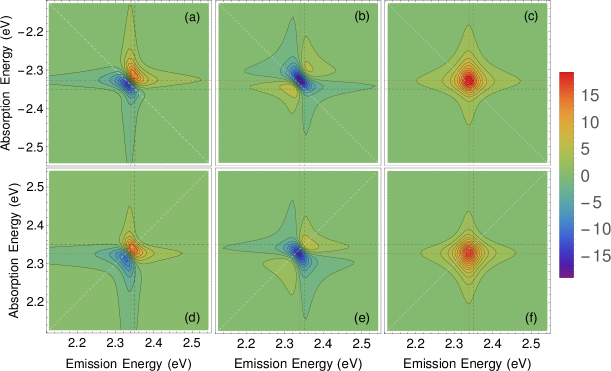
Figure 1: Rephasing (top) and non-rephasing (bottom) spectra at population time $t_{2}=100$ fs based on the SDE in Eq.(31). (a) and (d) are the real, (b) and (e) are the imaginary, (c) and (f) are the norm of the spectra. The parameters used in the simulation: $\hbar\omega=2.35$ eV, $\sigma=0.05~{}{\rm fs}^{-3/2}$, $\theta=0.01~{}{\rm fs}^{-1}$, and $\gamma_{0}=0.5~{}{\rm fs}^{-1}$.

II.2.2 Comparison to the Anderson-Kubo model and our previous excitation-induced dephasing (EID) theory

The well-known Anderson-Kubo theory describes the line shape broadening with regard to the stationary state of a random variable (usually the frequency fluctuation, $z_{t}$ here) characterized by an Ornstein-Uhlenbeck process. The expansion of the linear optical response function leads to the first cumulant $g_{1}^{\rm AK}(t)=\mu t$, in which $\mu$ is the drift term, i.e., the mean value, and the second cumulant

$$g_{2}^{\rm AK}(t)=\frac{\sigma^{2}}{2\theta^{3}}\left(e^{-\theta t}+\theta t-1\right).$$ (44)

In the short time limit $\theta t\ll 1$, the first cumulant in Eq. (40) turns to $g_{1}(t)\approx z_{0}t$, which has the same linear form as $g_{1}^{\rm AK}(t)$. It also agrees with the counterpart in our previous publication[4, 4]

$$g_{1}^{\rm EID}(t)=\frac{z_{0}}{2\theta}\left(1-e^{-2\theta t}\right)\approx z_{0}t.$$ (45)

It is worth noting that the relaxation rate here is $2\theta$ instead of $\theta$, because $\gamma(t)^{2}$ is the stochastic process of interest rather than $\gamma(t)$ characterized by the rate $\theta$. For deterministic initial condition, $z_{0}=\gamma_{0}^{2}/\omega^{2}$. The first cumulant $g_{1}(t)$ results in a red shift of $z_{0}\omega/2$ in the linear spectrum in the short time limit, which is determined by the initial average of the stochastic process $z(t)$.

When the initial fluctuation of $\gamma(t)$ obeys the same Ornstein-Uhlenbeck process, we conclude $\sigma_{\gamma_{o}}^{2}=\sigma^{2}/2\theta$ from the stationary state corresponding to the long-time limit where Eq. (34) turns into ${\rm Var}[\gamma(t)]=\sigma^{2}/2\theta$. Considering Eq. (61), we have

$$g_{1}(t)=\frac{\sigma^{2}}{2\theta\omega^{2}}t+\frac{\gamma_{0}^{2}}{2\theta\omega^{2}}\left(1-e^{-2\theta t}\right),$$ (46)

in which the second term looks similar to the $g_{1}^{\rm EID}(t)$ function in Eq. (45). However, $z_{0}=\gamma_{0}^{2}/\omega^{2}$ is true only for the deterministic initial condition, which is not the case in the above equation. Eq. (45) given in our previous publication leads to a time-dependent red shift that eventually vanishes after sufficiently long time. The first term then can be considered as a correction term that accounts for the interaction of paired-excitation and leads to a constant red shift of $\sigma^{2}/4\theta\omega$.

Therefore, the first cumulant of the present model produces the red shift similar to but more complex than the counterpart in our previous model, where interactions between paired-excitations are neglected. The initial frequency shift $z_{0}\omega/2$ agrees with the Anderson-Kubo theory, but converges to $\sigma^{2}/4\theta\omega$ rather than decaying to zero as in our previous papers.

Regarding the second cumulant, $g_{2}(t)$, the result from our previous work reads

$$g_{2}^{\rm EID}(t)=\frac{\sigma_{\gamma_{o}}^{2}}{\theta^{2}}\left(1-e^{-\theta t}\right)^{2}+\frac{\sigma^{2}}{2\theta^{3}}\left(2\theta t+4e^{-\theta t}-e^{-2\theta t}-3\right).$$ (47)

Compared to Eq. (41), the first term is recovered; however, the present model provides a more sophisticated description of the dependency on the initial average $z_{0}$.

In the limiting case of stationary state where $\sigma_{\gamma_{o}}^{2}=\sigma^{2}/2\theta$, the second cumulant in the present model turns into

$$g_{2}(t)=\frac{\sigma^{4}}{4\theta^{4}\omega^{4}}\left(e^{-2\theta t}+2\theta t-1\right)+\frac{\sigma^{2}\gamma_{0}^{2}}{\theta^{3}\omega^{4}}(e^{2\theta t}-2\theta t-1)e^{-2\theta t},$$ (48)

in which the first term reproduces the Anderson-Kubo lineshape but with half correlation time $\tau_{c}=(2\theta)^{-1}$ compared to that of the Anderson-Kubo theory $\theta^{-1}$. Furthermore, the second term gives the line broadening due to the initial average of the background exciton population, $\gamma_{0}^{2}$, which only results in a frequency shift in our previous model.

II.3 Inverting the spectral lineshape to extract the background process

The practical utility of any spectroscopic method is to extract information about the system or sample being interrogated. Any inversion approach will depend upon the model used for the input spectra and the model used to describe the coupling between the system and its environment. Here we consider the case in which the line-shape function follows from the Anderson-Kubo model, but the underlying background process is due to the pair fluctuation terms. From a spectroscopic point of view, we will have the typical motional narrowing and inhomogeneous broadening limits; however, their physical origins depend upon actual coupling to the background fluctuations. For this we consider just the stationary limit with the goal of relating the spectral lineshape to the underlying spectral density of the pair fluctuations.

Since $\gamma(t)=\omega\sqrt{z(t)}$ and we assume that $z(t)$ follows from an Ornstein-Uhlenbeck process, one has the SDE of $\gamma(t)$

$${\rm d}\gamma_{t}=-\left(\frac{\theta}{2}\gamma_{t}+\frac{\sigma^{2}\omega^{4}}{8}\gamma_{t}^{-3}\right){\rm d}t+\frac{\sigma\omega^{2}}{2}\gamma_{t}^{-1}{\rm d}W_{t},$$ (49)

with solution

$$\gamma(t)^{2}=\gamma(0)^{2}e^{-\theta t}+\sigma\omega^{2}\int_{0}^{t}e^{-\theta(t-\tau)}{\rm d}\tau.$$ (50)

Taking this to be a stationary process, we can integrate the SDE to find

$$\gamma(t)=\pm\omega\sigma^{1/2}\left[\int_{0}^{t}e^{-\theta(t-\tau)}{\rm d}W_{\tau}\right]^{1/2},$$ (51)

and use this to construct the spectral density of the underlying many-body dynamics.

$$S(\Omega)= \int_{-\infty}^{+\infty}{\rm d}t\langle\gamma_{t}\gamma_{0}\rangle e^{-i\Omega t}$$ (52)

However, since this involves taking averages over the Wiener process, we can not directly use the Itô identity ${\rm d}W^{2}_{t}={\rm d}t$ to perform the integration. We can, however, find the upper limit of the covariance according to Jensen’s inequality which relates the value of a convex function of an integral to the integral of the convex function[23, 24]. Here, taking $X$ as a random variable and $\varphi$ as a convex function, Jensen’s inequality gives

$$\phi(E[X])\leq E[\phi(X)].$$ (53)

This is essentially a statement that the secant line of a convex function lies above the graph of the function itself. As a corollary, the inequality is reversed for a concave function such as $\sqrt{x}$. In cases of stationary state or $\gamma(0)=0$, we have

$$\langle\gamma(t)\rangle\leq\omega\sigma^{1/2}\left<\int_{0}^{t}e^{-\theta(t-\tau)}{\rm d}W_{\tau}\right>^{1/2}=0,$$ (54)

which indicates that $\langle\gamma(t)\rangle=0$. The difference between the left and right sides of the inequality is termed the Jensen gap. Employing the inequality over a small integration range $\Delta t$

$$\langle\gamma(t+\Delta t)\gamma(t)\rangle\leq\frac{\sigma\omega^{2}}{\sqrt{2\theta}}e^{-\theta|\Delta t|/2}.$$ (55)

This then implies a spectral density of

$$S(\Omega)= \int_{-\infty}^{+\infty}{\rm d}t\langle\gamma_{t}\gamma_{0}\rangle e^{-i\Omega t}$$

$$\approx \frac{2\sqrt{2\theta}\sigma\omega^{2}}{\theta^{2}+\Omega^{2}}.$$ (56)

that can be well approximated by a Lorentzian in the limit that the Jensen inequality becomes an equality. Since the Lorentzian spectral density implies an underlying OU process for $\gamma_{t}$, in this limit the two cases considered here become identical. The equality is only satisfied when the convex (or concave) function is nearly linear over the entire given range of integration which implies that the $\theta\Delta t\gg 1$ in Eq. 56, corresponding to homogeneous or life-time limited broadening. We also have to conclude that the Jensen inequality can only be applied in one direction since starting from the assumption that $\gamma_{t}$ is a mean-reverting OU process gives the results presented in the previous section. This also would imply that care must be taken in interpreting the stationary lineshapes since the two different models for the background process appear to give similar spectral signatures.

If we specify the initial value of the coupling $\gamma(0)$ at $t=0$, we can use Jensen’s inequality to compute an upper limit of the covariance as

$$\langle\gamma(t),\gamma(s)\rangle\leq \frac{\sigma\omega^{2}}{\sqrt{2\theta}}\left[e^{-\theta|t-s|}-e^{-\theta(t+s)}\right]^{\frac{1}{2}}.$$ (57)

If we take both $t$ and $s$ at some later times such that the memory of the initial condition is lost and take $\Delta t=t-s$, we recover Eq. 55 as the stationary covariance.

In the non-stationary limit, however, the time-evolution of the mean (and hence $g_{1}(t)$) is very different. Using Mathematica, we were able to arrive at an analytical expression for $\langle\gamma(t)\rangle$ as given in the Appendix. Unlike its counterpart in the previous section, it does not relax exponentially to a stationary value and the resulting long-time value is far more complex. This suggests that one needs to look at both the line-shape and its temporal evolution to correctly extract the background dynamics.

III Discussion

In this paper, we further explore how the spectroscopic lineshape function reveals details of the electronic environment of an exciton. In particular, we consider the effect of pair excitations that arise from the full many-body expansion of the Bosonic Hamiltonian. As a simplifying assumption, we make the ansatz that these can be treated as a single classical variable that satisfies a known stochastic process, in this case the Ornstein-Uhlenbeck or Brownian motion process. We find that this does produce the lineshape function given by the Anderson-Kubo model, albeit with twice the coherence time. Importantly, we show that the model captures the formation of exciton/polarons as the steady-state/long-time limit. We also consider the reversed case where we assume that the frequency fluctuation obeys the Anderson-Kubo model and derive the underlying SDE for the pair-fluctuations and their spectral density. In this latter case, we show that working backwards from the stochastic frequency dynamics one can recover the the underlying spectral density in the long-time limit using the Jensen inequality.

The results from Sec.II.2 can be generalized for the case where the background process governing $\gamma(t)$ has a known spectral density that can be expressed as a series of exponential functions. Under this case, the $\gamma(t)$ is a sum over independent Ornstein-Uhlenbeck processes and thus, $z(t)$ will be a sum over independent processes. On the other hand, as discussed in Sec.II.3, inverting from an assumed process for $z(t)$ is non-trivial even for the rather simple model presented here; however, we can find an upper limit for the background spectral density governing $\gamma(t)$. While this can be taken simply as a mathematical exercise, we learn is that one can obtain from the lineshape a bound on the spectral density given a model system/bath interaction, but not the exact spectral density in all but specific cases. This is potentially a useful result for developing machine learning methods for spectral analysis.

We also believe that the approach can be extended to account for quantum noise effects by treating the $q\neq 0$ terms in Eq.5 as quantum noise terms rather than treating them as a collective classical variable. Furthermore, while our current approach is limited to bosonic excitations, it is possible to extend this approach to fermionic systems at finite temperature.

The cumulant expansion is a convenient technique to evaluate a function of random variables. For example, Bicout and Szabo’s work [25] provides a numerical strategy to compute the cumulant to arbitrary orders for a quadratically transformed stochastic process, namely passage through a fluctuating bottleneck, in its equilibrium/stationary distribution. It may be possible to extend our model to account for non-Markovian dynamics using the projection of multidimensional Markovian processes using their approach. Here, we truncate this expansion at the second cumulant, which is sufficient according to the Marcienkiewicz theorem [15, 16]. We emphasize that the non-stationarity of the dark-exciton background, and its dynamical coupling to the bright states, is a central component of the work presented here and could not be accounted for using a stationary picture as in Ref. 25.

Data Availability:The data that supports the findings of this study are available within the article.

Appendix A An alternative way to characterize $z(t)$

In Sec.II.2 we defined a transformed statistical process $z(t)=\gamma(t)^{2}/\omega^{2}$ to describe the relative frequency shift, which is attributed to the bi-excitation interaction characterized by $\gamma(t)$. Therefore, in principle, the statistical property of $z(t)$ can be derived from that of $\gamma(t)$. In this section, we will illustrate this approach by taking $\gamma(t)$ as an Ornstein-Uhlenbeck process, which is both Gaussian and Markovian. In the text we took the advantage of the Wiener process, using the Itô calculus, to solve $z(t)$ and its statistical property from the SDE. Here, we will make use of the statistical property of $\gamma(t)$ to find the mean value and autocorrelation function of $z(t)$, which are higher moments of $\gamma(t)$, using the property of the multivariate Gaussian distribution, without solving the SDE.

Let ${\bm{X}}=\{x_{1},x_{2},...,x_{N}\}^{\rm T}$ denote a set of Gaussian random variables with mean value vector ${\bar{\bm{X}}}=\{{\bar{x}_{1}},{\bar{x}_{2}},...,{\bar{x}_{N}}\}^{\rm T}$. The $k$-th moments read

$$\left<\prod_{j=1}^{N}\left(x_{j}-{\bar{x}}_{j}\right)^{r_{j}}\right>=\begin{dcases*}0,&if $k$ is odd,\\ \frac{(2\lambda)!}{\lambda!2^{\lambda}}\left\{\sigma_{jk}\sigma_{mn}...\right\}_{\rm sym},&if $k$ is even,\end{dcases*}$$ (58)

where $k=\sum_{j}r_{j}=2\lambda$. $\{...\}_{\rm sym}$ denotes the symmetric bilinear form on the Gaussian vector space. Being specific, it is the sum of the product of $\sigma$’s allocated into $\lambda$ pairs. The set of {$\sigma_{jk}=\langle x_{j},x_{k}\rangle\}$ forms the covariance matrix.

The Ornstein-Uhlenbeck process $\gamma(t)$ has the expected value

$$\langle\gamma(t)\rangle=\gamma_{0}e^{-\theta t},$$ (59)

where the initial average is $\gamma_{0}=\langle\gamma(0)\rangle$. We consider the Ornstein-Uhlenbeck process with indeterministic initial condition, therefore the covariance reads

$$\langle\gamma(t),\gamma(s)\rangle=\sigma_{\gamma_{o}}^{2}e^{-\theta(t+s)}+\frac{\sigma^{2}}{2\theta}\left[e^{-\theta|t-s|}-e^{-\theta(t+s)}\right],$$ (60)

where $\sigma_{\gamma_{o}}^{2}$ describes the fluctuation at time zero.

Before proceeding to the property of $z(t)$, we take a careful consideration about its initial condition. Since the average $z_{0}=\langle z(0)\rangle=\langle\gamma(0)^{2}\rangle/\omega^{2}$, one has

$$\omega^{2}z_{0}=\sigma_{\gamma_{o}}^{2}+\gamma_{0}^{2}.$$ (61)

Assuming the initial distribution of $\gamma(0)$ is Gaussian, one can use its fourth moment to find the fluctuation of $z(0)$

$$\omega^{4}\sigma_{z_{o}}^{2}=2\sigma_{\gamma_{o}}^{4}+4\sigma_{\gamma_{o}}^{2}\gamma_{0}^{2}.$$ (62)

The average of $z(t)$ can be found as

$$\left<z(t)\right> =\frac{1}{\omega^{2}}\left<\gamma(t)^{2}\right>$$

$$=\frac{\sigma_{\gamma_{o}}^{2}+\gamma_{0}^{2}}{\omega^{2}}e^{-2\theta t}+\frac{\sigma^{2}}{2\theta\omega^{2}}\left(1-e^{-2\theta t}\right),$$ (63)

which is exactly same as in Eq. (34) upon substitution of Eq. (61). Similarly, one finds the covariance

$$\left<z_{(}t),z(s)\right>= \frac{2\sigma_{\gamma_{o}}^{4}+4\sigma_{\gamma_{o}}^{2}\gamma_{0}^{2}}{\omega^{4}}e^{-2\theta(t+s)}+\frac{\sigma^{4}}{2\theta^{2}\omega^{4}}\left[e^{-\theta|t-s|}-e^{-\theta(t+s)}\right]^{2}+\frac{2\sigma^{2}}{\theta\omega^{4}}\left(\sigma_{\gamma_{o}}^{2}+\gamma_{0}^{2}\right)e^{-\theta(t+s)}\left[e^{-\theta|t-s|}-e^{-\theta(t+s)}\right].$$ (64)

Substituting Eqs. (61) and (62), one finds the the covariance given here to be identical as in Eq.(35).

Appendix B Changing variables using the Itô identity

We briefly review the change of variable procedure under Itô calculus. In general, we write a stochastic process as

$${\rm d}x=A[x]{\rm d}t+B[x]{\rm d}W_{t}$$ (65)

where $A[x]$ and $B[x]$ are both independent functions of the stochastic variable $x$ and time $t$ and $W_{t}$ is the Wiener process with ${\rm d}W_{t}^{2}={\rm d}t$ according to the Itô identity. Often, we need to cast a function the stochastic variable, $f[x(t)]$, in the form of an Itô stochastic equation. For this we need to perform a change of variables

$${\rm d}f[x] =f[x+dx]-f[x]$$

$$=f^{\prime}{\rm d}x+\frac{1}{2}f^{\prime\prime}{\rm d}^{2}\gamma+\cdots$$

$$=f^{\prime}\left(A[x]{\rm d}t+B[x]{\rm d}W\right)+\frac{1}{2}f^{\prime\prime}\left(A[x]{\rm d}t+B[x]{\rm d}W\right)^{2}$$

$$=(f^{\prime}A[x]+\frac{1}{2}f^{\prime\prime}B[x]^{2}){\rm d}t+f^{\prime}B[x]{\rm d}W_{t}$$ (66)

where $f^{\prime}$ and $f^{\prime\prime}$ denote partial derivatives of $f[x]$ respect to $x$. Under this, $f[x(t)]$ is considered as a transformed process with respect to the original $x(t)$ stochastic variable. It is straightforward to generalize this approach for vectors including correlation between stochastic terms. The reader is referred to Gardner’s excellent book for more details on stochastic methods and their applications.[26]

Appendix C Expression for $\langle\gamma(t)\rangle$ from Sec.II.3

We give here the expression derived for the expectation value of

$$\gamma(t)=\pm\omega\sigma^{1/2}\left[\int_{0}^{t}e^{-\theta(t-\tau)}{\rm d}W_{\tau}\right]^{1/2}$$ (67)

which is the solution of the Itô SDE

$${\rm d}\gamma_{t}=-\left(\frac{\theta}{2}\gamma_{t}+\frac{\sigma^{2}\omega^{4}}{8}\gamma_{t}^{-3}\right){\rm d}t+\frac{\sigma\omega^{2}}{2}\gamma_{t}^{-1}{\rm d}W_{t}.$$ (68)

Recall, that this is a transformed process in which we assumed that the observed frequency fluctuations were from an Ornstein-Uhlenbeck process with $\gamma(t)=\omega\sqrt{z(t)}$. Taking the initial value to be $z(0)=0$, one finds the average as

$$\langle\gamma(t);z(0)=0\rangle=\gamma_{eq}\frac{1}{(1-e^{-2\theta t})^{1/2}(\coth(\theta t)+1)^{3/4}}$$ (69)

with

$$\gamma_{eq}=\frac{\left(\frac{1}{2}+\frac{i}{2}\right)\omega}{\sqrt[4]{\theta}}\sqrt{\frac{\sigma}{\pi}}\Gamma\left(\frac{3}{4}\right)$$ (70)

which gives the red-shift of the exciton/polaron energy due to the pair-fluctuations. The $z(0)=0$ initial condition is of course a special case. Using Mathematica, one can arrive at a general expression for $\langle\gamma(t)\rangle$; however, as the expression is long and complicated we will not reproduce it here. The fact that $\gamma_{eq}$ can be complex-valued poses no difficulties since, formally, we can equivalently write the Hamiltonian in Eq.2 as

$$H=\hbar\omega a^{\dagger}a+\gamma(t)a^{\dagger}a^{\dagger}+\gamma^{*}(t)aa.$$ (71)

with eigenvalues

$$\lim_{t\to\infty}\langle\tilde{\omega}\rangle \approx\sqrt{\omega^{2}-|\gamma_{eq}/\hbar|^{2}}.$$ (72)

It is important to point out that that while the eigenvalue $\tilde{\omega}(t)$ depends upon $\gamma(t)$, we have already specified its evolution via the linearization expansion in Eq.16 and by specifying $z(t)$ to be an Ornstein-Uhlenbeck process. What we find instead is that $\langle\gamma(t)\rangle$ relates to the physical evolution of the background fluctuation that can be inferred by assuming a specific spectral model for the line-shape.

Appendix D Expression of correlation functions $R_{\alpha}$ in Section II.2

The correlation function Eq.(43) can be written in terms of the stochastic variable $z(\tau)$ using Eq.(16). Carrying out cumulant expansion to the second order, we have

$$R_{n}(\tau_{3},\tau_{2},\tau_{1}) =\left(\frac{i}{\hbar}\right)^{3}\mu^{4}\exp\left[i\omega\sum_{j=1}^{3}(\pm)_{j}\tau_{j}\right]\ \exp\left[\sum_{n=1}^{\infty}\frac{(-i\omega/2)^{n}}{n!}\left<\sum_{j=1}^{3}(\pm)_{j}\int_{0}^{\tau_{j}}z(\tau){\rm d}\tau\right>_{\rm c}\right]$$

$$\approx\left(\frac{i}{\hbar}\right)^{3}\mu^{4}\exp\left[i\omega\sum_{j=1}^{3}(\pm)_{j}\tau_{j}\right]\exp\left[-\frac{i\omega}{2}\sum_{j=1}^{3}g_{1}(\tau_{j})\right]\exp\left[-\frac{\omega^{2}}{8}\sum_{i,j=1}^{3}(\pm)_{i}(\pm)_{j}g_{2}(\tau_{i},\tau_{j})\right],$$ (73)

where $g_{1}(\tau)$ is given by Eq.(40), and the two-time lineshape function is

$$g_{2}(\tau_{1},\tau_{2})= \int_{0}^{\tau_{1}}\int_{0}^{\tau_{2}}\langle z(\tau),z(\tau^{\prime})\rangle{\rm d}\tau{\rm d}\tau^{\prime}$$

$$= \frac{\sigma_{z_{o}}^{2}}{4\theta^{2}}\left(1-e^{-2\theta\tau_{1}}\right)\left(1-e^{-2\theta\tau_{2}}\right)+\frac{\sigma^{2}z_{0}}{2\theta^{3}\omega^{2}}\left\{1-e^{-2\theta(\tau_{1}+\tau_{2})}-2e^{-2\theta\min(\tau_{1},\tau_{2})}+[1-2\theta\min(\tau_{1},\tau_{2})]\left(e^{-2\theta\tau_{1}}+e^{-2\theta\tau_{2}}\right)\right\}$$

$$+\frac{\sigma^{4}}{8\theta^{4}\omega^{4}}\left[e^{-2\theta(\tau_{1}+\tau_{2})}-e^{-2\theta|\tau_{2}-\tau_{1}|}+4e^{-2\theta\min(\tau_{1},\tau_{2})}-4+4\theta\min(\tau_{1},\tau_{2})\left(e^{-2\theta\tau_{1}}+e^{-2\theta\tau_{2}}+1\right)\right].$$ (74)

Appendix E Concerning the unitary transformation to diagonalize Eq.6

In our derivations we employed a very useful technique to bring the Hamiltonian in Eq. 6 to diagonal form. We give a quick review here for the interested reader. Writing $H$ in terms of diagonal and non-diagonal terms

$$H=H_{o}+W$$ (75)

one can easily show one can transform $H$ into a diagonal via

$$\tilde{H}=e^{-S}He^{S}$$ (76)

in which the operator $S$ is related to $H_{o}$ and $W$ via

$$[H_{o},S]=-W.$$ (77)

This last step is obtained by expanding the exponential. Having $S$, one now defines the transformed operators $\tilde{a}$ and $\tilde{a}^{\dagger}$ using a equations of motion approach such that

$$a(\tau)=e^{-S\tau}ae^{S\tau}$$ (78)

with $a(0)=a$ and $a(1)=\tilde{a}$ for all operators. Taking derivatives, one obtains Heisenberg equations

$$\partial_{\tau}a(\tau)=[a,S]$$ (79)

which can be integrated to give the results and transformed variables in the paper. For the case at hand, with $H_{o}=\hbar\omega(a^{\dagger}a+1/2)$, $W=\hbar\gamma(a^{\dagger}a^{\dagger}+aa)/2$, and $S=\xi(a^{\dagger}a^{\dagger}-aa)/2$ satisfies the condition in Eq. 77 and one obtains

$$\partial_{\tau}a(\tau) =-\gamma(t)a^{\dagger}(\tau)$$ (80)

$$\partial_{\tau}a^{\dagger}(\tau) =-\gamma(t)a(\tau)$$ (81)

Note that $\gamma(t)$ is time-dependent, the variable $\tau$ is not chronological time, it is simply introduced at each chronological-time and does not interfere with the time-ordering or integration over the stochastic variable $\gamma(t)$. Requiring the transformed $\tilde{H}$ to be diagonal yields the results around Eq. 6.

References

- W. Anderson [1954] P. W. Anderson, “A mathematical model for the narrowing of spectral lines by exchange or motion,” Journal of the Physical Society of Japan 9, 316–339 (1954), https://doi.org/10.1143/JPSJ.9.316 .
- Kubo [1954] R. Kubo, “Note on the stochastic theory of resonance absorption,” Journal of the Physical Society of Japan 9, 935–944 (1954), https://doi.org/10.1143/JPSJ.9.935 .
- Hamm and Zanni [2011] P. Hamm and M. Zanni, Concepts and Methods of 2D Infrared Spectroscopy (Cambridge University Press, 2011).
- Li et al. [2020] H. Li, A. R. Srimath Kandada, C. Silva, and E. R. Bittner, “Stochastic scattering theory for excitation-induced dephasing: Comparison to the anderson–kubo lineshape,” The Journal of Chemical Physics 153, 154115 (2020), https://doi.org/10.1063/5.0026467 .
- Srimath Kandada et al. [2020] A. R. Srimath Kandada, H. Li, F. Thouin, E. R. Bittner, and C. Silva, “Stochastic scattering theory for excitation-induced dephasing: Time-dependent nonlinear coherent exciton lineshapes,” The Journal of Chemical Physics 153, 164706 (2020), https://doi.org/10.1063/5.0026351 .
- Katsch, Selig, and Knorr [2020] F. Katsch, M. Selig, and A. Knorr, “Exciton-scattering-induced dephasing in two-dimensional semiconductors,” Phys. Rev. Lett. 124, 257402 (2020).
- [7] D. Erkensten, S. Brem, and E. Malic, “Excitation-induced dephasing in 2D materials and van der Waals heterostructures,” ArXiv:2006.08392 [cond-mat.mtrl-sci].
- Srimath Kandada and Silva [2020] A. R. Srimath Kandada and C. Silva, “Exciton polarons in two-dimensional hybrid metal-halide perovskites,” J. Phys. Chem. Lett. 11, 3173–3184 (2020).
- Siemens et al. [2010] M. E. Siemens, G. Moody, H. Li, A. D. Bristow, and S. T. Cundiff, “Resonance lineshapes in two-dimensional Fourier transform spectroscopy,” Optics Express 18, 17699–17708 (2010).
- Bristow et al. [2011] A. D. Bristow, T. Zhang, M. E. Siemens, S. T. Cundiff, and R. Mirin, “Separating homogeneous and inhomogeneous line widths of heavy-and light-hole excitons in weakly disordered semiconductor quantum wells,” J. Phys. Chem. B 115, 5365–5371 (2011).
- Skinner and Hsu [1986] J. L. Skinner and D. Hsu, “Pure dephasing of a two-level system,” The Journal of Physical Chemistry 90, 4931–4938 (1986), https://doi.org/10.1021/j100412a013 .
- Reichman, Silbey, and Suárez [1996] D. Reichman, R. J. Silbey, and A. Suárez, “On the nonperturbative theory of pure dephasing in condensed phases at low temperatures,” The Journal of Chemical Physics 105, 10500–10506 (1996), https://doi.org/10.1063/1.472976 .
- Born [1926] M. Born, “Quantenmechanik der stoßvorgänge,” Zeitschrift für Physik 38, 803–827 (1926).
- Wagner [1986] M. Wagner, Unitary Transformations in Solid State Physics, Modern problems in condensed matter sciences (North-Holland, 1986).
- Marcinkiewicz [1939] J. Marcinkiewicz, “Sur une propriété de la loi de Gauß,” Mathematische Zeitschrift 44, 612–618 (1939).
- Rajagopal and Sudarshan [1974] A. K. Rajagopal and E. C. G. Sudarshan, “Some generalizations of the marcinkiewicz theorem and its implications to certain approximation schemes in many-particle physics,” Phys. Rev. A 10, 1852–1857 (1974).
- Srimath Kandada et al. [2022] A. R. Srimath Kandada, H. Li, E. R. Bittner, and C. Silva-Acuña, “Homogeneous optical line widths in hybrid ruddlesden-popper metal halides can only be measured using nonlinear spectroscopy,” The Journal of Physical Chemistry C 126, 5378–5387 (2022), https://doi.org/10.1021/acs.jpcc.2c00658 .
- Fuller and Ogilvie [2015] F. D. Fuller and J. P. Ogilvie, “Experimental implementations of two-dimensional fourier transform electronic spectroscopy,” Annu. Rev. Phys. Chem. 66, 667–690 (2015).
- Cho [2008] M. Cho, “Coherent two-dimensional optical spectroscopy,” Chem. Rev. 108, 1331–1418 (2008).
- Tokmakoff [2000] A. Tokmakoff, “Two-dimensional line shapes derived from coherent third-order nonlinear spectroscopy,” J. Phys. Chem. A 104, 4247–4255 (2000).
- Li et al. [2006] X. Li, T. Zhang, C. N. Borca, and S. T. Cundiff, “Many-body interactions in semiconductors probed by optical two-dimensional fourier transform spectroscopy,” Phys. Rev. Lett. 96, 057406 (2006).
- Mukamel [1995] S. Mukamel, Principles of nonlinear optical spectroscopy, Vol. 6 (Oxford university press New York, 1995).
- Jensen [1906] J. L. W. V. Jensen, “Sur les fonctions convexes et les inégalités entre les valeurs moyennes,” Acta. Mathematica 30, 175–193 (1906).
- Handy, Littlewood, and Polya [1988] G. H. Handy, J. E. Littlewood, and G. Polya, Inequalities, 2nd ed. (Cambridge University Press, Cambridge, UK, 1988).
- Bicout and Szabo [1998] D. J. Bicout and A. Szabo, “Escape through a bottleneck undergoing non-markovian fluctuations,” The Journal of Chemical Physics 108, 5491–5497 (1998), https://doi.org/10.1063/1.475937 .
- Gardner [2009] C. Gardner, Stochastic Methods-A Handbook for the Natural and Social Sciences, 4th ed., Springer Series in Synergetics (Springer, Berlin, Heidelberg, 2009).