Non-isothermal diffusion in interconnected discrete-distributed systems: a variational approach

Abstract

Motivated by compartmental analysis in engineering and biophysical systems, we present a variational framework for the nonequilibrium thermodynamics of systems involving both distributed and discrete (finite dimensional) subsystems by specifically using the ideas of interconnected systems. We focus on the process of non-isothermal diffusion and show how the resulting form of the entropy equation naturally yields phenomenological expressions for the diffusion and entropy fluxes between two compartments, which results in generalized forms of Robin type interface conditions.

Keywords: Variational formulation, Lagrangian systems, interconnected systems, nonequilibrium thermodynamics, distributed systems, non-isothermal diffusion.

1 Introduction

Compartment modeling is a standard technique in the study of the dynamics of engineering or biophysical systems. In the simplest situations, each compartment can be efficiently described by homogeneous thermodynamic quantities, thus giving rise to a finite dimensional interconnected thermodynamic system. Some studies, for instance in intracellular dynamics, however require certain compartments to be considered as spatially distributed subsystems, while others can still be treated via a finite dimensional description. In this case, one needs to describe the thermodynamics of an interconnected discrete-distributed system, where the idea of interconnections, originally developed by Kron [1963] plays a key role in modeling such complicated systems.

In this paper we present a unified variational framework for the nonequilibrium thermodynamics of such interconnected systems based on the variational formulation for nonequilibrium thermodynamics developed in Gay-Balmaz and Yoshimura [2017a, b, 2019]. This formulation extends the Hamilton principle of classical mechanics to incorporate irreversible processes in both discrete (finite dimensional) and continuum systems. It consists of a critical action condition subject to two types of constraints:

• a phenomenological constraint imposed on the critical curve;

• a variational constraint imposed on the variations to be considered in the action functional.

The phenomenological constraint is directly constructed from the expression of the entropy production written in terms of the thermodynamic fluxes and forces involved in the systems (De Groot and Mazur [1969]). The phenomenological and variational constraints are systematically related thanks to the introduction of the concept of thermodynamic displacement associated to an irreversible process, defined such that its time rate of change equals the thermodynamic force of the process, Gay-Balmaz and Yoshimura [2017a, b, 2019]. From a mathematical point of view, this variational formulation appears as a nonlinear generalization of the Lagrange-d’Alembert principle of nonholonomic mechanics.

An important property of this variational formulation for the present work is the similar form that it takes for both discrete (finite dimensional) and continuum systems, which allows to naturally treat interconnected discrete-distributed systems. Our paper is structured as follows. In §2 we review the case of non-isothermal diffusion in interconnected discrete systems. In this case, one entropy variable and one molar variable can be associated to each subsystem. The second law naturally yields phenomenological relations given by the discrete analogue to the Fourier and Fick laws, and their cross-effects. In §3 we consider the case of a system involving both discrete and distributed compartments. The same type of variational formulation also applies in this case, both in its finite dimensional and continuum versions. For these systems, the Fourier and Fick laws and their cross-effects naturally appear in their usual continuum version as well as in a discrete form when associated to the transfer between the two compartments, thereby yielding Robin type interface condition. Finally, the case of interconnected distributed compartments is considered in §4.

2 Interconnected discrete systems

In this section we review from Gay-Balmaz and Yoshimura [2019] the variational formulation for the dynamics of non-isothermal diffusion between discrete interconnected compartments. In such a discrete description it is assumed that each compartment is well-stirred so that spatially uniform thermodynamic quantities can be attributed to each of them. The systems considered here are useful for the nonequilibrium thermodynamic description of membrane transport in biophysical systems, Oster, Perelson, and Katchalsky [1973]; Katchalsky and Curran [1975].

We assume that there is a single species and denote by $N_{A}$ and $S_{A}$ the number of moles and the entropy of the species in the compartment $A$, $A=1,....,K$. The internal energies are given as $U_{A}(S_{A},N_{A})$, where we assume that the volume of each compartment is constant, see Fig. 1. The variational formulation is based on the concept of thermodynamic displacement associated to an irreversible process, defined such that its time rate of change equals the thermodynamic force of the process. In our case, the thermodynamic force are the temperatures $T^{A}=\frac{\partial U_{A}}{\partial S_{A}}$ and chemical potentials $\mu^{A}=\frac{\partial U_{A}}{\partial N_{A}}$, so the thermodynamic displacements are variables $\Gamma^{A}$ and $W^{A}$ with

$$\dot{\Gamma}^{A}=T^{A}\qquad\text{and}\qquad\dot{W}^{A}=\mu^{A}.$$

We also introduce the entropy variables $\Sigma_{A}$ whose physical interpretation will be clarified later.

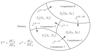
Figure 1: The heat and matter exchanger

The interfaces are assumed to be diathermal and permeable. We denote by $\mathcal{J}^{A\rightarrow B}$ the molar flow rate from compartment $A$ to compartment $B$ due to diffusion of the species, where $\mathcal{J}^{A\rightarrow B}=-\mathcal{J}^{B\rightarrow A}$. We also introduce the fluxes $J_{AB}$ with $J_{AB}=J_{BA}$ and such that $\sum_{B}J_{AB}=0$, for all $A$, associated to the total power exchange between compartments $A$ and $B$.

2.1 Variational formulation

Given a Lagrangian $L$ depending on all the variables, the variational formulation for this class of systems is

$$\delta\int_{t_{0}}^{t_{1}}\Big{[}L(S_{1},...,S_{K},N_{1},...,N_{K})$$ (1)

$$\hskip 42.67912pt+\sum_{A}\dot{W}^{A}N_{A}+\sum_{A}\dot{\Gamma}^{A}(S_{A}-\Sigma_{A})\Big{]}{\rm d}t=0$$

subject to

$$\frac{\partial L}{\partial S_{A}}\dot{\Sigma}_{A} =\sum_{B}J_{AB}\dot{\Gamma}^{B}+\sum_{B}\mathcal{J}^{B\rightarrow A}\dot{W}^{A},$$ (2)

$$\frac{\partial L}{\partial S_{A}}\delta\Sigma_{A} =\sum_{B}J_{AB}\delta\Gamma^{B}+\sum_{B}\mathcal{J}^{B\rightarrow A}\delta W^{A},$$

for $A=1,...,K$, with $\delta W^{A}|_{t=t_{0},t_{1}}=\delta\Gamma^{A}|_{t=t_{0},t_{1}}=0$.

2.2 Equations of evolution

From (1)–(2), one directly obtains the conditions

$$\delta N_{A}: \;\;\frac{\partial L}{\partial N_{1}}=-\dot{W}^{A} \;\;\delta S_{A}: \;\;\frac{\partial L}{\partial S_{A}}=-\dot{\Gamma}^{A}$$

$$\delta W^{A}: \;\;\dot{N}_{A}=\sum_{B}\mathcal{J}^{B\rightarrow A} \;\;\delta\Gamma^{A}: \;\;\dot{S}_{A}=\dot{\Sigma}_{A}+\sum_{B}J_{AB},$$

for $A=1,...,K$. Therefore, from $\sum_{B}J_{AB}=0$ one gets

$$\left\{\begin{array}[]{l}\vspace{0.2cm}\displaystyle\dot{N}_{A}=\sum_{B}\mathcal{J}^{B\rightarrow A}\\[5.69054pt] \vspace{0.2cm}\displaystyle\frac{\partial L}{\partial S_{A}}\dot{S}_{A}=-\sum_{B}J_{AB}\left(\frac{\partial L}{\partial S_{B}}-\frac{\partial L}{\partial S_{A}}\right)-\sum_{B}\mathcal{J}^{B\rightarrow A}\frac{\partial L}{\partial N_{A}}.\end{array}\right.$$ (3)

For the particular case of the Lagrangian

$$L(S_{1},...,S_{K},N_{1},...,N_{K})=-\sum_{A}U_{A}(S_{A},N_{A})$$

given by the sum of the internal energies for each compartments the evolution equations (3) become

$$\left\{\begin{array}[]{l}\vspace{0.2cm}\displaystyle\dot{N}_{A}=\sum_{B}\mathcal{J}^{B\rightarrow A}\\[5.69054pt] T^{A}\dot{S}_{A}=-\sum_{B}J_{AB}(T^{B}-T^{A})-\sum_{B}\mathcal{J}^{B\rightarrow A}\mu^{A},\end{array}\right.$$ (4)

together with $\dot{\Gamma}^{A}=T^{A}$, $\dot{W}^{A}=\mu^{A}$, and $\dot{\Sigma}_{A}=\dot{S}_{A}$.

2.3 Balance equations

From these evolution equations, it consistently follows that the total energy and number of moles are preserved while the total entropy $S=\sum_{A}S_{A}$ satisfies

$$\dot{S} =\sum_{A<B}\left(\frac{1}{T^{B}}-\frac{1}{T^{A}}\right)J_{AB}(T^{B}-T^{A})+\sum_{A<B}\left(\frac{\mu^{B}}{T^{B}}-\frac{\mu^{A}}{T^{A}}\right)\mathcal{J}^{B\rightarrow A},$$

which dictates the choice of phenomenological expressions for $J_{AB}$ and $\mathcal{J}^{B\rightarrow A}$ in accordance with the second law of thermodynamics, see Gay-Balmaz and Yoshimura [2019]. For instance, in the linear regime, these expressions read

$$\begin{bmatrix}\vspace{0.2cm}J_{AB}\frac{T^{A}-T^{B}}{T^{A}T^{B}}\\ \vspace{0.1cm}\mathcal{J}^{B\rightarrow A}\\ \end{bmatrix}=\mathcal{L}_{AB}\begin{bmatrix}\vspace{0.2cm}T^{B}-T^{A}\\ \vspace{0.1cm}\frac{\mu^{B}}{T^{B}}-\frac{\mu^{A}}{T^{A}}\\ \end{bmatrix},$$ (5)

where the symmetric part of $2\times 2$ matrix $\mathcal{L}^{AB}=\mathcal{L}^{BA}$ is positive, for all $A,B=1,...,K$. The entries of these matrices are phenomenological coefficients which may in general depend on the state variables. From Onsager’s relation, the matrices $\mathcal{L}^{AB}$ are symmetric for all $A,B$. The phenomenological expressions in (5) describe the discrete version of the Fourier and Fick laws, as well as their cross-effects given by discrete versions of the Soret and Dufour effects. Assuming that the Lagrangian can be written as the sum $\sum_{A}L_{A}(S_{A},N_{A})$ of Lagrangians associated to each compartment, the balance of energy of the subsystem given by the compartment $A$ is found as

$$\frac{d}{dt}E_{A}=\sum_{B}J_{AB}(T^{A}-T^{B}),\quad A=1,...,K.$$

This allows to relate $J_{AB}$ to the power exchange between compartments $A$ and $B$ as $J_{AB}(T^{A}-T^{B})=P^{B\rightarrow A}$.

The extension of the variational formulation (1)-(2) to the case of an open system exchanging matter and heat with the exterior is presented in Gay-Balmaz and Yoshimura [2018a], while the case of reacting systems is developed in Gay-Balmaz and Yoshimura [2022]. The approach developed here directly applies to non-isothermal versions of the diffusion through composite membranes presented in Kedem and Katchalsky [1963a].

3 Interconnected discrete-distributed systems

We consider here the case of non-isothermal diffusion in a system made from discrete (well-stirred) as well as spatially distributed compartments. Such a situation is important in applications where homogenization techniques can be applied to some compartments to reduce the complexity of the system and the computational cost. For instance, in some studies of intracellular dynamics, the cellular and nuclear membranes must be considered as spatially distributed subdomains while homogenization techniques can be applied to the cytoplasm and the nucleus, see, e.g. Chaudhry [2012] and references therein.

For simplicity, we consider one well-stirred discrete compartment and one $n$-dimensional spatially distributed compartment, where the discrete compartment is assumed to have no interaction with the exterior. We denote by $\Omega\subset\mathbb{R}^{n}$, $n=1,2,3$ the domain of the well-stirred compartment, assumed to be compact with piecewise smooth boundary. The boundary $\partial\Omega$ splits into two parts, namely the exterior boundary $\partial\Omega^{e}$ and the interior boundary $\partial\Omega^{i}$ which is in contact with the well-stirred compartment, see Fig. 2.

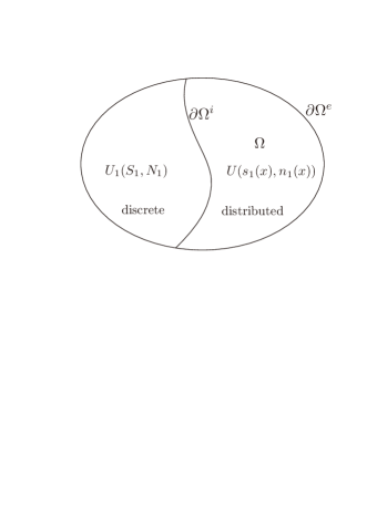
Figure 2: The interconnected distributed-discrete system

3.1 Variational formulation

Let us denote by $S$ and $N$ the entropy and the number of moles in the discrete compartment and by $s(x)$ and $n(x)$ the entropy density and mole number density in the distributed compartment $\Omega$ with $x\in\Omega$. We consider a general, possibly mixed discrete-distributed, Lagrangian function of the form $\mathscr{L}(S,N,s,n)$. We will denote by $\delta\mathscr{L}/\delta s$ and $\delta\mathscr{L}/\delta n$ the functional derivatives of $\mathscr{L}$ with respect to the density variables, defined by

$$\left.\frac{d}{d\varepsilon}\right|_{\varepsilon=0}\mathscr{L}(S,N,s+\varepsilon\delta s,n)=\int_{\Omega}\frac{\delta\mathscr{L}}{\delta s}\delta s{\rm d}x,$$

$$\left.\frac{d}{d\varepsilon}\right|_{\varepsilon=0}\mathscr{L}(S,N,s,n+\varepsilon\delta n)=\int_{\Omega}\frac{\delta\mathscr{L}}{\delta n}\delta n{\rm d}x,$$

for arbitrary $\delta s_{1}$ and $\delta n_{1}$. Such functional derivatives are assumed to exist. If the Lagrangian is of the form

$$\mathscr{L}(S,N,s,n)=L(S,N)+\int_{\Omega}\mathcal{L}(s,n){\rm d}x$$ (6)

with $L(S,N)$ the Lagrangian of the discrete compartment and $\mathcal{L}(s,n)$ the Lagrangian density of the distributed compartment, then one has $\delta\mathscr{L}/\delta s=\partial\mathcal{L}/\partial s$ and $\delta\mathscr{L}/\delta n=\partial\mathcal{L}/\partial n$.

We denote by $\mathbf{j}_{s}$ and $\mathbf{j}$ and entropy flux and diffusive flux densities. By merging the variational setting for discrete thermodynamic systems (see §2 and Gay-Balmaz and Yoshimura [2019]) and for continuum thermodynamic systems (see Gay-Balmaz and Yoshimura [2017b, 2019]), we get the following variational formulation

$$\delta\int_{t_{0}}^{t_{1}}\!\Big{[}\mathscr{L}(S,N,s,n)+\dot{W}N+\dot{\Gamma}(S-\Sigma)$$ (7)

$$\hskip 56.9055pt+\int_{\Omega}\big{(}\partial_{t}w\,n+\partial_{t}\gamma\,(s-\sigma)\big{)}{\rm d}x\Big{]}{\rm d}t=0$$

subject to the phenomenological constraints

$$\frac{\partial\mathscr{L}}{\partial S}\dot{\Sigma} =\int_{\partial\Omega^{i}}\left(\dot{\Gamma}+\frac{\delta\mathscr{L}}{\delta s}\biggr{|}_{\partial\Omega^{i}}\right)\,\mathbf{j}_{s}\cdot\mathbf{n}\,{\rm d}\mathsf{A}$$ (8)

$$\qquad\qquad+\int_{\partial\Omega^{i}}\left(\dot{W}+\frac{\delta\mathscr{L}}{\delta n}\biggr{|}_{\partial\Omega^{i}}\right)\,\mathbf{j}\cdot\mathbf{n}\,{\rm d}\mathsf{A},$$

$$\frac{\delta\mathscr{L}}{\delta s}\partial_{t}\sigma =\mathbf{j}_{s}\cdot\nabla\partial_{t}\gamma+\mathbf{j}\cdot\nabla\partial_{t}w,$$

and the variational constraints

$$\frac{\partial\mathscr{L}}{\partial S}\delta\Sigma =\int_{\partial\Omega^{i}}\delta\Gamma\,\mathbf{j}_{s}\cdot\mathbf{n}\,{\rm d}\mathsf{A}+\int_{\partial\Omega^{i}}\delta W\,\mathbf{j}\cdot\mathbf{n}\,{\rm d}\mathsf{A},$$ (9)

$$\frac{\delta\mathscr{L}}{\delta s}\delta\sigma =\mathbf{j}_{s}\cdot\nabla\delta\gamma+\mathbf{j}\cdot\nabla\delta w,$$

where $\mathbf{n}$ denotes the outward pointing unit normal vector field to $\partial\Omega$, ${\rm d}\mathsf{A}$ is the area element on $\partial\Omega$, and where $\delta W,\delta\Gamma,\delta w,\delta\gamma$ vanish at $t=t_{0},t_{1}$ and $\delta w|_{\partial\Omega}=\delta\gamma|_{\partial\Omega}=0$. In the above, we introduce the thermodynamic displacements $W$, $\Gamma$ and the thermodynamic displacement densities $w$, $\gamma$ and we also employ the internal entropy $\Sigma$ and the internal entropy density $\sigma$. One passes from the phenomenological constraints to the variational constraints by replacing the time rate of change of the thermodynamic displacements with $\delta$-variations (such as $\dot{\Gamma}\leadsto\delta\Gamma$) and by removing the affine terms, as usual for constraints of thermodynamic type, Gay-Balmaz and Yoshimura [2018a].

3.2 Equations of evolution

Taking the variation of the integral in (7) and using $\delta W|_{t=t_{0},t_{1}}=\delta\Gamma|_{t=t_{0},t_{1}}=0$ and $\delta w|_{t=t_{0},t_{1}}=\delta\gamma|_{t=t_{0},t_{1}}=0$, we get

$$\begin{split}&\int_{t_{0}}^{t_{1}}\Big{[}\frac{\partial\mathscr{L}}{\partial N}\delta N+\frac{\partial\mathscr{L}}{\partial S}\delta S+\delta N\dot{W}-\dot{N}\delta W-(\dot{S}-\dot{\Sigma})\delta\Gamma+\delta S\dot{\Gamma}-\delta\Sigma\dot{\Gamma}\\[5.69054pt] &\quad+\int_{\Omega}\Big{(}\frac{\delta\mathscr{L}}{\delta s}\delta s+\frac{\delta\mathscr{L}}{\delta n}\delta n+\delta n\partial_{t}w-\partial_{t}n\delta w\\[5.69054pt] &\qquad\qquad\qquad-(\partial_{t}s-\partial_{t}\sigma)\delta\gamma+\delta s\partial_{t}\gamma-\delta\sigma\partial_{t}\gamma\Big{)}{\rm d}x\Big{]}{\rm d}t=0.\end{split}$$

Since the variations $\delta N$, $\delta S$, $\delta n$, and $\delta s$ are free, one has

$$\begin{split}\delta N:&\;\;\frac{\partial\mathscr{L}}{\partial N}=-\dot{W},\quad\;\;\;\,\delta S:\;\;\frac{\partial\mathscr{L}}{\partial S}=-\dot{\Gamma},\\[5.69054pt] \delta n:&\;\;\frac{\delta\mathscr{L}}{\delta n}=-\partial_{t}w,\quad\;\;\delta s:\;\;\frac{\delta\mathscr{L}}{\delta s}=-\partial_{t}\gamma.\end{split}$$

From this, the previous condition becomes

$$\begin{split}&\int_{t_{0}}^{t_{1}}\Big{[}-\dot{N}\delta W-(\dot{S}-\dot{\Sigma})\delta\Gamma+\delta\Sigma\frac{\partial\mathscr{L}}{\partial S}\\[5.69054pt] &+\int_{\Omega}\Big{(}-\partial_{t}n\delta w-(\partial_{t}s-\partial_{t}\sigma)\delta\gamma+\delta\sigma\frac{\delta\mathscr{L}}{\delta s}\Big{)}{\rm d}x\Big{]}{\rm d}t=0.\end{split}$$

Using now the variational constraint (9) and $\delta w|_{\partial\Omega}=\delta\gamma|_{\partial\Omega}=0$, we get

$$\delta W: \;\;\dot{N}=\int_{\partial\Omega^{i}}\mathbf{j}\cdot\mathbf{n}\,{\rm d}{\mathsf{A}} \;\;\delta\Gamma: \;\;\dot{\Sigma}=\dot{S}-\int_{\partial\Omega^{i}}\mathbf{j}_{s}\cdot\mathbf{n}\,{\rm d}\mathsf{A}$$

$$\delta w: \;\;\partial_{t}n+\operatorname{div}\mathbf{j}=0 \;\;\delta\gamma: \;\;\partial_{t}\sigma=\partial_{t}s+\operatorname{div}\mathbf{j}_{s}.$$

To summarize we have obtained the evolution equations

$$\left\{\begin{array}[]{l}\vspace{0.3cm}\displaystyle\dot{N}=\int_{\partial\Omega^{i}}\mathbf{j}\cdot\mathbf{n}\,{\rm d}{\mathsf{A}},\qquad\partial_{t}n+\operatorname{div}\mathbf{j}=0\\ \vspace{0.3cm}\displaystyle\frac{\partial\mathscr{L}}{\partial S}\Big{(}\dot{S}-\int_{\partial\Omega^{i}}\!\!\mathbf{j}_{s}\cdot\mathbf{n}\,{\rm d}\mathsf{A}\Big{)}\\ \vspace{0.3cm}\displaystyle\quad=\int_{\partial\Omega^{i}}\!\!\Big{(}\!-\frac{\partial\mathscr{L}}{\partial S}+\frac{\delta\mathscr{L}}{\delta s}\biggr{|}_{\partial\Omega^{i}}\Big{)}\,\mathbf{j}_{s}\cdot\mathbf{n}\,{\rm d}\mathsf{A}\\ \vspace{0.3cm}\displaystyle\qquad+\int_{\partial\Omega^{i}}\Big{(}-\frac{\partial\mathscr{L}}{\partial N}+\frac{\delta\mathscr{L}}{\delta n}\biggr{|}_{\partial\Omega^{i}}\Big{)}\,\mathbf{j}\cdot\mathbf{n}\,{\rm d}\mathsf{A}\\[5.69054pt] \displaystyle\frac{\delta\mathscr{L}}{\delta s}(\partial_{t}s+\operatorname{div}\mathbf{j}_{s})=-\mathbf{j}_{s}\cdot\nabla\frac{\delta\mathscr{L}}{\delta s}-\mathbf{j}\cdot\nabla\frac{\delta\mathscr{L}}{\delta n}.\end{array}\right.$$ (10)

When $\mathscr{L}$ is given by (6) with $L(S,N)=-U(S,N)$ the internal energy of the discrete compartment and $\mathcal{L}(s,n)=-u(s(x),n(x))$ the internal energy density of the distributed compartment, we introduce $T:=\dot{\Gamma}=-\frac{\partial\mathscr{L}}{\partial S}=\frac{\partial U}{\partial S}$, $\mathcal{M}:=\dot{W}=-\frac{\partial\mathscr{L}}{\partial N}=\frac{\partial U}{\partial N}$, $\tau:=\partial_{t}\gamma=-\frac{\delta\mathscr{L}}{\delta s}=\frac{\partial u}{\partial s}$, $\mu:=\partial_{t}w=-\frac{\delta\mathscr{L}}{\delta n}=\frac{\partial u}{\partial n}$. Hence, the last two equations in (10) read

$$\left\{\begin{array}[]{l}\vspace{0.2cm}\displaystyle T\Big{(}\dot{S}-\int_{\partial\Omega^{i}}\mathbf{j}_{s}\cdot\mathbf{n}\,{\rm d}\mathsf{A}\Big{)}=\int_{\partial\Omega^{i}}\Big{(}\tau|_{\partial\Omega^{i}}-T\Big{)}\,\mathbf{j}_{s}\cdot\mathbf{n}\,{\rm d}\mathsf{A}\\ \vspace{0.3cm}\displaystyle\hskip 113.81102pt+\int_{\partial\Omega^{i}}\Big{(}\mu|_{\partial\Omega^{i}}-\mathcal{M}\Big{)}\,\mathbf{j}\cdot\mathbf{n}\,{\rm d}\mathsf{A},\\ \displaystyle\tau(\partial_{t}s+\operatorname{div}\mathbf{j}_{s})=-\mathbf{j}_{s}\cdot\nabla\tau-\mathbf{j}\cdot\nabla\mu.\end{array}\right.$$

3.3 Balance equations

The mole balance of the distributed compartment can be written as

$$\frac{d}{dt}\int_{\Omega}n\,{\rm d}x=-\int_{\partial\Omega^{i}}\mathbf{j}\cdot\mathbf{n}\,{\rm d}\mathsf{A}-\int_{\partial\Omega^{e}}\mathbf{j}\cdot\mathbf{n}\,{\rm d}\mathsf{A}$$

which shows the contributions associated with the exchanges across the interior and exterior boundaries. From this and the first equation in (10), the total mole balance reads

$$\frac{d}{dt}\left[N+\int_{\Omega}n\,{\rm d}x\right]=-\int_{\partial\Omega^{e}}\mathbf{j}\cdot\mathbf{n}\,{\rm d}\mathsf{A}.$$

The entropy balances for the discrete and distributed compartments are found as

$$\begin{split}\dot{S}&=\frac{1}{T}\int_{\partial\Omega^{i}}\Big{(}\tau|_{\partial\Omega^{i}}-T\Big{)}\,\mathbf{j}_{s}\cdot\mathbf{n}\,{\rm d}\mathsf{A}\\ &\quad\underbrace{\quad+\frac{1}{T}\int_{\partial\Omega^{i}}\Big{(}\mu|_{\partial\Omega^{i}}-\mathcal{M}\Big{)}\,\mathbf{j}\cdot\mathbf{n}\,{\rm d}\mathsf{A}}_{=\mathfrak{I}_{\partial\Omega^{i}}}+\underbrace{\int_{\partial\Omega^{i}}\mathbf{j}_{s}\cdot\mathbf{n}\,{\rm d}\mathsf{A}}_{=\mathcal{J}_{S}^{\rm int}}\end{split}$$

and

$$\begin{split}\frac{d}{dt}\int_{\Omega}s\,{\rm d}x&=\underbrace{-\int_{\Omega}\frac{1}{\tau}\,\mathbf{j}_{s}\cdot\nabla\tau\,{\rm d}x-\int_{\Omega}\frac{1}{\tau}\,\mathbf{j}\cdot\nabla\mu\,{\rm d}x}_{=\mathfrak{I}_{\Omega}}\\ &\quad-\underbrace{\int_{\partial\Omega^{i}}\mathbf{j}_{s}\cdot\mathbf{n}\,{\rm d}\mathsf{A}}_{=\mathcal{J}_{S}^{\rm int}}-\underbrace{\int_{\partial\Omega^{e}}\mathbf{j}_{s}\cdot\mathbf{n}\,{\rm d}\mathsf{A}}_{=-\mathcal{J}_{S}^{\rm ext}},\end{split}$$

where we denote by $\mathfrak{I}_{\partial\Omega^{i}}$ and $\mathfrak{I}_{\Omega}$ the entropy generation rate for each compartment. We also denote by $\mathcal{J}_{S}^{\rm int}$ the entropy flow rate from the distributed to the discrete compartment and by $\mathcal{J}_{S}^{\rm ext}$ the entropy flow rate from the exterior to the distributed compartment. In addition, note that

$$\mathfrak{I}_{\partial\Omega^{i}}=\dot{\Sigma}\qquad\text{and}\qquad\mathfrak{I}_{\Omega}=\frac{d}{dt}\int_{\Omega}\sigma\,{\rm d}x$$

which show that the entropy generation rates coincide with the time rate of change of the variables $\Sigma$ and $\sigma$. This attributes a clear physical meaning to these two entropy variables appearing in the variational formulation (7)-(9). The total entropy balance thus reads

$$\frac{d}{dt}\left[S+\int_{\Omega}s\,{\rm d}x\right]=\mathfrak{I}_{\partial\Omega^{i}}+\mathfrak{I}_{\Omega}+\mathcal{J}_{S}^{\rm ext},$$

where the internal entropy flow rate $\mathcal{J}_{S}^{\rm int}$ cancels out.

The energy balances for each compartment are

$$\begin{split}\dot{U}&=\int_{\partial\Omega^{i}}\big{(}\tau|_{\partial\Omega^{i}}\mathbf{j}_{s}+\mu|_{\partial\Omega^{i}}\mathbf{j}\big{)}\cdot\mathbf{n}\,{\rm d}\mathsf{A},\\ \frac{d}{dt}\int_{\Omega}u\,{\rm d}x&=-\int_{\partial\Omega}\big{(}\tau|_{\partial\Omega}\mathbf{j}_{s}+\mu|_{\partial\Omega}\mathbf{j}\big{)}\cdot\mathbf{n}\,{\rm d}\mathsf{A}\end{split}$$

so that the total energy balance is found as

$$\frac{d}{dt}\left[U+\int_{\Omega}u\,{\rm d}x\right]=-\int_{\partial\Omega^{e}}\big{(}\tau|_{\partial\Omega^{e}}\mathbf{j}_{s}+\mu|_{\partial\Omega^{e}}\mathbf{j}\big{)}\cdot\mathbf{n}\,{\rm d}\mathsf{A}=P^{\rm ext},$$

where we recall that the boundary $\partial\Omega$ of the distributed compartment splits into the internal $\partial\Omega^{i}$ and external $\partial\Omega^{e}$ boundaries and $P^{\rm ext}$ is the heat and matter power exchange from the exterior to the system. Since the discrete compartment is assumed to have no interaction with the exterior, the system is adiabatically closed if $\mathbf{j}_{s}\cdot\mathbf{n}=\mathbf{j}\cdot\mathbf{n}=0$ on $\partial\Omega^{e}$. The extension to the case where the discrete compartment can also exchanges heat and matter with the exterior can be achieved by appropriately combining the variational formulation (7)–(9) with the approach developed in Gay-Balmaz and Yoshimura [2018a].

3.4 Phenomenology

From the second law and the expressions found for $\mathfrak{I}_{\Omega}$ and $\mathfrak{I}_{\Omega_{i}}$, the resulting form of entropy production suggests, in the linear regime, the phenomenological relations

$$-\begin{bmatrix}\vspace{0.2cm}\mathbf{j}_{s}\\ \mathbf{j}\\ \end{bmatrix}=\begin{bmatrix}\vspace{0.2cm}\mathcal{L}_{ss}&\mathcal{L}_{sn}\\ \mathcal{L}_{ns}&\mathcal{L}_{nn}\\ \end{bmatrix}\begin{bmatrix}\vspace{0.2cm}\nabla\tau\\ \nabla\mu\\ \end{bmatrix}\qquad\text{on}\qquad\Omega,$$ (11)

and

$$\begin{bmatrix}\vspace{0.2cm}\mathbf{j}_{s}\!\cdot\mathbf{n}\\ \mathbf{j}\cdot\mathbf{n}\\ \end{bmatrix}=\begin{bmatrix}\vspace{0.2cm}\ell_{ss}&\ell_{sn}\\ \ell_{ns}&\ell_{nn}\\ \end{bmatrix}\begin{bmatrix}\vspace{0.2cm}\tau|_{\partial\Omega^{i}}-T\\ \mu|_{\partial\Omega^{i}}-\mathcal{M}\\ \end{bmatrix}\quad\text{on}\quad\partial\Omega^{i},$$ (12)

for state functions $\mathcal{L}_{ss},\mathcal{L}_{sn},\mathcal{L}_{ns},\mathcal{L}_{nn}$ and $\ell_{ss},\ell_{sn},\ell_{ns},\ell_{nn}$ such that the symmetric parts of the $2\times 2$ matrices are positive. In the diagonal case one gets the relations

$$\begin{split}&\mathbf{j}_{s}=-\mathcal{L}_{ss}\nabla T\text{ on }\Omega,\,-\mathcal{L}_{ss}\nabla T\cdot\mathbf{n}=\ell_{ss}\big{(}\tau|_{\partial\Omega^{i}}\!-\!T\big{)}\text{ on }\partial\Omega^{i},\\[5.69054pt] &\mathbf{j}=-\mathcal{L}_{nn}\nabla\mu\text{ on }\Omega,-\mathcal{L}_{nn}\nabla n\cdot\mathbf{n}=\ell_{nn}\big{(}\mu|_{\partial\Omega^{i}}\!-\!\mathcal{M}\big{)}\text{ on }\partial\Omega^{i},\end{split}$$

thereby giving Robin type of boundary conditions for heat and matter transfer through the internal boundary.

3.5 One-dimensional case

As a simple instance of the variational approach developed in this section, we consider a one dimensional distributed compartment $\Omega=[0,D]\subset\mathbb{R}$ as illustrated in Fig. 3.

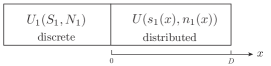
Figure 3: The interconnected 1D distributed-discrete system

The variational formulation reduces to

$$\delta\int_{t_{0}}^{t_{1}}\!\Big{[}\mathscr{L}(S,N,s,n)+\dot{W}N+\dot{\Gamma}(S-\Sigma)$$ (13)

$$\qquad\qquad+\int_{0}^{D}\big{(}\partial_{t}w\,n+\partial_{t}\gamma\,(s-\sigma)\big{)}{\rm d}x\Big{]}{\rm d}t=0$$

subject to

$$\frac{\partial\mathscr{L}}{\partial S}\dot{\Sigma} =-\left(\dot{\Gamma}+\frac{\delta\mathscr{L}}{\delta s}\biggr{|}_{0}\right)\,j_{s}\biggr{|}_{0}-\left(\dot{W}+\frac{\delta\mathscr{L}}{\delta n}\biggr{|}_{0}\right)j\biggr{|}_{0},$$ (14)

$$\frac{\delta\mathscr{L}}{\delta s}\partial_{t}\sigma =j_{s}\partial_{x}\partial_{t}\gamma+j\partial_{x}\partial_{t}w,$$

and

$$\frac{\partial\mathscr{L}}{\partial S}\delta\Sigma =-\delta\Gamma j_{s}\bigr{|}_{0}-\delta Wj\bigr{|}_{0},$$ (15)

$$\frac{\delta\mathscr{L}}{\delta s}\delta\sigma =j_{s}\partial_{x}\delta\gamma+j\partial_{x}\delta w,$$

with $\delta w|_{\partial\Omega}=\delta\gamma|_{\partial\Omega}=0$, where $j_{s}|_{0}$ and $j|_{0}$ denotes the boundary values at $x=0$. This formulation is obtained from (7)–(9) by noting that the terms $\int_{\partial\Omega^{i}}\mathbf{j}\cdot\mathbf{n}\,{\rm d}\mathsf{A}$ and $\int_{\partial\Omega^{e}}\mathbf{j}\cdot\mathbf{n}\,{\rm d}\mathsf{A}$ correspond to $-j|_{0}$ and $j|_{D}$, respectively, similarly for $\mathbf{j}_{s}$ and $j_{s}$.

For the Lagrangian (6) in which $L$ and $\mathcal{L}$ are given by the internal energies $U(S,N)$ and $u(s(x),n(x))$, we get from (13)–(15) the evolution equations:

$$\left\{\begin{array}[]{l}\vspace{0.2cm}\displaystyle\dot{N}=-j|_{0},\qquad\partial_{t}n+\partial_{x}j=0,\\[5.69054pt] \vspace{0.2cm}\displaystyle T\big{(}\dot{S}+j_{s}|_{0}\big{)}\!=\!-\big{(}\tau|_{0}-T\big{)}j_{s}|_{0}-\big{(}\mu|_{0}-\mathcal{M}\big{)}j|_{0},\\[5.69054pt] \displaystyle\tau(\partial_{t}s+\partial_{x}j_{s})\!=\!-j_{s}\partial_{x}\tau-j\partial_{x}\mu.\end{array}\right.$$ (16)

The various balances equations are easily deduced from this system. In particular, the total energy and entropy balances take the following form

$$\begin{split}&\frac{d}{dt}\left[S+\int_{0}^{D}s\,{\rm d}x\right]=-\frac{1}{T}\big{(}\tau|_{0}-T\big{)}j_{s}|_{0}-\frac{1}{T}\big{(}\mu|_{0}-\mathcal{M}\big{)}j_{s}|_{0}\\ &\qquad\quad-\int_{0}^{D}\frac{1}{\tau}j_{s}\partial_{x}\tau\,{\rm d}x-\int_{0}^{D}\frac{1}{\tau}j\partial_{x}\mu\,{\rm d}x+j_{s}|_{D},\\[5.69054pt] &\frac{d}{dt}\left[U+\int_{0}^{D}u\,{\rm d}x\right]=-\tau|_{D}j_{s}|_{D}-\mu|_{D}j|_{D}.\end{split}$$

4 Interconnected distributed systems

We consider here the case of a domain $\Omega$ made from several interconnected distributed compartments $\Omega_{A}$, $A=1,...,K$. We denote by $\Sigma_{AB}=\partial\Omega_{A}\cap\partial\Omega_{B}$ the interface between compartments $A$ and $B$ and by $\partial\Omega_{A}^{e}=\partial\Omega\cap\Omega_{A}$ the external boundary of compartment $\Omega_{A}$. Let $\mathbf{j}_{A,s}$ and $\mathbf{j}_{A}$ be the entropy and diffusive flux densities in compartment $A$ and let $\mathbf{n}_{A}$ be the outward pointing unit normal vector field to $\partial\Omega_{A}$. The mass flux and energy flux continuity conditions across $\Sigma_{AB}$ imply

$$(\mathbf{j}_{A}-\mathbf{j}_{B})\cdot\mathbf{n}_{A}=0,$$ (17)

$$\big{(}(T^{A}\mathbf{j}_{A,s}+\mu^{A}\mathbf{j}_{A})-(T^{B}\mathbf{j}_{B,s}+\mu^{B}\mathbf{j}_{B})\big{)}\cdot\mathbf{n}_{A}=0$$

on $\Sigma_{AB}$.

For a given Lagrangian functional $\mathscr{L}(s_{1},...,s_{K},n_{1},...,n_{K})$, the continuum version of the variational formulation yields

$$\delta\int_{t_{0}}^{t_{1}}\Big{[}\mathscr{L}(s_{1},...,s_{K},n_{1},...,n_{K})$$ (18)

$$\;+\sum_{A}\int_{\Omega_{A}}\big{(}\partial_{t}w^{A}n_{A}+\partial_{t}\gamma^{A}(s_{A}-\sigma_{A})\big{)}{\rm d}x\Big{]}{\rm d}t=0$$

subject to

$$\frac{\delta\mathscr{L}}{\delta s_{A}}\partial_{t}\sigma_{A} =\mathbf{j}_{A,s}\cdot\nabla\partial_{t}\gamma^{A}+\mathbf{j}_{A}\cdot\nabla\partial_{t}w^{A},$$ (19)

and

$$\frac{\delta\mathscr{L}}{\delta s_{A}}\delta\sigma^{A} =\mathbf{j}_{A,s}\cdot\nabla\delta\gamma^{A}+\mathbf{j}_{A}\cdot\nabla\delta w^{A},$$ (20)

for $A=1,...,K$.

4.1 Equations of evolution

Since the computation of the critical condition is similar to the one presented above for the distributed compartment, we directly present the resulting conditions. We get

$$\begin{split}\delta n_{A}:&\;\;\frac{\delta\mathscr{L}}{\delta n_{A}}=-\partial_{t}w^{A},\;\;\delta s_{A}:\;\;\frac{\delta\mathscr{L}}{\delta s_{A}}=-\partial_{t}\gamma^{A}\\[5.69054pt] \delta w^{A}:&\;\;\partial_{t}n_{A}+\operatorname{div}\mathbf{j}_{A}=0,\;\;\delta\gamma^{A}:\;\;\partial_{t}\sigma_{A}=\partial_{t}s_{A}+\operatorname{div}\mathbf{j}_{A,s},\end{split}$$

for $A=1,...,K$, so that the final system equations read

$$\left\{\begin{array}[]{l}\vspace{0.15cm}\displaystyle\partial_{t}n_{A}+\operatorname{div}\mathbf{j}_{A}=0\\[5.69054pt] \vspace{0.15cm}\displaystyle\frac{\delta\mathscr{L}}{\delta s_{A}}(\partial_{t}s_{A}\!+\!\operatorname{div}\mathbf{j}_{A,s})\!=\!-\mathbf{j}_{A,s}\!\cdot\!\nabla\frac{\delta\mathscr{L}}{\delta s_{A}}\!-\!\mathbf{j}_{A}\!\cdot\!\nabla\frac{\delta\mathscr{L}}{\delta n_{A}},\end{array}\right.$$ (21)

for $A=1,...,K$.

For the Lagrangian functional $\mathscr{L}(s_{1},...,s_{K},n_{1},...,n_{K})=-\sum_{A}\int_{\Omega_{A}}u_{A}(s_{A},n_{A}){\rm d}x$, with $u_{A}$ the internal energy density of compartment $A$, we have

$$T^{A}\!:=\!-\frac{\delta\mathscr{L}}{\delta s_{A}}=\frac{\partial u_{A}}{\partial s_{A}}\;\;\textrm{and}\;\;\mu^{A}:=-\frac{\delta\mathscr{L}}{\delta n_{A}}=\frac{\partial u_{A}}{\partial n_{A}},$$

so that the last equation becomes

$$T^{A}(\partial_{t}s_{A}+\operatorname{div}\mathbf{j}_{A,s})=-\mathbf{j}_{A,s}\cdot\nabla T^{A}-\mathbf{j}_{A}\cdot\nabla\mu^{A}.$$

4.2 Balance equations

The mole balance for compartment $\Omega_{A}$ is

$$\frac{d}{dt}\int_{\Omega_{A}}n_{A}{\rm d}x=-\sum_{B}\int_{\Sigma_{AB}}\mathbf{j}_{A}\cdot\mathbf{n}_{A}\,{\rm d}\mathsf{A}-\int_{\partial\Omega^{e}_{A}}\mathbf{j}_{A}\cdot\mathbf{n}_{A}\,{\rm d}\mathsf{A},$$

which shows the contributions associated with the exchanges across $\Sigma_{AB}$ and $\partial\Omega_{A}^{e}$. From the first condition in (17), the total mole balance reads

$$\frac{d}{dt}\sum_{A}\int_{\Omega_{A}}n_{A}{\rm d}x=-\sum_{A}\int_{\partial\Omega^{e}_{A}}\mathbf{j}_{A}\cdot\mathbf{n}_{A}\,{\rm d}\mathsf{A}.$$

The total entropy balance is computed as

$$\frac{d}{dt}\sum_{A}\int_{\Omega_{A}}s_{A}{\rm d}x$$

$$=\sum_{A}\int_{\Omega_{A}}\Big{[}-\operatorname{div}\mathbf{j}_{s,A}-\frac{1}{T^{A}}\mathbf{j}_{s,A}\cdot\nabla T^{A}-\frac{1}{T^{A}}\mathbf{j}_{A}\cdot\nabla\mu^{A}\Big{]}{\rm d}x$$

$$=-\sum_{A}\underbrace{\int_{\Omega_{A}}\Big{[}\frac{1}{T^{A}}\mathbf{j}_{s,A}\cdot\nabla T^{A}+\frac{1}{T^{A}}\mathbf{j}_{A}\cdot\nabla\mu^{A}\Big{]}{\rm d}x}_{=-\mathfrak{I}_{\Omega_{A}}}$$

$$\quad+\sum_{A<B}\underbrace{\int_{\Sigma_{AB}}(\mathbf{j}_{B,s}-\mathbf{j}_{A,s})\cdot\mathbf{n}_{A}\,{\rm d}\mathsf{A}}_{\mathfrak{I}_{\Sigma_{AB}}}-\sum_{A}\underbrace{\int_{\partial\Omega_{A}^{e}}\mathbf{j}_{A,s}\cdot\mathbf{n}_{A}\,{\rm d}\mathsf{A}}_{=-\mathcal{J}_{S}^{{\rm ext}\rightarrow A}},$$

where $\mathfrak{I}_{\partial\Omega_{A}}$ and $\mathfrak{I}_{\Sigma_{AB}}$ are the entropy generation rate for each compartment and interface. We have also identified the entropy flow rate $\mathcal{J}_{S}^{{\rm ext}\rightarrow A}$ from exterior to the distributed compartment $\Omega_{A}$. We finally note the equality

$$\mathfrak{I}_{\Omega_{A}}=\frac{d}{dt}\int_{\Omega_{A}}\sigma_{A}{\rm d}x,$$

which relates $\sigma_{A}$ to the entropy generation in $\Omega_{A}$. The energy balances for each compartment reads

$$\frac{d}{dt}\!\int_{\Omega_{A}}\!\!u_{A}{\rm d}x=-\sum_{B}\int_{\Sigma_{AB}}\!\!\big{(}T^{A}|_{\Sigma_{AB}}\mathbf{j}_{A,s}\!+\!\mu^{A}|_{\Sigma_{AB}}\mathbf{j}_{A}\big{)}\!\cdot\!\mathbf{n}_{A}\,{\rm d}\mathsf{A}$$

$$-\int_{\partial\Omega_{A}^{e}}\big{(}T^{A}|_{\partial\Omega_{A}^{e}}\mathbf{j}_{A,s}+\mu^{A}|_{\partial\Omega_{A}^{e}}\mathbf{j}_{A}\big{)}\cdot\mathbf{n}_{A}\,{\rm d}\mathsf{A}$$

$$=\sum_{B}P^{B\rightarrow A}+P^{{\rm ext}\rightarrow A},$$

where we have identified the power exchanges from $\Omega_{B}$ to $\Omega_{A}$ and from the exterior to $\Omega_{A}$. Using the second condition (17) we have $P^{B\rightarrow A}=-P^{A\rightarrow B}$ so that the total energy balance is found as

$$\frac{d}{dt}\sum_{A}\int_{\Omega_{A}}u_{A}\,{\rm d}x$$

$$=-\sum_{A}\int_{\partial\Omega_{A}^{e}}\big{(}T^{A}|_{\partial\Omega_{A}^{e}}\mathbf{j}_{A,s}+\mu^{A}|_{\partial\Omega_{A}^{e}}\mathbf{j}_{A}\big{)}\cdot\mathbf{n}_{A}\,{\rm d}\mathsf{A}=P^{\rm ext}.$$

4.3 Phenomenology

From the second law and the expressions for $\mathfrak{I}_{\partial\Omega_{A}}$ and $\mathfrak{I}_{\Sigma_{AB}}$, we must have

$$-\mathbf{j}_{s,A}\cdot\nabla T^{A}-\mathbf{j}_{A}\cdot\nabla\mu^{A}\geq 0\quad\text{and}\quad(\mathbf{j}_{B,s}-\mathbf{j}_{A,s})\cdot\mathbf{n}_{A}\geq 0.$$

Using the two relations (17), the second condition is

$$\big{(}(T^{A}-T^{B})\mathbf{j}_{A,s}+(\mu^{A}-\mu^{B})\mathbf{j}_{A}\big{)}\cdot\mathbf{n}_{A}\geq 0.$$

This suggests, in the linear regime, the phenomenological relations

$$-\begin{bmatrix}\vspace{0.2cm}\mathbf{j}_{A,s}\\ \mathbf{j}_{A}\\ \end{bmatrix}=\begin{bmatrix}\vspace{0.2cm}\mathcal{L}^{A}_{ss}&\mathcal{L}^{A}_{sn}\\ \mathcal{L}^{A}_{ns}&\mathcal{L}^{A}_{nn}\\ \end{bmatrix}\begin{bmatrix}\vspace{0.2cm}\nabla T^{A}\\ \nabla\mu^{A}\\ \end{bmatrix}$$ (22)

on $\Omega_{A}$, for all $A=1,...,K$ and

$$\begin{bmatrix}\vspace{0.2cm}\mathbf{j}_{A,s}\!\cdot\mathbf{n}_{A}|_{\Sigma_{AB}}\\ \mathbf{j}_{A}\cdot\mathbf{n}_{A}|_{\Sigma_{AB}}\\ \end{bmatrix}=\begin{bmatrix}\vspace{0.2cm}\ell_{ss}^{AB}&\ell_{sn}^{AB}\\ \ell_{ns}^{AB}&\ell_{nn}^{AB}\\ \end{bmatrix}\begin{bmatrix}\vspace{0.2cm}T^{A}-T^{B}\\ \mu^{A}-\mu^{B}\\ \end{bmatrix}$$ (23)

on $\Sigma_{AB}$, for all $A<B$, where the symmetric parts of the $2\times 2$ are positive. As earlier, in the diagonal case one obtains Robin type interface conditions for heat and matter transfer.

4.4 Future work

We project to analyze further how the variational formulation presented here for the interconnected system can be systematically constructed from the variational formulation for each thermodynamic subsystem, in a similar way to the approach in Jacobs and Yoshimura [2014] for interconnection in Lagrangian mechanics.

References

• Chaudhry [2012] Chaudhry, Q. A. Computational Modeling of Reaction and Diffusion Processes in Mammalian Cell. PhD thesis, KTH, Stockholm, Sweden.
• De Groot and Mazur [1969] De Groot, S. R and P. Mazur Nonequilibrium Thermodynamics. North-Holland: New York, NY, USA, 1969.
• Jacobs and Yoshimura [2014] Jacobs, H. O. and H. Yoshimura. Tensor product of Dirac structures and interconnection in Lagrangian mechanics. J. Geom. Mech. 2014, 6(1), 67–98.
• Katchalsky and Curran [1975] Katchalsky, A. and P. F. Curran. Nonequilibrium Thermodynamics in Biophysics. Harvard University Press, Cambridge, Massachusetts, 1975.
• Kedem and Katchalsky [1963a] Kedem O. and A. Katchalsky. Permeability of composite membranes. Part 1. Electric current, volume flow and flow of solute through membranes. Trans. Faraday Soc. 1963, 59, 1918–1930.
• Kron [1963] Kron, G. Diakoptics: The piecewise solution of large-scale systems, McDonald, London, 1963.
• Gay-Balmaz and Yoshimura [2017a] Gay-Balmaz, F. and H. Yoshimura. A Lagrangian variational formulation for nonequilibrium thermodynamics. Part I: discrete systems. J. Geom. Phys. 111:169–193, 2017a.
• Gay-Balmaz and Yoshimura [2017b] Gay-Balmaz, F. and H. Yoshimura. A Lagrangian variational formulation for nonequilibrium thermodynamics. Part II: continuum systems. J. Geom. Phys., 111:194–212, 2017b.
• Gay-Balmaz and Yoshimura [2018a] Gay-Balmaz, F. and H. Yoshimura. A variational formulation of nonequilibrium thermodynamics for discrete open systems with mass and heat transfer. Entropy, 20(3):163, 2018.
• Gay-Balmaz and Yoshimura [2019] Gay-Balmaz, F. and H. Yoshimura. From Lagrangian mechanics to nonequilibrium thermodynamics: a variational perspective. Entropy, 21(1), 2019.
• Gay-Balmaz and Yoshimura [2022] Gay-Balmaz, F. and H. Yoshimura. Thermodynamics of non-isothermal reacting open systems: from variational to bracket formulations. preprint, 2022.
• Oster, Perelson, and Katchalsky [1973] Oster, G. F., A. S. Perelson, and A. Katchalsky. Network thermodynamics: Dynamic modelling of biophysical systems. Q. Rev. Biophys. 6, 1–134, 1973.