A Transformer-Based Contrastive Learning Approach for Few-Shot Sign Language Recognition

Abstract

Sign language recognition from sequences of monocular images or 2D poses is a challenging field, not only due to the difficulty to infer 3D information from 2D data, but also due to the temporal relationship between the sequences of information. Additionally, the wide variety of signs and the constant need to add new ones on production environments makes it infeasible to use traditional classification techniques. We propose a novel Contrastive Transformer-based model, which demonstrate to learn rich representations from body key points sequences, allowing better comparison between vector embedding. This allows us to apply these techniques to perform one-shot or few-shot tasks, such as classification and translation. The experiments showed that the model could generalize well and achieved competitive results for sign classes never seen in the training process.

Keywords Sign Language  $\cdot$ Transformers  $\cdot$ Contrastive Learning  $\cdot$ Few-shot Learning

1 Introduction

According to the World Health Organization (WHO), by the year of 2050 more than 700 million people will have disabling hearing loss. Currently, over five percent of the global population is deaf, which equates to more than 466 million people [1]. These deaf people, primarily, communicated using a group of spatiotemporal languages called Sign Languages [2]. Each country usually has its own sign language, with particular gestures and meaning. Libras (Brazilian Sign Language), for example, is the official sign language of Brazil [3], in other countries where they do not adopt any sign language as one of the official languages, they create public and educational policies such as the Individuals with Disabilities Education Act (IDEA) created by the United States [4] to address their needs.

Sign language is often understudied and makes use of gestures, which makes communication difficult to non-signers. This language barrier arises because the deaf usually do not master written language, and only a few hearing people can communicate using sign language [5]. Learners that were born deaf, typically, face great difficulties during the acquisition of reading and writing skills [6]. This is because Sign Language has notable differences in grammar, morphology, syntax and semantics. Commonly having completely different structures to express the same idea when comparing Sign Language with Written Language [7].

Several researches dealing with this theme and seeking solutions to overcome this communication barrier between a deaf person and a hearing person. Most of the works presented propose to solve the problem in the area of computer vision with machine learning, however, many works limit their advances as a consequence of the existing sign language datasets being limited to a small number of words [8] and these words are composed of low number of examples.

To address this problems with the recent advances in machine learning, deep learning models are used to perform the translation of sign language. In this paper, we propose a model consisting of a pose model to extract the key-points referring to body and hands for each frame and a Transformer to encode the sequentially of the key-points of the entire input video. One of the advantages of the Transformer is that it can pass the entire input sequence in a parallel way, unlike recurrent units like LSTM or GRU, where the input sequence must be passed step-by-step. The transformer also uses a mechanism of Self-Attention that allows for better performance in long sequences.

The model is then trained in a contrastive learning approach by using triplet loss. After that, the model can be used to map sequences of key-points semantically into vectors from an embedding vector space. This representation can be useful to perform tasks, such as classification by comparing the embedding vectors through nearest neighbor, cosine similarity, euclidean distance, etc. This way, the model will have the ability to compare new inputs to only a few examples of already known signs and perform classification by measuring the distance between them. This also allows it to classify inputs for new classes without the need for retraining.

The main contribution of this paper to sign language recognition is to present a novel way of perform classification tasks of isolated signals by using a Transformer encoder trained in a contrastive learning approach that need few examples.

The next sections are divided as follows: Section 2 presents the relevant works in the literature; Section 3 gives an overview of the theoretical background related to this paper; Section 4 shows the implementation; Section 5, experiments and results details. Finally, Section 5 presents the conclusions of the experiments and future works.

2 Related Works

Sign Language Recognition (SLR) can be divided into two main areas: single sign recognition, which refers to signs representing one concept or gloss and continuous sign recognition which is related to a continuous stream of signs for sentences and multiple glosses. This paper presents a way of classifying single signs.

Different approaches have been used to address the issue of sign recognition [9]. One of the first papers on SLR was published by [10]. They used recurrent neural networks (RNN) to recognize single signs from a sequence of symbols of a finger alphabet but could not perform sign segmentation in time, since it was trained on sign level. [11] and [12] trained a Fuzzy Min Max Neural Network (FMMNN) with 25 single signs and 131 words, respectively. Several authors also used Neural Networks (NN), such as [13], that combined the results of the training of different layers, each one trained in different level of sign abstraction, and [14] that used 2D motion trajectories to train a Time Delay Neural Network (TDNN) to recognize American Sign Language (ASL).

In the 90’s, Hidden Markov Models dominated the research [15, 16] given the similarity with speech recognition and the simplification of the temporal aspect of SLR. Furthermore, [17] used Deterministic Finite Automaton (DFA) to recognize Korean Sign Language (KSL), [18] used k-Nearest Neighbours (KNNs) and decision trees to classify single signs.

Since then, Deep Neural Networks have been largely used in SLR. [19] used a Convolutional Neural Networks (CNNs) to classify 20 Italian gestures with data from a Microsoft Kinect on fullbody images with information about depth, achieving 91.7% of accuracy. [20] proposed a 3D CNN where the third dimension corresponds to the frames in a video in order to recognize human actions. [21] used 3D CNNs to extract spatial and temporal features from sign language by integrating multiple sources of visual data.

Besides the problem of extracting visual information from each frame, it is also necessary to extract temporal information from a video in order to gain knowledge about the sequence of movements. For this, [22] proposed a Convolutional Recurrent Neural Network (C-RNN), where a CNN is combined to a RNN to address the contextual dependence between images. The C-RNN have been applied to SLR by [23] to classify signs from the ASL Dataset.

Transformer Networks [24] are relatively new and have achieved impressive results in Natural Language Processing (NLP) and Computer Vision tasks. In NLP, models such as BERT [25], were trained in a large corpus of text and achieved state-of-the-art results in many tasks, such as translation, text classification and question answering. [26] used Transformers recognize and locate human actions from a video by using a sequence of RGB frames as input.

Transformers are also present in SLR. [27] used a Transformer connected to a Connectionist Temporal Classification (CTC) to perform a continuous SLR and [28] could overcome inaccuracies in detection of skeleton key-points corruption.

Literature review shows that the recognition of single signs is usually implemented through a supervised classification task in which the model must be trained with a fixed number of classes and several labeled examples of each class. This approach is very expensive in terms of data acquisition and not scalable: a new class can only be incorporated by adding labeled examples of it and retraining of network. This problem is particularly critical in task such SLR, since it is common to deal with a tens of thousands of distinct signs.

Considering the scalability problem, [29] investigated the possibility of approaching SLR using few-shot learning techniques, such as Matching Networks, Model-Agnostic Meta-Learning and Prototypical Networks in very small datasets of electromyograms of sign language performance, obtaining interesting results. Additionally, the authors indicate the possibility of transfer learning from a sign language to another. [30] sought to go further by addressing the problem as zero-shot sign language recognition (ZSSLR) by training from a dataset composed by video of single signs paired with its respective textual description that works as an intermediate-level semantic representation for knowledge transfer. The descriptive text embedding emerged by training can describe unseen signs.

For this paper, we propose a method that achieved few-shot learning for single sign language recognition using a Transformer to encode the sequence of key-points from a video and performing the training with Triplet Loss, a method proposed by [31] that achieved state-of-the-art results in face recognition tasks. This method will be detailed in Sections 3 and 4.

3 Proposed Model

The pipeline proposed in this work consists of multiple steps that goes from the input video, as a sequence of RGB frames, to the predicted output class. First, the RGB images have their key-points extracted by a pose and hands model forming a skeleton of the person performing the sign. The sequence of skeletons is then passed to the Transformer encoder to predict the embedding of the sequence and, finally, a classification model will make the class prediction. The classification as the last step is necessary to perform few-shot learning. The architecture overview can be seen in Figure 1 and each step of the pipeline will be seen in this Section.

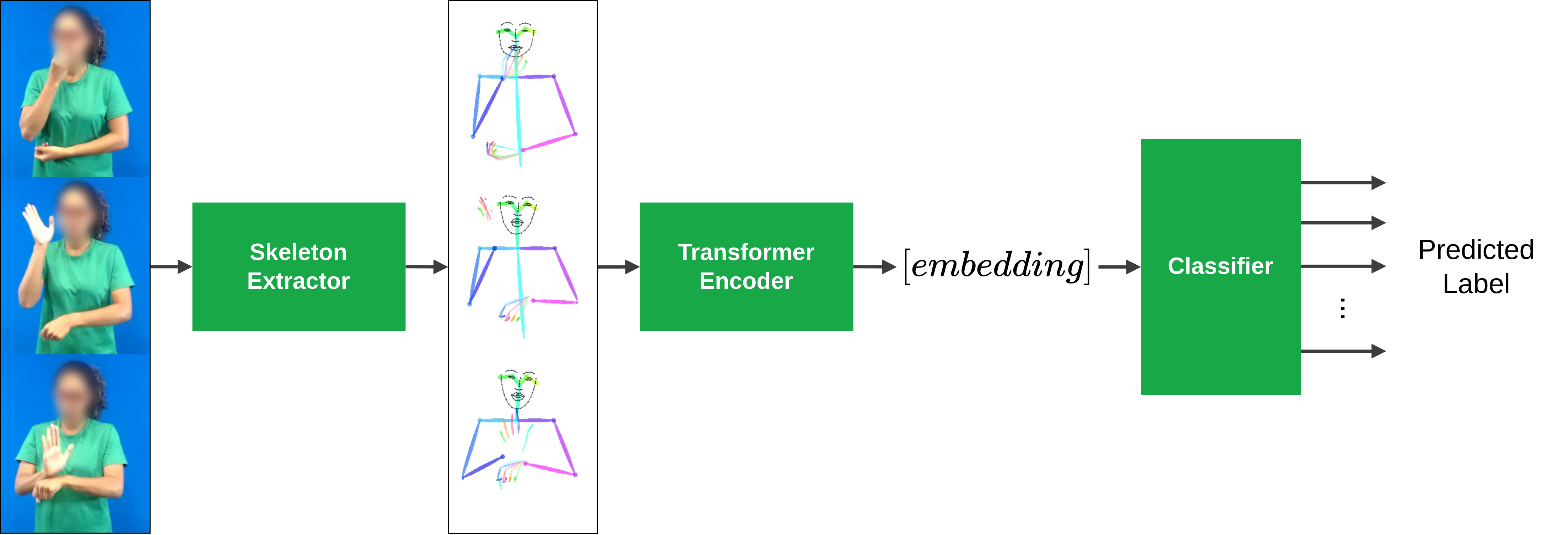
Figure 1: Proposed pipeline overview. The RGB images will be the input of a pose and hands (skeleton) model and then the Transformer encoder will predict the embedding representation of the input and in the last step, the classifier will predict the input class.

3.1 Skeleton Extraction

The sequence of RGB images from the input videos could be sent directly to the model as a collection of pixels for each one of the images color channels, such as Convolutional Neural Networks [32] or Image Transformers [33]. The complexity of a large quantity of pixels makes it necessary to have larger models, capable of creating good internal representations of the data in the context of the problem being solved [34]. For this, more data is required in order to prevent common problems such as overfitting (when the model adjusts itself exactly accordingly to its training data and fails to predict new results) or when occurs a shortcut (when the model relies on a simple characteristic of the training data rather than learning to represent the distribution of the real world scenario of the problem [35]). Additionally, given a limited training set and computer resources, the training process could have a poor performance and become difficult to converge.

To perform Sign Language Recognition, only the information related to the position of the body, hands and face are required, while other information contained in the pixels of the images, such as color, shadow and depth, should not affect the classification results. In order to extract this useful information, it is a good practice to use a pre-trained model to predict the key-points of the body, hands and face, such as [36] and [37]. The key-points are a set of coordinates that represents specific regions of the subject of interest, such as articulations, fingers or regions of the face.

However, in this work, MediaPipe Holistic [37] is used as a pre-trained key-point predictor to extract the skeleton from RGB images of pose and hands. MediaPipe Holistic consists of a pipeline of separate models for pose, face and hands, shown in Figure 2, where each model have specializations and have different input formats. The pose model receives a lower and fixed resolution image (256x256), but that resolution would be too low for the hand models, therefore, a multi-stage pipeline is used which treat the component using an appropriate resolution. The face model was not used in this experiments.

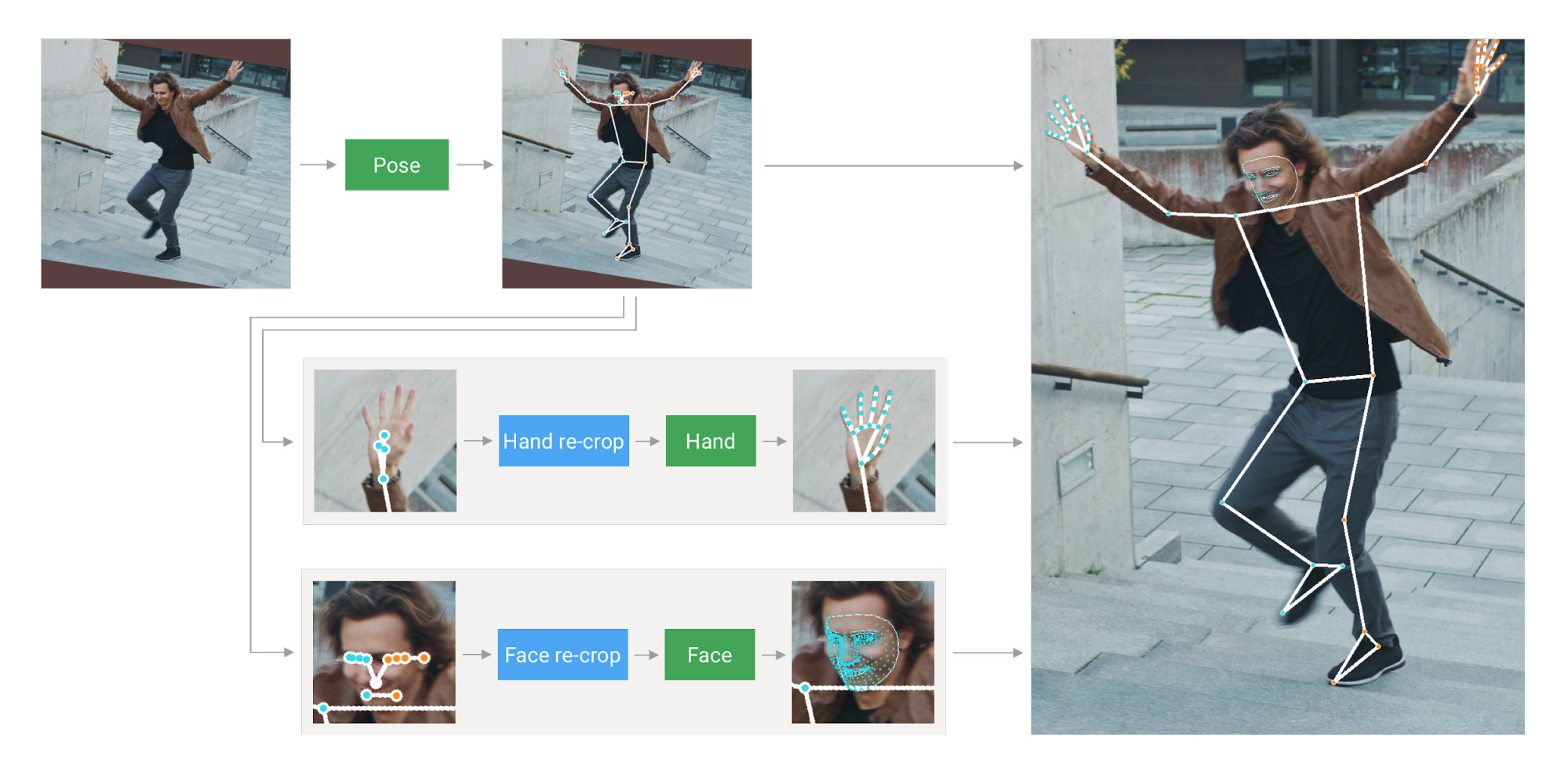
Figure 2: MediaPipe Holistic Overview (Source: [38]).

In this work, the skeleton is built from the pose, containing 33 key-points, and hands, each containing 21 key-points. The z-coordinate for each key-point is discarded. Therefore, the skeleton extractor model will receive an image as input and produces 2D coordinates pairs as outputs for each one of the $M$ joints that represents the body skeleton. For a sequence of frames $V$, the collection of extracted key-points will be $X=(X_{1},X_{2},X_{3},...,X_{N})$ where $X_{i}=(x^{1}_{i},y^{1}_{i},x^{2}_{i},y^{2}_{i},...,x^{M}_{i},y^{M}_{i})$ represents the collection of $(x_{i}^{k},y_{i}^{k})$ coordinates for the $k^{th}$ key-point of the $i^{th}$ frame and $N$ is the sequence length. Hence, $X\in\mathbb{R}^{2M}$.

Additionally, in order to remove any bias related to the dynamic aspects of sign such as speed, position and frame rate of cameras, an temporal interpolation is made in the skeleton sequences $X$ to standardize its length. The experiments conducted to evaluate this process are detailed in Section 5.

3.2 Transformer

The sequence of coordinates $X$ from a sequence of images $V$ will serve as input to a multi-layer Transformer encoder based on the implementation from [24]. As in BERT [25], the first element of every sequence is a special classification token, [CLS], in which its final hidden state is used as an accumulated sequence representation. This hidden state is used to make comparisons in the embedding space mapped by the model. The Transformer model with its inputs and outputs is shown in Figure 3.

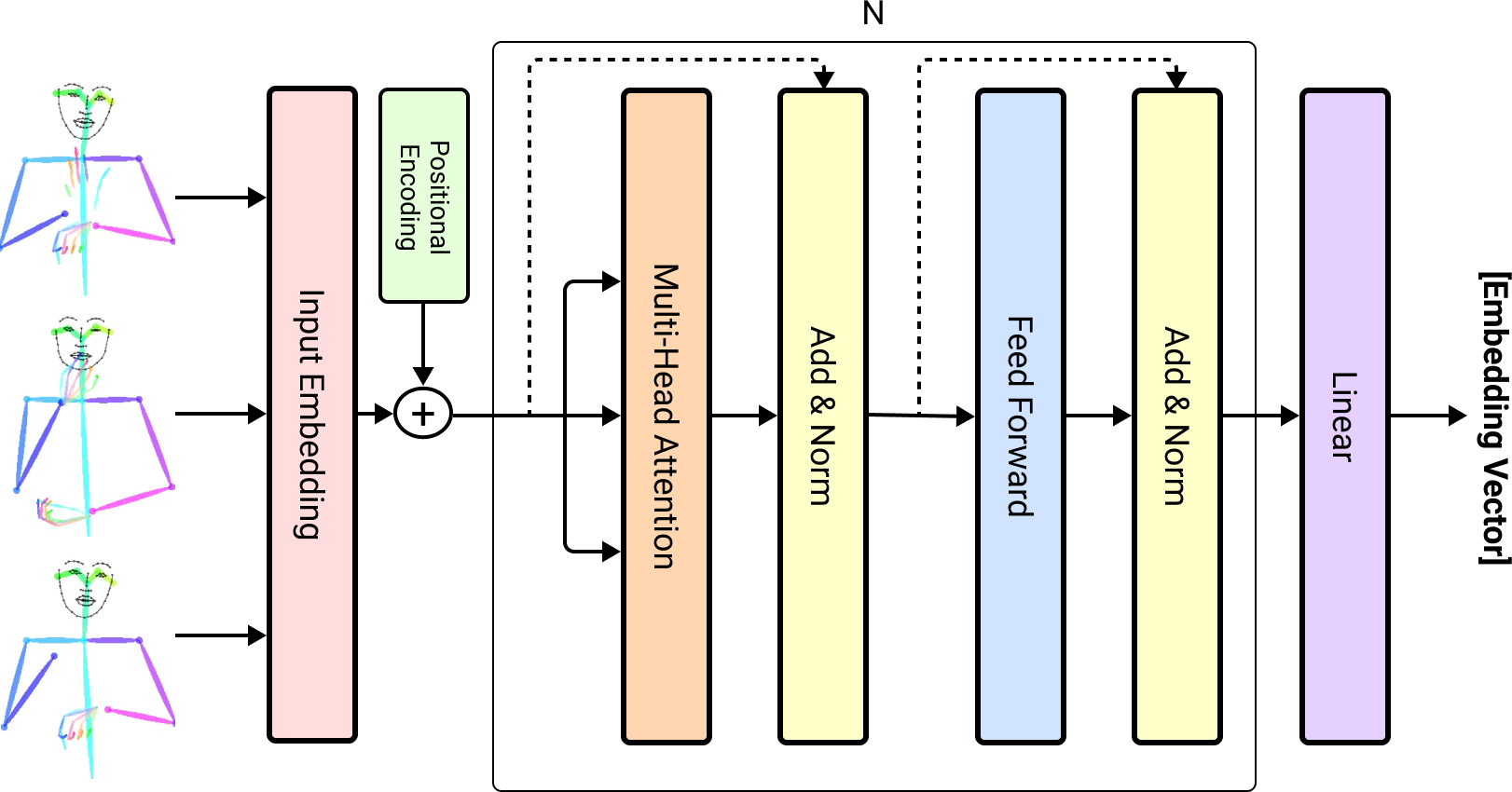
Figure 3: The model receives a sequence of skeleton key-points, creates a vector representation and append information about the sequentiality, and then, the Transformer maps this sequence to an embedding vector.

3.2.1 Pose Embedding

Before passing the input to the Transformer encoder, it is necessary to embed all the sequence $X$ in a $d_{model}$ dimensional space, that corresponds to the Transformer dimension. For this, a feed-forward neural network of one layer and ReLU activation function is used, accordingly to Equation 1.

$$X_{t}^{emb}=\mathrm{ReLU}(\textbf{W}_{e}X_{t}+\textbf{b}_{e})$$ (1)

Where $\textbf{W}_{e}$ and $\textbf{b}_{e}$ are learnable parameters that extracts features from $X_{t}\in\mathbb{R}^{2M}$ and creates a semantic representation $X_{t}^{emb}\in\mathbb{R}^{d_{model}}$ where vectors with a similar context will be closely located in the embedding space.

Nevertheless, one of the properties of the Transformers are the non-recurrence of the input, that permits to pass the entire input sequence in a parallel fashion, as opposite to RNNs. Therefore, to encode the sequentiality of the input sequence, information related to the order of the elements must be introduced to each one of the input embeddings. To accomplish this, a positional encoding vector is added to each input element. This vector is calculated by periodic functions, such as sine and cosine, and it determines the relative distance between input elements by using different frequencies depending on the input element position in the sequence, as shown in Equations 2 and 3.

$$PE_{(pos,2i)} =\sin(pos/1000^{2i/d_{model}})$$ (2)

$$PE_{(pos,2i+1)} =\cos(pos/1000^{2i/d_{model}})$$ (3)

Where $pos$ is the position of the frame in the sequence and $i$ is the embedding space dimension.

3.2.2 Transformer Encoder

The encoder is a stack of $n=2$ layers, where each one contains two sub-layers. The first is a multi-head self-attention mechanism and the second is a fully connected feed-forward network. Around each sub-layer there is a residual connection followed by layer normalization that produces the output of the corresponding sub-layer, as described in Equation 4.

$$\mathrm{Output}=\mathrm{LayerNorm}(x+\mathrm{Sublayer}(x))$$ (4)

Where $\mathrm{Sublayer}$ is the function that the sub-layer implements. Besides, to facilitate the residual connections, all sub-layers will produce outputs with dimension equal to $d_{model}=128$.

3.2.3 Attention

The first sub-layer of the encoder is a self-attention mechanism. It maps a query and key-value pairs to an output, which is computed as the weighted sum of the values, where each weight is computed by a compatibility function with the query and the corresponding key. Each embedding $X_{t}^{emb}$ in the input sequence is multiplied by the learnable parameters matrices $W_{Q}$, $W_{K}$ and $W_{V}$ to produce the matrices $Q$, $K$ and $V$ that corresponds to the packed matrices for the query, key and value, respectively. The output of the attention mechanism is calculated by the Equation 5.

$$\mathrm{Attention}(Q,K,V)=\mathrm{softmax}(\frac{QK^{T}}{\sqrt{d_{k}}})V$$ (5)

Instead of computing only a single attention function, is useful to perform multiple calculations from multiple attention mechanisms in parallel. This allows the model to admit different representations from different sub-spaces. This constitutes the Multi-Head Attention(MHA), and the many outputs are concatenated and projected to get the final MHA results, as described in Equation 6.

$$\mathrm{MultiHead}(Q,K,V)=\mathrm{Concat}(\mathrm{head}_{1},...,\mathrm{head}_{h})W_{O}$$ (6)

Where $\mathrm{head}_{i}$ is the self-attention output for the $i^{th}$ head and $W_{O}$ is the learnable parameter matrix that maps the inputs with dimension $hd_{model}$ to $h_{model}$. The number of heads in this model is set to $h=4$.

3.2.4 Feed-Forward Networks

The second sub-layer in each encoder layer is a fully connected feed-forward network, which applies two linear transformations followed by a ReLU activation to each position separately and identically, as shown in Equation 7.

$$\mathrm{FFN}(x)=\mathrm{max}(0,xW_{1}+b_{1})W_{2}+b2$$ (7)

Where $W_{1}$, $W_{2}$, $b_{1}$ and $b_{2}$ are learnable parameters that differs from layer to layer.

3.3 One-Shot and Few-Shot Classification

Once the embedding vector is obtained from the input video, it lies in a $n$-dimensional space. The mapping from the input video to the embedding vector should be semantic. In other words, given a distance metric, vectors representing inputs of the same class must be closer in space, while vectors of inputs of different classes must be further apart.

The classification step relies on the vector representation of the input videos and the similarities or distances between them. Therefore, the classification consists in taking a few examples of each class and compare the distance of new input vector to each one of them. The example that is closer to the input will define the class of the prediction. Different methods to perform this operation were tested, such as k-Nearest Neighbors, Cosine Similarity and Prototypical Networks. The results will be describe in next sections.

3.3.1 k-Nearest Neighbors

In Machine Learning, k-Nearest Neighbors algorithm (kNN) [39] is a non-parametric algorithm used for classification or regression. In classification, it uses the labeled training data and a distance function, usually Euclidean, to compute the distance between each sample of the set and a given new input. By knowing the label of the training samples, one can define a classification decision rule to predict the input label based on the nearest points. A visual demonstration of kNN can be seen in Figure 4.

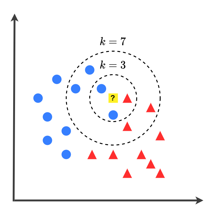
Figure 4: Visualization of k-Nearest Neighbors with two classes (blue circles and red triangles) with $k=3$ and $k=7$.

Consider a training set with $N$ samples where each one of them is a pair $(\textbf{x}_{i},y_{i})$ with $\textbf{x}_{i}=(x_{i}^{1},x_{i}^{2},...,x_{i}^{P})$ being a point with $P$ features and $y_{i}$ being the label of that point. The Euclidean distance between any two points $x_{j}$ and $x_{k}$ is given by the Equation 8:

$$d(\textbf{x}_{j},\textbf{x}_{k})=\sqrt{(x_{j}^{1}-x_{k}^{1})^{2}+(x_{j}^{2}-x_{k}^{2})^{2}+...+(x_{j}^{P}-x_{k}^{P})^{2}}$$ (8)

In kNN algorithm for classification, the variable $k$ represents the number of nearest neighbors used to predict the label of the input based on the $k$ nearest points from the training set. In the case of a 1-nearest neighbor, the class prediction for the input $\textbf{x}_{k}$ will be the class of the nearest training set sample, given by Equation 9.

$$d(\textbf{x}_{i},\textbf{x}_{k})=\min_{i}\{d(\textbf{x}_{i},\textbf{x}_{k})\}$$ (9)

In the case of $k>1$, the predicted class will be the class that appear with most frequency among the $k$ nearest neighbors from the training sample.

3.3.2 Cosine Similarity

The cosine similarity [40] measures how similar are two vectors from a given inner product space. Considering the embedding space Euclidean, the inner product between the vectors A and B can be defined as the sum of the products of the coordinates, as shown in Equation 10:

$$\textbf{A}\cdot\textbf{B}=\sum_{i}^{N}{a_{i}b_{i}}$$ (10)

The inner product can be geometrically interpreted as how aligned the vectors are, as shown in Figure 5. In a way that if they are pointing in the same direction the magnitude will be maximum and if they are perpendicular, the magnitude will be zero. This naturally relates to the cosine of the angle between two vectors. The result can also be normalized by the product of the magnitude of both vectors and the result will vary from -1 to 1. As shown in Equation 11.

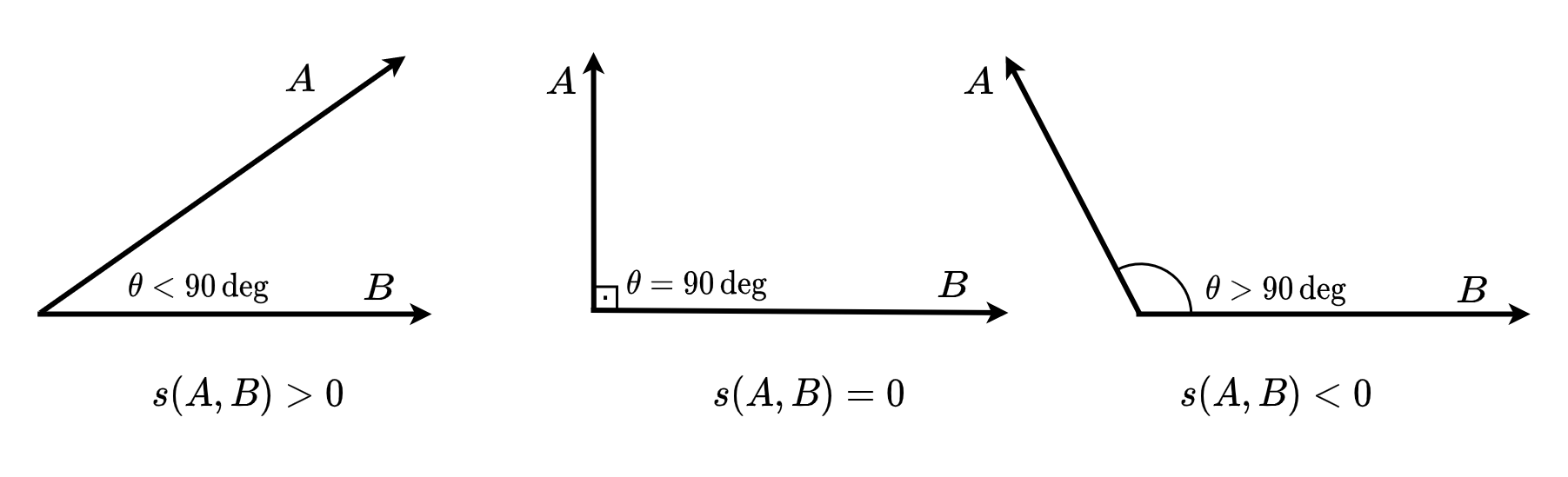
Figure 5: Visualization of Cosine Similarity for $s(\textbf{A},\textbf{B})<0$, $s(\textbf{A},\textbf{B})=0$ and $s(\textbf{A},\textbf{B})>0$ respectively.

$$s(\textbf{A},\textbf{B})=\cos(\theta)=\frac{\textbf{A}\cdot\textbf{B}}{\|\textbf{A}\|\|\textbf{B}\|}$$ (11)

When using cosine similarity as a classifier, the input vector will be compared to all samples of the training set and the predicted class will be the class of the most similar training sample, as shown in Equation 12.

$$s(\textbf{x}_{i},\textbf{x}_{k})=\max_{i}\{s(\textbf{x}_{i},\textbf{x}_{k})\}$$ (12)

3.3.3 Prototypical Networks

Prototypical networks [41], aims to learn a metric space in which classification can be performed by computing distances to prototype representations of each class. It uses an embedding function $f_{\theta}:\mathbb{R}^{D}\to\mathbb{R}^{M}$ with learnable parameters $\theta$ to encode each input into a M-dimensional feature vector $\textbf{c}_{k}\in\mathbb{R}^{M}$. A prototype feature vector is defined as a mean vector of the embedded support points belonging to its class $k$:

$$\textbf{c}_{k}=\frac{1}{|S_{k}|}\sum_{(x_{i},y_{i})\in S_{k}}f_{\theta}(x_{i})$$ (13)

where $S_{k}$ denotes the support set of examples labeled with class $k$.

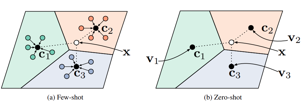
Figure 6: Prototypical networks in the few-shot and zero-shot scenarios. (Source: [41]).

The prototypical networks produce a distribution over classes for a given test input $x$ based on softmax over distances to the prototypes in the embedding space:

$$p_{\theta}(y=k|x)=\frac{exp(-d(f_{\theta}(x),\textbf{c}_{k}))}{\sum_{k^{\prime}}exp(-d(f_{\theta}(x),\textbf{c}_{k}^{\prime}))}$$ (14)

where $d:\mathbb{R}^{M}\times\mathbb{R}^{M}\to[0,+\infty)$ is a differentiable Bregman divergence distance function, for this work, a squared Euclidean distance:

$$\|f_{\theta}(x)-\textbf{c}_{k}\|^{2}$$ (15)

The training process aims to minimize the negative log-probability $\mathcal{J}(\theta)=-logp_{\theta}(y=k|x)$ of the true class $k$ via Stochastic Gradient Descent, Adam, in this case [42].

4 Training

4.1 Data

In this work, we evaluate our method on LSA64 Dataset [43], which is a Argentinian Sign Language dataset. It includes 3200 videos where 10 non-experts subjects perform 5 repetitions of 64 different classes of signs, making 50 videos per sign. The dataset was recorded in two sets. The first was in a outdoors environment, with natural lightning with 23 one-handed signs recorded. The second one was recorded in an indoors environment with artificial lightning and 22 two-handed and 19 one-handed signs were added. The subjects where in a white background, wore black clothes and were standing or sitting while recording. The subjects also wore a fluorescent-colored gloves, to simplify the segmentation process by removing issues with skin color.

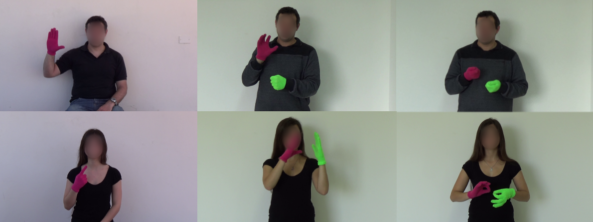
Figure 7: Samples snapshots of LSA64 dataset.

4.2 Triplet Loss

Given an input x, the purpose of the Transformer encoder is to map x to a feature vector representation in the $\mathbb{R}^{d}$ space. It is necessary that these representations encodes the meaning of the input, in this case, the different classes of signs. Good representations for this applications have the characteristics of creating clusters of the same signs even if the input videos are dissimilar. Also, different classes of signs, even if they are recorded by the same person, should be distant in the feature space. To train the Transformer encoder to have this ability, we use Triplet Loss.

Triplet Loss consists of selecting 3 inputs (or points in embedding space), where the reference, or anchor, is compared to a positive points from the same class and a negative points from a different one. The loss function will try to maximize the distance between the anchor and the negative points, while minimizing the distance between the anchor and the positive points. This process will put embedding vectors with the same class closer together and vectors with different classes further apart. An illustration of this process is shown in Figure 8.

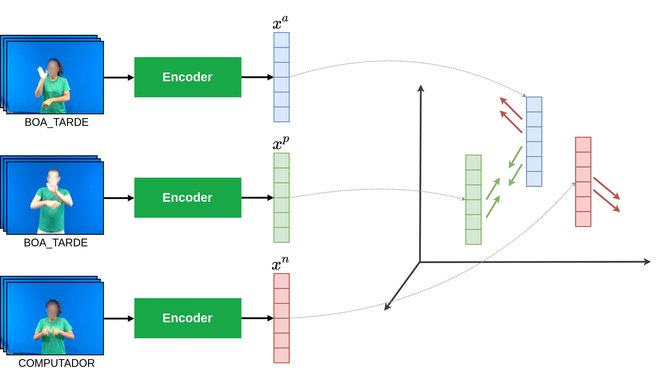
Figure 8: Example of triplet made by a anchor, positive and negative points. Each point is an encoding from the Transformer model. In the training process, the objective is to increase the distance between the anchor and the negative points, while decreasing the distance between the anchor and the positive points.

The loss function $\mathcal{L}(x^{a},x^{p},x^{n})$ will have as inputs embedding vectors representing the anchor point $x^{a}$, the positive point $x^{p}$ and the negative point, $x^{n}$. The loss is calculated to minimize the Euclidean distance between $x^{a}$ and $x^{p}$ and to maximize the distance between $x^{a}$ and $x^{n}$. A margin $\alpha$ is added to the total loss to prevent the model from collapsing all points to the same position, with loss always zero. The Triplet Loss function is calculated accordingly to Equation 16.

$$\mathcal{L}(x^{a},x^{p},x^{n})=\max(\|f(x^{a})-f(x^{p})\|^{2}-\|f(x^{a})-f(x^{n})\|^{2}+\alpha,0)$$ (16)

In this work, a dataset was made by randomly picking 5000 triplets. The process of constructing a triplet consists of randomly choosing two different classes. Two randomly selected non-repeating samples from the first class will serve as anchor and positive points, while a randomly selected sample from the second class will be the negative point. This process will be repeated to construct the training set.

4.3 Implementation Details

The Transformer encoder have the input dimension of 225 elements, which corresponds to the length of the flattened points of skeleton extracted from MediaPipe; The embedding dimension of the model is set to 128; The number of heads of the encoder is 4 with 2 layers and the encoder feed-forward number of units is 1024.

The proposed architecture was implemented and tested in Python programming language in a 64-bit Ubuntu 20.04. The Transformer encoder was implemented using the PyTorch [44] framework and the k-Nearest Neighbors, Cosine Similarity classifiers were implemented with the SciKit Learning [45] library and Propotypical Networks were implemented using learn2learn [46] library. The model training and experiments were conducted on a computer with a Intel Core i7-10750H processor with 2.60GHz, 16 gigabytes of RAM and a NVidia GeForce RTX 2070 with 8 gigabytes of video memory with the libraries CuDNN 8.2.0 and CUDA 11.2.

5 Results

The output of the training phase described in Section 4, the embedding space, can virtually represent any sign that shares some resemblance with the content trained. In this context, few-shot methods can be used to classify unseen signs.

5.1 Few-Shot Classification

The few-shot classification can be performed using different methods that relies on the fact that each input sample can be mapped to a embedding vector, and then, the predicted class will be determined by a given strategy, according to the few samples for each class that will be used as reference. The methods used in this work are Prototypical Networks, k-Nearest Neighbors and Cosine Similarity.

5.1.1 Prototypical Networks

Two main goals was established during the analysis of this method: to check the performance of few-shot classification using Prototypical Networks and to validate, the skeleton interpolation procedure, described in Section 3. To accomplish that first one, we performed the K-Shot N-Way classification protocol in which, is given to the model $N$ classes of signs with $K$ samples each. Each $N$ classes of signs was randomly taken from the 48 signs in training set, each one of them was going to produce a prototype $\textbf{p}_{c}$ which $c\in N$, that each sample was going to be assigned.

During training, we used a support set $S$ and a query set $Q$, both from the training set. The support set $S$ is responsible to produce a cluster prototype and each sample in $Q$ is then assigned to each cluster prototype, then the classification was performed by calculating the Euclidean distance for each cluster prototype, as shown in Equation 15.

The testing phase is similar to training, but with unseen classes, in this way is possible to evaluate the capability of our procedure to produce good clusters representation in order to perform a few-shot classification task.

In that way, we can verify the ability of the model to produce a good feature representation and its capability to classify signs with few samples, as well as few available classes of signs. Our dataset was splitted in two subsets containing 48 signs for training and 16 sings for testing.

The second goal was to validate, the skeleton interpolation procedure, described in section tal. To perform this, we repeated each K-shot N-way experiment twice: with and without the interpolation procedure.

Interpolation?	10-way ACC			8-way ACC
	1-shot	5-shots	10-shots	1-shot	5-shots	10-shots
No	0.500	0.810	0.839	0.625	0.837	0.875
Yes	0.569	0.769	0.849	0.712	0.887	0.875

Table 1: Results obtained with 8 and 10 way classification accuracy.

Interpolation?	6-Ways ACC			4-Ways ACC
	1-shot	5-shots	10-shots	1-shot	5-shots	10-shots
No	0.600	0.850	0.900	0.850	0.875	0.975
Yes	0.683	0.866	0.933	0.824	0.975	0.949

Table 2: Results obtained with 4 and 6 way classification accuracy.

As shown in Table 1 and 2, the Transformer model gets better results as number of shots is increased. It can also be seen that as the number of way increase the model gets worst results, evidencing that the number of clusters has influence in the performance accuracy, in other words, the worst scenario is when the number of way is at its maximum.

It can also be noted that the experiments with interpolation procedure outperformed its counterparts in almost every scenarios, and because of that, the interpolation as a pre-processing step was adopted in the subsequent experiments.

5.1.2 k-Nearest Neighbors

In order to test the k-Nearest Neighbors algorithm in the classification task, it is necessary to determine a value for $k$ which is the number of nearest neighbors used to make the prediction. The choice of setting $n=k$ instead of fixing the value of $n$ and varying only $k$ is to simulate real world scenarios where there is little available data, making it necessary to use the maximum of available information. The number of test samples for each class is set equal to $k$, varying from 1 to 8. The number of signs used for training is also evaluated from 10 to 45 in increments of 5.

For this experiment, the test set containing 16 classes never seen in training was used. The accuracy of each combination of $k=n$ with the number of training classes was evaluated 40 times. The Table 3 shows the mean accuracy for each experiment.

# train signs	$k=1$	$k=2$	$k=3$	$k=4$	$k=5$	$k=6$	$k=7$	$k=8$
10	0.651	0.622	0.709	0.732	0.743	0.754	0.770	0.771
15	0.651	0.640	0.725	0.752	0.763	0.775	0.780	0.788
20	0.673	0.643	0.740	0.739	0.771	0.771	0.779	0.790
25	0.681	0.654	0.739	0.759	0.767	0.781	0.788	0.798
30	0.654	0.630	0.704	0.722	0.740	0.752	0.764	0.764
35	0.637	0.632	0.693	0.729	0.738	0.761	0.764	0.769
40	0.684	0.652	0.745	0.754	0.779	0.787	0.796	0.801
45	0.704	0.674	0.767	0.782	0.794	0.807	0.816	0.821

Table 3: Results of kNN for classification varying the number of signs used for training the Transformer encoder, and keeping the number of test samples from each class equal to $k$, from $1$ to $8$.

As the results shows, increasing the number of training classes have a positive effect on the accuracy, even if the number of triplets in the training set is the same. Increasing $k$ also have a positive effect, since more points in feature space are used as reference. Despite the fact that the accuracy tend to increase with the train signs and $k$, some random fluctuations are observed because the size of the training and testing set as well as the randomness of the experiment. Additionally, the confusion matrix of the combination of maximum accuracy, with $k=n=8$ and the number of training signs is 45, is shown in Figure 9.

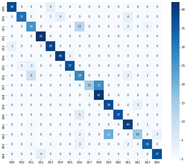
Figure 9: Confusion matrix for kNN used in classification task with $k=8$ with model trained with 45 signs.

The main diagonal of the confusion matrix is where the values are higher. This occurs when the predictions are correct. Besides, it can also be noticed that some positions other than the main diagonal are non-zero. These bad predictions happens when the model convert signs from different classes that share some level of semantic information. This causes the classification algorithms to mislabel these samples. For example, the sign 057 corresponds to "dance" while the sign 058 corresponds to "bathe". Those signals have similar gestures, as shown in Figure 10.

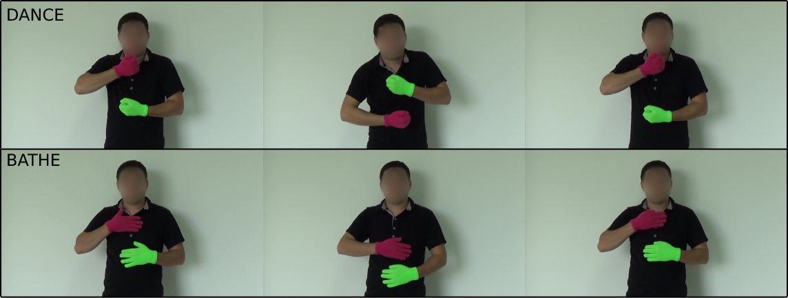
Figure 10: Comparison between the signs of "dance" and "bathe". In some samples the model mislabeled these signs because of their gesture similarity.

5.1.3 Cosine Similarity

The experiments of cosine similarity in classification task had the same configuration of the kNN experiment. The number of training classes varies from 10 to 45 in steps of 5. The number of test samples for each class, $n$, varies from 1 to 8 with classes never seen in training. For classification using cosine similarity, only the most similar sample from the test set is used to make the class prediction. In other words, the similarity between the input with all test samples are calculated and the most similar sample will determine the predicted class. The accuracy of each experiment combination was evaluated 40 times. The Table 4 shows the mean accuracy of the experiments.

# train signs	$n=1$	$n=2$	$n=3$	$n=4$	$n=5$	$n=6$	$n=7$	$n=8$
10	0.651	0.719	0.769	0.803	0.817	0.834	0.850	0.854
15	0.651	0.745	0.779	0.812	0.825	0.841	0.855	0.865
20	0.673	0.744	0.788	0.815	0.834	0.850	0.861	0.875
25	0.681	0.747	0.784	0.805	0.822	0.836	0.850	0.862
30	0.654	0.728	0.751	0.782	0.804	0.823	0.831	0.842
35	0.637	0.717	0.755	0.790	0.809	0.834	0.843	0.855
40	0.684	0.752	0.796	0.821	0.836	0.853	0.860	0.872
45	0.704	0.771	0.815	0.834	0.853	0.870	0.880	0.890

Table 4: Results of cosine similarity for classification varying the number of signs used for training the Transformer encoder and the number of samples from each test class, $n$, from $1$ to $8$.

The results show a positive correlation between the number of training signs, as well as the number of samples for each test class, $n$, with the accuracy. For this model, the results with cosine similarity were better than the ones with kNN. The maximum accuracy occurs when the number of training signs is at maximum, 45, and the number of test samples per class is also at maximum, $n=8$. This best combination was used to generate a confusion matrix for the test set, as shown in Figure 11.

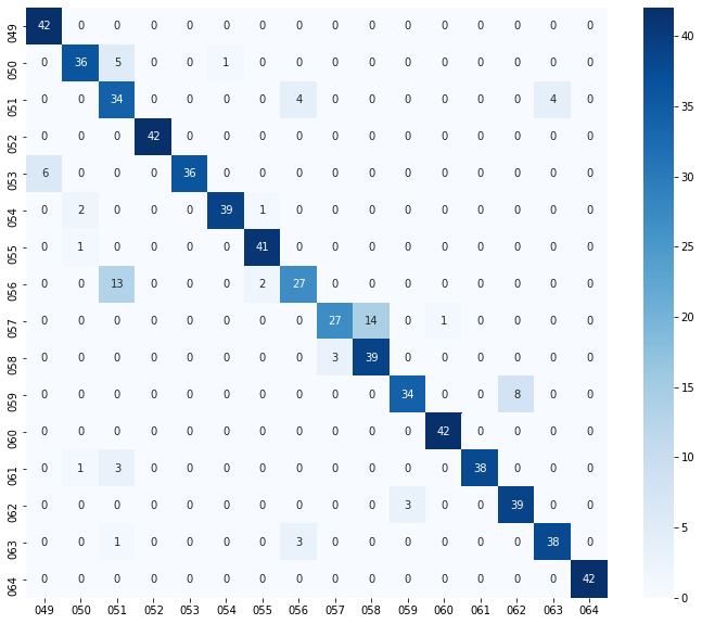
Figure 11: Confusion matrix for cosine similarity used in classification task with $n=8$ with model trained with 45 signs.

As in the kNN tests, the confusion matrix for cosine similarity also have most signs labeled correctly, as the main diagonal suggests, with less mislabeling. Still, a small quantity of signs are classified incorrectly for the same reasons as kNN.

5.2 Visualizing the Embedding Vector Space

It is infeasible to visualize the high-dimensional feature space produced by the Transformer model. Then, in order to gain a notion of the distribution of the embedding space, we make use of the dimensionality reduction technique t-SNE (t-Distributed Stochastic Neighbor Embedding)[47].

t-SNE converts affinities of data points to probabilities. The affinities in the original space are represented by Gaussian joint probabilities and the affinities in the embedded space are represented by Student’s t-distributions. This allows t-SNE to be particularly sensitive to local structure, that structure can be seen at many scales on a single map.

In this work, the visualizations of the embedding vector space were produced by t-SNE, which can be considered a manifold approach to dimensionality reduction. In the Figure 12 the embedding vectors for the training samples can be seen in two dimensions. Each color represents a class and each point represents a training sample.

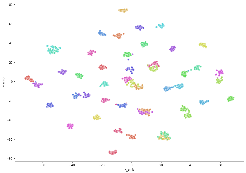
Figure 12: Visualization of training data in embedding space with reduced dimensionality using t-SNE. Each color represents a class and each point represents a sample.

As the low-dimensional representation of the training signs suggests, the model could organize different classes into clusters, with a certain distance between the clusters. Although, there still a few signs that are similar which make them closer in the embedding space.

The same experiment were conducted for 16 signs classes, with 50 samples per class, from the test set that were never seen in the training, as shown in Figure 13.

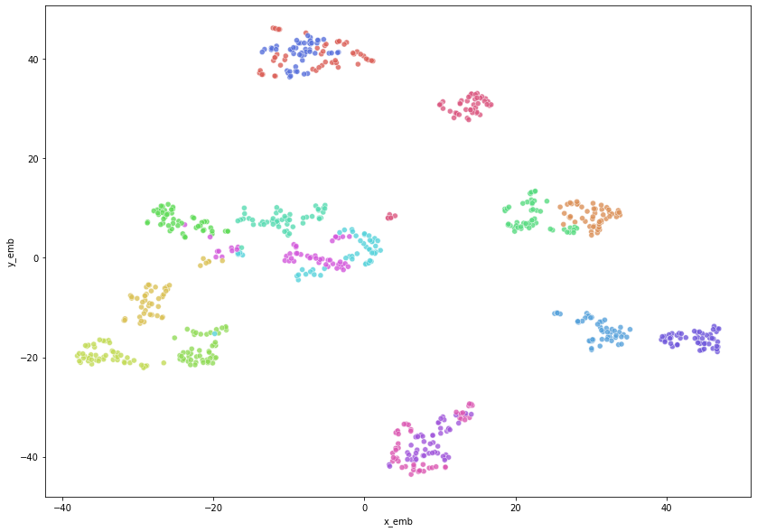
Figure 13: Visualization of test data in embedding space with reduced dimensionality using t-SNE. Each color represents a class and each point represents a sample.

As seen in the plot, the model could form clusters for signs never seen in the training, suggesting that the model achieved the ability for grouping new similar signs while keeping different ones distant in the embedding space.

6 Conclusions

We have demonstrated that a Transformer encoder model can generate useful representations of sequences of body keypoints by a contrastive learning training approach. The model eventually learned to extract useful features from the input sequence in a parallel way without losing temporal information, considering the positional encoding. This hypothesis was tested and validated by performing a classification task using kNN, cosine similarity and prototypical networks that achieved accuracies close to 90%. The positive correlation of the accuracy with the number of training signs suggests that a large variety of classes is beneficial for the model, even with a small number of samples per class, in this case, 50. The majority of classification results for kNN and cosine similarity being in the main diagonal of the confusion matrices, indicates that the model not only had a high accuracy, but also could classify correctly most of the samples. The mislabels occurred with signs from classes that are similar in how they are gesticulated, which put them closer in the embedding space. Furthermore, the visualization of the embedding space using dimensionality reduction, such as t-SNE, for predictions of samples never seen in the training suggests that the model achieved a good capacity of clustering similar video signs, while making the different ones more distant in the feature space.

As future works, datasets with a larger variety of classes can be constructed, including different languages. The expressiveness and interpretability of the Transformer can also be analyzed through visualization of the internal attention weights.

References

- [1] Kanchon Kanti Podder, Muhammad EH Chowdhury, Anas M Tahir, Zaid Bin Mahbub, Amith Khandakar, Md Shafayet Hossain, and Muhammad Abdul Kadir. Bangla sign language (bdsl) alphabets and numerals classification using a deep learning model. Sensors, 22(2):574, 2022.
- [2] World Health Organization et al. World report on hearing. 2021.
- [3] Ronice Müller de Quadros. Linguistic policies, linguistic planning, and brazilian sign language in brazil. Sign Language Studies, 12(4):543–564, 2012.
- [4] Michael A Schwartz, Brent C Elder, Monu Chhetri, and Zenna Preli. Falling through the cracks: Deaf new americans and their unsupported educational needs. Education Sciences, 12(1):35, 2022.
- [5] Jorge Daniel Barros Junior. Tradução automática de línguas de sinais: do sinal para a escrita. 2016.
- [6] Emely Pujólli da Silva and Paula Dornhofer Paro Costa. Qlibras: A novel database for grammatical facial expressions in brazilian sign language. In Proceeding of the X Meeting of Students and Teachers of DCA/FEEC/UNICAMP (EADCA), 2017.
- [7] Jampierre Rocha, Jeniffer Lensk, Taís Ferreira, and Marcelo Ferreira. Towards a tool to translate brazilian sign language (libras) to brazilian portuguese and improve communication with deaf. In 2020 IEEE Symposium on Visual Languages and Human-Centric Computing (VL/HCC), pages 1–4. IEEE, 2020.
- [8] Dongxu Li, Cristian Rodriguez, Xin Yu, and Hongdong Li. Word-level deep sign language recognition from video: A new large-scale dataset and methods comparison. In Proceedings of the IEEE/CVF winter conference on applications of computer vision, pages 1459–1469, 2020.
- [9] Helen Cooper, Brian Holt, and Richard Bowden. Sign language recognition. In Visual analysis of humans, pages 539–562. Springer, 2011.
- [10] Kouichi Murakami and Hitomi Taguchi. Gesture recognition using recurrent neural networks. In Proceedings of the SIGCHI conference on Human factors in computing systems, pages 237–242, 1991.
- [11] Jong-Sung Kim, Won Jang, and Zeungnam Bien. A dynamic gesture recognition system for the korean sign language (ksl). IEEE Transactions on Systems, Man, and Cybernetics, Part B (Cybernetics), 26(2):354–359, 1996.
- [12] Chan-Su Lee, Zeungnam Bien, Gyu-Tae Park, Won Jang, Jong-Sung Kim, and Sung-Kwon Kim. Real-time recognition system of korean sign language based on elementary components. In Proceedings of 6th International Fuzzy Systems Conference, volume 3, pages 1463–1468. IEEE, 1997.
- [13] Manjula B Waldron and Soowon Kim. Isolated asl sign recognition system for deaf persons. IEEE Transactions on rehabilitation engineering, 3(3):261–271, 1995.
- [14] Ming-Hsuan Yang, Narendra Ahuja, and Mark Tabb. Extraction of 2d motion trajectories and its application to hand gesture recognition. IEEE Transactions on pattern analysis and machine intelligence, 24(8):1061–1074, 2002.
- [15] Thad Starner and Alex Pentland. Real-time american sign language recognition from video using hidden markov models. In Motion-based recognition, pages 227–243. Springer, 1997.
- [16] Kirsti Grobel and Marcell Assan. Isolated sign language recognition using hidden markov models. In 1997 IEEE International Conference on Systems, Man, and Cybernetics. Computational Cybernetics and Simulation, volume 1, pages 162–167. IEEE, 1997.
- [17] Jung-Bae Kim, Kwang-Hyun Park, Won-Chul Bang, Jong-Sung Kim, et al. Continuous korean sign language recognition using automata-based gesture segmentation and hidden markov model. Control Robot Systems Society: Proceedings of the Conference, pages 105–2, 2001.
- [18] Mohammed Waleed Kadous et al. Machine recognition of auslan signs using powergloves: Towards large-lexicon recognition of sign language. In Proceedings of the Workshop on the Integration of Gesture in Language and Speech, volume 165, 1996.
- [19] Lionel Pigou, Sander Dieleman, Pieter-Jan Kindermans, and Benjamin Schrauwen. Sign language recognition using convolutional neural networks. In European Conference on Computer Vision, pages 572–578. Springer, 2014.
- [20] Hueihan Jhuang, Thomas Serre, Lior Wolf, and Tomaso Poggio. A biologically inspired system for action recognition. In 2007 IEEE 11th international conference on computer vision, pages 1–8. Ieee, 2007.
- [21] Jie Huang, Wengang Zhou, Houqiang Li, and Weiping Li. Sign language recognition using 3d convolutional neural networks. In 2015 IEEE international conference on multimedia and expo (ICME), pages 1–6. IEEE, 2015.
- [22] Zhen Zuo, Bing Shuai, Gang Wang, Xiao Liu, Xingxing Wang, Bing Wang, and Yushi Chen. Convolutional recurrent neural networks: Learning spatial dependencies for image representation. In Proceedings of the IEEE conference on computer vision and pattern recognition workshops, pages 18–26, 2015.
- [23] Kshitij Bantupalli and Ying Xie. American sign language recognition using deep learning and computer vision. In 2018 IEEE International Conference on Big Data (Big Data), pages 4896–4899. IEEE, 2018.
- [24] Ashish Vaswani, Noam Shazeer, Niki Parmar, Jakob Uszkoreit, Llion Jones, Aidan N Gomez, Łukasz Kaiser, and Illia Polosukhin. Attention is all you need. In Advances in neural information processing systems, pages 5998–6008, 2017.
- [25] Jacob Devlin, Ming-Wei Chang, Kenton Lee, and Kristina Toutanova. Bert: Pre-training of deep bidirectional transformers for language understanding. arXiv preprint arXiv:1810.04805, 2018.
- [26] Rohit Girdhar, Joao Carreira, Carl Doersch, and Andrew Zisserman. Video action transformer network. In Proceedings of the IEEE/CVF Conference on Computer Vision and Pattern Recognition, pages 244–253, 2019.
- [27] Necati Cihan Camgoz, Oscar Koller, Simon Hadfield, and Richard Bowden. Sign language transformers: Joint end-to-end sign language recognition and translation. In Proceedings of the IEEE/CVF conference on computer vision and pattern recognition, pages 10023–10033, 2020.
- [28] Tao Jiang, Necati Cihan Camgoz, and Richard Bowden. Skeletor: Skeletal transformers for robust body-pose estimation. In Proceedings of the IEEE/CVF Conference on Computer Vision and Pattern Recognition, pages 3394–3402, 2021.
- [29] Grigorii Shovkoplias, Mark Tkachenko, Arip Asadulaev, Olga Alekseeva, Natalia Dobrenko, Daniil Kazantsev, Alexandra Vatian, Anatoly Shalyto, and Natalia Gusarova. Support for communication with deaf and dumb patients via few-shot machine learning.
- [30] Yunus Can Bilge, Ramazan Gokberk Cinbis, and Nazli Ikizler-Cinbis. Towards zero-shot sign language recognition. IEEE Transactions on Pattern Analysis and Machine Intelligence, 2022.
- [31] Florian Schroff, Dmitry Kalenichenko, and James Philbin. Facenet: A unified embedding for face recognition and clustering. In Proceedings of the IEEE conference on computer vision and pattern recognition, pages 815–823, 2015.
- [32] Keiron O’Shea and Ryan Nash. An introduction to convolutional neural networks. arXiv preprint arXiv:1511.08458, 2015.
- [33] Alexey Dosovitskiy, Lucas Beyer, Alexander Kolesnikov, Dirk Weissenborn, Xiaohua Zhai, Thomas Unterthiner, Mostafa Dehghani, Matthias Minderer, Georg Heigold, Sylvain Gelly, et al. An image is worth 16x16 words: Transformers for image recognition at scale. arXiv preprint arXiv:2010.11929, 2020.
- [34] Yoshua Bengio, Aaron Courville, and Pascal Vincent. Representation learning: A review and new perspectives. IEEE transactions on pattern analysis and machine intelligence, 35(8):1798–1828, 2013.
- [35] Ian Goodfellow, Yoshua Bengio, and Aaron Courville. Deep learning. MIT press, 2016.
- [36] Zhe Cao, Gines Hidalgo, Tomas Simon, Shih-En Wei, and Yaser Sheikh. Openpose: realtime multi-person 2d pose estimation using part affinity fields. IEEE transactions on pattern analysis and machine intelligence, 43(1):172–186, 2019.
- [37] Camillo Lugaresi, Jiuqiang Tang, Hadon Nash, Chris McClanahan, Esha Uboweja, Michael Hays, Fan Zhang, Chuo-Ling Chang, Ming Guang Yong, Juhyun Lee, et al. Mediapipe: A framework for building perception pipelines. arXiv preprint arXiv:1906.08172, 2019.
-
[38]
Google LLC.
Holistic. imagem, fig 2. mediapipe holistic pipeline overview.
feb 2020.
Available online:
https://google.github.io/mediapi
pe/solutions/holistic.html (accessed on 10 Fabruary 2022). - [39] Oliver Kramer. K-nearest neighbors. In Dimensionality reduction with unsupervised nearest neighbors, pages 13–23. Springer, 2013.
- [40] Najim Dehak, Reda Dehak, James R Glass, Douglas A Reynolds, Patrick Kenny, et al. Cosine similarity scoring without score normalization techniques. In Odyssey, page 15, 2010.
- [41] Jake Snell, Kevin Swersky, and Richard Zemel. Prototypical networks for few-shot learning. In Proceedings of the 31st International Conference on Neural Information Processing Systems, pages 4080–4090, 2017.
- [42] Diederik P Kingma and Jimmy Ba. Adam: A method for stochastic optimization. arXiv preprint arXiv:1412.6980, 2014.
- [43] Franco Ronchetti, Facundo Quiroga, Cesar Estrebou, Laura Lanzarini, and Alejandro Rosete. Lsa64: A dataset of argentinian sign language. XX II Congreso Argentino de Ciencias de la Computación (CACIC), 2016.
- [44] Nikhil Ketkar and Jojo Moolayil. Introduction to pytorch. In Deep learning with python, pages 27–91. Springer, 2021.
- [45] Gavin Hackeling. Mastering Machine Learning with scikit-learn. Packt Publishing Ltd, 2017.
- [46] Sébastien M. R. Arnold, Praateek Mahajan, Debajyoti Datta, Ian Bunner, and Konstantinos Saitas Zarkias. learn2learn: A library for meta-learning research, 2020.
- [47] Laurens Van der Maaten and Geoffrey Hinton. Visualizing data using t-sne. Journal of machine learning research, 9(11):2579–2605, 2008.