Scaling theory for the statistics of slip at frictional interfaces

Abstract

Slip at a frictional interface occurs via intermittent events. Understanding how these events are nucleated, can propagate, or stop spontaneously remains a challenge, central to earthquake science and tribology. In the absence of disorder, rate-and-state approaches predict a diverging nucleation length at some stress $\sigma^{*}$, beyond which cracks can propagate. Here we argue for a flat interface that disorder is a relevant perturbation to this description. We justify why the distribution of slip contains two parts: a powerlaw corresponding to ‘avalanches’, and a ‘narrow’ distribution of system-spanning ‘fracture’ events. We derive novel scaling relations for avalanches, including a relation between the stress drop and the spatial extension of a slip event. We compute the cut-off length beyond which avalanches cannot be stopped by disorder, leading to a system-spanning fracture, and successfully test these predictions in a minimal model of frictional interfaces.

1 Introduction

When a frictional interface is driven quasistatically, periods of loading are punctuated by sudden macroscopic slip events. Field observations on earthquakes Rice (1993); Scholz (1998) and laboratory studies support that slip nucleates at weak regions of the interface and then propagates ballistically as a fracture Xia et al. (2004); Rubinstein et al. (2004); Ben-David et al. (2010); Passelègue et al. (2013); Heaton (1990); Zheng and Rice (1998); Roch et al. (2022); Svetlizky and Fineberg (2014); Svetlizky et al. (2016). Understanding under which conditions large slip events are triggered and can propagate is central to tribology, for example to explain the observed variability of friction coefficients Ben-David and Fineberg (2011); Popov (2010); Rabinowicz (1992). It is also key for earthquake science Brace and Byerlee (1966). Earthquakes are powerlaw distributed when averaged over many faults Gutenberg and Richter (1954). When fault specific data are considered, observations are debated. Some studies find a bimodal distribution, consisting of a powerlaw behaviour at small magnitude on several decades, an absence of events at intermediate magnitude, and a few top outliers for which the magnitude is large Wesnousky (1994). Other studies suggest instead a continuous powerlaw Page et al. (2011). This debate is complicated by the fact that an individual fault consists of many segments, whose length distribution is itself self-similar Manighetti et al. (2009). Here we propose an explanation for the bimodal distribution of slip events when slip occurs at a single interface, which we consider to be disordered but essentially flat.

These questions are complicated by the fact that frictional forces can decrease with sliding velocity. Various mechanisms can lead to such a velocity-weakening, including thermal creep Scholz and Engelder (1976); Baumberger and Caroli (2006); Rabinowicz (1956); Marone (1998); Heslot et al. (1994); Vincent-Dospital et al. (2020) or the mere effect of inertia Fisher et al. (1997); Ramanathan et al. (1997); Schwarz and Fisher (2001); Salerno et al. (2012). Rate-and-state models Dieterich (1979); Rice and Ruina (1983); Ruina (1983); Scholz (1998) describe the dynamics of frictional interfaces via differential equations that capture velocity weakening. The latter is characterised by a length scale $L_{c}$ below which its effect is small in comparison to elastic forces Lebihain et al. (2021); Perfettini et al. (2003); Ray and Viesca (2017); Dublanchet (2018); Albertini et al. (2021); Schär et al. (2021). Importantly, in the case where the stress as a function sliding velocity displays a minimum $\sigma_{\min}$, this approach predicts Zheng and Rice (1998); Ohnaka and Kuwahara (1990); Brener et al. (2018) a characteristic stress $\sigma^{*}$ very close to $\sigma_{\min}$, beyond which a slip pulse of spatial extension larger than $L^{*}$ will invade the system. In Brener et al. (2018), it is found that $L^{*}/L_{c}\sim(\sigma-\sigma^{*})^{-1}$. Yet, these results apply when the interface is homogeneous: their validity in the presence of disorder nor their connection to the observed broad distribution of earthquakes is clear.

Another approach describes how an elastic manifold driven through a disordered medium can be pinned by disorder Fisher (1983, 1998), and was specifically applied to frictional interfaces Fisher (1983); Fisher et al. (1997); Fisher (1998); Ramanathan et al. (1997). In simple settings that exclude the existence of velocity weakening, the stress of a quasistatically driven interface converges to some critical value, where slip events are powerlaw distributed. Unfortunately, these results do not apply in presence of velocity-weakening effects where even the presence of large avalanches was debated Fisher et al. (1997); Dahmen et al. (1998); Schwarz and Fisher (2003); Maimon and Schwarz (2004) , yet experimentally observed in Baldassarri et al. (2006). Very recently de Geus et al. (2019), we introduced a minimal model of frictional interfaces that contains long-range elastic interactions, disorder, and inertia. Criticality was observed, with powerlaw avalanches whose size can span four decades as the stress reaches some critical value $\sigma_{c}$. Yet, inertia introduces novel phenomena. For example, in a finite system the distribution of events is bimodal: powerlaw distributed avalanches co-exist with system-spanning events. Which mechanism causes such large avalanches, and how their duration, length scale, and stress drop are related to each other remain unknown. So is the relationship between $\sigma_{c}$ governing avalanches and rate-and-state approaches.

In this article, we argue theoretically that $\sigma_{c}=\sigma^{*}$, implying that rate-and-state approaches capture the critical stress affecting the slip statistics. Yet, we find that disorder is a relevant perturbation: consequently, previous results for the diverging nucleation length scale near $\sigma_{c}$ neither based on a homogeneous system Brener et al. (2018) nor on Griffith’s argument de Geus et al. (2019) apply. Our current analysis justifies the presence of large powerlaw avalanches and leads to scaling relations between their length, stress drop, and duration; which are found to be related to a fractal property of the slip geometry at the interface. We successfully test all predictions numerically in the minimal model of de Geus et al. (2019).

2 Scaling theory for slip events with velocity weakening

Observables describing slip events

We characterise slip events by their linear spatial extension (or ‘width’ in one dimension) $A$, the total slip (the increment of slip, or increment of displacement discontinuity, integrated across the event’s ‘width’) $S$, and their duration $T$. As sketched in Fig. 1A and as reported in some systems displaying stick-slip Wesnousky (1994); Schwarz and Fisher (2001); de Geus et al. (2019), the distribution $P(S)$ consists of two parts. First, there is a powerlaw distribution cut-off beyond some characteristic value $S_{c}$, i.e. $P_{a}(S)=S^{-\tau}f(S/S_{c})$ where $f$ is a rapidly decreasing function of its argument. We call the associated events ($S<S_{c}$) ‘avalanches’ and denote by $A_{c}$ their cut-off spatial extension along the interface. Second, there are system-spanning slip events of extension $A\approx L$, where $L$ is the system size, resulting in the ‘bump’ at large $S$ in Fig. 1A. Empirical observations Gutenberg and Richter (1944); Kagan (2014) support the existence of scaling behaviours for avalanches:

$$P(S) \sim S^{-\tau},$$ (1)

$$S \sim A^{d_{f}},$$ (2)

$$T \sim A^{z}.$$ (3)

A fourth scaling relation was instead observed in the simple model of interface of de Geus et al. (2019):

$$A_{c}\sim(\sigma-\sigma_{c})^{-\nu}.$$ (4)

(A)

(B)

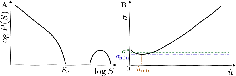
Figure 1: LABEL:sub@fig:theory:PS. Sketch of distribution of avalanche sizes in a finite system: on the left there is a powerlaw distribution cut-off beyond some characteristic value $S_{c}$, on the right there are system-spanning events. LABEL:sub@fig:theory:flow. Sketch of a flow curve (stress $\sigma$ vs slip rate $\dot{u}$) with a minimum at $\sigma=\sigma_{\min}$. (with corresponding slip rate $\dot{u}_{\min}$).

Observables describing the static interface

We consider an interface that is overall flat and homogeneously loaded. Disorder can be exogenous, stemming for example from asperities on the surfaces of the two bodies, or instead be endogenous and result from the history from previous slip events that lead to irregular stresses along the interface. Upon loading, the interface will acquire some slip $u(r)$ at location $r$. Due to the disorder, $u(r)$ will fluctuate spatially. These fluctuations can be characterised by introducing the roughness exponent $\zeta$ of the interface Fisher (1998):

$$||u(r)-u(r^{\prime})||\sim||r-r^{\prime}||^{\zeta}$$ (5)

with $||\ldots||$ the root-mean-square.

We have so far introduced five exponents: $\tau$, $\zeta$, $\nu$, $z$, $d_{f}$. Our central goal is to propose three new scaling relations relating $\zeta$, $\nu$, $z$, $d_{f}$ together, allowing for a stringent empirical test of our views.

Effect of disorder on the rate-and-state description

Previous attempts to describe the joint effects of disorder and velocity-weakening sought to treat the latter as a perturbation Fisher et al. (1997); Dahmen et al. (1998). We take the opposite approach, and seek to characterise how disorder affects the dynamics of a homogeneous interface subjected to velocity weakening, as captured by the rate-and-state description Zheng and Rice (1998); Brener et al. (2018). The relationship $\sigma(\dot{u})$ between the far-field stress $\sigma$ and the slip rate $\dot{u}$, at any location, is key in this approach. If it does display a minimum $\sigma_{\min}$ for some slip rate $\dot{u}_{\min}$ as illustrated in Fig. 1B, then it was shown that beyond some stress $\sigma^{*}$ just above $\sigma_{\min}$, slip events of length $L^{*}\sim(\sigma-\sigma^{*})^{-1}$ can nucleate system-spanning events Brener et al. (2018).

However, where it makes sense for a homogeneous system to consider $\sigma^{*}$ as a quantity that does not vary in space, in a disordered system its structure is locally random. A patch of material of linear extension $A$ can still be described by some effective threshold $\sigma^{*}(A)$, but this quantity must vary in space. $\sigma^{*}(A)$ thus display fluctuations, whose magnitude we denote $\delta\sigma^{*}(A)$. They can only disappear in the thermodynamic limit $A\rightarrow\infty$ where randomness self-averages and homogenisation is achieved. In general one expects:

$$\delta\sigma^{*}\sim A^{-\chi}.$$ (6)

Classical arguments based on disorder imply $\chi\leq(d+\zeta)/2$ Chayes et al. (1986); Fisher (1998) . Here, $d$ is the dimension of the interface (separating objects of dimensions $d+1$). Below, we will provide data supporting that this bound is not saturated.

If $\chi\leq 1$ (as we shall confirm empirically for $d=1$), we now argue that due to these fluctuations, rate-and-state results on nucleation in homogeneous systems cannot apply to disordered ones. Indeed, consider $\sigma-\sigma^{*}$ to be small but positive, and a slip event occurring on a length scale $L^{*}\sim(\sigma-\sigma^{*})^{-1}$. On that length scale, the fluctuations of $\sigma^{*}$ are stronger than the distance to threshold $\sigma-\sigma^{*}$ when the latter is small: $\delta\sigma^{*}(L^{*})\sim(L^{*})^{-\chi}\sim(\sigma-\sigma^{*})^{\chi}\geq(\sigma-\sigma^{*})$. Thus this theory neglecting the fluctuations of $\sigma^{*}$ cannot self-consistently hold near threshold.

Roughness of the interface

As discussed above, the strength $\sigma^{*}(A)$ of a patch of size $A$ varies in space. The interface must adjust to these variations: the slip $u(r)$ will be larger at locations $r$ where $\sigma^{*}(A)$ is small. Fluctuations of elastic stresses follow fluctuations of strain, which between two points $r$ and $r^{\prime}$ are of order ${||u(r)-u(r^{\prime})||/||r-r^{\prime}||}$. If $||r-r^{\prime}||\sim A$, using Eq. 5 these fluctuations are of order $A^{\zeta-1}$. As is more generally the case for an elastic manifold in disordered environments Fisher (1998), we expect such adjustments of the interface slip to stop when these fluctuations of elastic stresses are of order of the fluctuations of $\sigma^{*}(A)$ on that scale (of order $A^{-\chi}$, see Eq. 6), leading to:

$$\chi=1-\zeta.$$ (7)

Justifying powerlaw avalanches

We now argue that Eq. 6 gives a natural explanation for the presence of powerlaw slip events or ‘avalanches’. Consider a system at $\sigma=\sigma^{*}$ where a slip starts to occur at the origin, whose extension grows in time as $A(t)$. During this process, the system encounters new realisations of the disorder, and also explores larger regions of space. Thus, the effective threshold $\sigma^{*}(A(t))$ for slip propagation felt on that scale will vary in time. The dynamics will stop if it becomes larger than the applied stress, i.e. ${\sigma^{*}(A(t))>\sigma^{*}=\sigma}$.

Following the depinning literature, simple arguments then constrain the statistics of stopping events Fisher (1998). $\sigma^{*}(A(t))$ can be thought as a random variable that evolves continuously around its mean $\sigma^{*}$. $\sigma^{*}(A(t))$ will lose memory of its current value when the patch size $A(t)$ increases significantly, i.e. $\sigma^{*}(A(t_{1}))$ at time $t_{1}>t_{0}$ decorrelates from $\sigma^{*}(A(t_{0}))$ when $A(t_{1})-A(t_{0})\geq A(t_{0})$. As a result, every time $A$ doubles in size, there is a finite probability $p_{2}$ that $\sigma^{*}(A(t))-\sigma^{*}$ has changed sign, and that slip has stopped. Such a property implies a powerlaw distribution $P(A)\sim A^{-\tau_{A}}$ with $\tau_{A}=1-\ln(1-p_{2})/\ln(2)$ . Thus we predict that the stress $\sigma_{c}$ at which avalanches are powerlaw, follows:

$$\sigma_{c}=\sigma^{*}.$$ (8)

Maximal avalanche extension $A_{c}$

Consider the same argument applied to the case $\sigma>\sigma^{*}$. As long as the scale of fluctuations $\delta\sigma^{*}(A)\gg\sigma-\sigma^{*}$, the difference $\sigma-\sigma^{*}$ is insignificant (as sketched in Fig. 2), and one recovers a powerlaw distribution of slip events as argued above. However, in the other limit where $\delta\sigma^{*}(A)\ll\sigma-\sigma^{*}$, one always has $\sigma^{*}(A)<\sigma$. In that regime, disorder cannot stop a propagating ‘crack’: disorder is irrelevant, and the interface can be safely approximated to be homogeneous. Rupture is then predicted to be correctly described by homogeneous rate-and-state laws.

The crossover between these two regimes occurs for a slip extension $A_{c}$ satisfying $\delta\sigma^{*}(A_{c})\sim\sigma-\sigma^{*}$. Using Eqs. 6 and 5 one obtains $A_{c}\sim(\sigma-\sigma_{c})^{-\nu}$ (Eq. 4) with:

$$\nu=\frac{1}{\chi}=\frac{1}{1-\zeta}$$ (9)

which corrects a Griffith argument proposing $\nu=2$ de Geus et al. (2019), which neglected the (dominant) effect of disorder.

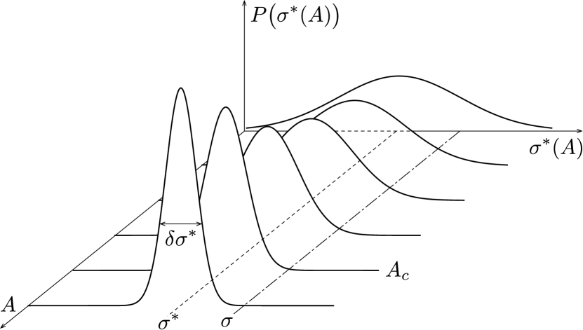
Figure 2: (Sketch) A patch of size $A$ has a strength $\sigma^{*}(A)$, which, due to disorder, is distributed around its thermodynamic value $\sigma^{*}$. Denoting $\delta\sigma^{*}(A)$ the width of this distribution for a given size $A$, $\delta\sigma^{*}$ will decrease as $A$ increases – a large patch has a better estimate of the true, thermodynamic, $\sigma^{*}$. Consequently, if an event is nucleated at $\sigma>\sigma^{*}$, disorder can still stop the event if its width $A$ is sufficiently small ($\delta\sigma^{*}$ is large for small $A$, so there is a finite probability that for that region in space $\sigma^{*}(A)>\sigma$). However, an event of size $A>A_{c}$ cannot be stopped by disorder, as the probability that that region in space has a strength $\sigma^{*}(A)>\sigma$ vanishes.

Geometry of avalanches

When slip occurs on a length scale $A$, the disorder characterising this region evolves. Locally, the interface strength can decrease by some increment $\delta\sigma^{*}(A)\sim A^{-\chi}$. Slip will stop when the local stress, proportional to $u/A$, decreases by a similar magnitude. It corresponds to a slip of order $u$ satisfying $u/A\sim A^{-\chi}$. Using that by definition $S\sim A^{d}u$ then leads to $S\sim A^{d_{f}}$ (Eq. 2) with:

$$d_{f}=d+1-\chi=d+\zeta.$$ (10)

Note that Eqs. 7, 9 and 10 are well known to hold in the absence of inertia and velocity weakening Fisher (1998). The proposition that they describe the pinning of velocity-weakening elastic materials, where avalanches co-exist with system-spanning events and where the flow curve has a minimum at finite slip rate, is to the best of our knowledge new. Indeed, most previous theoretical works argued that powerlaw avalanches would be absent in that case Fisher et al. (1997); Dahmen et al. (1998). Yet, the values of the exponents will differ in the absence or presence of large inertia, as we document below. We now turn to a scaling relation that is specific to the presence of velocity weakening.

Duration of avalanches

For stresses in the vicinity of $\sigma^{*}$, according to the flow curve sketched in Fig. 1B, slip is possible only if the slip rate lies in the vicinity of $\dot{u}_{\min}$. We make the hypothesis that within an avalanche, a sizeable fraction of the interface is slipping at any given point in time. The characteristic slip rate of an avalanche, $\dot{u}$, thus satisfies $\dot{u}\equiv S/(A^{d}T)\sim\dot{u}_{\min}$ that behaves as a constant as $\sigma\rightarrow\sigma^{*}$, which implies $T\sim A^{z}$ (Eq. 3) with:

$$z=d_{f}-d=\zeta$$ (11)

3 Testing the theory

3.1 A Rosetta Stone Model for frictional interfaces

We consider the minimal model of frictional interface containing disorder, long-range elasticity and inertia introduced in de Geus et al. (2019). Its details, as well as the dimensionless units we choose, are reviewed in the appendix. As illustrated in Fig. 3A, the frictional interface is discretised in $L$ (orange) “blocks” of unit size. Such a mesoscopic description is standard in Burridge-Knopoff type models Burridge and Knopoff (1967) or in the depinning literature Fisher et al. (1997). In the absence of inertia, it can successfully describe interfaces beyond the so-called “Larkin length” Cao et al. (2018), below which asperities always collectively rearrange and the details of the disorder matters. In the presence of velocity weakening, such a description can describe the interface beyond another length scale $L_{c}$, below which elastic forces dominate those stemming from velocity weakening Lebihain et al. (2021); Perfettini et al. (2003); Ray and Viesca (2017); Dublanchet (2018); Albertini et al. (2021); Schär et al. (2021); Uenishi and Rice (2003). Below, we estimate $L_{c}$ to be about 20 blocks in our model.

The interface is embedded within two homogeneous linear elastic bodies, of total height $\approx L$, modelled by finite elements (blue) . The system is driven at the top and fixed at the bottom, and presents periodic boundaries on the horizontal axis. Each block responds linear elastically up to a randomly chosen yield stress, whereupon it slips. This corresponds to a potential energy that, as a function of local slip, comprises a sequence of parabolic wells of random width, as illustrated in Fig. 3A. Disorder stems from randomly choosing the yield stresses, which are proportional to the width of the wells. In the absence of inertia, such models are used to study the depinning transition Jagla (2017), where they allow for fast simulations and a simple definition of avalanches, whose size $S$ is simply the number of times blocks rearranged within an event.

(A)

(B)

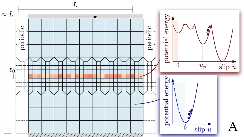
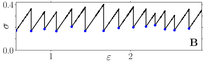
Figure 3: LABEL:sub@fig:model. The frictional interface is modelled using $L$ ‘blocks’ (finite elements in orange). The interface is embedded between two elastic bodies (also discretised using finite elements in blue) such that the entire system is approximately square. The potential energy of blocks along the interface and in the bulk are sketched as indicated. LABEL:sub@fig:typical. Macroscopic stress $\sigma$ vs strain $\varepsilon$ response to a quasistatic drive in which the top boundary is displaced ‘infinitely’ slowly. After each vanishingly small step, energy is minimised by following the inertial dynamics. The position of the top boundary and the reaction force yield $\varepsilon$ and $\sigma$ (see details about units in the appendix). ‘Events’, during which at least on block yields, are indicated with a marker, in blue when they are system spanning.

We consider standard inertial dynamics, with a small damping term chosen to ensure that elastic waves become damped after propagating on a length scale of order $\sim L$, modelling the leakage of heat at the system boundary. As we show below, the presence of (weakly damped) inertia leads to a velocity weakening, well fitted by rate-and-state description. Thus, this model is ideally suited to build a dictionary between the rate-and-state description (that focuses on velocity-weakening) and the depinning viewpoint (that focuses on disorder).

(A)

(B)

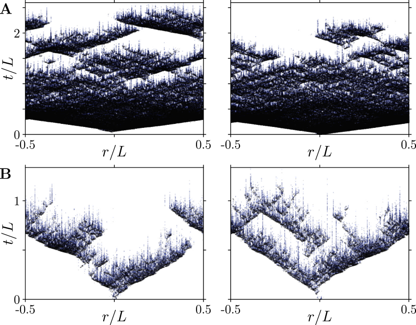
Figure 4: Event maps for two representative system-spanning events (LABEL:sub@fig:eventmap:a) and two large avalanches nucleated at $\sigma_{c}$ (LABEL:sub@fig:eventmap:b). A point is placed in time $t$ and space $r$ for each yield event (black if the block yields in the positive direction and blue if it yields in the negative direction).

3.2 Calibrating and testing rate-and-state

Stationary velocity weakening

Velocity-weakening is already apparent under a quasistatically imposed shear, where it leads to stick slip. As illustrated in Fig. 3B, system-spanning events drop the stress to some value indicated in blue, are punctuated by ‘avalanches’ in which a fraction of the blocks yield (small markers). Fig. 4A shows a spatiotemporal map of two system-spanning events spontaneously occurring upon loading (i.e. at large stress), whereas Fig. 4B illustrates two large avalanches (that we triggered directly after system spanning events, i.e. at low stress). For events nucleated at high stress, we show the average stress along the interface as a function of time in Fig. 5 . We use a blue contour to delimit the (average) event, using which we see that the stress drops significantly inside the event. Note that, in this work, we do not focus on the properties of the front (that travels at a velocity higher than the shear wave speed).

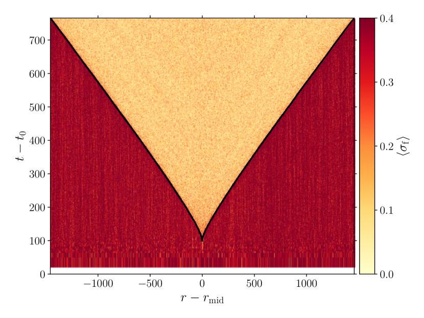
Figure 5: Ensemble average stress $\sigma_{\mathrm{f}}(r,t)$ (colour) along the weak layer $r$ (horizontal axis) as a function of time since the beginning of the event (vertical axis). The average is taken with respect to the (in general time-dependent) center of the event (details in appendix). Identically, the average number of times a block yielded, $s(r,t)$, is recorded, whose $s(r,t)=1$ contour is shown to delimit the front of the event.

To describe the observed velocity-weakening, we consider the rate-and-state description relating the interfacial stress $\sigma_{\mathrm{f}}$ as a function of slip rate $\dot{u}$ and time $t$ as: ${\sigma_{\mathrm{f}}=\sigma_{s}+a\ln(\dot{u})+b\ln(\theta(\dot{u},t))}$. Here, the time dependence enters implicitly through a ‘state’ parameter $\theta$. Furthermore, $\sigma_{s}$ is some offset and $a$ and $b$ are parameters. Usually, the state parameter is assumed to follow a simple linear ageing law $\dot{\theta}=1-\theta\dot{u}/D_{c}$. This equation captures that memory is lost once slip becomes larger than a distance $D_{c}$, beyond which the steady state ($\dot{\theta}=0$) is reached, which implies the stationary behaviour:

$$\sigma_{\mathrm{f}}=\sigma_{s}+(a-b)\ln(\dot{u}).$$ (12)

Note that in frictional experiments, the “state” parameter is often associated to the real contact area. This is not the case in our model, where the contact area is fixed. Instead, we think of the state parameter as characterising the mechanical noise stemming from inertia, that must take a finite time to reach a stationary equilibrium.

To calibrate Eq. 12, we measure the steady state interfacial stress $\sigma_{\mathrm{f}}$ for different imposed slip rates $\dot{u}$, averaged in both space and time. Measurements corresponds to the solid blue markers in Fig. 6. The solid blue line fits them according to Eq. 12, and leads to $a-b\simeq-0.03$ (and $\sigma_{s}\simeq 0.041$).

The dynamics are intermittent at imposed $\dot{u}<\dot{u}_{\min}$ (defined in Fig. 1B) , and stick slip occurs. The response $\sigma_{\mathrm{f}}(\dot{u})$ at small strain rate can be estimated by measuring evolution of the spatial average stress $\sigma_{\mathrm{f}}$ and the slip rate $\dot{u}$ along the weak layer in system-spanning events. After these events span the system, the average slip rate $\dot{u}$ slowly relaxes toward zero. These measurements corresponds to the light-blue points in Fig. 6 that also are well fitted by Eq. 12 with the same parameters.

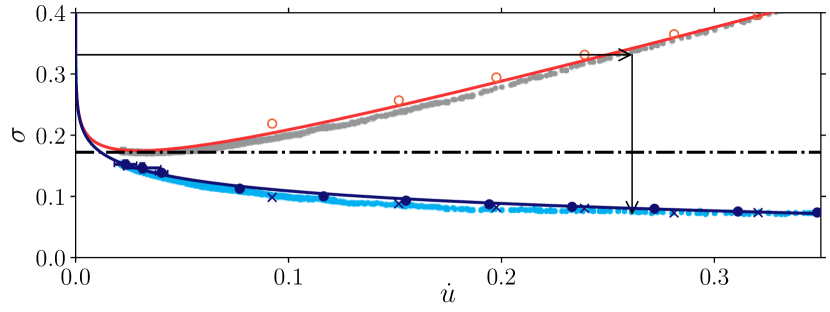
Figure 6: In blue (solid markers): Constitutive behaviour of the interfacial stress $\sigma_{\mathrm{f}}$ vs slip rate $\dot{u}$. The “rate-and-state” law, Eq. 12, is fitted on the solid blue markers that are measured in the steady state of a “flow experiment” in which the system is subjected to a constant shear rate. The fit is confirmed through a measurement of $(\sigma_{\mathrm{f}},\dot{u})$ during system-spanning events, as they stop ($\dot{u}$ decreases toward zero), as shown using light-blue points, truncated at low $\dot{u}$ when there are no more plastic events. In red (open markers): effective flow curve relating the far-field stress $\sigma$ to the local slip rate $\sigma=\sigma_{\mathrm{f}}(\dot{u})+\dot{u}$. The solid red curve corresponds to the fit obtained from the solid blue curve, while grey points are obtained from light-blue points. The cross-markers and open markers indicate respectively the measurements of $(\sigma_{\mathrm{f}},\dot{u})$ and $(\sigma,\dot{u})$ obtained by measuring the slip rate $\dot{u}$ and interfacial stress $\sigma_{\mathrm{f}}$ within a rupture occurring at an imposed stress $\sigma$. The minimum of the effective flow curve $\sigma_{\min}$ is indicated using a dash-dot line.

As mentioned in the introduction, in rate-and-state descriptions there is a characteristic length scale $L_{c}$ beyond which velocity-weakening effects are important. As recalled in the appendix, we can now estimate $L_{c}$ using the value of $a-b$ and a natural estimate for the slip $D_{c}$ where stationarity is reached. We assume that $D_{c}$ corresponds to the characteristic slip length for which plasticity occurs in a given block, i.e. the typical slip for which one exits the parabolic potential in Fig. 3A. With this, we obtain $L_{c}\approx 20$ blocks. In what follows, we focus on the quantification of slip events that are larger than $L_{c}$.

Radiation damping leads to a non-monotonic effective flow curve

The blue curve in Fig. 6 describes a stationary situation. However, when a slip event occurs and has not yet spanned the entire system, it must accelerate the elastic material around it. This phenomenon must obviously occur here as well, since we realistically describe the elastic material around the interface. Zheng and Rice (1998) show that it is captured by a “radiation damping” term, describing the difference between the stress in the far field $\sigma$ and that of the interface $\sigma_{\mathrm{f}}$ during an event that is growing in space. In our dimensionless units (see appendix), it simply reads:

$$\sigma=\sigma_{\mathrm{f}}(\dot{u})+\dot{u}.$$ (13)

We show the far-field stress $\sigma$ in red in Fig. 6. A key observation is that this curve is non-monotonic, and presents a minimum $\sigma_{\min}\approx 0.17$. Following previous works Zheng and Rice (1998); Brener et al. (2018), nucleation of a system-spanning, crack-like, event in homogeneous systems is possible beyond some stress $\sigma^{*}\approx\sigma_{\min}$. Below, we will support empirically our prediction that $\sigma^{*}$ is also the stress $\sigma_{c}$ where avalanches display a diverging cut-off.

Another prediction of rate-and-state (less relevant to our present purpose, but useful to further support the predictive power of rate-and-state in our model) is that when a system-spanning event starts to invade the material, away from the rupture front the local stress and slip rate can be readily extracted from Eq. 13, see Barras et al. (2019). This result is illustrated using the arrows in Fig. 6, showing that for a given imposed stress $\sigma$ (horizontal arrow), $\dot{u}$ and $\sigma_{\mathrm{f}}$ within system-spanning events can be read from this curve (vertical arrow). We confirm this construction in Fig. 6: the open markers indicate the applied stress $\sigma$ and the observed slip rate $\dot{u}$. The cross-markers instead indicate the interfacial stress $\sigma_{\mathrm{f}}$ inside the event and $\dot{u}$. We indeed find that $(\sigma_{\mathrm{f}},\dot{u})$ away from the rupture front closely follow the identified steady-state flow curve.

3.3 Statistics of slip events

We now test the (i) scaling relations we derived earlier for slip events and (ii) the correspondence between the stress $\sigma_{c}$ where avalanches diverge and the rate-and-state characteristic stress $\sigma_{\min}$, in the neighbourhood of which nucleation of unstable rupture front is predicted in homogeneous systems, at $\sigma^{*}\gtrsim\sigma_{\min}$ Brener et al. (2018).

Interface roughness

As discussed in the theoretical section, the fluctuation of the strength of the interface $\delta\sigma^{*}$ must be reflected in the fluctuations $\delta\sigma_{\mathrm{f}}$ of the physical stress carried by the interface, since slip will tend to occur until the mean stress in a region of size $A$, $\sigma_{\mathrm{f}}(A)$, has relaxed toward $\sigma^{*}(A)$. We have no direct measurement of $\sigma^{*}(A)$. Instead, we study $\sigma_{\mathrm{f}}(A)$ and its fluctuation $\delta\sigma_{\mathrm{f}}(A)$. we consider the system directly after 4000 system-spanning events , indicated in blue in Fig. 3B. We randomly choose patches of linear length $A$ along the interface, and compute the average stress in each patch. We then measure the mean and the standard deviation $\delta\sigma_{\mathrm{f}}(A)$ for different length $A$. In Fig. 7A, we confirm the powerlaw behaviour $\delta\sigma_{\mathrm{f}}(A)\sim A^{-\chi}$, from which we gain an estimate of the exponent $\chi$ entering Eq. 6 (assuming $\delta\sigma_{\mathrm{f}}(A)\approx\delta\sigma^{*}(A)$).

Such stress fluctuations must affect the roughness of the interface, as argued above. We confirm this view in Fig. 7B, which displays the relationship between the slip fluctuations $||u(r)-u(r^{\prime})||$ and the distance $||r-r^{\prime}||$. This observation confirms a powerlaw postulated in Eq. 5 with an exponent $\zeta\simeq 0.60$, a measurement consistent with the scaling relation $\chi={1-\zeta}$ of Eq. 7.

(A)

(B)

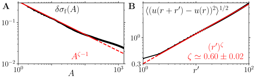
Figure 7: LABEL:sub@fig:zeta_stress. Standard deviation of the distribution of mean interfacial stress $\sigma_{\mathrm{f}}$ on a patch of blocks of size $A$ as a function of $A$. In particular, we measure $\text{std}(\{\sum_{i=j}^{j+A}\sigma_{i}/A\})$ (with $i$ the index of a block along the weak layer), with the set $\{\ldots\}$ coming from choosing $j$ at random locations in each realisation of the ensemble; see appendix for a precise statement. LABEL:sub@fig:zeta. Roughness exponent $\zeta$ measured from the mean square fluctuations of slip (note that a spatial average on $r$ is implied). The error bar on $\zeta$ includes both statistical errors (estimated from a least square regression) and systematic biases (estimated by reducing the fitting range), as detailed in the appendix.

Statistics of avalanches

To acquire a large statistics, we follow the strategy of de Geus et al. (2019) of manually triggering $9000$ events such as Fig. 4B, using a local perturbation at imposed strain, following a system spanning event. The post mortem effect of such an avalanche on the slip profile is shown in Fig. 8A, illustrating the definitions of the spatial extension $A$ and the total slip $S$. As shown in Figs. 8B, 8C and 8D, we confirm powerlaw behaviours for the distribution of avalanches $P(S)\sim S^{-\tau}$, the avalanche geometry $S\sim A^{d_{f}}$, and duration $T\sim A^{z}$; with $\tau\approx 1.77$, $z\approx 0.64$ and $d_{f}\approx 1.60$.

(A)

(B)

(C)

(D)

(E)

(F)

(G)

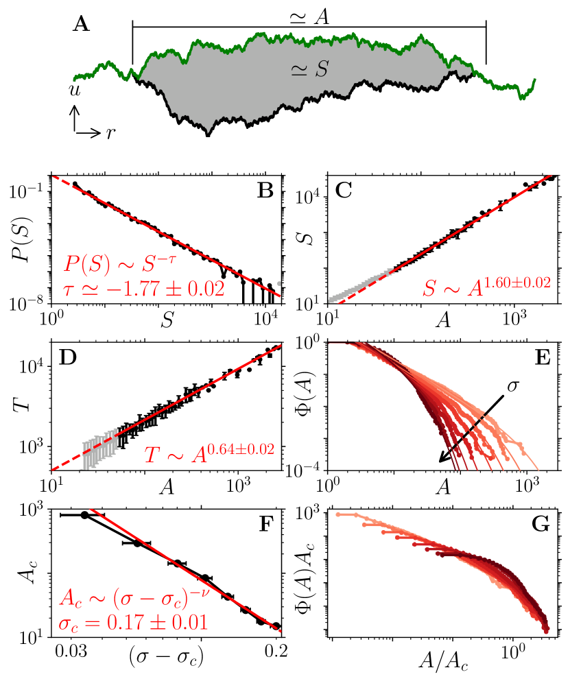
Figure 8: (LABEL:sub@fig:roughness-LABEL:sub@fig:TA) LABEL:sub@fig:roughness. Example of slip profile $u(r)$ before (bottom black curve) and after (top green curve) an avalanche. The linear extension $A$ and total slip $S$ are schematically indicated. Our results are consistent with $P(S)\sim S^{-\tau}$ (LABEL:sub@fig:PS), $S\sim A^{1+\zeta}$ (LABEL:sub@fig:SA), and avalanche duration $T\sim A^{\zeta}$ (LABEL:sub@fig:TA). LABEL:sub@fig:PhiA. Cumulative probability $\Phi(A)$ of avalanches (whose $A<L$) triggered at different stresses $\sigma$. The thin line indicates a fit $\Phi(A)\sim A^{1-\tau_{A}}\exp(-A/A_{c})$. Indeed, the obtained $A_{c}(\sigma)$ collapses our data (LABEL:sub@fig:nu). LABEL:sub@fig:PhiA_collapse. Fit of the offset $\sigma_{c}$ such that $A_{c}\sim(\sigma-\sigma_{c})^{-\nu}$, while imposing our prediction for $\nu$ in Eq. 9.

Nucleation size

To estimate the nucleation size $A_{c}$ beyond which an avalanche becomes a rupture front spanning the system, we measure the cumulative distribution of avalanche elongation $\Phi(A)$ at various stress levels, as shown in Fig. 8E. Next, we fit $\Phi(A)\sim A^{1-\tau_{A}}\exp(-A/A_{c})$ so as to extract $A_{c}$. In Fig. 8F, we confirm that rescaling $\Phi(A)$ by such an obtained $A_{c}$ indeed collapses the different curves. There is a considerable empirical indeterminacy on the exponent $\nu$ entering $A_{c}\sim(\sigma-\sigma_{c})^{-\nu}$, because the value of $\sigma_{c}$ is not known a priori. To proceed, we impose the predicted value $\nu=1/(1-\zeta)$ with $\zeta=0.60$ and choose $\sigma_{c}$ such as to obtain the best powerlaw behaviour, as displayed in Fig. 8F. We obtain a good fit, showing that $\nu$ is consistent with our prediction. Most importantly, we get $\sigma_{c}\approx 0.17\pm 0.01$ which is consistent with the value $\sigma_{\min}\approx 0.17$ extracted from the effective flow curve. Since rate-and-state predicts a threshold for unstable slip events at $\sigma^{*}\approx\sigma_{\min}$, our observations support that $\sigma^{*}$ indeed controls avalanches in disordered frictional interfaces.

Summary of Results

Table 1: Overview of results: scaling predictions and measured exponents in our $d=1$ system. We report the fitted exponents in Figs. 7 and 8. The uncertainty sums the statistical error plus an estimate of the systematic error stemming from the finite system size (which is estimated by considering the change in exponent in a twice smaller system).

Scaling	Prediction	Measurement
$P(S)\sim S^{-\tau}$	-	$1.77\pm 0.25$
$\delta u(r)\sim r^{\zeta}$	-	$0.60\pm 0.08$
$S\sim A^{d_{f}}$	$1+\zeta\simeq 1.60$	$1.60\pm 0.09$
$T\sim A^{z}$	$\zeta\simeq 0.60$	$0.64\pm 0.06$
$A_{c}\sim(\delta\sigma)^{-\nu}$	$1/(1-\zeta)\simeq 2.5$	$2.25\pm 0.77$

The set of exponents measured are reported in Table 1. $d_{f}$ and $z$ are in excellent agreement with our predictions ($\nu$ is nicely consistent with those, but cannot be extracted precisely).

These exponents differ markedly from those obtained in the absence of inertia with the same dimension $d=1$ and long-range interactions, for which it is found numerically that $\zeta\in[0.34,0.39]$ Ramanathan and Fisher (1998); Rosso and Krauth (2002); Middleton (1992); Narayan and Fisher (1993); Tanguy et al. (1998); Duemmer and Krauth (2007). These values are in reasonable agreement with renormalization group (RG) predictions Ertaş and Kardar (1994); Narayan and Fisher (1993); Chauve et al. (2001). However, RG has not been successfully developed when velocity weakening is important. In that case, our results indicate the existence of a new universality class.

At the experimental level, crack propagation Schmittbuhl and Måløy (1997); Tallakstad et al. (2011); Vincent-Dospital et al. (2021) and contact line experiments Prevost et al. (2002); Rubio et al. (1989) often report $\zeta\in[0.5,0.7]$. These exponents are closer to our predictions, yet it is unclear if inertia is responsible for this discrepancy with over-damped numerical observations Ramanathan and Fisher (1998); Rosso and Krauth (2002); Middleton (1992); Narayan and Fisher (1993); Tanguy et al. (1998); Duemmer and Krauth (2007), or if other effects are at play Vincent-Dospital et al. (2021).

4 Conclusion & perspective

Summary

We have introduced a theoretical framework for the nucleation and statistics of slip at a disordered frictional interface. It builds on rate-and-state results Zheng and Rice (1998); Brener et al. (2018) showing that in the presence of strong velocity-weakening effects, a homogeneous system presents a threshold stress $\sigma^{*}$ beyond which a rupture can invade the system. We have argued that in the presence of disorder, such a threshold must lead to powerlaw avalanches. Rupture occurs when one avalanche becomes larger than some size $A_{c}$ beyond which the disorder becomes negligible and cannot stop a rupture. $A_{c}$ diverges as $\sigma\rightarrow\sigma^{*}_{+}$ with some new exponent. This framework leads to quantitative predictions, partly based on extending arguments from the depinning literature Fisher (1998), where the threshold stress can be defined statically, to situations where the threshold is dynamically defined. Most importantly, our theoretical approach should stand as long as the frictional interface is well described by rate-and-state, irrespectively of the underlying mechanism causing velocity-weakening. Note that we have numerically checked this prediction only in a specific model, leaving a check to broader classes of models for future work.

Next, we used a minimal model of frictional interface as a Rosetta Stone, in which (i) rate-and-state equations can be calibrated and their predictions tested and (ii) disorder is easily controllable and slip statistics readily measurable. It allowed for a stringent test of our scaling predictions, and put forwards numerical values for exponents that future theories should seek to explain.

Geophysical data

We have argued that for a disordered but overall flat velocity-weakening frictional interface, the distribution of slip events should be bimodal. Powerlaw distributed avalanches are present, which display scaling properties. We find for example a scaling relationship between the avalanche size or “seismic moment” $S$ and its associated stress drop $\delta\sigma_{\mathrm{f}}\sim S^{-1/(d_{f}\nu)}\sim S^{-0.25}$. In the geophysics literature, these empirical facts are debated. Some studies report that the stress drop mildly decreases Shearer et al. (2006) or increases Trugman and Shearer (2017) with the earthquake size. Furthermore, as noted in the introduction, for a single fault bimodal Wesnousky (1994) or mono-modal Page et al. (2011) slip distributions have been argued for. In our opinion, the interpretation of these results is complicated by the geometry of faults, which display broadly distributed segments where slip can occur Manighetti et al. (2009). We view our theoretical results as a first step focusing on a simple interface geometry. Arguably, more complex geometrical factor must be included to rationalise geophysical observations. In this respect, it would be very interesting to consider a frictional interface made of powerlaw distributed segments. It can be readily implemented in our model, where the geometry of plastic regions where slip occurs can be chosen at will.

Future works

More generally, our methodology corresponds to a minimal model with a desired rate-and-state behaviour. In the future, controlled disorder can be used to incorporate other phenomena of interest, and study how they shape slip statistics. A particularly relevant case is thermal creep, which is expected to lead to an $N$-shaped effective flow curve, which can be readily obtained by simulating the dynamics in our model at finite temperature. Likewise, the materials surrounding the interface can be viscoelastic instead of elastic, which is a sufficient condition (but not always necessary Houdoux et al. (2021)) to obtain aftershocks Jagla et al. (2014).

Appendix A Details of the model

Equation of motion

We consider standard continuum elasto-dynamics, so that the equation of motion reads

$$\tilde{\rho}\partial_{\tilde{t}}^{2}\tilde{w}_{i}(r)=\mathrm{div}\big{(}\tilde{\sigma}_{ij}(r)\big{)}-\tilde{\alpha}\partial_{\tilde{t}}\tilde{w}_{i}(r)$$ (14)

where $\tilde{w}_{i}(r)$ is the displacement field (a function of position $r$, whose vectorial nature is omitted for notational simplicity), and $\partial_{\tilde{t}}\tilde{w}_{i}$ and $\partial_{\tilde{t}}^{2}\tilde{w}_{i}$ its first and second time derivative. $\tilde{\rho}$ is the mass density and $\tilde{\alpha}$ is the (small) damping coefficient, both are taken homogeneous. $\mathrm{div}\big{(}\tilde{\sigma}_{ij}(r)\big{)}$ is the divergence of the stress tensor $\tilde{\sigma}_{ij}$. The latter follows from linear elasticity, that we model

$$\tilde{\sigma}_{ij}(r) =(\tilde{\kappa}/(d+1))\mathrm{tr}\big{(}\tilde{\varepsilon}_{ij}(r)\big{)}\delta_{ij}$$ (15)

$$+2\tilde{\mu}(\tilde{u}(r)-\tilde{u}_{\text{min}}(r))N_{ij}(r).$$

Here, $\tilde{\varepsilon}_{ij}(r)=(\partial_{i}\tilde{w}_{j}(r)+\partial_{j}\tilde{w}_{i}(r))/2$ is the strain tensor. $d+1$ is the dimension of the bodies (here $d+1=2$), $\tilde{\kappa}$ is the bulk modulus, $\tilde{\mu}$ is the shear modulus; $\delta_{ij}$ is the unit tensor and $\mathrm{tr}(a_{ij})=a_{ij}\delta_{ij}$ is the trace of $a_{ij}$. $N_{ij}(r)$ defines the direction of shear as

$$N_{ij}(r)=\mathrm{dev}(\tilde{\varepsilon}_{ij}(r))/\tilde{u}(r)$$ (16)

where $\mathrm{dev}(\tilde{\varepsilon}_{ij}(r))$ is the deviatoric (trace-free) part of the strain tensor and

$$\tilde{u}(r) \equiv||\tilde{\varepsilon}_{ij}(r)||_{d}$$ (17)

$$\equiv(\mathrm{dev}(\tilde{\varepsilon}_{ij}(r))\mathrm{dev}(\tilde{\varepsilon}_{ij}(r))/2)^{1/2}$$

corresponds to the magnitude of the shear strain, that we refer to as “slip”. Likewise, we define the magnitude of shear stress

$$||\tilde{\sigma}_{ij}(r)||_{d}\equiv(2\,\mathrm{dev}(\tilde{\sigma}_{ij}(r))\mathrm{dev}(\tilde{\sigma}_{ij}(r))^{1/2}.$$ (18)

The potential energy landscape in Fig. 3A is defined along $\tilde{u}(r)$, with $\tilde{u}_{\text{min}}(r)$ the currently closest local minimum along the coordinate $\tilde{u}(r)$. It is always equal to zero in the bulk (in blue in Fig. 3A), but typically finite along the ‘weak’ layer (in red in Fig. 3A). Along that layer, the cusps are separated by a distance chosen randomly from a Weibull distribution, that has a typical value $2\tilde{u}_{0}$.

Units

A typical magnitude of shear strain is the typical yield strain $\tilde{u}_{0}$ of a block, that we use to define units, such that $\varepsilon_{ij}(r)\equiv\tilde{\varepsilon}_{ij}(r)/\tilde{u}_{0}$ and $\sigma_{ij}(r)\equiv\tilde{\sigma}_{ij}(r)/\tilde{\sigma}_{0}$ with $\tilde{\sigma}_{0}\equiv 4\tilde{\mu}\tilde{u}_{0}$. Thereby, we denote dimensionless quantities $\bullet$ and their dimension-full equivalent $\tilde{\bullet}$.

We define the plastic slip $u_{p}(r)\equiv\tilde{u}_{\min}(r)/\tilde{u}_{0}$ as the location of the current local minimum in dimensionless slip space, see Fig. 3A. These definitions are such that, on average, the number of times a block yields $s(r)=\Delta u_{p}(r)/2\approx\Delta u(r)/2$. The slip rate $\dot{u}\equiv\Delta u/\Delta t$, with time $t\equiv\tilde{t}/\tilde{t}_{0}$, where $\tilde{t}_{0}\equiv\tilde{\ell}_{0}/\tilde{c}_{s}$ with $\tilde{c}_{s}$ the shear wave speed. We note that length is expressed in units of $\tilde{\ell}_{0}$ such that $L\equiv\tilde{L}/\tilde{\ell}_{0}$ and $\ell_{0}\equiv\tilde{\ell}_{0}/\tilde{\ell}_{0}=1$. In our dimensionless units, slip at the interface, that we define as the strain in the blocks, thus coincides with the displacement discontinuity across the interface. Furthermore, time $t$ indicates the number of blocks a shear wave traversed. A slip rate $\dot{u}(r)=0.5$ thus indicates that a typical block yields once during time it takes a shear wave to travel the distance of one block.

We extract the total slip $S\equiv\int_{L}s(r)dr$ ($\int_{L}\ldots dr$ denotes the integral along the weak layer) as the total number of times blocks yield, $A$ the number of blocks that yield at least once (thus $A\equiv\int_{L}(s(r)+|s(r)|)/(2|s(r)|)dr$), and $T$ the (dimensionless) duration between the first and the last time that a block yield during an event.

Numerical model

The numerical treatment of this equation of motion corresponds to a discretisation in space using finite elements (where at the weak layer the elements coincide with the blocks of linear size $\tilde{\ell}_{0}$, see Fig. 3A), and in time using the velocity Verlet algorithm. The numerical values of all parameters, and more details, can be found in de Geus et al. [2019], de Geus [2019]. Different from those references, here we consider a bigger system of $L=4\times 3^{6}$ blocks (except for the results in Fig. 4 which are made on the system of de Geus et al. [2019]), and a ten times smaller typical strain $\tilde{u}_{0}$ to acquire more events per realisation while respecting the small strain assumption. Note that this does not lead to any change in terms of the dimensionless quantities reported here and in de Geus et al. [2019]. In addition, we perform flow experiments by imposing a fixed shear rate to the top boundary. In practice, the shear is supplied to the system in a distributed manner, such that in each time step all nodal displacements are updated according to an affine simple shear, though only the top boundary is fixed. We measure both $\sigma_{\mathrm{f}}$ and $\dot{u}$ as averaged in space along the interface and on a finite window of time deep in the steady state, as well as on different realisations.

Quantities

The remote stress is the volume averaged shear stress

$$\sigma\equiv\left|\left|\iint_{L}\bm{\sigma}(\vec{r})\,d\vec{r}\,\right|\right|_{d}=\sum_{\beta=1}^{n}(\tilde{f}_{x})_{\beta}/(n\tilde{\ell}_{0}\tilde{\sigma}_{0})$$ (19)

with $\bm{\sigma}(\vec{r})$ the adimensional stress tensor at a position $\vec{r}$ in $(d+1)$-dimensional space, and $\iint_{L}\ldots dr$ the integral over the entire domain in $(d+1)$-dimensional space. $(\tilde{f}_{x})_{\beta}$ are the reaction forces in horizontal direction of the $n+1$ nodes along the top boundary (one node is ‘virtual’ because of the periodic boundary conditions in horizontal direction) whose position is prescribed. The remote strain is the volume averaged strain

$$\varepsilon\equiv\left|\left|\iint_{L}\bm{\varepsilon}(\vec{r})\,d\vec{r}\,\right|\right|_{d}=(\tilde{w}_{x})_{\beta}/(\tilde{H}\tilde{u}_{0})$$ (20)

with $(\tilde{w}_{x})_{\beta}$ the displacement in horizontal direction of one of the nodes along the top boundary (the displacement of all of these nodes is definition equal), and $\tilde{H}\approx L\tilde{\ell}_{0}$ the actual height of the sample.

The stress along the interface

$$\sigma_{\mathrm{f}}\equiv\left|\left|\int_{L}\bm{\sigma}(r)\,dr\,\right|\right|_{d}=\left|\left|\sum_{i=1}^{L}\bm{\sigma}_{i}\,\right|\right|_{d}$$ (21)

with $i$ referring the block index along the weak layer (numbered from left to right). We note that

$$\sigma_{\mathrm{f}}(A)=\left|\left|\sum_{i=j}^{i+A}\bm{\sigma}_{i}\,\right|\right|_{d}.$$ (22)

(where periodicity implies $\bm{\sigma}_{i}=\bm{\sigma}_{i+L}$).

The slip along the interface

$$u\equiv\left|\left|\int_{L}\bm{\varepsilon}(r)\,dr\,\right|\right|_{d}=\left|\left|\sum_{i=1}^{L}\bm{\varepsilon}_{i}\,\right|\right|_{d}.$$ (23)

Finally, the slip rate

$$\dot{u}\equiv\left|\left|\int_{L}\,\partial_{t}\bm{\varepsilon}(r)\,dr\,\right|\right|_{d}=\left|\left|\sum_{i=1}^{L}\partial_{t}\bm{\varepsilon}_{i}\,\right|\right|_{d}.$$ (24)

Radiation damping

A nucleating event, whereby part of the interface and bulk are still static as the rupture invades the interface, is stabilised by the bulk surrounding it: to increase the slip rate $\dot{u}$ the bulk around the rupture has to be accelerated. Due to the cost of accelerating an expanding volume, the interfacial stress $\sigma_{\mathrm{f}}$ inside the event differs from the remote stress $\sigma$. Because the bulk is accelerated by elastic waves that radiate away from the interface this effect is commonly referred to as “radiation damping”. We emphasise that this is an effect of standard elasto-dynamics: it is not added by hand to our model.

The effect of radiation damping corresponds to a ‘cost’ of stress Zheng and Rice [1998] $\Delta\tilde{\sigma}_{xy}=\tilde{v}\tilde{\mu}/(2\tilde{c}_{s})$, with $\tilde{v}\equiv 2\Delta(\delta\tilde{r}_{x})/\Delta\tilde{t}$ Barras et al. [2020] the rate of change of the displacement discontinuity $\delta\tilde{r}_{x}\equiv 2\tilde{\varepsilon}_{xy}\tilde{\ell}_{0}=2\tilde{u}\tilde{\ell}_{0}$ such that $\Delta\tilde{\sigma}=(4\Delta\tilde{u}\tilde{\ell}_{0}/\Delta\tilde{t})(\tilde{\mu}/\tilde{c}_{s})=4\tilde{\mu}\Delta\tilde{u}/(\Delta\tilde{t}/\tilde{t}_{0})$ or $\Delta\tilde{\sigma}/(4\tilde{\mu}\tilde{u}_{0})=(\Delta\tilde{u}/\tilde{u}_{0})/(\Delta\tilde{t}/\tilde{t}_{0})$ and thus $\Delta\sigma=\dot{u}$.

Computation of $L_{c}$

For the rate-and-state law $\tilde{L}_{c}=-\pi\tilde{\mu}\tilde{D}_{c}/(\dot{\tilde{u}}\partial\tilde{\sigma}/\partial\dot{\tilde{u}})$ Brener et al. [2018] with $\partial\tilde{\sigma}/\partial\dot{\tilde{u}}=(\tilde{a}-\tilde{b})/\dot{\tilde{u}}$ the derivative of the steady state in Eq. 12, such that $\tilde{L}_{c}=-\pi\tilde{\mu}\tilde{D}_{c}/(\tilde{a}-\tilde{b})$. In our model, a block, on average, loses memory over a sliding distance $\tilde{D}_{c}=\tilde{u}_{0}\tilde{\ell}_{0}$. Using, furthermore, our units of stress such that $a=\tilde{a}/\tilde{\sigma}_{0}$ and $b=\tilde{b}/\tilde{\sigma}_{0}$, we find $\tilde{L}_{c}=-\pi\tilde{\mu}\tilde{u}_{0}\tilde{\ell}_{0}/(\tilde{\sigma}_{0}(a-b))=-\pi\tilde{\ell}_{0}/(4(a-b))$, and thus $L_{c}=-\pi/(4(a-b))\approx 26$.

Powerlaw fits

The powerlaw fit of $y=cx^{b}$ is performed using a least square fit of the linear relation $z\equiv\ln y=\ln c+b\ln x$. In the case of an uncertainty $\delta y$ (typically a standard deviation) we assume that $\delta y\ll y$ such that we use $\delta z=\delta y/y$. The error of the fitted exponent, $\delta b_{f}$, is then the square root of the relevant component at the diagonal of the 2x2 covariance matrix. Where possible, we also compute the fluctuations of the exponent, $\delta b_{\ell}$, by reducing the fitting range by a factor of two and four. We report $\delta b_{\ell}$ in Fig. 7B, and $\delta b_{f}$ in Figs. 8B, 8C and 8D (in Figs. 8B and 8C the $\delta b_{\ell}$ was simply found lower or equal to $\delta b_{\ell}$; in Fig. 8D the range is not sufficient to be reduced).

In Fig. 8F we account for the error in $\sigma$ by taking the error as dimensionless, allowing us to compose it in equal amounts of the errors in $\sigma$ (the standard deviation of $\sigma$ in each bin) and in $A_{c}$ (the fitting error from Fig. 8E). We use this protocol also to fit $\nu$ given $\sigma_{\min}\approx 0.17$ as reported in Table 1.

In Table 1 we estimate the error on $\nu$ as the difference between our prediction and a fit of the exponent of the data in Fig. 8F using $\sigma_{c}$ defined as the bottom of the effective flow curve in Fig. 6.

References

- Rice [1993] J.R. Rice. Spatio-temporal complexity of slip on a fault. J. Geophys. Res., 98(B6):9885, 1993. 10.1029/93JB00191.
- Scholz [1998] C.H. Scholz. Earthquakes and friction laws. Nature, 391(6662):37–42, 1998. 10.1038/34097.
- Xia et al. [2004] K. Xia, A.J. Rosakis, and H. Kanamori. Laboratory Earthquakes: The Sub-Rayleigh-to-Supershear Rupture Transition. Science, 303(5665):1859–1861, 2004. 10.1126/science.1094022.
- Rubinstein et al. [2004] S.M. Rubinstein, G. Cohen, and J. Fineberg. Detachment fronts and the onset of dynamic friction. Nature, 430(7003):1005–1009, 2004. 10.1038/nature02830.
- Ben-David et al. [2010] O. Ben-David, S.M. Rubinstein, and J. Fineberg. Slip-stick and the evolution of frictional strength. Nature, 463(7277):76–79, 2010. 10.1038/nature08676.
- Passelègue et al. [2013] F.X. Passelègue, A. Schubnel, S.B. Nielsen, H.S. Bhat, and R. Madariaga. From Sub-Rayleigh to Supershear Ruptures During Stick-Slip Experiments on Crustal Rocks. Science, 340(6137):1208–1211, 2013. 10.1126/science.1235637.
- Heaton [1990] T.H. Heaton. Evidence for and implications of self-healing pulses of slip in earthquake rupture. Phys. Earth Planet. In., 64(1):1–20, 1990. 10.1016/0031-9201(90)90002-F.
- Zheng and Rice [1998] G. Zheng and J.R. Rice. Conditions under which velocity-weakening friction allows a self-healing versus a cracklike mode of rupture. Bull. Seismol. Soc. Am., 88(6):1466–1483, 1998.
- Roch et al. [2022] T. Roch, E.A. Brener, J.-F. Molinari, and E. Bouchbinder. Velocity-driven frictional sliding: Coarsening and steady-state pulses. J. Mech. Phys. Solids, 158:104607, 2022. 10.1016/j.jmps.2021.104607. arxivid: 2104.13110.
- Svetlizky and Fineberg [2014] I. Svetlizky and J. Fineberg. Classical shear cracks drive the onset of dry frictional motion. Nature, 509(7499):205–208, 2014. 10.1038/nature13202.
- Svetlizky et al. [2016] I. Svetlizky, D. Pino Muñoz, M. Radiguet, D.S. Kammer, J.-F. Molinari, and J. Fineberg. Properties of the shear stress peak radiated ahead of rapidly accelerating rupture fronts that mediate frictional slip. Proc. Natl. Acad. Sci., 113(3):542–547, 2016. 10.1073/pnas.1517545113.
- Ben-David and Fineberg [2011] O. Ben-David and J. Fineberg. Static Friction Coefficient Is Not a Material Constant. Phys. Rev. Lett., 106(25):254301, 2011. 10.1103/PhysRevLett.106.254301. arxivid: 1104.5479.
- Popov [2010] V.L. Popov. Contact Mechanics and Friction. Springer Berlin Heidelberg, 2010. ISBN 978-3-642-10802-0. 10.1007/978-3-642-10803-7.
- Rabinowicz [1992] E. Rabinowicz. Friction coefficients of noble metals over a range of loads. Wear, 159(1):89–94, 1992. 10.1016/0043-1648(92)90289-K.
- Brace and Byerlee [1966] W.F. Brace and J.D. Byerlee. Stick-Slip as a Mechanism for Earthquakes. Science, 153(3739):990–992, 1966. 10.1126/science.153.3739.990.
- Gutenberg and Richter [1954] B.U. Gutenberg and C.F. Richter. Seismicity of the Earth and Related Phenomena. Princeton (NJ), 1954.
- Wesnousky [1994] S.G. Wesnousky. The Gutenberg-Richter or characteristic earthquake distribution, which is it? Bull. Seismol. Soc. Am., 84(6):1940–1959, 1994. 10.1785/BSSA0840061940.
- Page et al. [2011] M.T. Page, D. Alderson, and J. Doyle. The magnitude distribution of earthquakes near Southern California faults. J. Geophys. Res., 116(B12):B12309, 2011. 10.1029/2010JB007933.
- Manighetti et al. [2009] I. Manighetti, D. Zigone, M. Campillo, and F. Cotton. Self-similarity of the largest-scale segmentation of the faults: Implications for earthquake behavior. Earth Planet. Sci. Lett., 288(3-4):370–381, 2009. 10.1016/j.epsl.2009.09.040.
- Scholz and Engelder [1976] C.H. Scholz and J.T. Engelder. The role of asperity indentation and ploughing in rock friction — I. Int. J. Rock Mech. Min. Sci. Geomech. Abstr., 13(5):149–154, 1976. 10.1016/0148-9062(76)90819-6.
- Baumberger and Caroli [2006] T. Baumberger and C. Caroli. Solid friction from stick–slip down to pinning and aging. Adv. Phys., 55(3-4):279–348, 2006. 10.1080/00018730600732186. arxivid: cond-mat/0506657.
- Rabinowicz [1956] E. Rabinowicz. Stick and Slip. Sci. Am., 194(5):109–118, 1956.
- Marone [1998] C. Marone. Laboratory-derived friction laws and their application to seismic faulting. Annu. Rev. Earth Planet. Sci., 26(1):643–696, 1998. 10.1146/annurev.earth.26.1.643.
- Heslot et al. [1994] F. Heslot, T. Baumberger, B. Perrin, B. Caroli, and C. Caroli. Creep, stick-slip, and dry-friction dynamics: Experiments and a heuristic model. Phys. Rev. E, 49(6):4973–4988, 1994. 10.1103/PhysRevE.49.4973.
- Vincent-Dospital et al. [2020] T. Vincent-Dospital, R. Toussaint, S. Santucci, L. Vanel, D. Bonamy, L. Hattali, A. Cochard, E.G. Flekkøy, and K.J. Måløy. How heat controls fracture: The thermodynamics of creeping and avalanching cracks. Soft Matter, 16(41):9590–9602, 2020. 10.1039/D0SM01062F. arxivid: 1905.07180.
- Fisher et al. [1997] D.S. Fisher, K.A. Dahmen, S. Ramanathan, and Y. Ben-Zion. Statistics of Earthquakes in Simple Models of Heterogeneous Faults. Phys. Rev. Lett., 78(25):4885–4888, 1997. 10.1103/PhysRevLett.78.4885. arxivid: cond-mat/9703029.
- Ramanathan et al. [1997] S. Ramanathan, D. Ertaş, and D.S. Fisher. Quasistatic Crack Propagation in Heterogeneous Media. Phys. Rev. Lett., 79(5):873–876, 1997. 10.1103/PhysRevLett.79.873. arxivid: cond-mat/9611196.
- Schwarz and Fisher [2001] J.M. Schwarz and D.S. Fisher. Depinning with Dynamic Stress Overshoots: Mean Field Theory. Phys. Rev. Lett., 87(9):096107, 2001. 10.1103/PhysRevLett.87.096107. arxivid: cond-mat/0012246.
- Salerno et al. [2012] K.M. Salerno, C.E. Maloney, and M.O. Robbins. Avalanches in Strained Amorphous Solids: Does Inertia Destroy Critical Behavior? Phys. Rev. Lett., 109(10):105703, 2012. 10.1103/PhysRevLett.109.105703. arxivid: 1204.5965v1.
- Dieterich [1979] J.H. Dieterich. Modeling of rock friction: 1. Experimental results and constitutive equations. J. Geophys. Res., 84(B5):2161, 1979. 10.1029/JB084iB05p02161.
- Rice and Ruina [1983] J.R. Rice and A.L. Ruina. Stability of Steady Frictional Slipping. J. Appl. Mech., 50(2):343–349, 1983. 10.1115/1.3167042.
- Ruina [1983] A.L. Ruina. Slip instability and state variable friction laws. J. Geophys. Res. Solid Earth, 88(B12):10359–10370, 1983. 10.1029/JB088iB12p10359.
- Lebihain et al. [2021] M. Lebihain, T. Roch, M. Violay, and J.-F. Molinari. Earthquake Nucleation Along Faults With Heterogeneous Weakening Rate. Geophys. Res. Lett., 48(21), 2021. 10.1029/2021GL094901. arxivid: 2102.10870.
- Perfettini et al. [2003] H. Perfettini, M. Campillo, and I. Ionescu. On the scaling of the slip weakening rate of heterogeneous faults. J. Geophys. Res., 108(B9), 2003. 10.1029/2002JB001969.
- Ray and Viesca [2017] S. Ray and R.C. Viesca. Earthquake Nucleation on Faults With Heterogeneous Frictional Properties, Normal Stress. J. Geophys. Res. Solid Earth, 122(10):8214–8240, 2017. 10.1002/2017JB014521.
- Dublanchet [2018] P. Dublanchet. The dynamics of earthquake precursors controlled by effective friction. Geophys. J. Int., 212(2):853–871, 2018. 10.1093/gji/ggx438.
- Albertini et al. [2021] G. Albertini, S. Karrer, M.D. Grigoriu, and D.S. Kammer. Stochastic properties of static friction. J. Mech. Phys. Solids, 147:104242, 2021. 10.1016/j.jmps.2020.104242. arxivid: 2005.06113.
- Schär et al. [2021] S. Schär, G. Albertini, and D.S. Kammer. Nucleation of frictional sliding by coalescence of microslip. Int. J. Solids Struct., 225:111059, 2021. 10.1016/j.ijsolstr.2021.111059. arxivid: 2010.04343.
- Ohnaka and Kuwahara [1990] M. Ohnaka and Y. Kuwahara. Characteristic features of local breakdown near a crack-tip in the transition zone from nucleation to unstable rupture during stick-slip shear failure. Tectonophysics, 175(1-3):197–220, 1990. 10.1016/0040-1951(90)90138-X.
- Brener et al. [2018] E.A. Brener, M. Aldam, F. Barras, J.F. Molinari, and E. Bouchbinder. Unstable Slip Pulses and Earthquake Nucleation as a Nonequilibrium First-Order Phase Transition. Phys. Rev. Lett., 121(23):234302, 2018. 10.1103/PhysRevLett.121.234302. arxivid: 1807.06890.
- Fisher [1983] D.S. Fisher. Threshold Behavior of Charge-Density Waves Pinned by Impurities. Phys. Rev. Lett., 50(19):1486–1489, 1983. 10.1103/PhysRevLett.50.1486.
- Fisher [1998] D.S. Fisher. Collective transport in random media: From superconductors to earthquakes. Phys. Rep., 301(1-3):113–150, 1998. 10.1016/S0370-1573(98)00008-8. arxivid: cond-mat/9711179.
- Dahmen et al. [1998] K.A. Dahmen, D. Ertaş, and Y. Ben-Zion. Gutenberg-Richter and characteristic earthquake behavior in simple mean-field models of heterogeneous faults. Phys. Rev. E, 58(2):1494–1501, 1998. 10.1103/PhysRevE.58.1494. arxivid: cond-mat/9803057.
- Schwarz and Fisher [2003] J.M. Schwarz and D.S. Fisher. Depinning with dynamic stress overshoots: A hybrid of critical and pseudohysteretic behavior. Phys. Rev. E, 67(2):021603, 2003. 10.1103/PhysRevE.67.021603. arxivid: cond-mat/0204623.
- Maimon and Schwarz [2004] R. Maimon and J.M. Schwarz. Continuous Depinning Transition with an Unusual Hysteresis Effect. Phys. Rev. Lett., 92(25):255502, 2004. 10.1103/PhysRevLett.92.255502.
- Baldassarri et al. [2006] A. Baldassarri, F. Dalton, A. Petri, S. Zapperi, G. Pontuale, and L. Pietronero. Brownian Forces in Sheared Granular Matter. Phys. Rev. Lett., 96(11):118002, 2006. 10.1103/PhysRevLett.96.118002. arxivid: cond-mat/0507533.
- de Geus et al. [2019] T.W.J. de Geus, M. Popović, W. Ji, A. Rosso, and M. Wyart. How collective asperity detachments nucleate slip at frictional interfaces. Proc. Natl. Acad. Sci., 116(48):23977–23983, 2019. 10.1073/pnas.1906551116. arxivid: 1904.07635.
- Gutenberg and Richter [1944] B. Gutenberg and C.F. Richter. Frequency of earthquakes in California. Bull. Seismol. Soc. Am., 34(4):185–188, 1944. 10.1785/BSSA0340040185.
- Kagan [2014] Y.Y. Kagan. Earthquakes: Models, Statistics, Testable Forecasts. John Wiley & Sons Inc, 2014. ISBN 978-1-118-63789-0 978-1-118-63788-3.
- Chayes et al. [1986] J.T. Chayes, L. Chayes, D.S. Fisher, and T. Spencer. Finite-Size Scaling and Correlation Lengths for Disordered Systems. Phys. Rev. Lett., 57(24):2999–3002, 1986. 10.1103/PhysRevLett.57.2999.
- Burridge and Knopoff [1967] R. Burridge and L. Knopoff. Model and theoretical seismicity. Bull. Seismol. Soc. Am., 57(3):341–371, 1967.
- Cao et al. [2018] X. Cao, S. Bouzat, A.B. Kolton, and A. Rosso. Localization of soft modes at the depinning transition. Phys. Rev. E, 97(2):022118, 2018. 10.1103/PhysRevE.97.022118. arxivid: 1705.10289.
- Uenishi and Rice [2003] K. Uenishi and J.R. Rice. Universal nucleation length for slip-weakening rupture instability under nonuniform fault loading. J. Geophys. Res. Solid Earth, 108(B1), 2003. 10.1029/2001JB001681.
- Langer et al. [1996] J.S. Langer, J.M. Carlson, C.R. Myers, and B.E. Shaw. Slip complexity in dynamic models of earthquake faults. Proc. Natl. Acad. Sci., 93(9):3825–3829, 1996. 10.1073/pnas.93.9.3825.
- Jagla [2017] E.A. Jagla. Different universality classes at the yielding transition of amorphous systems. Phys. Rev. E, 96(2):023006, 2017. 10.1103/PhysRevE.96.023006. arxivid: 1701.03324.
- Barras et al. [2019] F. Barras, M. Aldam, T. Roch, E.A. Brener, E. Bouchbinder, and J.-F. Molinari. Emergence of Cracklike Behavior of Frictional Rupture: The Origin of Stress Drops. Phys. Rev. X, 9(4):041043, 2019. 10.1103/PhysRevX.9.041043. arxivid: 1906.11533.
- Ramanathan and Fisher [1998] S. Ramanathan and D.S. Fisher. Onset of propagation of planar cracks in heterogeneous media. Phys. Rev. B, 58(10):6026–6046, 1998. 10.1103/PhysRevB.58.6026. arxivid: cond-mat/9712181.
- Rosso and Krauth [2002] A. Rosso and W. Krauth. Roughness at the depinning threshold for a long-range elastic string. Phys. Rev. E, 65(2):025101, 2002. 10.1103/PhysRevE.65.025101. arxivid: cond-mat/0107527.
- Middleton [1992] A.A. Middleton. Asymptotic uniqueness of the sliding state for charge-density waves. Phys. Rev. Lett., 68(5):670–673, 1992. 10.1103/PhysRevLett.68.670.
- Narayan and Fisher [1993] O. Narayan and D.S. Fisher. Threshold critical dynamics of driven interfaces in random media. Phys. Rev. B, 48(10):7030–7042, 1993. 10.1103/PhysRevB.48.7030.
- Tanguy et al. [1998] A. Tanguy, M. Gounelle, and S. Roux. From individual to collective pinning: Effect of long-range elastic interactions. Phys. Rev. E, 58(2):1577–1590, 1998. 10.1103/PhysRevE.58.1577. arxivid: cond-mat/9804105.
- Duemmer and Krauth [2007] O. Duemmer and W. Krauth. Depinning exponents of the driven long-range elastic string. J. Stat. Mech., 2007(01):P01019–P01019, 2007. 10.1088/1742-5468/2007/01/P01019.
- Ertaş and Kardar [1994] D. Ertaş and M. Kardar. Critical dynamics of contact line depinning. Phys. Rev. E, 49(4):R2532–R2535, 1994. 10.1103/PhysRevE.49.R2532. arxivid: cond-mat/9401027.
- Chauve et al. [2001] P. Chauve, P. Le Doussal, and K. Jörg Wiese. Renormalization of Pinned Elastic Systems: How Does It Work Beyond One Loop? Phys. Rev. Lett., 86(9):1785–1788, 2001. 10.1103/PhysRevLett.86.1785. arxivid: cond-mat/0006056.
- Schmittbuhl and Måløy [1997] J. Schmittbuhl and K.J. Måløy. Direct Observation of a Self-Affine Crack Propagation. Phys. Rev. Lett., 78(20):3888–3891, 1997. 10.1103/PhysRevLett.78.3888.
- Tallakstad et al. [2011] K.T. Tallakstad, R. Toussaint, S. Santucci, J. Schmittbuhl, and K.J. Måløy. Local dynamics of a randomly pinned crack front during creep and forced propagation: An experimental study. Phys. Rev. E, 83(4):046108, 2011. 10.1103/PhysRevE.83.046108. arxivid: 1205.6197.
- Vincent-Dospital et al. [2021] T. Vincent-Dospital, A. Cochard, S. Santucci, K.J. Måløy, and R. Toussaint. Thermally activated intermittent dynamics of creeping crack fronts along disordered interfaces. Sci Rep, 11(1):20418, 2021. 10.1038/s41598-021-98556-x.
- Prevost et al. [2002] A. Prevost, E. Rolley, and C. Guthmann. Dynamics of a helium-4 meniscus on a strongly disordered cesium substrate. Phys. Rev. B, 65(6):064517, 2002. 10.1103/PhysRevB.65.064517.
- Rubio et al. [1989] M.A. Rubio, C.A. Edwards, A. Dougherty, and J.P. Gollub. Self-affine fractal interfaces from immiscible displacement in porous media. Phys. Rev. Lett., 63(16):1685–1688, 1989. 10.1103/PhysRevLett.63.1685.
- Shearer et al. [2006] P.M. Shearer, G.A. Prieto, and E. Hauksson. Comprehensive analysis of earthquake source spectra in southern California. J. Geophys. Res., 111(B6), 2006. 10.1029/2005JB003979.
- Trugman and Shearer [2017] D.T. Trugman and P.M. Shearer. Application of an improved spectral decomposition method to examine earthquake source scaling in Southern California: EARTHQUAKE SOURCE SCALING IN SOUTHERN CALIFORNIA. J. Geophys. Res. Solid Earth, 122(4):2890–2910, 2017. 10.1002/2017JB013971.
- Houdoux et al. [2021] D. Houdoux, A. Amon, D. Marsan, J. Weiss, and J. Crassous. Micro-slips in an experimental granular shear band replicate the spatiotemporal characteristics of natural earthquakes. Commun Earth Environ, 2(1):90, 2021. 10.1038/s43247-021-00147-1.
- Jagla et al. [2014] E.A. Jagla, F.P. Landes, and A. Rosso. Viscoelastic Effects in Avalanche Dynamics: A Key to Earthquake Statistics. Phys. Rev. Lett., 112(17):174301, 2014. 10.1103/PhysRevLett.112.174301. arxivid: 1310.5051.
- de Geus [2019] T.W.J. de Geus. Supporting data: “How collective asperity detachments nucleate slip at frictional interfaces”. Zenodo, 2019. 10.5281/zenodo.3477938.
- Barras et al. [2020] F. Barras, M. Aldam, T. Roch, E.A. Brener, E. Bouchbinder, and J.-F. Molinari. The emergence of crack-like behavior of frictional rupture: Edge singularity and energy balance. Earth Planet. Sci. Lett., 531:115978, 2020. 10.1016/j.epsl.2019.115978. arxivid: 1907.04376.