A note on a modified fractional Maxwell model

Abstract.

In this paper we consider a modified fractional Maxwell model based on the application of Hadamard-type fractional derivatives. The model is physically motivated by the fact that we can take into account at the same time memory effects and the time-dependence of the viscosity coefficient. We obtain an ultra-slow relaxation response whose explicit analytic form is given by the Mittag-Leffler function with a logarithmic argument. We show graphically the main properties of this relaxation response, also with the asymptotic behaviour.

This paper has been published in Chaos, Solitons and Fractals, Vol 103 (2022) 112544/1-5. DOI: 10.1016/j.chaos.2022.112544

1. Introduction

Classical viscoelastic models are based on the combination of viscous dashpots and springs (in series or parallel), leading to different governing equations. The viscosity is considered as a constant in the classical models but in recent papers a time-varying viscosity $\eta(t)$ was introduced, we refer in particular to Pandey and Holm [20] and Yang et al.[25]. According to [25] a modified Maxwell model based on a time-varying viscosity can be formulated as

(1.1) $$\sigma+\frac{\eta(t)}{E}\frac{d\sigma}{dt}=\eta(t)\frac{d\epsilon}{dt},$$

where $\sigma$ and $\epsilon$ are the stress and the strain respectively, while $E$ is the elastic modulus of the spring.
The authors in [20], [25] have considered, in particular, a linearly time-varying viscosity

$$\eta(t)=\eta_{0}+\theta t,$$

where $\eta_{0}$ denotes the initial viscosity and $\theta$ the strain-hardening coefficient.
In this case the modified Maxwell model becomes

(1.2) $$\sigma+\frac{\eta_{0}+\theta t}{E}\frac{d\sigma}{dt}=\left(\eta_{0}+\theta t\right)\frac{d\epsilon}{dt}.$$

On the other hand, it is well-known that viscoelastic and mechanical models with memory based on the applications of fractional derivatives and integrals are widely used and also validated (we refer for example to [18], [22] and the references therein).
In the recent paper by Garra, Mainardi and Spada [7], the authors have considered a modified Lomnitz model based on the application of Hadamard-type integro-differential operators. Here we consider a little modification of the operator considered in [7] that is, for $\nu\in(0,1)$

(1.3) $$\begin{array}[]{ll}\widehat{O}^{t}_{\nu}f(t)&:={\displaystyle\frac{1}{\Gamma(1-\nu)}}\left(\frac{E}{\theta}\right)^{-\nu}\displaystyle\int_{\frac{1-\eta_{0}}{\theta}}^{t}\!\!\ln^{-\nu}\left(\frac{\eta_{0}+\theta t}{\eta_{0}+\theta\tau}\right)\left(\frac{\eta_{0}+\theta\tau}{E}\frac{d}{d\tau}f(\tau)\right)\frac{E}{\eta_{0}+\theta t}\,d\tau,\end{array}$$

that provides a fractional generalization of the differential operator appearing in the governing equation of the modified Maxwell model equation considered in [25]. Indeed, for $\nu=1$ we recover the differential operator

(1.4) $$\left(\frac{\eta_{0}+\theta t}{E}\frac{d}{dt}\right)$$

appearing in the model equation (1.2). This is a special case of a fractional derivative w.r.t. another function obtained by means of the deterministic change of variable $t\rightarrow\frac{E}{\theta}\ln\left(\eta_{0}+\theta t\right)$ (see [1]). We observe that, by taking such deterministic time-change, we can consider the time-dependence of the viscosity in the classical model. By using the Hadamard-type derivative, we have this change of variable inside the Caputo fractional derivative. We take inspiration from the analysis developed in [7] to consider a completly new generalization of the fractional Maxwell model. Indeed, here we consider the relaxation response of this new theoretical model that is not coincident with the Lomnitz-type profile obtained in [7]. The motivation of this mathematical manipulation is clearly motivated by the fact that fractional models play a relevant role in the field of viscoelasticity (see e.g. [15] and the references therein).
In this paper we introduce a fractional modified Maxwell model based on Hadamard-type derivatives and we find the explicit form of the relaxation response. Then, we study the mathematical properties of the obtained result, providing a short discussion about the asymptotic behaviour and the graphical representation by using the recent numerical routine developed by Garrappa in [8]. As far as we know the most efficient and accurate routine for the computation of the Mittag-Leffler function (in the whole complex plane) is indeed that developed by Garrappa in [8] and illustrated in [9] published by SIAM Journal of Numerical Analysis.

We finally show that the modified Maxwell model considered in [25] can be recovered as a special case.

2. Preliminaries on Hadamard-type fractional derivatives

In the paper by Beghin, Garra and Macci [3], an integro-differential operator with logarithmic kernel has been introduced in the context of correlated fractional negative binomial processes in statistics. Then, the application of these operators in relation to the generalized Lomnitz law was discussed in [7]. Here we consider a little modification of the operator considered in [7] motivated by the model that we are considering. The time-evolution operator $\widehat{O}^{t}_{\nu}$ acting on a sufficiently well-behaved function $f(t)$, for $\nu\in(0,1)$ is defined as

(2.1) $$\begin{array}[]{ll}\widehat{O}^{t}_{\nu}f(t)&:={\displaystyle\frac{1}{\Gamma(1-\nu)}}\left(\frac{E}{\theta}\right)^{-\nu}\displaystyle\int_{\frac{1-\eta_{0}}{\theta}}^{t}\!\!\ln^{-\nu}\left(\frac{\eta_{0}+\theta t}{\eta_{0}+\theta\tau}\right)\left(\frac{\eta_{0}+\theta\tau}{E}\frac{d}{d\tau}f(\tau)\right)\frac{E}{\eta_{0}+\theta t}\,d\tau.\end{array}$$

We can consider this operator as the fractional power of the operator appearing in the modified Maxwell model, namely

(2.2) $$\left(\frac{\eta_{0}+\theta t}{E}\frac{d}{dt}\right)^{\nu}f(t)=\widehat{O}^{t}_{\nu}f(t).$$

Moreover, for $\nu=1$ (as usual in the context of fractional differential operators), we recover the ordinary differential operator with a variable coefficient

(2.3) $$\widehat{O}_{\nu=1}^{t}f(t)=\left(\frac{\eta_{0}+\theta t}{E}\frac{d}{dt}\right)f(t).$$

A relevant property of this operator is given by the following result

(2.4) $$\widehat{O}^{t}_{\nu}\ln^{\beta}(\eta_{0}+\theta t)=\left(\frac{E}{\theta}\right)^{-\nu}\frac{\Gamma(\beta+1)}{\Gamma(\beta+1-\nu)}\ln^{\beta-\nu}(\eta_{0}+\theta t)$$

for $\nu\in(0,1)$ and $\beta>-1\setminus{\{0\}}$, see [1], for the details.
Moreover we have that

(2.5) $$\widehat{O}^{t}_{\nu}\ const.=0.$$

In the general framework of the classical theory of fractional calculus (see e.g. the monograph by Kilbas, Srivastava and Trujillo [11]), we observe that these Hadamard-type fractional derivatives can be considered as a special case of fractional derivative of a function with respect to another function, recently named in the literature $\psi$-fractional derivatives (we refer for example to the recent papers [1] and [2]).

Indeed, we can observe that, heuristically, the integro-differential operator $\widehat{O}_{\nu}^{t}$ can be obtained by means of a time-change $t\rightarrow\frac{E}{\theta}\ln\left(\eta_{0}+\theta t\right)$ starting from the definition of the Caputo fractional derivative. We also note that the operator $\widehat{O}^{t}_{\nu}$ can be considered as a sort of fractional counterpart of the differential operator $\widehat{O}_{1}^{t}$ appearing in the stress-strain equation governing the modified Maxwell equation with time-varying viscosity. We remark that for $\eta_{0}=0$ and $\theta=1$ the operator $\widehat{O}^{t}_{\nu}$ coincides with the regularized Hadamard fractional derivative (see [3] for more details).

We finally observe that, by using the property (2.4) (see also [1]), it can be shown that the composed Mittag-Leffler function

(2.6) $$E_{\nu,1}\bigg{(}-\left(\frac{E}{\theta}\right)^{\nu}\ln^{\nu}(\eta_{0}+\theta t)\bigg{)}=\sum_{k=0}^{\infty}\frac{\bigg{(}-\displaystyle\left(\frac{E}{\theta}\right)^{\nu}\ln^{\nu}(\eta_{0}+\theta t)\bigg{)}^{k}}{\Gamma(\nu k+1)}$$

is an eigenfunction of the operator $\widehat{O}^{t}_{\nu}$. Once again we find the Mittag-Leffler functions, that are known to play a central role in the theory of fractional differential equations, see e.g. the recent monograph by Gorenflo et al. [10]. As a matter of fact, the composition of the classical Mittag-Leffler function with the power of a logarithmic function decays as a power of the logarithmic function. This behaviour can be interesting in the framework the so-called ultra-slow kinetics that includes phenomena of strong anomalous relaxation and diffusion and related stochastic processes. On this respect, we refer for example to Chechkin et al. [4], Metzler and Klafter [19], Mainardi et al. [16, 17] and more recently to Wen Chen et al. [5]. Ultra-slow decay in luminescence have been recently studied in [12] leading to the function (2.6).

3. The fractional modified Maxwell model

We here consider the following fractional modified Maxwell model

(3.1) $$\sigma+\widehat{O}^{t}_{\nu}\sigma=\widehat{O}^{t}_{\nu}\epsilon,$$

with $\nu\in(0,1)$. For $\nu=1$ we will show that we recover the modified Maxwell model considered in [25] (with a suitable choice of the parameters appearing in the operator).
Let us consider, in particular, the relaxation test, where the strain is set to be a constant $\epsilon=\epsilon_{0}$, for $t>0$, then $\widehat{O}^{t}_{\nu}\epsilon=0$ and we have the relaxation equation

(3.2) $$\widehat{O}^{t}_{\nu}\sigma=-\sigma.$$

Then, we have that the relaxation response is given by (see the previous section)

(3.3) $$\sigma(t)=E_{\nu,1}(-\ln^{\nu}(1+t)).$$

In the special case $\nu=1$, we have

(3.4) $$\sigma(t)=\exp\{-\ln(1+t)\}=(1+t)^{-1},$$

that coincides with the relaxation response in [25], eq.(8), where we have taken for simplicity $E=\theta=\eta_{0}=1$.

In Figure 1 and Figure 2 we present some illuminating plots of the composite Mittag-Leffler function (3.3) corresponding to rational values of the parameter $\nu$ ($\nu=0.25,0.50,0.75,0.9,1$) by adopting four different scale. This is for possible convenience of the experimental researchers that measure the stress relaxation in viscoelasticity. As outlined in the introduction we use the Matlab routine of Garrappa [8].

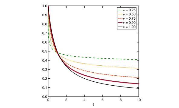
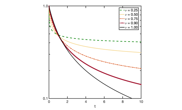
Figure 1. The composed function $E_{\nu,1}(-\ln^{\nu}(1+t))$ for $\nu=0.25,0.50,0.75,0.9,1$ in the time range $0\leq t\leq 10$.

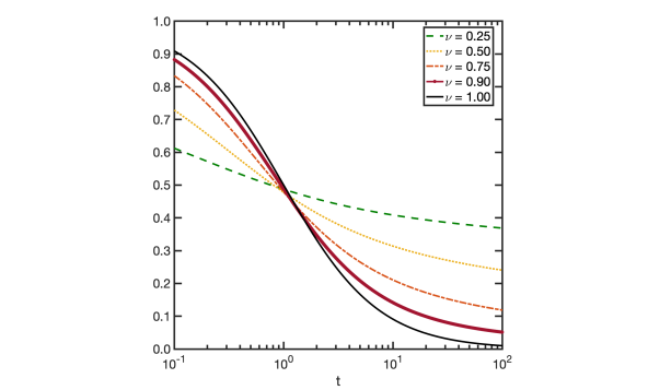
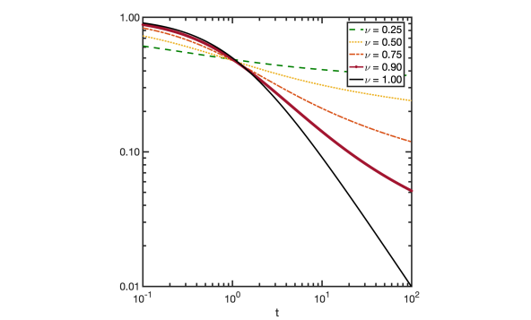
Figure 2. The composed function $E_{\nu,1}(-\ln^{\nu}(1+t))$ for $\nu=0.25,0.50,0.75,0.9,1$ in the time range $10^{-1}\leq t\leq 10^{+2}$.

The asymptotic representation for $t\to\infty$ of the function $E_{\nu,1}(-\ln^{\nu}(1+t))$ is readily obtained by the first term of the asymptotic series of the Mittag-Leffler function for $x>0$ and $\nu\in(0,1)$, see e.g [10]:

(3.5) $$E_{\nu,1}(-x)\sim-\sum_{n=1}^{\infty}\dfrac{(-1)^{n-1}\,x^{-n}}{\Gamma(1-\nu n)},\quad x\to\infty.$$

Then

(3.6) $$E_{\nu,1}(-\ln^{\nu}(1+t))\sim\dfrac{\ln^{-\nu}(1+t)}{\Gamma(1-\nu)},\quad t\to\infty.$$

so that we also try to find the matching with the above asymptotic representations as $t\to\infty$. We note that this matching is expected to be for very large values of time because the presence of the logarithm that is known to be a slow varying function. Of course in the limit $\nu\to 1^{-}$ we get a singular transition from a logarithmic decay to a power law decay because

(3.7) $$E_{1,1}(-\ln(1+t))=\exp(-\ln(1+t))=\dfrac{1}{1+t}\,,\quad t>0\,.$$

Then for this matching we add the case $\nu=0.95$ to point out the singular limit as $\nu$ is closer to 1.

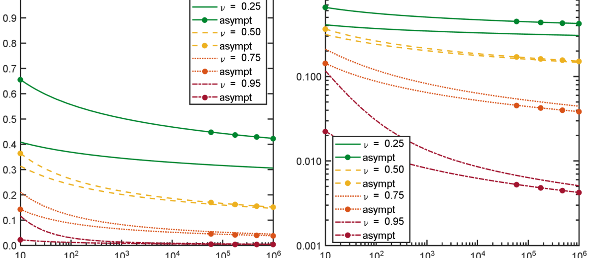
Figure 3. Plots in an enlarged logarithmic scale, compared with their asymptotic representations.

This can be understood in analogy with the singular limit of the classical Mittag-Leffler function $E_{\nu}(-x)$ of negative argument when $\nu\to 1^{-}$ as described in the recent paper by Paris [21] published in Fractional Calculus and Applied Analysis to which the interested reader is asked to refer. In Figure 3, we show the comparison between the plots in an enlarged logarithmic scale and their asymptotic representations. It is evident that the accurate value of the Mittag-Leffler function approaches the corresponding asymptotic representation with a good agreement.
Since the function $\ln^{\nu}(1+t)$ for $\nu\in(0,1)$ is a Bernstein function as in the case $\nu=1$, then the stress (3.3) is relaxing as a completely monotone function in analogy with standard fractional Maxwell model, see e.g.[15]. Indeed, we observe that this function can be obtained as the composition of the two Bernstein functions $x^{\nu}$ and $log(1+t)$, see e.g. the treatise by Schilling et al [23].

4. Conclusions

In this paper we consider an explorative mathematical modification of the fractional Maxwell model based on the application of Hadamard-type derivatives. It is well-known and widely accepted that time-fractional models in viscoelasticity have the advantage to take into account memory effects in relaxation processes. The main aim of this paper is to combine two different effects in a single theoretical model. Considering the recent studies about the role of time-dependent viscosity coefficient in the Maxwell model (see [20]), we here suggest to consider in a single operator memory-effects and time-dependent viscosity. This fractional operator results as a deterministic time-change from the Caputo derivative and the modified Maxwell model leads to an ultra-slow relaxation process. We underline that the relaxation response obtained in [20] can be recovered as a special case.
The idea to apply Hadamard-type derivatives in viscoelasticity is inspired by the recent studies for the formulation of a generalized Lomnitz creep law (see [7]). Moreover, different mathematical approaches for ultra-slow relaxation models are gaining interest and this topic is of relevant interest for the applications (we refer in particular to [13] and [24]). In our view the analysis of ultra-slow relaxation models based on the Hadamard-fractional calculus approach should be still deepened. From the theoretical point of view, Hadamard-type derivatives can be obtained as a particular choice of fractional derivatives w.r.t. another functions. Modified Maxwell models based on fractional derivatives w.r.t. another functions can be object of future interest in order to consider different time-dependence of the viscosity coefficients and leading to different relaxation response. A similar idea was recently considered for generalized Scott-Blair models in [6].
We finally observe that a similar model was considered in [14]. In comparison with this paper, we introduce the analysis of this model in the context of the literature, providing physical motivations and new graphical simulations.

References

- [1] Almeida, R., A Caputo fractional derivative of a function with respect to another function, Commun. Nonlinear Sci. Numer. Simulat. 44 (2017), 460–481.
- [2] Almeida, R., Jleli, M., Samet, B. (2019). A numerical study of fractional relaxation–oscillation equations involving -Caputo fractional derivative. Revista de la Real Academia de Ciencias Exactas, Físicas y Naturales. Serie A. Matemáticas, 113(3), 1873-1891.
- [3] Beghin, L., Garra, R., Macci, C., Correlated fractional counting processes on a finite-time interval. Journal of Applied Probability 52 No 4 (2015), 1045–1061. [E-print: arXiv:1407.6844v2 [math.PR]]
- [4] Chechkin, A. V., Klafter, J., Sokolov, I. M., Fractional Fokker-Planck equation for ultraslow kinetics, Europhysics Lett. 63 No 3 (2003), 326–332. [E-print: https://arxiv.org/pdf/cond-mat/0301487]
- [5] Chen, W., Liang, Y., Hei, X., Structural derivative based on inverse Mittag-Leffler function for modeling ultraslow diffusion, Fract. Calc. Appl. Anal. 19 No 5 (2016), 1250–1261. [DOI: 10.1515/fca-2016-0064]
- [6] Colombaro, I., Garra, R., Giusti, A., Mainardi, F. (2018). Scott-Blair models with time-varying viscosity. Applied Mathematics Letters, 86, 57-63.
- [7] Garra, R., Mainardi, F., Spada, G. (2017). A generalization of the Lomnitz logarithmic creep law via Hadamard fractional calculus. Chaos, Solitons & Fractals, 102, 333-338.
- [8] Garrappa, R., The Mittag-Leffler function in two and three parameters (ml.m code) 2014. WEB Site of MATLAB Central http://www.mathworks.com/matlabcentral/fileexchange
- [9] Garrappa, R., Numerical evaluation of two and three parameter Mittag-Leffler function, SIAM J. Numer. Anal. 53 No 3 (2015), 1350–1369. DOI:10.1137/140971191
- [10] Gorenflo, R., Kilbas, A.A., Mainardi, F., Rogosin, S.V., Mittag-Leffler Functions, Related Topics and Applications, 2-nd edition, Springer Verlag, Berlin (2020).
- [11] Kilbas, A.A., Srivastava, H.M., Trujillo, J.J., Theory and Applications of Fractional Differential Equations, Elsevier, Amsterdam (2006).
- [12] Lattanzi, A., Casasanta, G., Garra, R. (2022). On the application of Mittag–Leffler functions to hyperbolic-type decay of luminescence. Journal of Physics and Chemistry of Solids, 163, 110538.
- [13] Liang, Y., Yu, Y., Magin, R. L., Computation of the inverse Mittag–Leffler function and its application to modeling ultraslow dynamics. Fract. Calc. Appl. Anal., 25(2) (2022), 439-452, [DOI: https://doi.org/10.1007/s13540-022-00020-8]
- [14] Long, J., Xiao, R., Chen, W., Fractional viscoelastic models with non-singular kernels, Mechanics of Materials, 127 (2018): 55-64.
- [15] Mainardi, F., Fractional Calculus and Waves in Linear Viscoelasticity, 2-nd edition, World Scientific, Singapore (2022)
-
[16]
Mainardi, F., Mura, A., Gorenflo, R.,
Stojanovic, M.,
The two forms of fractional relaxation of distributed order,
J. Vibration and Control13 (2007), 1249–1268.
[E-print
tthttp://arxiv.org/abs/cond-mat/0701131] - [17] Mainardi, F., Mura, A., Pagnini, G., Gorenflo, R., Time-fractional diffusion of distributed order, J. Vibration and Control, 14 (2008), 1267–1290. [E-print http://arxiv.org/abs/cond-mat/0701132]
- [18] Mainardi, F., Spada, G. (2011). Creep, relaxation and viscosity properties for basic fractional models in rheology. European Physical Journal Special Topics, 193(1), 133-160.
- [19] Metzler, R., Klafter, J., The restaurant at the end of the random walk: Recent developments in the description of anomalous transport by fractional dynamics, J. Phys. A. Math. Gen. 37 (2004), R161–R208.
- [20] Pandey, V., Holm, S., Linking the fractional derivative and the Lomnitz creep law to non–Newtonian time–varying viscosity, Physical Review E 94 (2016), 032606/1-6.
- [21] Paris, R.B., Asymptotics of the Mittag-Leffler function on the negative real axis when . Fract. Calc. Appl. Anal. 25 (2022), 735–746, [DOI: https://doi.org/10.1007/s13540-022-00031-5]
- [22] Rekhviashvili, S. S., Pskhu, A. V. (2022). A Fractional Oscillator with an Exponential-Power Memory Function. Technical Physics Letters, 1-4.
- [23] Schilling, R.L., Song, R., Vondracek, Z., Bernstein Functions: Theory and Applications, De Gruyter (2012).
- [24] Su, X., Chen, W., Xu, W., Liang, Y. (2018). Non-local structural derivative Maxwell model for characterizing ultra-slow rheology in concrete. Construction and Building Materials, 190, 342-348.
- [25] Yang, X., Cai, W., Liang, Y., Holm, S. (2020). A novel representation of time-varying viscosity with power-law and comparative study. International Journal of Non-linear Mechanics, 119, 103372.