Correlation-based feature selection to identify functional dynamics in proteins

Abstract

To interpret molecular dynamics simulations of biomolecular systems, systematic dimensionality reduction methods are commonly employed. Among others, this includes principal component analysis (PCA) and time-lagged independent component analysis (TICA), which aim to maximize the variance and the timescale of the first components, respectively. A crucial first step of such an analysis is the identification of suitable and relevant input coordinates (the so-called features), such as backbone dihedral angles and interresidue distances. As typically only a small subset of those coordinates is involved in a specific biomolecular process, it is important to discard the remaining uncorrelated motions or weakly correlated noise coordinates. This is because they may exhibit large amplitudes or long timescales and therefore will be erroneously be considered important by PCA and TICA, respectively. To discriminate collective motions underlying functional dynamics from uncorrelated motions, the correlation matrix of the input coordinates is block-diagonalized by a clustering method. This strategy avoids possible bias due to presumed functional observables and conformational states or variation principles that maximize variance or timescales. Considering several linear and nonlinear correlation measures and various clustering algorithms, it is shown that the combination of linear correlation and the Leiden community detection algorithm yields excellent results for all considered model systems. These include the functional motion of T4 lysozyme to demonstrate the successful identification of collective motion, as well as the folding of villin headpiece to highlight the physical interpretation of the correlated motions in terms of a functional mechanism.

G. Diez and D. Nagel contributed equally to this work. G. Diez and D. Nagel contributed equally to this work.

1 Introduction

Molecular dynamics (MD) simulation is a versatile and widely used approach to study the spatiotemporal dynamics of biomolecular systems.¹ Since it is neither possible nor desirable to follow the motion of a complex molecule along its $3N$ atomic coordinates, a low-dimensional representation of the dynamics is required, which explains the mechanism and the underlying structural rearrangements of some biomolecular process. ^{2, 3, 4, 5, 6, 7} To this end, a number of efficient and systematic strategies of dimensionality reduction have been developed.^{8, 9} Popular examples include principal component analysis¹⁰ (PCA) which represents a linear transformation to coordinates that maximize the variance of the first components, and time-lagged independent component analysis¹¹ (TICA) which aims to maximize the timescales of the first components. Moreover a variety of nonlinear techniques as well as a rapidly increasing number of machine-learning empowered approaches have been proposed, see, e.g., Refs. 12, 13, 14 for reviews.

In this work, we are concerned with the crucial initial step in biomolecular dimensionality reduction, that is, the identification of suitable and relevant input coordinates for the analysis.¹⁵ First the type of coordinates needs to be chosen. Due to inevitable mixing of overall rotation and internal motion, Cartesian coordinates are in general not suited for dimensionality reduction.^{16, 17} Internal coordinates such as dihedral angles and interatomic distances, on the other hand, are by definition not plagued by this problem and also represent a natural choice, since the molecular force field is given in terms of internal coordinates. While $(\phi,\,\psi)$ backbone dihedral angles have been shown to accurately describe the conformation of secondary structures such as $\alpha$-helices and $\beta$-sheets, ^{18, 19} interresidue distances appear to be well suited to characterize the overall structure of a protein.^{20, 21, 22} A drawback of using interresidue distances is that their number scales quadratically with the number of residues. To avoid this overrepresentation, it has been suggested to restrict the analysis on distances reflecting interresidue contacts such as hydrogen bonds, salt bridges, and hydrophobic contacts.²³ In this way, we focus on near order effects rather than long distances, because the latter can be typically understood as a consequence of contact changes.

Irrespective of the type of input coordinates, we may expect that only a subset of them will be involved in a specific biomolecular process. A general approach to identify these relevant coordinates of a process is to consider their mutual relation, as quantified by some correlation measure.^{24, 25} For example, functional mode analysis^{26, 27} aims to identify molecular coordinates that significantly correlate with some pre-defined functional observable of the system, reflecting, e.g., the transition from an active to an inactive conformational state. This strategy excludes coordinates that do not change during the functional motion (e.g., stable contacts), as well as coordinates that change randomly such as wildly dangling terminal residues. Exclusion of the latter is particularly important if we intend to subsequently perform a PCA. Maximizing the variance of the first principal components, PCA would rate this terminal large-amplitude motion as important, although it is generally irrelevant for protein function. Maximizing the timescales of the first components, a similar problem occurs for TICA if the coordinates contain slow but irrelevant motions.²⁸ For example, when performing TICA on $(\phi,\,\psi)$ dihedral angles to describe the folding of the helical protein HP35,¹⁵ it correctly identifies transitions between right- and left-handed helices as slowest process.²⁹ Since the left-handed helices are hardly populated, however, this motion is not relevant for the folding process and the corresponding deceptive coordinates should therefore be discarded in the further analysis.¹⁵

Here we wish to identify coordinates, often called “features”, which describe motions that are involved in a specific process, and thus discard the remaining coordinates from the analysis, describing other processes and random motion or noise. Due to the reduction of noise and its lower dimensionality, the resulting feature space considerably facilitates the subsequent analysis and may even lead to a straightforward interpretation of the considered process. As we aim to perform the feature selection in an unbiased manner, we avoid variation principles that maximize variance or timescales.³⁰ Moreover, we do not want to invoke previously known functional observables as in functional mode analysis ²⁶ or refer to pre-defined metastable conformational states as in a recently proposed supervised machine learning scheme.³¹ Rather, we follow the strategy pursued by Tiwary and coworkers³² and first calculate the correlation matrix of all input coordinates to establish their interrelation, and then block-diagonalize this matrix to unravel which set of coordinates is associated with the process under consideration. A somewhat related approach is followed by various groups that aim to construct a dynamical network of protein residues in order to map out pathways of allosteric communication.^{33, 34, 35, 36} Representing the features as data points in a similarity space where the features are arranged according to their proximity, the latter step can be viewed as a straightforward clustering task which identifies groups of nearby data points. Numerous options exist to achieve this clustering,³⁷ including hierarchical methods (such as complete linkage clustering³⁸), geometrical approaches (such as $k$-medoids³⁹) or graph-based community detection methods.^{40, 41}

In this work we introduce the Python package MoSAIC (“Molecular Systems Automated Identification of Cooperativity”), which automatically detects collective motions in MD simulation data, identifies uncorrelated coordinates as noise, and hence provides a detailed picture of the key coordinates driving a conformational change in a biomolecular system. Considering several linear and nonlinear correlation measures and various clustering algorithms, we show that the combination of linear correlation and the Leiden community detection algorithm ⁴² yields excellent results for all considered model systems. These include a model correlation matrix with known ground truth to test various clustering approaches, the functional motion of T4 lysozyme ⁴³ to demonstrate the successful identification of collective motion, as well as the folding of villin headpiece ⁴⁴ to highlight the physical interpretation of the resulting clusters in terms of a functional mechanism.

2 Correlation Measures

In order to establish a suitable similarity measure to identify collective motion in proteins, we introduce various definitions of the correlation and study their performance for our set of model problems.

2.1 Linear and nonlinear correlation

Given two random variables $X$ and $Y$, the linear correlation $\rho$ is defined as the Pearson correlation coefficient

$$\rho(X,Y)=\frac{\langle(X-\langle X\rangle)(Y-\langle Y\rangle)\rangle}{\sigma_{X}\sigma_{Y}}\,,$$ (1)

where $\langle\ldots\rangle$ denotes the statistical average and $\sigma$ is the standard deviation. $\rho$ ranges from $-1$ to $1$, where a value of $0$ implies no linear correlation at all while values of $\pm 1$ corresponds to a perfect linear relationship between $X$ and $Y$. In that case, one variable can be fully described by the other variable, and may therefore be discarded if we are interested in dimensionality reduction. By definition, the Pearson coefficient considers only the first two moments of the underlying distribution, which—strictly speaking—is adequate only for normally distributed data. From a Physics point of view, this translates into a quadratic energy landscape associated with a linear force.¹

To go beyond the linear regime, we consider the mutual information $I(X,Y)$ of two variables, which can be defined as ⁴⁵

$$I(X,Y) =H(X)-H(X|Y)\,,$$ (2)

$$H(X) =-\sum_{x\in X}p(x)\log p(x)\,,$$ (3)

where $H(X)$ is the information entropy that measures the uncertainty of a discrete random variable $X$ with samples $x$, $H(X|Y)$ is the corresponding conditional entropy, and $p(x)$ denotes the probability distribution of $X$. Since $H(X)$ can be viewed as the uncertainty about $X$, $H(X|Y)$ may be interpreted as the uncertainty about $X$ remaining after knowing $Y$, i.e., it indicates what $Y$ does not tell us about $X$. Consequently, mutual information can be viewed as the reduction in uncertainty of $X$ due to the knowledge of $Y$, thus offering a theoretically well justified measure of how similar two random variables are. Alternatively, the mutual information can be defined as measure of statistical independence of variables $X$ and $Y$, i.e., the discrepancy between the joint distribution $p(x,y)$ and the product of the marginal distributions $p(x)p(y)$. Employing the Kullback-Leibler divergence $D_{\text{KL}}\left[p_{1}||p_{2}\right]$ as a commonly used measure for the dissimilarity of two probability distributions $p_{1}$ and $p_{2}$, we obtain

$$I(X,Y) =D_{\text{KL}}\left[p(x,y)||p(x)p(y)\right]$$

$$=\sum_{x\in X}\sum_{y\in Y}p(x,y)\log_{2}\left[\frac{p(x,y)}{p(x)p(y)}\right]\,.$$ (4)

Being defined via probability distributions that contain all statistical moments, the mutual information is not restricted to linear correlation as the Pearson correlation coefficient in Eq. (1). On the other hand, the mutual information is not bound to $[-1,1]$ but ranges from $[0,\infty)$, which is a drawback, as it is not obvious which range of the mutual information can be considered as high or low correlation. To this end, several options are at hand to normalize the mutual information. ⁴⁶ Employing the inequality

$$I(X,Y)\leq\sqrt{H(X)H(Y)}\leq H(X,Y)\,,$$ (5)

we may adopt the geometric mean of marginal entropies $\sqrt{H(X)H(Y)}$ or the joint entropy $H(X,Y)$ to define the normalized quantities

$$I_{\text{geom.}}(X,Y) =\frac{I(X,Y)}{\sqrt{H(X)H(Y)}}\,,$$ (6)

$$I_{\text{joint}}(X,Y) =\frac{I(X,Y)}{H(X,Y)}\,.$$ (7)

Alternatively, we can use the Jensen-Shannon divergence $D_{\textsc{js}}$ as a similarity measure of $p(x,y)$ and $p(x)p(y)$, which by design it is bound to $[0,1]$. This leads to

$$I_{\textsc{js}}(X,Y)=D_{\textsc{js}}\left[p(x,y)||p(x)p(y)\right]$$ (8)

$$\quad=\frac{1}{2}D_{\textsc{kl}}\left[p(x,y)||M\right]+\frac{1}{2}D_{\textsc{kl}}\left[p(x)p(y)||M\right]$$ (9)

with $M=\frac{1}{2}\left[p(x,y)+p(x)p(y)\right]$. As a final option we mention the formulation of Gel’fand and Yaglom, ⁴⁷ who showed that in the special case that the joint probability distribution $p(x,y)$ is a bivariate normal distribution, the mutual information $I$ can be deduced exactly from linear correlation $\rho$ via

$$I(X,Y) =-\frac{1}{2}\log[1-\rho(X,Y)^{2}]\,.$$ (10)

The identity can be used to normalize the mutual information by solving for $\rho$ and defining

$$I_{\textsc{gy}}(X,Y)\equiv\rho(X,Y) =\sqrt{1-\exp\left[-2I(X,Y)\right]}\,,$$ (11)

which corresponds to a transformation of the mutual information to a linear correlation.

While the linear correlation in Eq. (1) is readily calculated, the computation of the mutual information is significantly more involved, because it requires the estimation of (at least) two-dimensional probability distributions. Apart from a simple histogram ansatz, which converges slowly (with respect to the sample size) and is not very robust, ⁴⁸ we may employ a kernel density estimation, which is numerically expensive and requires the selection of a bandwidth parameter,⁴⁹ or a non-parametric $k$-nearest neighbor ($k$-nn) density estimator,⁵⁰ which is computationally expensive as well. Comparing the three methods, kernel density and $k$-nn estimators are found to converge faster (with respect to the sample size) than the histogram estimator, but also require factors 100 and 10 more CPU time, respectively (see Fig. S1a,b). Compared to calculation of the linear correlation, the reliable estimation of the mutual information requires at least a factor $\sim 10^{3}$ more computation time (Fig. S1c).

2.2 Choice of similarity measure

To assess the performance of the above introduced correlation measures, we calculated for each measure correlation matrices obtained from the MD simulations of our model proteins HP35 and T4L (see Sec. 4). As the results are quite similar for both systems (Fig. S3), in the following we combined these data to facilitate the discussion. To get a first impression of the overall difference between linear and nonlinear correlations, Fig. 1a compares the results obtained for the absolute Pearson coefficient $|\rho|$ and $I_{\text{geom.}}$, the mutual information normalized by its tightest bound according to Eq. (5). Remarkably, the resulting contour plot reveals a clear relation between the two correlation measures. Quite similar results are found for the other normalizations of the mutual information (Fig. S3). This appears to indicate that the nonlinear measures do not contain significant additional information compared to the linear correlation.

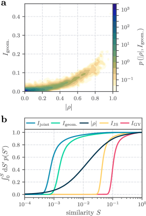
Figure 1: Comparison of linear and nonlinear correlation measures, obtained from MD data of all protein systems. (a) Mutual information normalized by the geometric mean, $I_{\text{geom.}}$, compared to the absolute Pearson coefficient $|\rho|$. (b) Cumulative probability distribution of various similarity measures.

While the values for $|\rho|$ cover the full range from $0$ to $1$, the values for $I_{\text{geom.}}$ hardly exceed values of $0.2$. To further illustrate this effect, Fig. 1b depicts the cumulative probability distribution of $I_{\text{geom.}}$, showing that more than $90\text{\,}\%$ of the taken values lie below $0.01$. Considering the other nonlinear measures, we find that $I_{\text{joint}}$ behaves quite similar, while $I_{\textsc{JS}}$ and $I_{\textsc{GY}}$ adopt mainly high values and hardly show values below $I_{\text{JS}}=0.03$ or $I_{\textsc{GY}}=0.07$, respectively. That is, although all nonlinear measures are based on the same mutual information [Eq. (4)], we hardly find an overlap between the probability distributions of the various normalized quantities. The linear correlation $|\rho|$, on the other hand, is found to uniformly account for small and high correlations. Combined with the result of Fig. 1a that the mutual information does not seem to provide essential new information and the considerably higher ($\gtrsim 10^{3}$ times) numerical effort (Fig. S1c), the above findings clearly suggest the simple and well-established linear Pearson coefficient as suitable similarity measure.

As a note of caution, we mention that the Pearson coefficient $\rho$ may have serious flaws, in particular, if vector-valued data are considered.⁵¹ A well-known example is data lying on a circle centered around the origin, for which $\rho$ is zero despite the perfectly correlated data. Restricting ourselves to scalar data, on the other hand, the Pearson coefficient is known to capture the overall correlation quite well.²⁴ Collinear data in particular includes distances, but also periodic variables (such as angles and dihedral angles) if an appropriate transformation to linear variables is applied.^{52, 53} That is, the linear correlation measure should be sufficient for internal molecular coordinates, but may be problematic for Cartesian coordinates.³⁴ Moreover we note that the considerable similarity between linear and nonlinear correlation is somewhat surprising, because the Pearson coefficient considers only the first two moments of the underlying distribution [Eq. (1)] and the probability distributions of the employed MD data are not necessarily normally distributed. For example, we consider contact distances for HP35 and T4L, which typically reveal a prominent peak at small distances (reflecting the bound state), and a flat distribution at large distances indicating unbound conformations. Nevertheless, the resulting differences between linear and nonlinear correlations were found to be minor.

3 Community detection of collective motion

Having established a similarity measure to quantify the correlation between coordinates, we aim to block-diagonalize the resulting correlation matrix in order to identify the coordinates involved in some cooperative motion. As discussed in the Introduction, numerous approaches and algorithms exist for this type of clustering task. ³⁷ For the specific application (complex motions of biomolecules) considered here, we show below that the Leiden community detection algorithm developed by Traag et al.⁴² appears favorable.

For the further discussion, though, it is instructive to first briefly introduce two standard methods, $k$-medoids³⁹ and complete linkage clustering.³⁸ $k$-medoids is a classical partition technique and bears many similarities with the popular $k$-means algorithm.⁵⁴ Given a set of data points and dissimilarity among them (which we can directly compute as $1-|\rho|$), the approach initializes $k$ data points as medoids and assigns each data point to the nearest medoid. Then the medoids are greedily optimized (i.e., relying on locally optimal decisions) until the dissimilarity of all points belonging to a cluster and the designated medoid (i.e., the center of the cluster) is minimized. The number of clusters $k$ must be chosen a priori and therefore does not represent an intrinsic property of the system.

Complete linkage clustering is an agglomerative hierarchical clustering method which combines data points sequentially into larger clusters.³⁸ While initially each data point represents its own cluster, at each step of the algorithm the clusters separated by the shortest distance are merged. In case the clusters contain more than a single data point, the distance between clusters is regarded as the maximum distance between any two elements of the two clusters. Repeating this step multiple times and merging the closest clusters together in each step, we eventually end up with a single cluster. To illustrates the sequence of merging clusters, the process can be visualized as a dendrogram. By choosing some cutoff-value in this dendrogram, we obtain the final clustering.

3.1 Clustering: The Leiden algorithm

In contrast to $k$-medoids or complete linkage clustering, the Leiden algorithm⁴² is performed on a graph, i.e., we need to represent the correlation matrix in terms of nodes and edges. Here each node describes a coordinate of the system and the edges between the nodes describe how similar (i.e., correlated) they are. Based on such a graph, the Leiden algorithm identifies communities of similar coordinates by unraveling the graph’s cluster structure through a maximization of an objective function (see below). The procedure represents an improvement of the popular Louvain algorithm,⁵⁵ as it introduces randomness in the selection of the community assignment, which facilitates a global optimal partitioning by exploring the partition space more broadly. (See the supplementary information in Ref. 42 for a detailed description.) Roughly speaking, the algorithm consists of three steps that are performed iteratively until the objective function is not more improved. (1) The nodes are moved to the communities that yield the highest gain of the objective function. (2) To improve the quality of the partitioning, the communities of step 1 may be split into multiple subcommunities. (3) The (sub)communities of step 2 now become nodes, thus achieving a coarse graining of the graph.

A widely-used objective function $\Phi$ in community detection is modularity, which indicates the amount of cluster-like structures in a graph.⁵⁶ That is, high values of modularity suggest that dense communities of nodes exist, which strongly interact internally but are only loosely connected to the rest of the graph. Low values, on the other hand, indicate that the graph shows only little order but may be regarded as randomly wired network. Modularity can be defined as

$$\Phi_{\text{mod}}=\frac{1}{2m}\sum_{c}\left(e_{c}-\frac{k^{2}_{c}}{2m}\right)\,,$$ (12)

where the sum runs over all clusters $c$, $m$ denotes the total number of edges in the graph, $e_{c}$ is the sum of edge weights within cluster $c$, and $k_{c}$ represents the sum of the degrees (i.e., number of connecting edges) of all nodes in $c$. While the first term favors the formation of large clusters, the penalty term $k_{c}^{2}/2m$ prevents the clusters from becoming too large, as it represents the expected numbers of edges within each cluster in a randomly rewired graph, where the number of nodes are identical, and all nodes keep their degree. However, this implies that every node can be connected to every other node, which is very unlikely in large graphs, since the vicinity of each node only covers a small part of the graph. Moreover, the expected number of edges in such large graphs become very small (in the order of $N^{-1}$, where $N$ denotes the number of nodes in the graph), which is why even a single link between small communities might be interpreted as a sign of strong correlation that may cause the merging of the communities independently of their features. Therefore, if the graph is large enough, this implies that two perfectly homogeneous clusters that represent completely different collective motions would be merged at some point. Ultimately this issue represents a resolution limit for the identification of small clusters in large graphs.⁵⁷

To circumvent this problem, Traag et al.⁵⁸ introduced a new objective function, referred to as “constant Potts model” (CPM). As for modularity, CPM can be derived from the Potts model,⁵⁹ which is a generalization of the Ising model. The objective function reads

$$\Phi_{\textsc{cpm}}=\sum_{c}\left[e_{c}-\gamma\binom{n_{c}}{2}\right]\,,$$ (13)

where $n_{c}$ denotes the number of nodes in cluster $c$ and the binomial $\binom{n_{c}}{2}=(n_{c}^{2}-n_{c})/2$ represents the number of possible edges within $c$. Weighting this number by the resolution parameter $\gamma$, Eq. (13) compares the sum of edges in cluster $c$ (i.e., the total correlation within $c$) to the edge sum of a cluster of the same size but with all coordinates being $\gamma$-correlated. If cluster $c$ performs better, it contributes positively, otherwise the partitioning is penalized. In this way, $\gamma$ determines the minimal average correlation required within clusters. We note, however, that individual correlations can also be below $\gamma$ if the overall function benefits from it, which is in fact an important advantage over methods like complete linkage clustering. Hence, the resolution parameter $\gamma$ controls the coarseness of the clustering: A high $\gamma$-value and therefore a high resolution leads to many communities, while lower resolution means less, but also larger and thus more heterogeneous communities.

3.2 Optimal Clustering Strategy

To compare the different clustering approaches introduced above, we constructed as benchmark problem an artificial correlation matrix that mimics the correlations found in protein systems. Inspired by our results on HP35 and T4L below, we opted for a model that features three larger clusters (containing various correlated coordinates) and multiple mini-clusters reflecting noise coordinates. As a challenge, we also included small residual correlations between the clusters (see SI Methods). Figure 2 compares the resulting block-diagonal correlation matrix to the outcome of the following clustering methods, which were applied to the matrix with a random order of coordinates: $k$-medoids, complete linkage and the Leiden algorithm using modularity or CPM as objective function. To facilitate an unbiased comparison, we spend some effort to optimize the parameters of each method. That is, we used the silhouette method⁶⁰ to find initial estimates, and determined the optimal value of the parameters via V-measure⁶¹ which compares the clustering to the reference results (Fig. S2). This is relatively straightforward for complete linkage and Leiden/CPM clustering that only require an evident resolution parameter, but less so for $k$-medoids and Leiden/modularity.

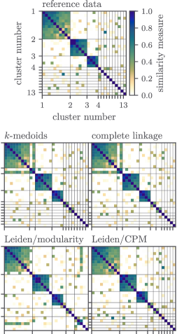
Figure 2: Simple model of a correlation matrix, consisting of three clusters of size 10, 6, and 4, as well as of 10 noise coordinates. Reference results are compared to the clustering methods $k$-medoids, complete linkage and the Leiden algorithm using modularity and CPM as objective functions.

While all methods shown in Fig. 2 reproduce the overall picture of main clusters and noise coordinates, they differ in several possibly important aspects. That is, to successfully identify collective protein motions, a clustering scheme should fulfill the following requirements:

1. Completeness: All coordinates corresponding to a specific collective motion should be assigned to a single cluster. As a consequence, each cluster completely accounts for a specific collective motion.

2. Homogeneity: Each cluster should exclusively contain features which represent the same collective motion.⁶¹ This ensures that the clusters are as small as possible, such that noise coordinates can be reliably identified.

In the light of these criteria, we notice that all algorithms except Leiden/CPM do not satisfy the completeness criteria. For example, they fail to correctly define cluster 1, which shows relatively strong correlation to noise coordinates. Showing sporadic correlation with coordinates that describe collective motion, noise coordinates can lead to the formation of a new cluster, thus impeding the completeness of larger clusters describing collective motion. This is particularly an issue for $k$-medoids and complete linkage clustering, which rely on greedy decision-making. The Leiden algorithm using modularity is plagued by similar problems, because it is based on a $k$-nearest neighbor graph that focuses on the local neighborhood.⁵⁷ As discussed above, modularity effectively introduces a resolution limit for small clusters, which hampers the resolution of the noise coordinates in Fig. 2.

On the other hand, the Leiden algorithm combined with CPM, henceforth referred to as “Leiden clustering”, is able to obtain complete clusters by permitting of locally suboptimal decisions, which facilitate to find the global maximum of the objective function. Moreover, the approach only requires to determine the single intuitive resolution parameter $\gamma$. While these virtues of the Leiden clustering may have only a small effect in Fig. 2, they are shown to result in significant differences for the protein models studied below.

4 Applications

We are now in a position to apply the above established strategy (i.e., Leiden clustering of the linear correlation matrix) to identify collective motions and the underlying functional mechanism of selected protein systems. We start with the characterization of the cooperative open-closed motion of T4 lysozyme⁴³ (T4L), which demonstrates the capability of Leiden clustering to distinguish functional coordinates from noise. Studying the folding of villin headpiece (HP35), we show that Leiden clusters can be a valuable means to characterize the folding pathways of the system. All correlation measures and clustering methods introduced above are implemented in the Python package MoSAIC (“Molecular Systems Automated Identification of Cooperativity”), which adapts the scikit-learn syntax⁶² and is available on our homepage.⁶³

4.1 Functional Dynamics of T4 Lysozyme

T4L is a 164-residue enzyme that performs an open-closed transition of its two domains, which is triggered by local motions in the hinge region⁴³ (Fig. 3a). While the lifetimes of the open and closed state are in the order of a few microseconds, the transitions between these states occur on a nanosecond timescale, thus indicating cooperative behavior. As discussed in previous work, ^{26, 43, 31} the identification of reaction coordinates underlying this cooperative process poses a challenge to standard dimensionality reduction approaches. Here we adopt the $50\text{\,}\mathrm{\SIUnitSymbolMicro s}$-long all-atom MD simulation by Ernst et al.,⁴³ which was carried out using Gromacs 4.6.7 (Ref. 64), the Amber ff99SB*-ILDN force field ^{65, 66, 67} and the TIP3P water model.⁶⁸ Assuming that a contact is formed if the distance $d_{ij}$ between the closest non-hydrogen atoms of residues $i$ and $j$ is shorter than $4.5\text{\,}\mathrm{\SIUnitSymbolAngstrom}$ (Ref. 23), $402$ native interresidue contacts were identified,⁴³ and the associated contact distances $d_{ij}$ were used to calculate the linear correlation matrix.

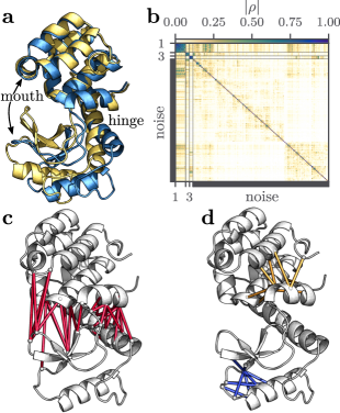
Figure 3: (a) Structure of the open (blue) and closed (yellow) states of T4L. The arrow indicates the Pac-Man-like open-closed transition of the mouth region, which is triggered by local motions in the hinge region. (b) Block-diagonalized correlation matrix of T4L, discriminating three clusters describing correlated motion from numerous noise coordinates. (c) Illustration of the interresidue contacts (red lines) contained in cluster 1 of the Leiden clustering, mediating the allosteric coupling between the distant mouth and hinge regions. (d) Interresidue contacts pertaining to cluster 2 (yellow) and cluster 3 (blue).

When we perform Leiden clustering using a resolution parameter of $\gamma=0.5$ and assigning clusters containing $5$ or less coordinates to noise, we obtain the block-diagonalized correlation matrix shown in Fig. 3b. Interestingly, we find only three main clusters representing correlated motion, while the majority of coordinates are hardly correlated and thus distributed over the remaining $\sim 300$ clusters. To be specific, this means that the average correlation within the main clusters is $\langle|\rho|\rangle=0.688$, while the mean residual correlation between the three main clusters is $0.085$, and the residual correlation between any two clusters (including the noise clusters) is on average only $0.035$. This is because most intraprotein contacts of T4L are quite stable and only fluctuate around their mean distance, while contacts on the protein surface frequently form and break and hence fluctuate randomly. In effect, all these coordinates represent noise that should be discarded in a further analysis. We note that the other clustering methods introduced above either fail to accurately recognize the noise coordinates ($k$-medoids and Leiden/modularity) or to properly identify the three main clusters ($k$-medoids and complete linkage), see Fig. S4.

Having discarded the noise, we now turn to the first three clusters that account for specific correlated motions of the system. In particular, the 27 highly correlated contact distances of cluster 1 are found to describe the functional open-closed transition of T4L. This is illustrated in Fig. 3c, which shows that these distances span the space connecting the mouth and hinge regions, and therefore reflect the allosteric coupling between these two distant regions.⁶⁹ Largely uncorrelated to cluster 1, clusters 2 and 3 account for other correlated motions of T4L. As shown in Fig. 3d, cluster 2 describes a rocking motion involving the rearrangement of $\alpha_{1}$ and the N-terminal domain, while cluster 3 contains a twist-like motion of the $\beta$-sheets and the close-by $\alpha_{2}$-helix. That is, Leiden clustering is able to discriminate several independent processes that occur at the same time. These motions were previously found in higher principal components of various PCAs,^{26, 43} and were therefore discussed as a part of the functional dynamics. Being (almost) uncorrelated and thus not involved in the open-closed transition of T4L, however, these coordinates should not be included in the analysis of the open-closed mechanism. Having said that, we note that in dynamical network theory of allosteric communication, small residual correlations between highly connected communities can nevertheless describe interactions between several sub-processes of a protein. ^{33, 34, 35, 36}

4.2 Folding of Villin Headpiece

HP35 is a 35-residues protein fragment that represents a popular model of ultrafast protein folding.⁷⁰ It consists of a hydrophobic core with three helices (residues 3–10, 14–19, and 22–32) that are connected via two unstructured loops, see Fig. 4. Here we adopt a $\approx$300\text{\,}\mathrm{\SIUnitSymbolMicro s}$$ long all-atom MD trajectory of the fast folding Nle/Nle mutant at $360\text{\,}\mathrm{K}$ of Piana et al.,⁴⁴ which reveals about thirty folding events. Following Ref. 23, we use the 53 native contacts of the crystal structure⁷¹ (PDB 2f4k) to construct the correlation matrix. Leiden clustering using a resolution parameter of $\gamma=0.65$ yields the block-diagonal matrix shown in Fig. 4a. It reveals 7 highly correlated main clusters, the approximately overall uncorrelated cluster 8, and 10 weakly correlated small clusters that are recognized as noise coordinates. Although beeing divers in the partition of main and weakly correlated clusters, the other clustering methods introduced above produce roughly similar results, see Fig. S5a.

To provide an intuitive picture of the Leiden partitioning of the correlation matrix, Fig. 4b displays the individual contact distances associated with the main clusters. First off, we see that the coordinates of cluster 8 account for the motions of the N-terminus relative to the $\alpha_{1}$-helix, which are completely uncorrelated to the rest of the protein. As explained in the Introduction, it is important to exclude such uncorrelated terminal motion from the analysis. Dangling terminal residues may undergo large-amplitude motion that is consequently recognized in the first components of a PCA, although they are clearly not relevant for folding. A related problem occurs if the uncorrelated motion exhibits two-state behavior and performs transitions, e.g., between two orientations of the terminus. As a consequence, the resulting number of conformational states of the total system doubles trivially, which unnecessarily complicates the analysis. As in the case of T4L, we thus find that the identification and rejection of uncorrelated motions or weakly correlated noise coordinates represents a crucial initial step of a successful analysis.

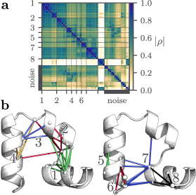
Figure 4: (a) Block-diagonalized correlation matrix of HP35, revealing seven main clusters, the overall uncorrelated cluster 8, and various noise coordinates. (b) Structure of HP35, indicating the contact distances included in clusters 1 to 8.

Apart from the reduction of the dimension of the problem, Leiden clustering may also support the interpretation of a considered biomolecular process. To this end, we consider clusters 1 to 7, which by design show high intracluster correlations ($\langle|\rho|\rangle=0.818$), but also significant residual correlations between the clusters (0.500 for main clusters only, 0.396 for all clusters), see Fig. 4a. Importantly, these intercluster correlations indicate that all seven clusters describe different aspects of the overall folding process. This is in contrast to the findings for T4L, where the main clusters are almost uncorrelated and thus describe independent processes.

With the exception of the small clusters 5 and (in part) 6 that account for motions within a helix, the main clusters of HP35 consist of tertiary contacts connecting two secondary structures (Fig. 4b). For example, cluster 1 connects helices $\alpha_{1}$ and $\alpha_{2}$, cluster 2 describes mostly correlations between the loops $\alpha_{1}$-$\alpha_{2}$ and $\alpha_{2}$-$\alpha_{3}$, and cluster 7 connects the helices $\alpha_{3}$ and $\alpha_{1}$. Due to high intracluster correlations, these contacts will preferably form and brake in a concerted manner, such that we may assign a state “1” to a cluster if (most) of its contacts are formed, and a state “0” if not. Describing the complete protein by a product state [e.g., (1110000) would mean that the contacts of the first three clusters are formed, the others not], we can characterize the structures of the folding trajectory in terms of this highly coarse grained state description.⁷² Since the clusters mostly refer to tertiary contacts, this state partitioning is in contrast to a state definition via helicity where, e.g., (ffu) means that the first two helices are folded and the helix 3 not.²⁹

As a simple application of the above idea, we may ask which clusters form first and which ones last in a successful folding event. By analyzing the MD trajectory, we find that clusters 3 and 4 that stabilize the connection of helices $\alpha_{1}$ and $\alpha_{2}$ typically fold first (Fig. S5c). Most interestingly, we learn that cluster 7 connecting the helices $\alpha_{3}$ and $\alpha_{1}$ forms last, and therefore represent the crucial step defining the transition state of the folding process. The example demonstrates that the coordinates defining the main clusters may give interesting first hints on the mechanism of the considered process.

5 Concluding remarks

We have introduced a correlation analysis method for MD simulation data, which aims to identify collective motions underlying functional dynamics. Given some input coordinates such as interresidue distances or backbone dihedral angles, the idea is to block-diagonalize the corresponding correlation matrix and subsequently associate the resulting clusters with functional motions or uncorrelated noise. Notably, this strategy avoids possible bias due to presumed functional observables²⁶ and conformational states³¹ or variation principles that maximize timescales.³⁰

To find the optimal algorithms for this workflow, we have considered several linear and nonlinear correlation measures and various clustering algorithms, which were implemented for a simple and scalable use in the Python package MoSAIC.⁶³ Interestingly, we have found that—at least for the considered systems—the simple and well-established Pearson coefficient describing linear correlation represents the best choice for this purpose. This is because all considered nonlinear measures (i.e., various versions of a normalized mutual information) do not provide essential new information (Fig. 1a), while they focus either on low or high values of the correlation (Fig. 1b) and require considerably higher ($\gtrsim 10^{3}$ times) numerical effort (Fig. S1c). Considering various clustering methods for matrix block-diagonalization, we have shown that the Leiden community detection algorithm⁴² performs best for all considered model systems. That is, Leiden clustering produces complete and homogeneous clusters that can be clearly assigned to correlated motions or noise (Fig. 2).

Adopting the open-closed transition of T4L and the folding of HP35 as representative examples, we have demonstrated the capability of Leiden clustering to discriminate cooperative functional dynamics from uncorrelated motions. In the case of T4L, $89\text{\,}\%$ of the 402 contact coordinates were assigned to noise, which reflects the fact that these contacts are either stable or fluctuate randomly (Fig. 3). In the case of HP35, we found several highly correlated main clusters, a large overall uncorrelated cluster, and various weakly correlated small clusters that were recognized as noise (Fig. 4). Reflecting large-amplitude motions of the N-terminus, the uncorrelated coordinates should be excluded from the analysis. This is because they may be rated as important by dimensionality reduction methods that maximize the variance (such as PCA), although they are clearly not relevant for folding. Performing Leiden clustering on the backbone dihedral angles of HP35, we are similarly led to exclude the uncorrelated motions of most of the $\phi$ angles, which (being slow but irrelevant) cause a breakdown of TICA.¹⁵ Hence, we find that the identification and rejection of uncorrelated motions or weakly correlated noise coordinates represents a crucial initial step of a successful dynamical analysis.

Apart from being a versatile feature selection scheme, Leiden clustering may also facilitate a simple interpretation of the considered biomolecular process. In the case of HP35, we obtained seven main clusters that are directly associated with tertiary contacts connecting secondary structures (Fig. 4). As contacts of a cluster by design form and brake in a concerted manner, we can employ the clusters as a coarse-grained state model to describe the folding process.⁷² Considering the time evolution of the clusters, for example, the model can be employed to illustrate the folding pathways of the HP35. In the case of T4L, Leiden clustering found three main clusters that account for specific correlated motions of the system (Fig. 3). While the 27 highly correlated contact distances of the first cluster describe the functional open-closed of T4L, the other two clusters account for other correlated motions of T4L and should therefore not be included in the analysis.

Various extensions of the above correlation analysis are currently under consideration. Following Tiwary and coworkers,³² for example, we aim to develop means to pick a few representative coordinates from each cluster, in order to achieve a small number of features describing the complete motion of a protein. Here, Leiden clustering using the constant Potts model is particularly advantageous, as we can simply control the extent of the coarse-graining by setting the resolution parameter. While we are generally reluctant to use Cartesian input coordinates (apart from the separation problem¹⁶, the computation of the correlation between non-scalar variables is notoriously difficult ²⁴), it would be nevertheless interesting to compare the outcomes of correlation analysis using contact distances and Cartesian $\text{C}_{\alpha}$ coordinates. This is because they account differently for non-trivial long-distance correlations, which are essential to understand allostery in proteins. ⁷³ Although numerous network models exist which aim to predict allosteric pathways, ^{33, 34, 35, 36} the results obtained from various formulations were found to differ significantly even for simple model proteins such as PDZ domains.⁷⁴

The authors thank Matthias Post, Steffen Wolf, Sofia Sartore and Marius Lange for fruitful discussions, and D. E. Shaw Research for sharing their trajectory of HP35. This work has been supported by the Deutsche Forschungsgemeinschaft (DFG) via the Research Unit FOR 5099 “Reducing complexity of nonequilibrium” (project No. 431945604). The authors acknowledge support by the bwUniCluster computing initiative, the High Performance and Cloud Computing Group at the Zentrum für Datenverarbeitung of the University of Tübingen, the state of Baden-Württemberg through bwHPC and the DFG through grant No. INST 37/935-1 FUGG.

The supplementary material contains details on the estimation of the mutual information, the optimization of clustering parameters, a comparison of different correlation measures and a comparison of T4L and HP35 using all clustering methods discussed in the paper.

All discussed correlation measures and clustering methods are implemented and freely available in the open-source software MoSAIC at github.com/moldyn.

References

- Berendsen 2007 Berendsen, H. J. C. Simulating the Physical World; Cambridge University Press: Cambridge, 2007
- Bolhuis et al. 2000 Bolhuis, P. G.; Dellago, C.; Chandler, D. Reaction coordinates of biomolecular isomerization. Proc. Natl. Acad. Sci. USA 2000, 97, 5877 – 5882
- Faradjian and Elber 2004 Faradjian, A. K.; Elber, R. Computing time scales from reaction coordinates by milestoning. J. Chem. Phys. 2004, 120, 10880–10889
- Best and Hummer 2005 Best, R. B.; Hummer, G. Reaction coordinates and rates from transition paths. Proc. Natl. Acad. Sci. USA 2005, 102, 6732–6737
- Krivov and Karplus 2008 Krivov, S. V.; Karplus, M. Diffusive reaction dynamics on invariant free energy profiles. Proc. Natl. Acad. Sci. USA 2008, 105, 13841 – 13846
- E and Vanden-Eijnden 2010 E, W.; Vanden-Eijnden, E. Transition-Path Theory and Path-Finding Algorithms for the Study of Rare Events. Annu. Rev. Phys. Chem. 2010, 61, 391–420
- McGibbon et al. 2017 McGibbon, R. T.; Husic, B. E.; Pande, V. S. Identification of simple reaction coordinates from complex dynamics. J. Chem. Phys. 2017, 146, 044109
- Jolliffe 2002 Jolliffe, I. T. Principal Component Analysis; Springer: New York, 2002
- Lee and Verleysen 2007 Lee, J. A.; Verleysen, M. Nonlinear dimensionality reduction; Springer: New York, 2007
- Amadei et al. 1993 Amadei, A.; Linssen, A. B. M.; Berendsen, H. J. C. Essential dynamics of proteins. Proteins 1993, 17, 412–425
- Perez-Hernandez et al. 2013 Perez-Hernandez, G.; Paul, F.; Giorgino, T.; De Fabritiis, G.; Noé, F. Identification of slow molecular order parameters for Markov model construction. J. Chem. Phys. 2013, 139, 015102
- Rohrdanz et al. 2013 Rohrdanz, M. A.; Zheng, W.; Clementi, C. Discovering Mountain Passes via Torchlight: Methods for the Definition of Reaction Coordinates and Pathways in Complex Macromolecular Reactions. Annu. Rev. Phys. Chem. 2013, 64, 295–316
- Wang et al. 2020 Wang, Y.; Lamim Ribeiro, J. M.; Tiwary, P. Machine learning approaches for analyzing and enhancing molecular dynamics simulations. Curr. Opin. Struct. Biol. 2020, 61, 139–145
- Glielmo et al. 2021 Glielmo, A.; Husic, B. E.; Rodriguez, A.; Clementi, C.; Noé, F.; Laio, A. Unsupervised Learning Methods for Molecular Simulation Data. Chem. Rev. 2021, 121, 9722–9758
- Sittel and Stock 2018 Sittel, F.; Stock, G. Perspective: Identification of Collective Coordinates and Metastable States of Protein Dynamics. J. Chem. Phys. 2018, 149, 150901
- 16 Contrary to popular belief, the commonly employed rotational fit of the Cartesian trajectory to a reference structure cannot entirely remove the overall rotation of a flexible system. In particular, when applied to large-amplitude motions as found in protein folding, the residual overall rotation contained in the fitted trajectory may completely destroy the outcome of a subsequent dimenionality reduction17
- Sittel et al. 2014 Sittel, F.; Jain, A.; Stock, G. Principal component analysis of molecular dynamics: On the use of Cartesian vs. internal coordinates. J. Chem. Phys. 2014, 141, 014111
- Altis et al. 2008 Altis, A.; Otten, M.; Nguyen, P. H.; Hegger, R.; Stock, G. Construction of the free energy landscape of biomolecules via dihedral angle principal component analysis. J. Chem. Phys. 2008, 128, 245102
- Fenwick et al. 2014 Fenwick, R. B.; Orellana, L.; Esteban-Martín, S.; Orozco, M.; Salvatella, X. Correlated motions are a fundamental property of -sheets. Nat. Commun. 2014, 5, 4070
- Lätzer et al. 2008 Lätzer, J.; Shen, T.; Wolynes, P. G. Conformational Switching upon Phosphorylation: A Predictive Framework Based on Energy Landscape Principles. Biochem. 2008, 47, 2110–2122
- Hori et al. 2009 Hori, N.; Chikenji, G.; Berry, R. S.; Takada, S. Folding energy landscape and network dynamics of small globular proteins. Proc. Natl. Acad. Sci. USA 2009, 106, 73–78
- Kalgin et al. 2013 Kalgin, I. V.; Caflisch, A.; Chekmarev, S. F.; Karplus, M. New Insights into the Folding of a beta-Sheet Miniprotein in a Reduced Space of Collective Hydrogen Bond Variables: Application to a Hydrodynamic Analysis of the Folding Flow. J. Phys. Chem. B 2013, 117, 6092–6105
- Ernst et al. 2015 Ernst, M.; Sittel, F.; Stock, G. Contact- and distance-based principal component analysis of protein dynamics. J. Chem. Phys. 2015, 143, 244114
- Lange and Grubmüller 2006 Lange, O. F.; Grubmüller, H. Generalized Correlation for Biomolecular Dynamics. Proteins 2006, 62, 1053–1061
- Lange and Grubmüller 2008 Lange, O. F.; Grubmüller, H. Full correlation analysis of conformational protein dynamics. Proteins 2008, 70, 1294 – 1312
- Hub and de Groot 2009 Hub, J. S.; de Groot, B. L. Detection of functional modes in protein dynamics. PLoS Comput. Biol. 2009, 5, e1000480
- Krivobokova et al. 2012 Krivobokova, T.; Briones, R.; Hub, J. S.; Munk, A.; de Groot, B. L. Partial Least-Squares Functional Mode Analysis: Application to the Membrane Proteins AQP1, Aqy1, and CLC-ec1. Biophys. J. 2012, 103, 786–796
- Husic and Noé 2019 Husic, B. E.; Noé, F. Deflation reveals dynamical structure in nondominant reaction coordinates. J. Chem. Phys. 2019, 151, 054103
- Nagel et al. 2020 Nagel, D.; Weber, A.; Stock, G. MSMPathfinder: Identification of pathways in Markov state models. J. Chem. Theory Comput. 2020, 16, 7874 – 7882
- Scherer et al. 2019 Scherer, M. K.; Husic, B. E.; Hoffmann, M.; Paul, F.; Wu, H.; Noé, F. Variational selection of features for molecular kinetics. J. Chem. Phys. 2019, 150, 194108
- Brandt et al. 2018 Brandt, S.; Sittel, F.; Ernst, M.; Stock, G. Machine Learning of Biomolecular Reaction Coordinates. J. Phys. Chem. Lett. 2018, 9, 2144 – 2150
- Ravindra et al. 2020 Ravindra, P.; Smith, Z.; Tiwary, P. Automatic mutual information noise omission (AMINO): generating order parameters for molecular systems. Mol. Syst. Des. Eng. 2020, 5, 339–348
- Sethi et al. 2009 Sethi, A.; Eargle, J.; Black, A. A.; Luthey-Schulten, Z. Dynamical networks in tRNA:protein complexes. Proc. Natl. Acad. Sci. USA 2009, 106, 6620–6625
- McClendon et al. 2009 McClendon, C. L.; Friedland, G.; Mobley, D. L.; Amirkhani, H.; Jacobson, M. P. Quantifying Correlations Between Allosteric Sites in Thermodynamic Ensembles. J. Chem. Theory Comput. 2009, 5, 2486–2502
- Bowman and Geissler 2012 Bowman, G. R.; Geissler, P. L. Equilibrium fluctuations of a single folded protein reveal a multitude of potential cryptic allosteric sites. Proc. Natl. Acad. Sci. USA 2012, 109, 11681–11686
- Dokholyan 2016 Dokholyan, N. V. Controlling Allosteric Networks in Proteins. Chem. Rev. 2016, 116, 6463–6487
- Saxena et al. 2017 Saxena, A.; Prasad, M.; Gupta, A.; Bharill, N.; Patel, O. P.; Tiwari, A.; Er, M. J.; Ding, W.; Lin, C.-T. A review of clustering techniques and developments. Neurocomputing 2017, 267, 664–681
- Voorhees 1986 Voorhees, E. M. Implementing agglomerative hierarchic clustering algorithms for use in document retrieval. Information Processing & Management 1986, 22, 465–476
- Kaufman and Rousseeuw 1990 Kaufman, L.; Rousseeuw, P. J. Finding Groups in Data; John Wiley & Sons, Ltd, 1990; Chapter 2, pp 68–125
- Fortunato 2010 Fortunato, S. Community detection in graphs. Phys. Rep. 2010, 486, 75–174
- Newman 2010 Newman, M. E. J. Networks; Oxford University: Oxford, 2010
- Traag et al. 2019 Traag, V.; Waltman, L.; van Eck, N. From Louvain to Leiden: guaranteeing well-connected communities. Sci. Rep. 2019, 9, 5233
- Ernst et al. 2017 Ernst, M.; Wolf, S.; Stock, G. Identification and validation of reaction coordinates describing protein functional motion: Hierarchical dynamics of T4 Lysozyme. J. Chem. Theory Comput. 2017, 13, 5076 – 5088
- Piana et al. 2012 Piana, S.; Lindorff-Larsen, K.; Shaw, D. E. Protein folding kinetics and thermodynamics from atomistic simulation. Proc. Natl. Acad. Sci. USA 2012, 109, 17845–17850
- Cover and Thomas 2006 Cover, T. M.; Thomas, J. A. Elements of Information Theory; Wiley, 2006
- Vinh et al. 2010 Vinh, N. X.; Epps, J.; Bailey, J. Information theoretic measures for clusterings comparison: Variants, properties, normalization and correction for chance. J. Mach. Learn. Res. 2010, 11, 2837–2854
- Gel’fand and Yaglom 1959 Gel’fand, I. M.; Yaglom, A. M. Computation of the amount of information about a stochastic function contained in another such function. Transl.- Am. Math. Soc. 1959, 12
- Freedman and Diaconis 1981 Freedman, D.; Diaconis, P. On the histogram as a density estimator:L2 theory. Probab. Theory Relat. Fields 1981, 57, 453–476
- Heidenreich et al. 2013 Heidenreich, N.-B.; Schindler, A.; Sperlich, S. Bandwidth selection for kernel density estimation: a review of fully automatic selectors. Adv. Stat. Anal. 2013, 97, 403–433
- Kraskov et al. 2004 Kraskov, A.; Stögbauer, H.; Grassberger, P. Estimating mutual information. Phys. Rev. E 2004, 69, 066138
- Matejka and Fitzmaurice 2017 Matejka, J.; Fitzmaurice, G. Same Stats, Different Graphs: Generating Datasets with Varied Appearance and Identical Statistics through Simulated Annealing. ACM SIGCHI Conference on Human Factors in Computing Systems 2017,
- Altis et al. 2007 Altis, A.; Nguyen, P. H.; Hegger, R.; Stock, G. Dihedral angle principal component analysis of molecular dynamics simulations. J. Chem. Phys. 2007, 126, 244111
- Sittel et al. 2017 Sittel, F.; Filk, T.; Stock, G. Principal component analysis on a torus: Theory and application to protein dynamics. J. Chem. Phys. 2017, 147, 244101
- Lloyd 1982 Lloyd, S. Least squares quantization in PCM. IEEE transactions on information theory 1982, 28, 129–137
- Blondel et al. 2008 Blondel, V. D.; Guillaume, J.-L.; Lambiotte, R.; Lefebvre, E. Fast unfolding of communities in large networks. J. Stat. Mech.: Theory Exp. 2008, 2008, P10008
- Newman and Girvan 2004 Newman, M. E.; Girvan, M. Finding and evaluating community structure in networks. Phys. Rev. E 2004, 69, 026113
- Kumpula et al. 2007 Kumpula, J. M.; Saramäki, J.; Kaski, K.; Kertész, J. Limited resolution in complex network community detection with Potts model approach. Eur. Phys. J. B 2007, 56, 41–45
- Traag et al. 2011 Traag, V. A.; Van Dooren, P.; Nesterov, Y. Narrow scope for resolution-limit-free community detection. Phys. Rev. E 2011, 84, 016114
- Wu 1984 Wu, F. Y. Potts model of magnetism (invited). J. Appl. Phys. 1984, 55, 2421–2425
- Rousseeuw 1987 Rousseeuw, P. J. Silhouettes: A graphical aid to the interpretation and validation of cluster analysis. J. Comput. Appl. Math. 1987, 20, 53–65
- Rosenberg and Hirschberg 2007 Rosenberg, A.; Hirschberg, J. V-measure: A conditional entropy-based external cluster evaluation measure. Proceedings EMNLP-CoNLL. 2007; pp 410–420
- Pedregosa et al. 2011 Pedregosa, F.; Varoquaux, G.; Gramfort, A.; Michel, V.; Thirion, B.; Grisel, O.; Blondel, M.; Prettenhofer, P.; Weiss, R.; Dubourg, V.; Vanderplas, J.; Passos, A.; Cournapeau, D.; Brucher, M.; Perrot, M.; Duchesnay, E. Scikit-learn: Machine Learning in Python. J. Mach. Learn. Res. 2011, 12, 2825–2830
- 63 See https://www.moldyn.uni-freiburg.de/software.html
- Hess et al. 2008 Hess, B.; Kutzner, C.; van der Spoel, D.; Lindahl, E. GROMACS 4: Algorithms for Highly Efficient, Load-Balanced, and Scalable Molecular Simulation. Journal of Chemical Theory and Computation 2008, 4, 435–447
- Hornak et al. 2006 Hornak, V.; Abel, R.; Okur, A.; Strockbine, B.; Roitberg, A.; Simmerling, C. Comparison of multiple Amber force fields and development of improved protein backbone parameters. Proteins 2006, 65, 712–725
- Best and Hummer 2009 Best, R. B.; Hummer, G. Optimized Molecular Dynamics Force Fields Applied to the Helix-Coil Transition of Polypeptides. J. Phys. Chem. B 2009, 113, 9004–9015
- Lindorff-Larsen et al. 2010 Lindorff-Larsen, K.; Piana, S.; Palmo, K.; Maragakis, P.; Klepeis, J. L.; Dror, R. O.; Shaw, D. E. Improved side-chain torsion potentials for the Amber ff99SB protein force field. Proteins 2010, 78, 1950 – 1958
- Jorgensen and Madura 1985 Jorgensen, W. L.; Madura, J. D. Temperature and size dependance for Monte-Carlo simulations of TIP4P water. Mol. Phys. 1985, 56, 1381–1392
- Post et al. 2022 Post, M.; Lickert, B.; Diez, G.; Wolf, S.; Stock, G. Cooperative protein allosteric transition mediated by a fluctuating transmission network. biorxiv.org/content/10.1101/2021.11.17.468836v1 2022,
- Kubelka et al. 2008 Kubelka, J.; Henry, E. R.; Cellmer, T.; Hofrichter, J.; Eaton, W. A. Chemical, physical, and theoretical kinetics of an ultrafast folding protein. Proc. Natl. Acad. Sci. USA 2008, 105, 18655–18662
- Kubelka et al. 2006 Kubelka, J.; Chiu, T. K.; Davies, D. R.; Eaton, W. A.; Hofrichter, J. Sub-microsecond protein folding. J. Mol. Biol. 2006, 359, 546–553
- Best et al. 2013 Best, R. B.; Hummer, G.; Eaton, W. A. Native contacts determine protein folding mechanisms in atomistic simulations. Proc. Natl. Acad. Sci. USA 2013, 110, 17874–17879
- Wodak et al. 2019 Wodak, S. J.; Paci, E.; Dokholyan, N.; Berezovsky, I. N.; Horovitz, A.; Li, J.; Hilser, V. J.; Bahar, I.; Karanicolas, J.; Stock, G.; Hamm, P.; Stote, R. H.; Eberhardt, J.; Chebaro, Y.; Dejaegere, A.; Cecchini, M.; Changeux, J.-P.; Keri, D.; Barth, P.; Bolhuis, P. G.; Vreede, J.; Faccioli, P.; Orioli, S.; Ravasio, R.; Yan, L.; Brito, C.; Wyart, M.; Gkeka, P.; Rivalta, I.; Palermo, G.; McCammon, J. A.; Panecka-Hofman, J.; Wade, R. C.; Pizio, A. D.; Niv, M. Y.; Nussinov, R.; Tsai, C.-J.; Jang, H.; McLeish, T. Allostery in its many disguises: From theory to applications. Structure 2019, 27, 566 – 578
- Cheng et al. 2016 Cheng, L.; Knecht, V.; Stock, G. Long-range conformational response of a PDZ domain to ligand binding and release: A molecular dynamics study. J. Chem. Theory Comput. 2016, 12, 870–878