Extreme Dilaton Black Holes in 2 +1 Dimensions: Quasinormal modes

Abstract

We study neutral massless scalar field perturbations around an extreme dilaton black hole in 2 +1 dimensions: the wave equations of the massless scalar field is shown to be exactly solvable in terms of Whittaker functions. Thus, the quasinormal modes are computed exactly and shown to be purely imaginary: we show the existence of stable and unstable modes. Interestingly, the quasinormal modes do not depend on the black holes parameters and the fundamental mode is always unstable and depends only on the parameters of the test field. Also, we determine the quasinormal frequencies via the improved asymptotic iteration method which shows a good agreement with the analytical results.

Key words: Static, Charged, Dilaton, Extremal Black Holes, Quasinormal modes

1 Introduction

Extreme black holes have special geometry since their inner horizon and outer horizon coincide. Also, surface gravity of such black holes is zero, leading to zero temperature. Furthermore, semi classically it has been shown that some extreme black holes have zero entropy (even though the area is non-zero) [1]. Extreme black holes are important objects due to many reasons. They are considered important in supergravity theories, string theory and M theory. For example, extreme Reissner-Nordstrom black hole can be embedded in N= 2 supergravity theory [2]. Some supersymmetric black holes (such as the extreme Reissner-Nordstrom black hole) do have extra symmetry that non-extreme black holes don’t have: they admit Killing spinor fields leading to the extreme black hole to be invariant under supersymmetric transformations. Extreme black holes take a special place in counting micro states related to entropy in black holes: large class of extremal supersymmetric black holes in string theory have been studied in the counting of mircrostates [3, 4].

The Quasinormal Modes (QNMs) and Quasinormal Frequencies (QNFs) in black hole backgrounds has been studied for many years starting from the pioneering work by Regge and Wheeler [6, 7, 8, 9, 10, 5]. Furthermore, recent detection of gravitational waves [11, 12] have stimulated further the study of such vibrations since QNM emerge as the final stage of large coalescing objects.

While there are many works on QNM’s of non-extreme black holes, there are only few works on extreme black holes on the topic. The extreme rotating BTZ black hole was studied in [13] and was shown the absence of QNM frequencies for scale and spiner fields. In 4 dimensions, neutral scalar field perturbations around the Reissner-Nordstrom black hole was studies in [14]. Charged massless perturbations around an extremal Reissner-Nordström black hole and to neutral massless perturbations around an extremal Kerr black hole was studied in Ref. [15], and it was shown that the QNMs spectrum presents a decay rate. Also, there are studies about QNMs at the near extremal limit, where in general it was shown that in this limit the near extremal modes are dominant, and for uncharged scalar fields these modes become purely imaginary, see [16, 17, 18, 19, 20, 21, 22, 23, 24, 25, 26, 27, 28].

The three-dimensional models of gravity have been of great interest due to their simplicity over the four-dimensional and higher-dimensional models, and since some of their properties are shared by their higher-dimensional analogs. The black hole considered in this paper is a solution to the Einstein-Maxwell-dilaton gravity in 2 + 1 dimensions. The corresponding action is given as follows,

$$S=\int d^{3}x\sqrt{-g}\left[R-4(\bigtriangledown\phi)^{2}-e^{-4\phi}F_{\mu\nu}F^{\mu\nu}+2e^{4\phi}\Lambda\right]\,.$$ (1)

Here, $R$ is the scalar curvature, $\Lambda$ is treated as the cosmological constant, $\phi$ is the dilaton field and $F_{\mu\nu}$ is the Maxwell’s field strength. The action in Eq. $(\ref{action})$ is conformally related to the low-energy string action in 2+1 dimensions. The dilaton field plays the role of the extra fields, which naturally arises, for instance, in the compactifications from higher-dimensional models or from string theory. These theories also have black hole solutions which play an important role in revealing various aspects about the geometry of spacetime and the quantization of gravity, and also the physics related to string theory [29, 30, 31].

In this paper, we will study the extreme dilaton black holes in 2 +1 dimensions for the above theory. In particular we will study the propagation of neutral massless scalar fields around the black hole. Some works related to QNM’s for dilaton black holes are given in [32, 33, 34, 35, 36, 37, 38, 39, 40, 41, 42, 43, 44, 45, 46, 47, 48, 49]. For the spacetime under study the QNM spectrum is characterized by purely imaginary modes and we will show that the fundamental mode depends only on the properties of the test field. Also, we discuss about the stability of the propagation of neutral massless scalar fields in this extremal background. In addition, we apply the improved Asympotic Iteration Method (AIM) to evaluate the QNFs numerically and we discuss about their accuracy.

This work is organized as follows. In Sec. 2 we give a brief review of three-dimensional extreme dilaton black hole. Then, in Sec. 3 we study neutral massless scalar perturbations and we present an exact solution to the wave equation in Sec. 4, and to the QNMs in Sec. 5. Then, in section  6 we study the spectrum numerically by using the improved AIM method. Finally, we conclude in Sec. 7.

2 Extreme dilaton black hole

In [50], Chan and Mann derived static changed solutions to the above action in Eq. $(\ref{action})$ as,

$$ds^{2}=-f(r)dt^{2}+\frac{4r^{2}dr^{2}}{f(r)}+r^{2}d\theta^{2}\,,$$

$$f(r)=\left(-2Mr+8\Lambda r^{2}+8Q^{2}\right);\hskip 2.84544pt\phi=\frac{1}{4}ln(\frac{r}{\beta});\hskip 28.45274ptF_{rt}=\frac{Q}{r^{2}}\,.$$ (2)

As was discussed in [50], the above solutions represents a black hole for $M\geq 8Q\sqrt{\Lambda}$ and $\Lambda>0$. For $M>8Q\sqrt{\Lambda}$, the space-time has two horizons given by the zeros of $g_{tt}$;

$$r_{+}=\frac{M+\sqrt{M^{2}-64Q^{2}\Lambda}}{8\Lambda};\hskip 28.45274ptr_{-}=\frac{M-\sqrt{M^{2}-64Q^{2}\Lambda}}{8\Lambda}\,.$$ (3)

The given black hole is also a solution to low energy string action by a conformal transformation,

$$g^{String}=e^{4\phi}g^{Einstein}\,.$$ (4)

In this paper, we will focus on the extreme changed black hole where $M=8Q\sqrt{\Lambda}$. Then the function $f(r)$ becomes,

$$f(r)=8\Lambda(r-r_{h})^{2}\,,$$ (5)

and the black hole has only one horizon given by,

$$r_{h}=\frac{M}{8\Lambda}\,.$$ (6)

There is a time-like singularity at $r=0$. As explained in [50], the black hole space-time in neither de-Sitter ($\Lambda<0$) nor anti-de-Sitter ($\Lambda>0$). The Hawking temperature $T_{H}=0$.

3 Neutral scalar perturbation of the extreme dilaton black hole

In this section, we will develop the equations for a neutral scalar field in the background of the extreme charged dilaton black hole. The equation is similar to what was presented for the non-extreme black hole in [54].

The equation for a massless neutral scalar field in curved space-time can be written as,

$$\bigtriangledown^{\mu}\bigtriangledown_{\mu}\Phi=0\,.$$ (7)

Using the following anzatz,

$$\Phi=e^{im\theta}e^{-i\omega t}\frac{\xi(r)}{\sqrt{r}}$$ (8)

Eq. $(\ref{klein})$ simplifies into the equation

$$\left(\frac{d^{2}}{dr_{*}^{2}}+\omega^{2}-V(r)\right)\xi(r_{*})=0\,.$$ (9)

Here, $V(r)$ is given by,

$$V(r)=\frac{f(r)}{2r^{3/2}}\frac{d}{dr}\left(\frac{f(r)}{4r^{3/2}}\right)+\frac{m^{2}f(r)}{r^{2}}\,.$$ (10)

When expanded, $V(r)$ is given as,

$$V(r)=8m^{2}\Lambda+4\Lambda^{2}-\frac{2m^{2}M}{r}+\left(\frac{-3M^{2}}{8}+\frac{m^{2}M^{2}}{8\Lambda}\right)\frac{1}{r^{2}}+\frac{M^{3}}{16\Lambda r^{3}}-\frac{3M^{4}}{1024\Lambda^{2}r^{4}}\,.$$ (11)

Also, $r_{*}$ is the tortoise coordinate computed as,

$$dr_{*}=\frac{2rdr}{f(r)}\Rightarrow r_{*}=\frac{1}{4\Lambda}\left(ln(r-r_{h})-\frac{r_{h}}{r-r_{h}}\right)\,.$$ (12)

Note that when $r\rightarrow r_{h}$ , $r_{*}\rightarrow-\infty$ and for $r\rightarrow\infty$, $r_{*}\rightarrow\infty$. In Fig. 1, the potential $V(r)$ is plotted as a function of $r_{*}$. Now, a discussion about the behavior of the potential is in order. Notice that the potential behaves like a step function with it approaching a constant value. In fact the constant value is $V_{0}=8m^{2}\Lambda+4\Lambda^{2}$. When a potential behaves as a step function, the quasinormal modes are pure imaginary. This was discussed in length in [51]. Another example where pure imaginary quasinormal modes arise with such a step function is the five dimensional dilaton black hole [52]. Hence just by observing the from of the potential, one can predict that the quasinormal modes for the extreme black hole will be pure imaginary. In the next section, we will solve the equations exactly and prove that is indeed the case.

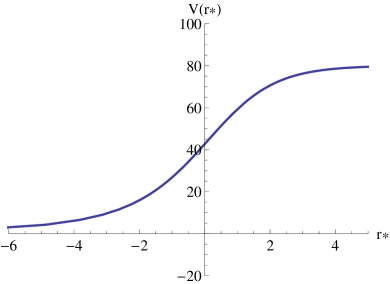
Figure 1: The behavior of the potential $V(r)$ plotted against $r_{*}$. Here, $M=10,m=2$ and $\Lambda=2$.

4 Exact solutions to the scalar wave equation

In order to find exact solutions to the wave equation for the massless scalar, we will revisit the Eq. $(\ref{klein})$ in section 3 with the anzatz,

$$\Phi=e^{-i\omega t}e^{im\theta}R(r)$$ (13)

Eq. $(\ref{klein})$ leads to the radial equation,

$$\frac{d}{dr}\left(\frac{f(r)}{2}\frac{dR(r)}{dr}\right)+2r^{2}\left(\frac{\omega^{2}}{f(r)}-\frac{m^{2}}{r^{2}}\right)R(r)=0\,.$$ (14)

In order to solve the wave equation exactly, we will redefine $r$ coordinate of the Eq. $(\ref{metric})$ with a new variable $x$ given by,

$$x=\left(\frac{r_{h}}{r-r_{h}}\right)\,.$$ (15)

In the new coordinate system, $x=0$ corresponds to $r\rightarrow\infty$ and $x=\infty$ corresponds $r=r_{h}$. With the new coordinate, Eq. $(\ref{wave})$ becomes,

$$\frac{d^{2}R}{dx^{2}}+\left(\frac{A}{x^{2}}+\frac{B}{x}+C\right)R=0$$ (16)

where,

$$A=\frac{\omega^{2}}{16\Lambda^{2}}-\frac{m^{2}}{2\Lambda}\,,$$

$$B=\frac{\omega^{2}}{8\Lambda^{2}}\,,$$

$$C=\frac{\omega^{2}}{16\Lambda^{2}}\,.$$ (17)

The Eq. $(\ref{wave2})$ resembles the Whittaker differential equation given by [53],

$$\frac{d^{2}R}{dz^{2}}+\left(\frac{\frac{1}{4}-\mu^{2}}{z^{2}}+\frac{\kappa}{z}-\frac{1}{4}\right)R=0\,.$$ (18)

The solutions to the Whittaker equation are given by,

$$M_{\kappa,\mu}(z)=e^{-\frac{z}{2}}z^{\frac{1}{2}+\mu}M[\frac{1}{2}+\mu-\kappa,1+2\mu,z]\,,$$

and

$$M_{\kappa,-\mu}(z)=e^{-\frac{z}{2}}z^{\frac{1}{2}-\mu}M[\frac{1}{2}-\mu-\kappa,1-2\mu,z]\,.$$ (19)

The function $M[a,b,z]$ is called the $KummerFunction$ and is the solution to the Kummer differential equation given by [53],

$$z\frac{d^{2}F}{dz^{2}}+(b-z)\frac{dF}{dz}-aF=0\,.$$ (20)

Now, to transform the Eq. $(\ref{wave2})$ to the Whittaker form, we will reparametrize the coordinate $x$ as

$$y=i2\sqrt{C}x=\frac{i\omega}{2\Lambda}x\,.$$ (21)

Then the Eq. $(\ref{wave2})$ takes the form,

$$\frac{d^{2}R}{dy^{2}}+\left(\frac{\frac{1}{4}-\mu^{2}}{y^{2}}+\frac{\kappa}{y}-\frac{1}{4}\right)R=0\,,$$ (22)

with

$$\kappa=\frac{i\omega}{4\Lambda};\hskip 14.22636pt\mu=\frac{i}{2}\sqrt{\frac{\omega^{2}-8m^{2}\Lambda}{4\Lambda^{2}}-1}\,.$$ (23)

Note that we will take $``+^{\prime\prime}$ sign without loss of generality. Before presenting the final form of the solution to the wave equation, we will redefine the parameters $\kappa$ and $\mu$ with $\alpha$ and $\beta$ as,

$$\kappa=\alpha;\hskip 56.9055pt\mu=\beta-\frac{1}{2}\,.$$ (24)

The reason to introduce the new parameters is to follow the same notation followed with the computation done for the non-extreme black hole by the same author in [54]. Finally, by substituting the values of $\kappa$ and $\mu$ in terms of $\alpha$ and $\beta$, the general solution to the wave equation can be written as

$$R(y)=C_{1}e^{-\frac{y}{2}}y^{\beta}F[\beta-\alpha,2\beta,y]+C_{2}e^{-\frac{y}{2}}y^{1-\beta}F[1-\beta-\alpha,2(1-\beta),y]\,.$$ (25)

Hence the general solution to the waves equation is,

$$\Phi(y,t,\theta)=e^{im\theta}e^{-i\omega t}R(y)\,.$$ (26)

5 Quasinormal modes of the extreme dilaton black holes

Since the main objective of the paper is to find QNMs of the extreme black hole, one needs to impose specific boundary conditions to the general solution obtained in section 4. The solutions are analyzed closer to the horizon and at infinity to obtain exact results for QNMs.

To compute QNMs of a black hole, two boundary conditions are imposed. One is to impose the wave to be purely ingoing at he horizon. The other is the boundary condition for large $r$ values. For asymptotically flat space-times, the asymptotic boundary condition is for the field to be purely out going. For non-asymptotically-flat space-times, there are two possibilities: on is for the field to vanish and the other is for the flux to vanish. We choose the field to vanish similar to what was done in [54].

5.1 Solution at asymptotic region

First we will study what the solution is when $r\rightarrow\infty$. Since for large $r$, $y\rightarrow 0$, the Kummer function $M[a,b,y]\rightarrow 1$. By substituting $y\rightarrow 0$ to the exact solution obtained for $R(y)$, one obtain,

$$R(r\rightarrow\infty,r\rightarrow 0)\approx C_{1}y^{\beta}+C_{2}y^{1-\beta}\,.$$ (27)

Since,

$$y=\frac{i\omega r_{h}}{2\Lambda(r-r_{h})}$$ (28)

for large $r$,

$$y\rightarrow\frac{i\hat{\omega}}{2\Lambda}\left(\frac{r_{h}}{r}\right)$$ (29)

the Eq. (27) can be written in terms of $r$ as,

$$R(r\rightarrow\infty)\approx C_{1}\left(\frac{i\hat{\omega}}{2\Lambda}\right)^{\beta}\left(\frac{r_{h}}{r}\right)^{\beta}+C_{2}\left(\frac{i\hat{\omega}}{2\Lambda}\right)^{1-\beta}\left(\frac{r_{h}}{r}\right)^{1-\beta}\,.$$ (30)

Now one need to determine which part of the solution in Eq. (30) corresponds to the “ingoing” and “outgoing” respectively. For that we will first find the tortoise coordinate $r_{*}$ in terms of $r$ at large $r$. Note that for large $r$, $f(r)\rightarrow 8\Lambda r^{2}$. Hence the equation relating the tortoise coordinate $r_{*}$ and $r$ in Eq. $(\ref{tor})$ simplifies to,

$$dr_{*}=\frac{dr}{4\Lambda r}\,.$$ (31)

The above can be integrated to obtain,

$$r_{*}\approx\frac{1}{4\Lambda}ln(\frac{r}{r_{h}})\,.$$ (32)

Hence,

$$r\approx r_{h}e^{4\Lambda r_{*}}\,.$$ (33)

Substituting $r$ from Eq. (33) and $\beta$ from Eq. (24) into the Eq. (30), $R(r\rightarrow\infty)$ is rewritten as,

$$R(r\rightarrow\infty)\rightarrow C_{1}\left(\frac{i\hat{\omega}}{2\Lambda}\right)^{\beta}e^{-i\omega r_{*}\sqrt{1-\frac{4\Lambda^{2}}{\omega^{2}}(\frac{2m^{2}}{\Lambda}+1)}-2\Lambda r_{*}}$$

$$+C_{2}\left(\frac{i\hat{\omega}}{2\Lambda}\right)^{1-\beta}e^{i\omega r_{*}\sqrt{1-\frac{4\Lambda^{2}}{\omega^{2}}(\frac{2m^{2}}{\Lambda}+1)}-2\Lambda r_{*}}\,.$$ (34)

From the above one can conclude that the first term and the second term represents the ingoing and outgoing waves respectively. Since for QNMs, the ingoing amplitude has to be zero, we chose $C_{1}=0$. Hence the solution to the wave equation becomes,

$$R(y)=C_{2}e^{-\frac{y}{2}}y^{1-\beta}M[1-\beta-\alpha,2(1-\beta),y]\,.$$ (35)

5.2 Solutions near the horizon

Now we can analyze the solution of the wave equation near the horizon ($r\rightarrow r_{h}$, $y\rightarrow\infty$). The Kummer function $M[a,c,y]$ has an expansion for large $y$ as follows [53],

$$F[a,c,y]\rightarrow e^{y}y^{a-c}\frac{\Gamma(c)}{\Gamma(a)}+e^{\pm i\pi a}y^{-a}\frac{\Gamma(c)}{\Gamma(c-a)}\,.$$ (36)

Note that the upper sign is taken if $-\frac{\pi}{2}<arg(y)<\frac{3\pi}{2}$ and lower sign is chosen $-\frac{3\pi}{2}<arg(y)<-\frac{\pi}{2}$. Since $arg(y)=\frac{\pi}{2}$ the upper sign will be chosen. By substituting the above expansion with the appropriate values for $a$ and $c$ in terms of $\alpha$ and $\beta$, one obtain the function $R(y)$ near the horizon as,

$$R(r\rightarrow r_{h},y\rightarrow\infty)\rightarrow C_{2}\left(e^{y/2}y^{-\alpha}\frac{\Gamma(2-2\beta)}{\Gamma(1-\beta-\alpha)}+e^{-y/2+i\pi(1-\beta-\alpha)}y^{\alpha}\frac{\Gamma(2-2\beta)}{\Gamma(1-\beta+\alpha)}\right)\,.$$ (37)

To determine which part of the above equation represents the ingoing/outgoing, one has to introduce the tortoise coordinate near the horizon. From Eq. $(\ref{tor})$, the tortoise coordinate near the horizon can be approximated with,

$$r_{*}\approx\frac{1}{4\Lambda}ln(r-r_{h})\rightarrow e^{-4\Lambda r_{*}}\approx\frac{1}{(r-r_{h})}\,.$$ (38)

By substituting $y$ in terms of $r_{*}$ in Eq. $(\ref{newtor2})$, the radial function $R(r_{*})$ approximates to,

$$R(r\rightarrow r_{h},y\rightarrow\infty)\approx C_{2}e^{\frac{y}{2}}\frac{\Gamma(2-2\beta)}{\Gamma(1-\beta-\alpha)}\left(\frac{i\hat{\omega}r_{h}}{2\Lambda}\right)^{-\alpha}e^{i\omega r_{*}}+$$

$$C_{2}e^{-\frac{y}{2}+i\pi(1-\beta-\alpha)}\frac{\Gamma(2-2\beta)}{\Gamma(1-\beta+\alpha)}\left(\frac{i\hat{\omega}r_{h}}{2\Lambda}\right)^{\alpha}e^{-i\omega r_{*}}\,.$$ (39)

The first represents the outgoing waves and the second represents the ingoing wave at the horizon.

5.3 Quasinormal modes

Since the QNMs are defined with as purely ingoing waves at the horizon, the outgoing terms has to be zero. Since $C_{2}\neq 0$, the first term vanish only at the poles of the Gamma function, $\Gamma(1-\beta-\alpha)$. Note that the Gamma function $\Gamma(x)$ has poles at $x=-n$ for $n=0,1,2..$. Hence to obtain QNMs, the following relations has to hold.

$$1-\alpha-\beta=-n$$ (40)

leading to,

$$\beta=(1+n)-\frac{i\omega}{4\Lambda}\,.$$ (41)

By combining Eq. $(\ref{qnm1})$ and Eq. $(\ref{qnm2})$, one can solve for $\omega$ as,

$$\omega=\frac{-2i}{2n+1}\left(2\Lambda n(1+n)-m^{2}\right)\,.$$ (42)

They are pure imaginary, do not depend on the black hole parameters, and the decay rate increases when the cosmological constant increases. Note that the fundamental mode $n=0$ is unstable, and the decay rate depends only on the angular number of the test field. Due to the minus sign in front, these oscillations will be damped leading to stable perturbations for $2\Lambda n(1+n)>m^{2}$. However, for $2\Lambda n(1+n)<m^{2}$, the oscillations would lead to unstable modes.

In acoustic black holes, QNM’s for scalar field shows similar properties [55]. There,

$$\omega=-\frac{i}{2}\frac{(n-1)(n+3)\tilde{a}}{n+1}\,.$$ (43)

For $n=0$, $\omega$ is positive and will lead to exponentially growing mode similar to the extreme dilaton black hole discussed above.

6 Numerical analysis

Some well known numerical methods to obtain QNM frequencies are: the Mashhoon method, Chandrasekhar-Detweiler method, WKB method, Frobenius method, continued fraction method, asymptotic iteration method (AIM) and improved AIM, pseudospectral Chebyshev method, among others. In this section, we apply the improved AIM [56] method to compare with the analytical results. This is an improved version of the method proposed in Refs. [57, 58] and it has been applied successfully in the context of QNMs for different black holes geometries; see for instance [59, 60, 61, 62, 63, 68, 64, 65, 66, 67].

The boundary conditions satisfied by the QNMs are given by

$$\xi\sim e^{-i\omega r_{\ast}}\,\,\, \text{as}\,\,\,r_{\ast}\rightarrow-\infty$$

$$\xi\sim e^{i\tilde{\omega}r_{\ast}}\,\,\, \text{as}\,\,\,r_{\ast}\rightarrow\infty$$

where $\tilde{\omega}^{2}=\omega^{2}-4\Lambda^{2}-8\Lambda m^{2}$. There are only ingoing waves at the horizon and outgoing waves at infinity. This can be transformed to

$$R\sim r^{-\frac{1}{2}}(r-r_{h})^{-\frac{i\omega}{4\Lambda}}e^{\frac{i\omega}{4\Lambda}\frac{r_{h}}{r-r_{h}}}\,\,\, \text{as}\,\,\,r\rightarrow r_{h}$$

$$R\sim r^{-\frac{1}{2}+\frac{i\tilde{\omega}}{4\Lambda}}\,\,\, \text{as}\,\,\,r\rightarrow\infty$$

In order to write a solution with this behavior at the boundaries, we define

$$R(r)=r^{-\frac{1}{2}+\frac{i(\tilde{\omega}+\omega)}{4\Lambda}}(r-r_{h})^{-\frac{i\omega}{4\Lambda}}e^{\frac{i\omega r_{h}}{4\Lambda(r-r_{h})}}\chi(r)\,.$$ (44)

Inserting this expression in Eq. (14) and performing the change of variable $z=1-r_{h}/r$ we arrive at the following equation

$$\chi^{\prime\prime}(z)=\lambda_{0}(z)\chi^{\prime}(z)+s_{0}(z)\chi\,,$$ (45)

where the prime denotes derivative with respect to $z$ and

$$\lambda_{0}(z) = -\frac{1}{2(1-z)z^{2}\Lambda}\left(-i\omega+4\Lambda z+z^{2}\left(i\omega-6\Lambda+\sqrt{-\omega^{2}+4\Lambda^{2}+8\Lambda m^{2}}\right)\right)$$

$$s_{0}(z) = -\frac{1}{8(1-z)z^{2}\Lambda^{2}}\Big{(}\omega^{2}-i\omega\sqrt{-\omega^{2}+4\Lambda^{2}+8\Lambda m^{2}}-4\Lambda m^{2}+z(\omega^{2}+4i\omega\Lambda-$$ (46)

$$4\Lambda m^{2}-8\Lambda^{2}+4\Lambda\sqrt{-\omega^{2}+4\Lambda^{2}+8\Lambda m^{2}}-i\omega\sqrt{-\omega^{2}+4\Lambda^{2}+8\Lambda m^{2}})\Big{)}\,.$$

We solve numerically Eq. (45) using the improved AIM. This method is implemented as follows, first it is necessary to differentiate Eq. (45) $n$ times with respect to $z$, what yields

$$\chi^{n+2}=\lambda_{n}(z)\chi^{\prime}+s_{n}(z)\chi\,,$$ (47)

where

$$\lambda_{n}(z) = \lambda^{\prime}_{n-1}(z)+s_{n-1}(z)+\lambda_{0}(z)\lambda_{n-1}(z)$$

$$s_{n}(z) = s^{\prime}_{n-1}(z)+s_{0}(z)\lambda_{n-1}(z)\,.$$ (48)

Then, the functions $\lambda_{n}$ and $s_{n}$ are Taylor expanded around some point $z_{0}$ ($0<z_{0}<1$) at which the improved AIM is performed

$$\lambda_{n}(z_{0}) = \sum_{i=0}^{\infty}c_{n}^{i}(z-z_{0})^{i}$$

$$s_{n}(z_{0}) = \sum_{i=0}^{\infty}d_{n}^{i}(z-z_{0})^{i}\,,$$

$c_{n}^{i}$ and $d_{n}^{i}$ are the i^th Taylor coefficients of $\lambda_{n}(z_{0})$ and $s_{n}(z_{0})$ respectively. Then, replacing these Taylor expansions in Eqs. (6) the following set of recursion relations for the coefficients are obtained

$$c_{n}^{i} = (i+1)c_{n-1}^{i+1}+d_{n-1}^{i}+\sum_{k=0}^{i}c_{0}^{k}c_{n-1}^{i-k}$$

$$d_{n}^{i} = (i+1)d_{n-1}^{i+1}+\sum_{k=0}^{i}d_{0}^{k}c_{n-1}^{i-k}\,.$$

Next, imposing a termination to the number of iterations one arrives to the following quantization condition

$$d_{n}^{0}c_{n-1}^{0}-d_{n-1}^{0}c_{n}^{0}=0\,.$$ (49)

We use a root-finding algorithm to determine numerically the QNFs from (49). In Table 1 we show some values of QNFs, in order to check the correctness and accuracy of the numerical technique used. The numerical values where round to five decimal places and they show a good and exact agreement with the exact result via Eq. (42). As it was mentioned, these oscillations will be damped leading to stable perturbations for $2\Lambda n(1+n)>m^{2}$. However, for $2\Lambda n(1+n)<m^{2}$, the oscillations would lead to unstable modes.

Table 1: QNFs for massless scalar fields with $\Lambda=1,m=3$ in the background of tree-dimensional extreme dilaton black holes.

$n$	$\omega_{AIM}$	$\omega$
$0$	$18.00000i$	$18i$
$1$	$3.33333i$	$10/3i$
$2$	$-1.20000i$	$-6/5i$
$3$	$-4.28571i$	$-30/7i$
$4$	$-6.88889i$	$-62/9i$

7 Conclusion

In this work we considered the propagation of massless scalar fields in the background of three-dimensional extremal dilaton black holes. We obtained QNM frequencies analytically, and we showed that the QNMs are overdamped or purely imaginary leading to stable perturbations for $2\Lambda n(1+n)>m^{2}$. For $2\Lambda n(1+n)<m^{2}$ the oscillations would lead to unstable modes. The decay rate increases when the cosmological constant increases. For the fundamental mode $n=0$, the decay rate depends only on the angular number of the test field: however in this case the modes are unstable. Also, we used the improved AIM in order to determine the QNFs numericaly, and we showed that there is a good agreement between the numerical and the analytical solutions.

There are number of works that are interesting to do in the future related to this work presented here: Onozawa et.al [69] showed that QNM’s for the extreme Reissner-Nordström black holes for the spin 1, 3/2, 2 are the same. It would be interesting to see if that is the case for the extreme dilaton black hole. It would also be interesting to analyze the superradiant instability [70] of this extremal black hole for charged massive scalar field, as well as, the quasinormal modes: we leave those for a future work, see [71].

References

- [1] S. W. Hawking, G.T. Horowitz, and S. F. Ross, “Entropy, area, and black hole pairs,” Phys. Rev. D 51, 4302 (1995) [arXiv: 9409013 [gr-qc]]
- [2] R. Kallosh, A. Linde, T. Orten, and A. Peet, “Supersymmetry as a cosmic censor,” Phys. Re. D 46 (1992) 5278 [arXiv: 9205027[hep-th]]
- [3] Sen, “Microscopic and macroscopic entropy of extremal black holes in string theory,” [arXiv:1402.0109[hep-t]]
- [4] I. Mandal and A. Sen, “Black hole microstate counting and macro state counterpart,” Nucl. Phys. Proc. Suppl. 216, 147 (2011) [arXiv:1008.3801[hep-th]]
- [5] R. A. Konoplya and A. Zhidenko, “Quasinormal modes of black holes: From astrophysics to string theory,” Rev. Mod. Phys. 83, 793 (2011), [arXiv:1102.4014 [gr-qc]].
- [6] T. Regge and J.A. Wheeler, Stability of a Schwarzschild singularity, Phys. Rev. 108 (1957) 1063.
- [7] F. J. Zerilli, “Gravitational field of a particle falling in a schwarzschild geometry analyzed in tensor harmonics,” Phys. Rev. D 2, 2141 (1970).
- [8] F. J. Zerilli, “Effective potential for even parity Regge-Wheeler gravitational perturbation equations,” Phys. Rev. Lett. 24, 737 (1970).
- [9] K. D. Kokkotas and B. G. Schmidt, “Quasinormal modes of stars and black holes,” Living Rev. Rel. 2, 2 (1999) [gr-qc/9909058].
- [10] H. -P. Nollert, “TOPICAL REVIEW: Quasinormal modes: the characteristic ‘sound’ of black holes and neutron stars,” Class. Quant. Grav. 16, R159 (1999).
- [11] B. P. Abbott et al. [LIGO Scientific and Virgo Collaborations], “Observation of Gravitational Waves from a Binary Black Hole Merger,” Phys. Rev. Lett. 116, no. 6, 061102 (2016)
- [12] B. P. Abbott et al. [LIGO Scientific and Virgo Collaborations], “Tests of general relativity with GW150914,” Phys. Rev. Lett. 116, no. 22, 221101 (2016)
- [13] J. Crisóstomo, S. Lepe and J. Saavedra, “Quasinormal modes of extremal BTZ black hole,” Class. Quant. Grav. 21, 2801-2810 (2004) [arXiv:hep-th/0402048 [hep-th]].
- [14] H. Onozawa, T. Mishima, T. Okamura and H. Ishihara, “Quasinormal modes of maximally charged black holes,” Phys. Rev. D 53 (1996), 7033-7040 [arXiv:gr-qc/9603021 [gr-qc]].
- [15] M. Richartz, “Quasinormal modes of extremal black holes,” Phys. Rev. D 93 (2016) no.6, 064062 [arXiv:1509.04260 [gr-qc]].
- [16] E. Berti and K. D. Kokkotas, “Quasinormal modes of Reissner-Nordström-anti-de Sitter black holes: Scalar, electromagnetic and gravitational perturbations,” Phys. Rev. D 67 (2003), 064020 [arXiv:gr-qc/0301052 [gr-qc]].
- [17] M. Richartz and D. Giugno, “Quasinormal modes of charged fields around a Reissner-Nordström black hole,” Phys. Rev. D 90 (2014) no.12, 124011 [arXiv:1409.7440 [gr-qc]].
- [18] V. Cardoso, J. L. Costa, K. Destounis, P. Hintz and A. Jansen, “Quasinormal modes and Strong Cosmic Censorship,” Phys. Rev. Lett. 120 (2018) no.3, 031103 [arXiv:1711.10502 [gr-qc]].
- [19] V. Cardoso, J. L. Costa, K. Destounis, P. Hintz and A. Jansen, “Strong cosmic censorship in charged black-hole spacetimes: still subtle,” Phys. Rev. D 98 (2018) no.10, 104007 [arXiv:1808.03631 [gr-qc]].
- [20] K. Destounis, “Charged Fermions and Strong Cosmic Censorship,” Phys. Lett. B 795 (2019), 211-219 [arXiv:1811.10629 [gr-qc]].
- [21] G. Panotopoulos, “Charged scalar fields around Einstein-power-Maxwell black holes,” Gen. Rel. Grav. 51 (2019) no.6, 76
- [22] H. Liu, Z. Tang, K. Destounis, B. Wang, E. Papantonopoulos and H. Zhang, “Strong Cosmic Censorship in higher-dimensional Reissner-Nordström-de Sitter spacetime,” JHEP 03 (2019), 187 [arXiv:1902.01865 [gr-qc]].
- [23] K. Destounis, “Superradiant instability of charged scalar fields in higher-dimensional Reissner-Nordström-de Sitter black holes,” Phys. Rev. D 100 (2019) no.4, 044054 [arXiv:1908.06117 [gr-qc]].
- [24] K. Destounis, R. D. B. Fontana, F. C. Mena and E. Papantonopoulos, “Strong Cosmic Censorship in Horndeski Theory,” JHEP 10 (2019), 280 [arXiv:1908.09842 [gr-qc]].
- [25] K. Destounis, R. D. B. Fontana and F. C. Mena, “Accelerating black holes: quasinormal modes and late-time tails,” Phys. Rev. D 102 (2020) no.4, 044005 [arXiv:2005.03028 [gr-qc]].
- [26] K. Destounis, R. D. B. Fontana and F. C. Mena, “Stability of the Cauchy horizon in accelerating black-hole spacetimes,” Phys. Rev. D 102 (2020) no.10, 104037 [arXiv:2006.01152 [gr-qc]].
- [27] A. Aragón, P. A. González, J. Saavedra and Y. Vásquez, “Scalar quasinormal modes for -dimensional Coulomb-like AdS black holes from nonlinear electrodynamics,” Gen. Rel. Grav. 53 (2021) no.10, 91 [arXiv:2104.08603 [gr-qc]].
- [28] R. D. B. Fontana, P. A. González, E. Papantonopoulos and Y. Vásquez, “Anomalous decay rate of quasinormal modes in Reissner-Nordström black holes,” Phys. Rev. D 103 (2021) no.6, 064005 [arXiv:2011.10620 [gr-qc]].
- [29] E. Witten, “On black holes in string theory,” [arXiv:hep-th/9111052 [hep-th]].
- [30] E. Teo, “Statistical entropy of charged two-dimensional black holes,” Phys. Lett. B 430 (1998), 57-62 [arXiv:hep-th/9803064 [hep-th]].
- [31] M. D. McGuigan, C. R. Nappi and S. A. Yost, “Charged black holes in two-dimensional string theory,” Nucl. Phys. B 375 (1992), 421-450 [arXiv:hep-th/9111038 [hep-th]].
- [32] V. Ferrari, M. Pauri and F. Piazza, “Quasinormal modes of charged, dilaton black holes,” Phys. Rev. D 63 (2001), 064009 [arXiv:gr-qc/0005125 [gr-qc]].
- [33] R. A. Konoplya, “Quasinormal modes of the electrically charged dilaton black hole,” Gen. Rel. Grav. 34 (2002), 329-335 [arXiv:gr-qc/0109096 [gr-qc]].
- [34] S. Fernando, “Quasinormal modes of charged dilaton black holes in (2+1)-dimensions,” Gen. Rel. Grav. 36 (2004), 71-82 [arXiv:hep-th/0306214 [hep-th]].
- [35] J. Kettner, G. Kunstatter and A. J. M. Medved, “Quasinormal modes for single horizon black holes in generic 2-d dilaton gravity,” Class. Quant. Grav. 21 (2004), 5317-5332 [arXiv:gr-qc/0408042 [gr-qc]].
- [36] S. b. Chen and J. l. Jing, “Asymptotic quasinormal modes of a coupled scalar field in the Garfinkle-Horowitz-Strominger dilaton spacetime,” Class. Quant. Grav. 22 (2005), 533-540 [arXiv:gr-qc/0409013 [gr-qc]].
- [37] S. B. Chen and J. L. Jing, “Dirac quasinormal modes of the Garfinkle-Horowitz-Strominger dilaton black-hole spacetime,” Class. Quant. Grav. 22 (2005), 1129-1141
- [38] S. B. Chen and J. L. Jing, “Asymptotic quasinormal modes of a coupled scalar field in the Gibbons-Maeda dilaton spacetime,” Class. Quant. Grav. 22 (2005), 2159-2165 [arXiv:gr-qc/0511106 [gr-qc]].
- [39] S. Fernando, “Quasinormal modes of charged scalars around dilaton black holes in 2+1 dimensions: Exact frequencies,” Phys. Rev. D 77 (2008), 124005 [arXiv:0802.3321 [hep-th]].
- [40] Y. S. Myung, Y. W. Kim and Y. J. Park, “Quasinormal modes from potentials surrounding the charged dilaton black hole,” Eur. Phys. J. C 58 (2008), 617-625 [arXiv:0809.1933 [gr-qc]].
- [41] K. Lin, “Gravitational perturbation of Garfinkle-Horowitz-Strominger dilaton black hole and quasinormal modes,” Int. J. Theor. Phys. 49 (2010), 2786-2792
- [42] I. Sakalli, “Quasinormal modes of charged dilaton black holes and their entropy spectra,” Mod. Phys. Lett. A 28 (2013), 1350109 [arXiv:1307.0340 [gr-qc]].
- [43] R. Becar, P. A. Gonzalez and Y. Vasquez, “Dirac quasinormal modes of two-dimensional charged Dilatonic Black Holes,” Eur. Phys. J. C 74 (2014), 2940 [arXiv:1405.1509 [gr-qc]].
- [44] S. Fernando, “Quasinormal modes of dilaton-de Sitter black holes: scalar perturbations,” Gen. Rel. Grav. 48 (2016) no.3, 24 [arXiv:1601.06407 [gr-qc]].
- [45] J. L. Blázquez-Salcedo, F. S. Khoo and J. Kunz, “Quasinormal modes of Einstein-Gauss-Bonnet-dilaton black holes,” Phys. Rev. D 96 (2017) no.6, 064008 [arXiv:1706.03262 [gr-qc]].
- [46] K. Destounis, G. Panotopoulos and Á. Rincón, “Stability under scalar perturbations and quasinormal modes of 4D Einstein–Born–Infeld dilaton spacetime: exact spectrum,” Eur. Phys. J. C 78 (2018) no.2, 139 [arXiv:1801.08955 [gr-qc]].
- [47] R. Brito and C. Pacilio, “Quasinormal modes of weakly charged Einstein-Maxwell-dilaton black holes,” Phys. Rev. D 98 (2018) no.10, 104042 [arXiv:1807.09081 [gr-qc]].
- [48] A. F. Zinhailo, “Quasinormal modes of Dirac field in the Einstein–Dilaton–Gauss–Bonnet and Einstein–Weyl gravities,” Eur. Phys. J. C 79 (2019) no.11, 912 [arXiv:1909.12664 [gr-qc]].
- [49] A. Rincon and G. Panotopoulos, “Quasinormal modes of black holes with a scalar hair in Einstein-Maxwell-dilaton theory,” Phys. Scripta 95 (2020) no.8, 085303 [arXiv:2007.01717 [gr-qc]].
- [50] K. C. K. Chan, R. B. Mann, Static charged black holes in 2+1 dimensional dilaton gravity , Phys. Rev. D50 6385 ( 1994)
- [51] Y. S. Myung, Y. Kim & Y. Park, Quasinormal modes from potentials surrounding the charged dilaton black hole, Eur. Phys. Jour. C58 617 (2008)
- [52] A. Lopez-Ortega, Quasinormal modes and stability of a five-dimensional dilatonic black hole, Int. Jour. Mod. Phys. D18 1441 (2009)
- [53] M. Abramowitz & A. Stegun, Handbook of Mathematical Functions Dover, (1977)
- [54] S. Fernando, Quasinormal modes of charged dilaton black holes in 2+1 dimensions , Gen. Rel. Grav. 36 71 (2004)
- [55] J. Saavedra, ”Quasinormal modes of Unruh’s acoustic black holes,” Mod.Phys.Lett. A21 (2006) 1601
- [56] H. T. Cho, A. S. Cornell, J. Doukas and W. Naylor, “Black hole quasinormal modes using the asymptotic iteration method,” Class. Quant. Grav. 27 (2010), 155004 [arXiv:0912.2740 [gr-qc]].
- [57] H. Ciftci, R. L. Hall, and N. Saad, “Asymptotic iteration method for eigenvalue problems,” J. Phys. A 36(47), 11807-11816 (2003).
- [58] H. Ciftci, R. L. Hall and N. Saad, “Perturbation theory in a framework of iteration methods,” Phys. Lett. A 340 (2005), 388-396 [arXiv:math-ph/0504056 [math-ph]].
- [59] H. T. Cho, A. S. Cornell, J. Doukas, T. R. Huang and W. Naylor, “A New Approach to Black Hole Quasinormal Modes: A Review of the Asymptotic Iteration Method,” Adv. Math. Phys. 2012 (2012), 281705 [arXiv:1111.5024 [gr-qc]].
- [60] M. Catalan, E. Cisternas, P. A. Gonzalez and Y. Vasquez, “Dirac quasinormal modes for a 4-dimensional Lifshitz black hole,” Eur. Phys. J. C 74 (2014) no.3, 2813 [arXiv:1312.6451 [gr-qc]].
- [61] C. Y. Zhang, S. J. Zhang and B. Wang, Nucl. Phys. B 899 (2015), 37-54 doi:10.1016/j.nuclphysb.2015.07.030 [arXiv:1501.03260 [hep-th]].
- [62] T. Barakat, “The asymptotic iteration method for Dirac and Klein-Gordon equations with a linear scalar potential,” Int. J. Mod. Phys. A 21 (2006), 4127-4135
- [63] W. Sybesma and S. Vandoren, “Lifshitz quasinormal modes and relaxation from holography,” JHEP 05 (2015), 021 [arXiv:1503.07457 [hep-th]].
- [64] M. Catalán, E. Cisternas, P. A. González and Y. Vásquez, “Quasinormal modes and greybody factors of a four-dimensional Lifshitz black hole with z=0,” Astrophys. Space Sci. 361 (2016) no.6, 189 [arXiv:1404.3172 [gr-qc]].
- [65] P. A. González and Y. Vásquez, “Scalar Perturbations of Nonlinear Charged Lifshitz Black Branes with Hyperscaling Violation,” Astrophys. Space Sci. 361 (2016) no.7, 224 [arXiv:1509.00802 [hep-th]].
- [66] R. Becar, P. A. Gonzalez and Y. Vasquez, “Quasinormal modes of Four Dimensional Topological Nonlinear Charged Lifshitz Black Holes,” Eur. Phys. J. C 76 (2016) no.2, 78 [arXiv:1510.06012 [gr-qc]].
- [67] R. Bécar, P. A. González and Y. Vásquez, “Quasinormal modes of non-Abelian hyperscaling violating Lifshitz black holes,” Gen. Rel. Grav. 49 (2017) no.2, 26 [arXiv:1510.04605 [hep-th]].
- [68] C. H. Chen, H. T. Cho, A. S. Cornell, G. Harmsen and W. Naylor, “Gravitino fields in Schwarzschild black hole spacetimes,” Chin. J. Phys. 53 (2015), 110101 doi:10.6122/CJP.20150511 [arXiv:1504.02579 [gr-qc]].
- [69] H. Onozawa, T. Okamura, T. Mishima, and H. Ishihara, ”Perturbing supersymmetric black holes,” Phys.Rev.D 55(1997), 4529 [arXiv:9606086 [gr-qc]]
- [70] R. Brito, V. Cardoso and P. Pani, “Superradiance: New Frontiers in Black Hole Physics,” Lect. Notes Phys. 906 (2015), pp.1-237 [arXiv:1501.06570 [gr-qc]].
- [71] P. A. González, Á. Rincón, J. Saavedra and Y. Vásquez, “Superradiant instability and charged scalar quasinormal modes for (2+1)-dimensional Coulomb-like AdS black holes from nonlinear electrodynamics,” Phys. Rev. D 104 (2021) no.8, 084047 [arXiv:2107.08611 [gr-qc]].