Revealing directed effective connectivity of cortical neuronal networks from measurements

Abstract

In the study of biological networks, one of the major challenges is to understand the relationships between network structure and dynamics. In this paper, we model in vitro cortical neuronal cultures as stochastic dynamical systems and apply a method that reconstructs directed networks from dynamics [Ching and Tam, Phys. Rev. E 95, 010301(R), 2017] to reveal directed effective connectivity, namely the directed links and synaptic weights, of the neuronal cultures from voltage measurements recorded by a multielectrode array. The effective connectivity so obtained reproduces several features of cortical regions in rats and monkeys and has similar network properties as the synaptic network of the nematode C. elegans, the only organism whose entire nervous system has been mapped out as of today. The distribution of the incoming degree is bimodal and the distributions of the average incoming and outgoing synaptic strength are non-Gaussian with long tails. The effective connectivity captures different information from the commonly studied functional connectivity, estimated using statistical correlation between spiking activities. The average synaptic strengths of excitatory incoming and outgoing links are found to increase with the spiking activity in the estimated effective connectivity but not in the functional connectivity estimated using the same sets of voltage measurements. These results thus demonstrate that the reconstructed effective connectivity can capture the general properties of synaptic connections and better reveal relationships between network structure and dynamics.

I Introduction

The study of networks Strogatz ; AlbertBarabasi ; Newman has emerged in many branches of science. Many systems of interest consist of a large number of components that interact with each other and can be described as complex networks with the individual components being the nodes and the interactions among the nodes represented by links joining the nodes. Understanding how network structure, which depicts the connectivity or linkage of nodes, is related to dynamics and to function is a great challenge in neuroscience Bullmore2009 ; Bassett2017 and in biology in general. In neuroscience, three types of connectivity have been discussed: structural, functional and effective connectivity. Structural connectivity is the set of physical or anatomical connections linking neural elements and can be obtained only by direct measurements, functional connectivity is defined by statistical dependencies among measurements of neuronal activities, and effective connectivity refers to the causal influences exerted by one neural element on another (see e.g. Friston2011 ; Sporns2011 ). As statistical dependency can arise from indirect interactions, functional connectivity does not necessarily relate to effective connectivity. Effective connectivity depends on structure connectivity in that a neural element can exert causal influences on another neural element only if the former is linked to the latter by anatomical connections but structural connectivity itself does not imply effective connectivity since it is possible that some physical connections are not being utilized in certain neuronal activities.

Neuronal cultures grown in vitro serve as a simple but yet useful experimental model system for studying the relationships between network structure and the rich dynamics observed Eckmann2007 ; Feinerman2008 ; Soriano2015 . One common technique used to record the activity of neurons in a culture is the measurement of the voltage signals generated by neurons using a multielectrode array (MEA) Obien2015 . Estimating connectivity of neuronal cultures from MEA recordings is thus a problem of great interest. Existing methods focus on estimating functional connectivity of neuronal culture using statistical correlation Maccione2012 ; Poli2015 ; Pastore2018 or mutual information Bettencourt2007 ; Bettencourt2008 of detected spikes in the MEA recordings. However, one would expect effective connectivity that gives direct causal influences or interactions to be more relevant for studying the relationships between network structure and dynamics and between network structure and function.

The general problem of inferring networks from dynamics for networked systems whose interacting dynamics are described by systems of coupled differential equations is a problem of longstanding interest TimmeReview . It has been known that statistical correlation often fails to be a good indicator for direct interactions. There are analytical results showing that the statistical covariance of nodal dynamics alone does not carry sufficient information to recover networks with directional coupling Gilson2016 ; PhysicaA2018 . For a certain class of undirected networked systems with bidirectional coupling, it has been derived that effective connectivity or the information of direct interactions is contained in the inverse of the covariance matrix and not the covariance matrix itself noisePRL ; PRE ; PRErapid . This result can therefore explain the finding that a neural population can be strongly coupled but have weak pairwise correlation weak . A number of methods inferring direct interactions from dynamics have been developed. Some methods assume the dynamics to be linear and the network to be sparse YeungPNAS ; SauerPRE . Others require additional knowledge such as the functional form of the dynamics Yu ; Shandilya ; Levnajic ; Consensus ; SciRep2014 and the response dynamics of the systems to specific external inputs or perturbations Collins2003 ; Friston2003 ; Timme2007 . A model-independent method has been developed that gives the links or interactions but not their strength Casadiego2017 . A noise-induced relation between the time-lagged covariance and the equal-time covariance of the dynamics has been derived for directed networked systems with linear dynamics Gustavo ; MasterThesis as well as directed networked systems with nonlinear dynamics around a noise-free steady state ChingTamPRE2017 ; Lai2017 . Using this covariance relation for systems with linear dynamics, it has been shown that the links, except for their directions, can be fully reconstructed from statistical correlation in the weak coupling limit Timme2017 . Based on this covariance relation, a method that reconstructs directed links as well as the relative strength of the interactions from dynamics has been proposed ChingTamPRE2017 and validated using numerical simulations, not only for systems having stationary dynamics around a noise-free steady state but also for some systems that do not PhysicaA2018 ; ChingTamPRE2017 ; TamPhDthesis .

In this paper, we model in vitro neuronal culture as a stochastic dynamical system and apply this covariance-relation based method, with suitable modifications, to estimate the effective connectivity, namely the direct interactions and their synaptic weights, from the measured voltage signals. We will show that the effective connectivity reproduces several reported features of cortical regions in rats and monkeys and shares similar network properties with the synaptic network of the nematode C. elegans, the only organism whose entire nervous system has been mapped out as of today. Moreover, our results will show that the effective connectivity captures different information than the functional connectivity based on statistical correlation of spiking activities estimated from the same sets of measurements and can better reveal relationships between network structure and dynamics.

II Data and Method

II.1 Experimental measurements

Tissues were dissected from 3 rats and digested with 0.125 % trypsin for 15 min at 37^∘C to form a cell suspension. A small drop (100 $\mu$l) of the cell suspension, containing about $6\times 10^{4}$ cells, was plated on the 6 mm $\times$ 6 mm working area of the complementary metal-oxide-semiconductor (CMOS)-based high density multielectrode array (HD-MEA) (see Fig 1). After plating on the HD-MEA chip, cultures were filled with 1 ml of culture medium and placed in a humidified incubator (5% CO₂, 37^∘C).

The HD MEA probe (HD-MEA Arena, 3Brain AG) has 4096 electrodes, which are arranged in a 64 by 64 square grid. The size of each square electrode is 21 $\mu$m by 21$\mu$m and the electrode pitch is 42 $\mu$m which gives an active electrode area of 2.67 mm by 2.67 mm. Spontaneous neuronal activities were recorded with the recording device (BioCAM, 3Brain AG) and the associate software (BrainWave 2.0, 3Brain AG) at 7.06 kHz. One electrode was used for calibration purpose so there were 4095 electrodes that recorded 4095 time series of voltage signals. Samples were placed into the recording device 10 min before the recording in order to prevent the effects of vibration. Each experimental session lasted for 5 min and was recorded in dark since the CMOS is a light active material. Additional experimental details are presented in the Appendix.

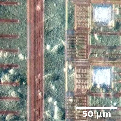
Figure 1: Surface of high-density CMOS MEA. The line shows a scale of 50$\mu$m.

II.2 Method of reconstruction of effective connectivity

We estimate the directed effective connectivity for 8 cases using MEA voltage recordings taken at 8 different Days in Vitro (DIV). In each case, we treat the voltage signal measured by each electrode after noise reduction by a moving average filter (see below) as the activity $x_{i}(t)$ of node $i$, $i=1,2,\ldots,4095$, of a neuronal network Maccione2012 and model the dynamics of the network by a generic system of stochastic differential equations

$$\frac{d{\bf x}}{dt}={\bf F}({\bf x})+{\bf\eta}$$ (1)

where ${\bf x}=(x_{1},x_{2},\ldots,x_{N})$ with $N=4095$, ${\bf F}$ is a general differentiable vector function and $\eta$ is a Gaussian white noise of zero mean and $\overline{\eta_{i}(t)\eta_{j}(t^{\prime})}=D_{ij}\delta(t-t^{\prime})$ that mimics external influences. The overbar denotes an ensemble average over different realizations of the noise. Assuming small fluctuations around the asymptotic noise-free solution ${\bf x}^{*}$, we can linearize the equations to obtain

$$\frac{d\delta x_{i}}{dt}=\sum_{j}w_{ij}\delta x_{j}+\eta_{i},\$$ (2)

where $\delta x_{i}(t)=x_{i}(t)-x^{*}_{i}$ and $w_{ij}\equiv{\partial F_{i}}/{\partial x_{j}}({\bf x}^{*})$ are the elements of ${\bf W}$, which is the Jacobian matrix of ${\bf F}$. When the activity $x_{j}$ affects the time evolution of the activity $x_{i}$, $w_{ij}$ is nonzero and this interaction is represented by a link from node $j$ to node $i$ with a weight $w_{ij}$; otherwise $w_{ij}=0$ and there does not exist a link from node $j$ to node $i$. The HD MEA has a high spatial resolution with the size of each electrode being comparable to the size of a neuron and the cell density in the culture was low such that the voltage measured by an electrode was dominated by the electrical signal of one neuron. Thus we assume that the activity of each node represents contribution mainly from one neuron and the interactions between nodes are through synapses of neurons, and refer the weights of the interactions to as synaptic weights. The effective connectivity is the information of these direct interactions among the different nodes, which are given by the off-diagonal elements of ${\bf W}$. Our goal is to recover the off-diagonal elements $w_{ij}$ with $i\neq j$ from $x_{i}(t)$’s.

We define the elements of the time-lagged covariance matrix ${\bf K}(\tau)$ and the equal-time covariance matrix ${\bf K}(0)$ by

$$K_{ij}(\tau) = \langle[x_{i}(t+\tau)-\langle x_{i}(t+\tau)\rangle][x_{j}(t)-\langle x_{j}(t)\rangle]\rangle\qquad$$ (3)

$$K_{ij}(0) = \langle[x_{i}(t)-\langle x_{i}(t)\rangle][x_{j}(t)-\langle x_{j}(t)\rangle]\rangle.$$ (4)

where $\langle\ldots\rangle$ denotes a time average. For systems that approach a fixed point in the noise-free limit, ${\bf W}$ is time-independent. Then by solving Eq. (2), one obtains Gilson2016 ; ChingTamPRE2017 ; Gustavo ; MasterThesis

$${\bf K}(\tau)=\exp({\tau{\bf W}}){\bf K}(0)$$ (5)

which implies

$$M_{ij}=w_{ij},\qquad{i\neq j}$$ (6)

where

$${\bf M}\equiv\frac{1}{\tau}\log({\bf K}(\tau){\bf K}(0)^{-1})$$ (7)

as long as $\tau$ is not too large ChingTamPRE2017 . Here, $\log$ is the principal matrix logarithm. Equation (5) relates the time-lagged and equal-time covariances ${\bf K}(\tau)$ and ${\bf K}(0)$, which can be calculated using solely the measurements $x_{i}(t)$’s, to ${\bf W}$, which contains information of the direct interactions. The importance of Eq. (6), which follows from Eq. (5), is that the off-diagonal elements $M_{ij}$, $i\neq j$, being approximately equal to $w_{ij}$, should separate into two groups corresponding to $w_{ij}=0$ (no links from node $j$ to node $i$) and $w_{ij}\neq 0$ (links from node $j$ to node $i$ with weights $w_{ij}$). Hence for each node $j$, we can infer $w_{ij}$ by clustering the values of $M_{ij}$ for $i\neq j$ into two groups. As demonstrated by numerical simulations ChingTamPRE2017 ; TamPhDthesis , this covariance-relation based method can recover directed and weighted connectivity not only for the general class of systems as described above but also for some systems that fluctuate around oscillatory dynamics modeled by the FitzHugh-Nagumo dynamics FHN , which is commonly used to model neurons or fluctuate around the chaotic Rössler dynamics Rossler . For these latter systems that do not approach a fixed point in the noise-free limit, the off-diagonal elements of ${\bf W}$ are time-independent and numerical results revealed that Eq. (6) still holds approximately noteW even though Eq. (5) cannot be derived. Motivated by these numerical results, we assume Eq. (6) to hold for some effective time-independent $w_{ij}$’s in our model.

The principal matrix logarithm is very sensitive to noise in measurements and a complex matrix could be resulted when the method is applied to reconstruct realistic systems from experimental measurements. Indeed a complex ${\bf M}$ was obtained when the MEA voltage recordings were directly used in the calculations. Let us denote the voltage signals recorded by the electrodes by $y_{i}(t)$, $i=1,2,\ldots,4095$. We only analyze measurements taken during which all the 4095 electrodes were recording properly. When we calculated ${\bf K}_{y}(\tau)$ and ${\bf K}_{y}(0)$ directly from $y_{i}(t)$ [as defined in Eqs. (3) and (4) with $x_{i}$ replaced by $y_{i}$], we obtained a complex matrix $\log({\bf K}_{y}(\tau){\bf K}_{y}(0)^{-1})$. Similar problem has also been reported in a study of effective connectivity of a cortical network of 68 regions from fMRI recordings and motivated the development of a Lyapunov optimization procedure Gilson2016 . In our study, we are able to avoid this problem by first applying a moving average filter to the voltage signals to reduce the effect of measurement noise. Specifically, we take $x_{i}(t)=[y_{i}(t)+y_{i}(t+\Delta)]/2$, where $\Delta=0.142$ ms is the sampling time interval and calculate ${\bf K}(\tau)$ and ${\bf K}(0)$ using $x_{i}(t)$ with $\tau=\Delta$. The moving average filter is a simple digital low-pass filter that reduces random noise while retaining sharp changes, if any, in the data Smith1999 . The resulting matrix ${\bf M}$ is now real. We have further studied the effect of measurement noise by adding a Gaussian noise to data obtained in numerical simulations of Eq. (1) with $F_{i}=10x_{i}(1-x_{i})+\sum_{j\neq i}w_{ij}(x_{j}-x_{i})$ SunPhDthesis . Our results show that the matrix ${\bf M}$ calculated using the noisy data becomes complex when the standard deviation of the added noise exceeds a certain threshold and a real ${\bf M}$ is restored after the above moving average filter has been applied to the noisy data SunPhDthesis .

After obtaining the real ${\bf M}$, we extend the clustering analysis in Ref. ChingTamPRE2017 , with suitable modifications, to estimate all the off-diagonal elements $w_{ij}$’s of the directed effective connectivity matrix as described below. We assume that the outgoing links of each node, when exist, can only be all excitatory or all inhibitory. To infer the outgoing links of a certain node $j$, we fit the distribution of the values of $M_{ij}$ for all $i\neq j$ by a Gaussian mixture model of two components:

$$P_{\rm fit}(x)= \alpha\frac{1}{\sqrt{2\pi}\sigma_{1}}\exp\left[-\frac{(x-\mu_{1})^{2}}{2\sigma_{1}^{2}}\right]$$ (8)

$$+(1-\alpha)\frac{1}{\sqrt{2\pi}\sigma_{2}}\exp\left[-\frac{(x-\mu_{2})^{2}}{2\sigma_{2}^{2}}\right]$$

This is done by using MATLAB ‘fitgmdist’, which is based on the iterative Expectation-Maximization algorithm MATLAB1 . Two examples of these fits are shown in Fig 2. According to Eq. (6), one expects that the unconnected component of non-existent links of $w_{ij}=0$ should have a mean close to 0 but as can be seen in Fig. 2, the means of the two fitted Gaussian components both deviate from zero. The presence of hidden nodes whose signals are missing can cause a shift in the values of $M_{ij}$’s ChingTamHidden2018 and such hidden nodes could be neural cells lying outside the active electrode area of the MEA probe whose voltage signals were not detected (see Sec. III D). Thus, to improve the performance of our method in the presence of hidden nodes, we make use of the sparsity of the network to identify the unconnected component whenever possible. Specifically, when the two components are well separated with $|\mu_{1}-\mu_{2}|>\sigma_{1}+\sigma_{2}$, we first check whether $\alpha$ or $(1-\alpha)$ is greater than 0.6 and, if yes, identify the component of the larger proportion as the unconnected component corresponding to $w_{ij}=0$. If neither $\alpha$ nor $1-\alpha$ exceeds 0.6, we then take the component whose mean is closer to zero as the unconnected component. The remaining component is referred as the connected component. If the connected component is on the right of the unconnected component as shown in the top panel of Fig 2, then node $j$ is an excitatory node with all outgoing links of $w_{ij}>0$. Otherwise if the connected component is on the left of the unconnected component as shown in the bottom panel of Fig. 2, then node $j$ is an inhibitory node with all outgoing links of $w_{ij}<0$. For each node $j$, the data points $M_{ij}$ for $i\neq j$ are clustered into each of the two components according to the probability $p_{i}$ of each of the $M_{ij}$ values belonging to the unconnected component. We obtain $p_{i}$’s using MATLAB ‘cluster’ which performs agglomerative clustering MATLAB2 . If $p_{i}>0.5$, then $w_{ij}=0$ and there is no link from node $j$ to node $i$. Otherwise if $p_{i}\leq 0.5$, then there is a link from node $j$ to node $i$ with a weight $w_{ij}=M_{ij}-\langle M_{kj}|w_{kj}=0\rangle_{k}$ where $\langle M_{kj}|w_{kj}=0\rangle_{k}$ is the average over $k$ of those $M_{kj}$ values that are estimated to correspond to $w_{kj}=0$. We repeat this procedure for all the nodes $j$ to estimate all the off-diagonal elements $w_{ij}$ with $i\neq j$.

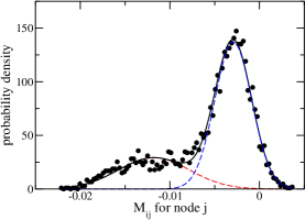
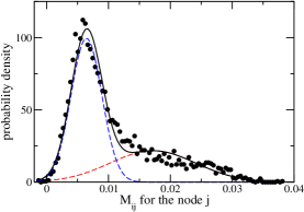
Figure 2: The probability density of $M_{ij}$ for node $j$ (circles). The top panel shows the result for the 4th node ($j=4$) of case 1 and the bottom panel shows the result for the 4076th node ($j=4076$) of case 8. The solid black line is the fit $P_{\rm fit}$ [see Eq. (8)]. The component with a larger relative proportion with $\alpha$ or $1-\alpha$ greater than 0.6 (blue dashed line) is identified as the unconnected component and the other component (red dashed line) is identified as the connected component. In the top panel, the connected component lies on the left of the unconnected component and the node $j$ is inferred as an inhibitory node. In the bottom panel, the connected component lies on the right of the unconnected component and the node $j$ is inferred as an excitatory node.

In the event that the two Gaussian components are not well separated with $|\mu_{1}-\mu_{2}|<{\rm max}(\sigma_{1},\sigma_{2})$, we fit the distribution of $M_{ij}$ again by one single Gaussian distribution, denoted by $P_{G}(x)$ of mean $\mu$. We denote the smooth distribution of $M_{ij}$ estimated using MATLAB ‘ksdensity’, which is based on a normal kernel smoothing function with an optimal bandwidth MATLAB3 , by $P_{K}(x)$. We identify the outliers, which are data points whose values of $P_{K}(x)$ deviate significantly from $P_{G}$, as the connected component with $w_{ij}\neq 0$. Precisely, we define $x_{I}$ and $x_{E}$ by

$$x_{E}=\min_{x>\mu}\{P_{K}(x)=3P_{G}(x)\}$$ (9)

$$x_{I}=\max_{x<\mu}\{P_{K}(x)=3P_{G}(x)\}$$ (10)

then calculate the number of data points in the two groups: (1) $M_{ij}>x_{E}$ and (2) $M_{ij}<x_{I}$ and identify the bigger group of these data points as the connected component with $w_{ij}=M_{ij}-\langle M_{kj}|w_{kj}=0\rangle_{k}$. If no such outliers exist, then node $j$ is inferred to have no detectable outgoing links. For the in-between cases of the two Gaussian components that are neither well separated nor too close to each other with ${\rm max}(\sigma_{1},\sigma_{2})\leq|\mu_{1}-\mu_{2}|\leq\sigma_{1}+\sigma_{2}$, we choose either the two-Gaussian fit or the single-Gaussian fit according to the Bayesian information criterion for fitting models selection Kass1995 ; Raftery1999 .

III Results of the Effective Connectivity

For each of the 8 cases, we study the basic network measures and the distributions of degree and synaptic strength.

III.1 Basic network measures

We calculate several basic network measures including the connection probability $p$, the ratio $r_{B}$ of the number of bidirectionally connected pairs to the expected number for a random network with same connection probability $p$, the fractions $f_{E}$ and $f_{I}$ of excitatory and inhibitory nodes, the fraction $f_{\rm SCC}$ of nodes that form the strongly connected component, the characteristic path length $l$, the average clustering coefficient (CC) and the small world index (SWI). The results are shown in Table 1. The connection probability $p$ of a network of $N$ nodes with $N_{L}$ links is defined by $p=N_{L}/[N(N-1)]$. We find that $p$ ranges from 0.7-1.9% which is consistent with our assumption that the neuronal networks are sparse. This average value of $p$ is smaller but comparable to that of the chemical synapse network of C. elegans Varshney2011 . Most of the connections are unidirectional in accord with the directional transmission of signals in neurons. One expects neuronal networks to be organized and thus highly nonrandom in order to facilitate effective and efficient signal transmission. For a random network of $n$ nodes and connection probability $p$, the expected number of bidirectionally connected pairs is given by $N(N-1)p^{2}/2$. We denote the ratio of the number of bidirectionally connected pairs in the network to the expected number in a random network by $r_{B}$. The values of $r_{B}$ exceed 4 for all the networks, consistent with the well-documented over-representation of bidirectional connected pairs in rat cortical circuits SongPLoS2005 ; MarkramJPhysio1997 ; SjostromNeuron2001 ; PerinPNAS2011 .

	case 1	case 2	case 3	case 4	case 5	case 6	case 7	case 8	C. elegans
DIV	11	22	25	33	45	52	59	66	—
$p$ (%)	1.2	1.9	1.4	1.5	1.1	1.7	1.4	1.5	2.8
$r_{B}$	5.9	5.5	10.7	5.7	6.5	4.21	4.0	4.4	—
$f_{E}$	0.62	0.80	0.84	0.75	0.62	0.66	0.48	0.57	—
$f_{I}$	0.27	0.13	0.14	0.18	0.21	0.24	0.32	0.28	—
$f_{\rm SCC}$	0.88	0.93	0.98	0.92	0.81	0.90	0.77	0.83	0.85
$l$	4.0	3.7	3.7	3.9	4.1	3.7	3.8	3.8	3.5
CC	0.26	0.36	0.38	0.30	0.25	0.28	0.18	0.22	0.22
SWI	13.1	11.3	17.1	12.7	14.4	10.4	7.9	8.8	2.3

Table 1: Basic network measures of the networks reconstructed. When available, the corresponding results for the chemical synapse network of C. elegans Varshney2011 are included for comparison.

Each node is inferred as excitatory or inhibitory according to the sign of the synaptic weights of its outgoing links as discussed in Sec. II. There is a small fraction of nodes with no detectable outgoing links. As can be seen in Table 1, the values of $f_{I}$ range from 0.13 to 0.31, which are comparable to the measured fractions (0.15-0.30) of inhibitory neurons in various cortical regions in monkey Hendry1987 . The balance between excitation and inhibition in the cortex is believed to play an important role in executing proper brain functions and disruption of such a balance may underlie the behavioral deficits that are observed in conditions such as autism and schizophrenia Rubenstein2003 ; Levitt2004 ; Yizhar2011 ; Lewis2011 ; Marin2012 . The fraction $f_{\rm SCC}$ of nodes that form the largest strongly connected component exceeds 70% for all the cases studied. The characteristic path length $l$, which is the average shortest path length for all nodes that can be connected by a finite path is about 4, and the average local clustering coefficient CC, which is the average of the connection probability of the outgoing neighbors of each node, ranges from $0.18-0.38$. These network properties are comparable to those of the chemical synapse network of C. elegans. Furthermore, the reconstructed neuronal networks all have small-world topology, with small-world index SWI substantially greater than one. It has been shown that small-world networks allow efficient transmission of information LatoraPRL2001 .

III.2 Distributions of incoming and outgoing degrees

The distributions of the incoming and outgoing degrees are qualitatively the same for all the 8 cases and results for one case are shown in Fig. 3. There are several notable features. First, most of the nodes have a small $k_{\rm out}$ that is less than a few tens but a small fraction of nodes have an exceptionally large $k_{\rm out}$ exceeding a thousand. This is the case for both the excitatory and inhibitory nodes. Second, the incoming degree distribution is approximately bimodal, which is different from the approximate scale-free distribution reported for functional connectivity Pastore2018  (see also Sec. IV). The bimodal feature of the incoming degree distribution is more clearly revealed in the separate distributions of the excitatory and inhibitory incoming degrees $k_{\rm in}^{+}$ and $k_{\rm in}^{-}$ for incoming links of positive and negative synaptic $w_{ij}$, respectively (see Fig. 4). By studying the distribution of $k_{\rm in}^{+}$ (or $k_{\rm in}^{-}$) separately for the two modes of nodes of small and large $k_{\rm in}^{-}$ ($k_{\rm in}^{+}$) (see inset of Fig. 4), it can be seen that nodes tend not to have both large $k_{\rm in}^{+}$ and large $k_{\rm in}^{-}$.

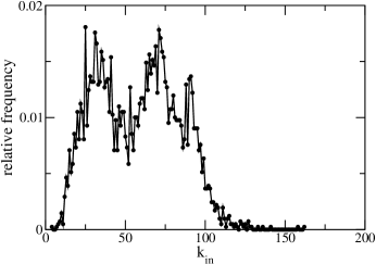
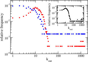
Figure 3: Distributions of the incoming degree $k_{\rm in}$ (top panel) and outgoing degree $k_{\rm out}$ (bottom panel) of case 3. In the bottom panel, we show the distribution of $k_{\rm out}$ separately for excitatory (circles) and inhibitory nodes (squares) and for all the nodes in the inset.

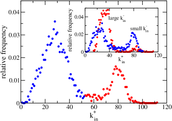
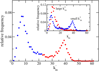
Figure 4: Distributions of the excitatory and inhibitory incoming degrees, $k_{\rm in}^{+}$ (top panel) and $k_{\rm in}^{-}$ (bottom panel), of case 3. The distributions are clearly bimodal with two modes of large and small $k_{\rm in}^{+}$ or $k_{\rm in}^{-}$. In the insets, we show the relative frequencies separately for the two modes of nodes of small and large $k_{\rm in}^{-}$ (or $k_{\rm in}^{+}$).

III.3 Distributions of average synaptic strength

Both in vitro and in vivo studies have indicated that the distribution of synaptic weights in the cortex are generally skewed with long tails and typically lognormal Buzsaki2014 . Motivated by these findings, we study the distributions of the average synaptic strength of the links. The various averages of the synaptic weights are defined as follows

$$s_{\rm in}(i) \equiv \frac{\sum_{j\neq i}w_{ij}}{k_{in}(i)}$$ (11)

$$s_{\rm in}^{+}(i) \equiv \frac{\sum_{j\neq i,w_{ij}>0}w_{ij}}{k_{\rm in}^{+}(i)}$$ (12)

$$s_{\rm in}^{-}(i) \equiv \frac{\sum_{j\neq i,w_{ij}<0}w_{ij}}{k_{\rm in}^{-}(i)}$$ (13)

$$s_{\rm out}(i) \equiv \frac{\sum_{j\neq i}w_{ji}}{k_{\rm out}(i)}.$$ (14)

Among these quantities, $s_{\rm in}^{+}\geq 0$ is the average of the synaptic weights of excitatory incoming links and $s_{\rm in}^{-}\leq 0$ is the average of the synaptic weights of inhibitory incoming links, $s_{\rm in}$ is the average of the synaptic weights of all incoming links and can be positive or negative, and $s_{\rm out}$ is the average of the synaptic weights of all outgoing links and is positive for excitatory nodes, negative for inhibitory nodes and zero for the nodes with no detectable outgoing links. To have better statistics, we use the data from all the 8 networks to calculate the distributions. We first calculate the mean and standard deviation of these average synaptic weights in each of the networks and then calculate the distribution of the standardized values, which are the values subtracted by the mean and divided by the standard deviation. The distribution of $s_{\rm out}$ for excitatory nodes is found to depend on whether $s_{\rm in}$ is positive or negative. As seen in Fig 5, all these average synaptic strengths have a non-Gaussian distribution that is skewed with long tails. This indicates that a small fraction of the nodes have dominantly strong average synaptic strengths and thus the average synaptic strength of the links of the nodes are not well represented by the mean values. We also calculate the distribution of the standardized values of the logarithm of these average synaptic strengths and find that $s_{\rm out}$ for excitatory nodes with $s_{\rm in}>0$ has an approximately lognormal distribution (see Fig. 5).

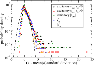
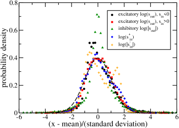
Figure 5: Distributions of the average synaptic strengths of excitatory and inhibitory incoming links $s_{\rm in}^{+}$ and $s_{\rm in}^{-}$ and of outgoing links $s_{\rm out}$. Top panel: Distributions of the standardized values of the average synaptic strength, $(x-{\rm mean})/(\mbox{standard deviation})$, where $x$ is $s_{\rm in}^{+}$, $s_{\rm in}^{-}$ or $s_{\rm out}$ in each case. Bottom panel: Distributions of the standardized values of the logarithm of the average synaptic weights with $x$ now being $\log(s_{\rm in}^{+})$, $\log(|s_{\rm in}^{-}|)$ or $\log(|s_{\rm out}|)$. The dashed line is the standardized Gaussian distribution.

III.4 Possible effects of hidden nodes

Neural cells lying in the working area outside the active electrode area of the MEA probe could form synaptic connections with cells within the active electrode area but their spontaneous activities were not recorded. Thus the MEA recordings could miss out information from those nodes that were not detected. These nodes are thus the so-called hidden nodes. It has been shown that in bidirectional networks the presence of hidden nodes that are randomly missed out has no significant adverse effects on the reconstruction of the links among the measured nodes ChingTamHidden2018 . To investigate whether and how undetected signals from the hidden nodes might affect our results, we reconstruct a partial network using only recordings of 2025 electrodes, which are the 45 by 45 electrodes in the central region of the active electrode area, and compare it with the subnetwork of these corresponding 2025 nodes, extracted from the whole network that we reconstructed using recordings of all the 4095 electrodes for case 3. We find that the partial network captures correctly 99.8% of the non-existent links and 83.0% of the links in the subnetwork. Moreover, the partial network and the subnetwork have similar in- and out-degree distributions as shown in Fig. 6. These results support that the directed effective connectivity obtained using the 4095 electrodes is not significantly affected by the possibly missed out signals from the neural cells lying outside the active electrode area of the MEA probe.

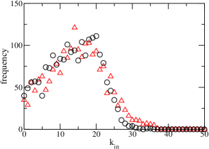
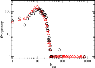
Figure 6: Distributions of in- and out-degrees of the subnetwork (circles) and partial network (triangles) for case 3.

IV Comparison of Effective Connectivity and Functional Connectivity

The effective connectivity studied in the present work is proposed to capture the direct interactions among the nodes based on the general class of model described in Eq. (1) while functional connectivity studied in existing methods is based mainly on the statistical dependence of the dynamics of the nodes. It is thus expected that effective connectivity and functional connectivity to contain different information about the system. In this Section, we compare directly the two types of connectivity estimated from the same sets of measurements. We follow the method in Ref. Pastore2018 to estimate the functional connectivity using the statistical correlation of the spikes detected from the MEA recordings. By applying the Precise Timing Spike Detection algorithm PTSD in the BrainWave software to the recorded time series $y_{i}(t)$ of the $i$-th electrode, we obtain the times of the spikes $t^{(i)}_{k}$, $k=1,2,\ldots,N_{i}$, for the $N_{i}$ spikes detected for node $i$. The spike train $S_{i}(t)$ is constructed as follows: $S_{i}(t)=1$ for $t=t^{(i)}_{k}$, $k=1,2,\ldots,N_{i}$ and $0$ otherwise. The general idea is to estimate a functional link between nodes $i$ and $j$ when the correlation between the two spike trains exceeds a certain threshold. The cross-correlation of the spiking activity of nodes $i$ and $j$ is measured by $C_{ij}\in[0,1]$, which is defined by Maccione2012

$$C_{ij}(\tau)=\frac{1}{\sqrt{N_{i}N_{j}}}\sum_{k=1}^{N_{i}}S_{i}(t^{(i)}_{k})S_{j}(t^{(i)}_{k}+\tau)$$ (15)

In the earlier method Maccione2012 , $C_{ij}(\tau)$ is calculated in a window of $\tau$-values: $-n\Delta\leq\tau\leq n\Delta$, where $\Delta$ is the sampling time interval and if the maximum value $C_{ij}(\tau_{0})$ at $\tau_{0}$ within this window exceeds a certain threshold then a link of weight $C_{ij}(\tau_{0})$ is inferred between nodes $i$ and $j$ with the direction of the link determined by the sign of $\tau_{0}$. To detect also inhibitory links with negative weights, $f_{ij}(\tau)$ measuring the difference of $C_{ij}(\tau)$ from its average value in the window has been introduced Pastore2018

$$f_{ij}(\tau)=C_{ij}(\tau)-\frac{1}{2n+1}\sum_{k=-n}^{n}C_{ij}(k\Delta),$$ (16)

which can assume both positive and negative values. In our calculations, we use $n=100$. Let $|f_{ij}(\tau)|$ attain its maximum at $\tau=\tau^{*}$ note ; a link is inferred for the functional connectivity, from node $i$ to node $j$ if $\tau^{*}>0$ and from node $j$ to node $i$ if $\tau^{*}<0$, with strength $f_{ij}(\tau^{*})$ when $|f_{ij}(\tau^{*})|$ exceeds a certain threshold and $|\tau^{*}|$ is not shorter than the time needed for a synaptic signal with a propagation speed of 400mm/s Pastore2018 . Excitatory links have $f_{ij}(\tau^{*})>0$ while inhibitory links have $f_{ij}(\tau^{*})<0$. The requirement that a node is either excitatory or inhibitory, with outgoing links having only one sign, cannot be enforced in this cross-correlation based method for estimating functional connectivity. This method also has a considerably weaker sensitivity for detecting inhibitory links Pastore2018 . In contrast, the covariance-relation based method that we use to estimate effective connectivity can detect excitatory and inhibitory links equally well using only a recording time of 5 minutes.

Comparing to effective connectivity, a large fraction (0.2 to 0.46) of nodes have zero incoming or outgoing degrees in the estimated functional connectivity. In Fig. 7, we show the distributions of nonzero incoming and outgoing degrees for functional connectivity. It can be seen that the two distributions are similar and are clearly different than the incoming and outgoing degree distributions found in effective connectivity (see Fig. 3). The degree distribution in functional connectivity estimated from measurements recorded in a much longer duration of one hour has been found to be scale-free Pastore2018 . We compare the strongest excitatory and inhibitory links estimated in the two types of connectivity in Fig. 8. We choose 200 strongest excitatory links and 50 strongest inhibitory links in the effective connectivity. It is not possible to choose exactly the same number of links in functional connectivity as many links have the same coupling strength and we choose the closest number of links for the comparison. In the effective connectivity, most of the strongest excitatory links are connecting nearby nodes. This feature is not found in the functional connectivity.

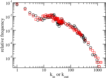
Figure 7: Distributions of the incoming and outgoing degree, $k_{\rm in}$ (circles) and $k_{\rm out}$ (squares) of the functional connectivity estimated for case 3.

Figure 8: Comparison of the strongest $N_{\rm exc}$ excitatory (red) and the strongest $N_{\rm inh}$ inhibitory links (blue) of the effective connectivity (top panels) and of the functional connectivity (bottom panels) for case 3. $N_{\rm inh}=50$ for both types of connectivity, $N_{\rm exc}=200$ for effective connectivity and $N_{\rm exc}=151$ for functional connectivity.

To check whether the proposed effective connectivity can indeed reveal relationships between network structure and dynamics better than functional connectivity, we study the relation between the spiking activity and the average synaptic strength of the nodes. Specifically, we divide the nodes into several groups according to their number of detected spikes and calculate the mean values of the average synaptic strength of excitatory and inhibitory incoming and outgoing links of these different groups. Since nodes have both excitatory and inhibitory outgoing links in the estimated functional connectivity, we generalize the definition of $s_{\rm out}$ to $s_{\rm out}^{+}$ and $s_{\rm out}^{-}$:

$$s_{\rm out}^{+}(i) \equiv \frac{\sum_{j\neq i,w_{ji}>0}w_{ji}}{k_{\rm out}^{+}(i)},$$ (17)

$$s_{\rm out}^{-}(i) \equiv \frac{\sum_{j\neq i,w_{ji}<0}w_{ji}}{k_{\rm out}^{-}(i)},$$ (18)

and $s_{\rm out}^{+}$ ($s_{\rm out}^{-}$) is equal to zero for nodes without excitatory (inhibitory) outgoing links. For the effective connectivity, $s_{\rm out}^{+}$ ($s_{\rm out}^{-}$) is equal to $s_{\rm out}$ for excitatory (inhibitory) nodes. The results for the two types of connectivity are shown in Figs. 9 and 10. The dependence of the mean values of $s_{\rm in}^{-}$ and $s_{\rm out}^{-}$ on the spiking activity is weak for both types of connectivity. Definite dependencies of the mean values of $s_{\rm in}^{+}$ and $s_{\rm out}^{+}$ on the number of detected spikes are found in our estimated effective connectivity but not in the estimated functional connectivity. In particular, the intuition that nodes with larger $s_{\rm in}^{+}$ would spike more is supported by the effective connectivity but not functional connectivity. The effective connectivity further reveals that nodes spike more have larger $s_{\rm out}^{+}$ on average and such a definite dependence is again lacking in the functional connectivity.

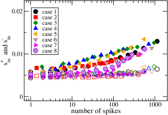
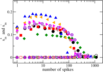
Figure 9: The dependence of the mean values of $s_{\rm in}^{+}$ and $s_{\rm in}^{-}$ on the number of detected spikes of the nodes in effective connectivity (top panel) and functional connectivity (bottom panel). The filled and shaded symbols shown in the legend denote $s_{\rm in}^{+}$ and $s_{\rm in}^{-}$ are denoted by the corresponding open symbols for cases 1-7 and by the star symbols for case 8.

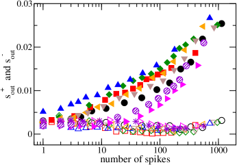
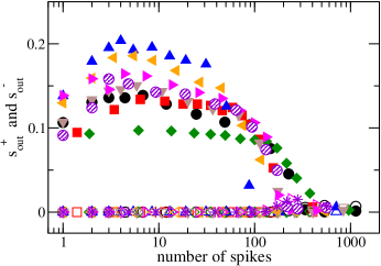
Figure 10: The dependence of the mean values of $s_{\rm out}^{+}$ and $s_{\rm out}^{-}$ on the number of detected spikes of the nodes in effective connectivity (top panel) and functional connectivity (bottom panel). Same symbols as in Fig. 9

.

V Summary and Conclusions

Revealing connectivity of neuronal networks from measurements taken by large-scale MEA is a challenging inverse problem. Existing methods focus on functional connectivity that is based on the statistical correlation of the detected spiking activities. As statistical correlation arising from indirect influences lead to false positives, efforts have been spent to optimize the performance of inference based on spike cross-correlation. In a recent study Kobayashi2019 , a method, denoted as GLMCC, has been developed by applying a generalized linear model to spike cross-correlations which shows how an increase of the duration of spike recording can improve the performance of inference. This study further gives an analytical estimate of the required duration for reliable inference which is inversely related to the firing rates of the neurons and the synaptic strength of the connections. In our work, we study effective connectivity, which measures direct interactions and should be more relevant and useful for studying the relationships between network structure and dynamics and between network structure and functions of neuronal networks. We have modelled in vitro neuronal cultures as stochastic dynamical systems and adopted a general method that reconstructs directed links and their relative weights of a network from dynamics ChingTamPRE2017 to estimate effective connectivity of neuronal cultures from voltage measurements recorded by MEA. This general method makes use of Eq. (6), which follows from Eq. (5), a relation between the time-lagged covariance and the equal-time covariance of the dynamics to extract information of the direct interactions of the nodes. Equation (5) is derived for systems that approach a fixed point in the noise-free limit and numerical results revealed that Eq. (6) also holds approximately for systems that fluctuate around oscillatory FitzHugh-Nagumo dynamics or chaotic Rossler dynamics PhysicaA2018 ; ChingTamPRE2017 ; TamPhDthesis even though Eq. (5) cannot be derived. Motivated by these numerical results, we assume Eq. (6) to hold for our model. For networks of stochastic binary neurons with activity being either 0 or 1, a relation between the time-lagged covariance and equal-time covariance similar to Eq. (5) can be obtained RoudiPRL2011 ; Mezard2011 ; Frontiers2013 ; PRX2016 and used to reconstruct the effective synaptic couplings of the neurons PRX2016 . In our model, the activity of each neuron is described by the continuous variable $x_{i}(t)$ and the time-lagged and equal-time covariances are calculated using the whole time series of the voltage measurements and not only the spike trains of 0’s and 1’s. When applying this method to reconstruct real network from experimental measurements, we have to overcome additional difficulties. One major difficulty is that this involves a calculation of a principal matrix logarithm, which is very sensitive to noise in the data. If the method is applied directly to the MEA voltage recordings, a complex matrix would be obtained. By first applying a moving average filter to the MEA voltage recordings to reduce the effect of noise, the problem of complex matrix has been avoided and we have successfully estimated the effective connectivity, namely the directed interactions with their synaptic weights, of neuronal networks of over 4000 nodes from relatively short MEA recordings of 5 min. In comparison, good performance of the GLMCC method has been shown using numerical data with a much longer duration of 90 min of spike recording Kobayashi2019 . Moreover, as our method makes use of the whole voltage time series and not only the detected spikes, low firing rates in the MEA recording do not pose an additional difficulty.

Our results of the effective connectivity reproduce various reported features of cortical regions in rats and monkeys and has similar network properties as the nematode C. elegans chemical synaptic network, supporting that the estimated effective connectivity can capture the general properties of synaptic connections. Moreover, numerical simulations of networks of spiking neurons using the estimated effective connectivity reproduce the long-tailed distribution of firing rates found in the MEA recordings Frontiers . The distributions of incoming and outgoing degrees are different from the reported scale-free distributions in the functional connectivity Pastore2018 . In particular the excitatory and inhibitory incoming degree distributions are found to be bimodal. There have been studies indicating that the robustness of undirected networks against both random failures and targeted attacks can be optimized by having a bimodal degree distribution Stone2004 ; Stanley2005 and future studies are required to establish the significance of the bimodal feature of incoming degree distributions. We have found that the distributions of average synaptic strengths are non-Gaussian and skewed with a long tail and that the distribution of the average synaptic strength of outgoing links for excitatory nodes with positive average synaptic strength of incoming links ($s_{\rm in}>0$) is approximately lognormal, and our results are consistent with reported results found in in vitro and in vivo studies of synaptic strengths in the cortex Buzsaki2014 . The significance of such non-Gaussian distributions with long tails is that a small fraction of nodes have dominantly strong average synaptic strength suggesting the possibility that the bulk of the information flow occurring mostly through them Buzsaki2014 . It would be interesting to understand how the long-tailed synaptic strength distribution might be related to the spiking and bursting dynamics.

The effective connectivity and functional connectivity estimated from the same sets of MEA recordings are different. The average synaptic strengths of excitatory incoming and outgoing links are found to increase with the spiking activity in the estimated effective connectivity but not in the estimated functional connectivity. These findings demonstrate that the effective connectivity estimated in the present work can indeed better reveal relationships between network structure and dynamics for neuronal cultures. Understanding the relationships between network structure and dynamics will be a topic of interest in future studies.

*

Appendix: Experimental details on the neuronal culture

The complementary metal-oxide-semiconductor (CMOS)-based high density multielectrode array (HD-MEA) was pre-coated with 0.1 % Poly-D-lysine (Sigma P6407) and 0.1 % adhesion proteins laminin (Sigma L2020). After plating on the HD-MEA chip, cultures were filled with 1 ml of culture medium [DMEM (Gibco 10569) + 5% FBS (Gibco 26140) + 5% HS (Gibco 16050) + 1% PS (Gibco 15140)] and placed in a humidified incubator (5% CO₂, 37^∘C). Half of the medium was replaced by Neurobasal medium supplemented with B27 [Neurobasel medium (Gibco. 21103) + 2% 50X B27 supplement (Gibco. 17504) + 200 $\mu M$ GlutaMAX (Gibco 35050)] twice a week.

References

- (1) S.H. Strogatz, Exploring complex networks, Nature (London) 410, 268 (2001).
- (2) R. Albert and A.-L. Barabási, Statistical mechanics of complex networks, Rev. Mod. Phys. 74, 48 (2002).
- (3) M.E.J. Newman, The Structure and Function of Complex Networks, SIAM Rev. 45, 167 (2003).
- (4) E. Bullmore and O. Sporns, Complex brain networks: graph theoretical analysis of structural and functional systems, Nat. Rev. Neurosci. 10, 186 (2009)
- (5) D.S. Bassett and O. Sporns, Network neuroscience, Nat. Neurosci. 20, 353 (2017).
- (6) K.J. Friston, Functional and Effective Connectivity: A Review, Brain Connectivity 1, 13-36 (2011).
- (7) O. Sporns, Networks of the Brain, MIT Press (2011).
- (8) J.P. Eckmann, O. Feinerman, L. Gruendinger, E. Moses, J. Soriano and T. Tlusty, The physics of living neural networks, Phys. Rep. 449, 54 (2007).
- (9) O. Feinerman, A. Rotem and E. Moses, Reliable neuronal logic devices from patterned hippocampal cultures, Nat. Phys. 4, 967 (2008).
- (10) J. Soriano, J. Casademunt, Neuronal cultures: The brain’s complexity and non-equilibrium physics, all in a dish, Contrib. Sci. 11, 225 (2015).
- (11) M.E.J. Obien, K. Deligkaris, T. Bullmann, D.J. Bakkum and U. Frey, Revealing neuronal function through microelectrode array recordings, Front. Neurosci. 8, 423 (2015).
- (12) A. Maccoine, N. Garofalo, T. Nieus, M. Tedesco, L. Berdondini and S. Martinoia, Multiscale functional connectivity estimation on low-density neuronal cultures recorded by high-density CMOS Micro Electrode Arrays, J. NeuroSci. Methods 207, 161-171 (2012).
- (13) D. Poli, V.P. Pastore, and P. Massobrio, Functional connectivity in in vitro neuronal assemblies, Front. Neural Circuits 9, 57 (2015).
- (14) V.P. Pastore, P. Massobrio, A. Godjoski, S. Martinoia, Identification of excitatory-inhibitory links and network topology in large-scale neuronal assemblies from multi-electrode recordings, PLoS Comput. Biol. 14, e1006381 (2018).
- (15) L.M.A. Bettencourt, G.J. Stephens, M.I. Ham and G.W. Gross, Functional structure of cortical neuronal networks grown in vitro, Phys. Rev. E 75, 021915 (2007).
- (16) L.M.A. Bettencourt, V. Gintautas and M.I. Ham, Identification of Functional Information Subgraphs in Complex Networks, Phys. Rev. Lett. 100, 238701 (2008).
- (17) M. Timme and J. Casadiego, Revealing networks from dynamics: an introduction, J. Phys. A: Math. Theor. 47, 343001 (2014).
- (18) M. Gilson, R. Moreno-Bote, A. Ponce-Alvarez, P. Ritter and G. Deco, Estimation of Directed Effective Connectivity from fMRI Functional Connectivity Hints at Asymmetries of Cortical Connectome, PLoS Comput. Biol. 12, e1004762 (2016).
- (19) H.C. Tam, E.S.C. Ching and P.Y. Lai, Reconstructed networks from dynamics with correlated noise, Physica A 502, 106-122 (2018).
- (20) J. Ren, W.-X. Wang, B. Li, and Y.-C. Lai, Noise Bridges Dynamical Correlation and Topology in Coupled Oscillator Networks, Phys. Rev. Lett. 104, 058701 (2010).
- (21) E.S.C. Ching, P.Y. Lai and C.Y. Leung, Extracting connectivity from dynamics of networks with uniform bidirectional coupling, Phys. Rev. E 88, 042817 (2013); Erratum, Phys. Rev. E 89, 029901(E) (2014).
- (22) E.S.C. Ching, P.Y. Lai and C.Y. Leung, Reconstructing Weighted Networks from Dynamics, Phys. Rev. E 91, 030801(R) (2015).
- (23) E. Schneidman, M.J. Berry, R. Segev and W. Bialek, Weak pairwise correlations imply strongly correlated network states in a neural population, Nature 440, 1007 (2006).
- (24) M. K. S. Yeung, J. Tegnér, and J. J. Collins, Reverse engineering gene networks using singular value decomposition and robust regression, Proc. Natl. Acad. Sci. U.S.A. 99, 6163 (2002).
- (25) D. Napoletani and T. D. Sauer, Reconstructing the topology of sparsely connected dynamical networks, Phys. Rev. E 77, 026103 (2008).
- (26) D. Yu, M. Righero, and L. Kocarev, Estimating Topology of Networks, Phys. Rev. Lett. 97, 188701 (2006).
- (27) S. G. Shandilya and M. Timme, Inferring network topolgy from complex dynamics, New J. of Phys. 13, 013004 (2011).
- (28) Z. Levnajić and A. Pikovsky, Network Reconstruction from Random Phase Resetting, Phys. Rev. Let. 107, 034101 (2011).
- (29) S. Shahrampour and V. M. Preciado, Reconstruction of Directed Networks from Consensus Dynamics, American Control Conference, 1685 (2013).
- (30) Z. Levnajić and A. Pikovsky, Untangling complex dynamical systems via derivative-variable correlations, Sci. Rep. 4, 5030 (2014).
- (31) T. S. Gardner, D. di Bernardo, D. Lorenz, and J. J. Collins, Inferring Genetic Networks and Identifying Compound Mode of Action via Expression Profiling, Science 301, 102 (2003).
- (32) K. J. Friston, L. Harrison and W. Penny, Dynamic casual modelling, NeuroImage 19, 1273 (2003).
- (33) M. Timme, Revealing Network Connectivity from Response Dynamics, Phys. Rev. Lett. 98, 224101 (2007).
- (34) J. Casadiego, M. Nitzan, S. Hallerberg and M. Timme, Model-free inference of direct network interactions from nonlinear collective dynamics, Nat. Commun. 8, 2192 (2017).
- (35) R. J. Prill, R. Vogel, G. A. Cecchi, G. Altan-Bonnet and G. Stolovitzky, Noise-Driven Causal Inference in Biomolecular Networks, PLoS ONE 10, e0125777 (2015).
- (36) B. J. Lüsmann, Reconstruction of Physical Interactions in Stationary Stochastic Network Dynamics, Master Thesis, Max Planck Inst. for Dynamics and Self-Organization (2015).
- (37) E. S. C. Ching and H. C. Tam, Reconstructing links in directed networks from noisy dynamics, Phys. Rev. E 95, 010301(R) (2017).
- (38) P. Y. Lai, Reconstructing Network topology and coupling strengths in Directed Networks of discrete-time dynamics, Phys. Rev. E 95, 022311 (2017).
- (39) B. J. Lüsmann, C. Kirst and M. Timme, Transition to reconstructibility in weakly coupled networks, PLoS ONE 12, e0186624 (2017).
- (40) H. C. Tam, Reconstruction of Networks from Noisy Dynamics, Ph.D. Thesis, The Chinese University of Hong Kong (2017).
- (41) R. FitzHugh, Impulses and physiological states in theoretical models of nerve membrane, Biophys. J. 1, 445 (1961).
- (42) O. E. Rössler, An Equation for Continuous Chaos, Phys. Lett. A 57, 397 (1976).
- (43) In these systems, each node has more than one state variable (two for systems with FitzHugh Nagmumo dynamics and three for systems with Rössler dynamics) and only one state variable is acted upon by the noise directly and the matrix is calculated using the time series of this state variable.
- (44) S. W. Smith, The Scientist and Engineer’s Guide to Digital Signal Processing. 2nd ed. San Diego: California Technical Publishing; 1999.
- (45) Chumin Sun, Reconstruction and Analysis of the Directed Effective Connectivity of Neuronal Networks, Ph.D. Thesis, The Chinese University of Hong Kong (2020).
- (46) A.P. Dempster, N.M. Laird and D.B. Rubin, Maximum Likelihood from Incomplete Data via the EM Algorithm, J. of the Royal Statistical Society, Series B 39, 1 (1977).
- (47) E.S.C. Ching and P.H. Tam, Effects of hidden nodes on the reconstruction of bidirectional networks, Phys. Rev. E 98, 062318 (2018).
- (48) A. Maccione, M. Gandolfo, P. Massobrio, A. Novellino, S. Martinoia and M. Chiappalone, A novel algorithm for precise identification of spikes in extracellularly recorded neuronal signals, J. Neurosci. Methods 177, 241 (2009).
- (49) Frank Nielsen, Introduction to HPC with MPI for Data Science, p. 195, , (Springer 2016).
- (50) B.W. Silverman, Density Estimation for Statistics and Data Analysis, (Chapman & Hall, London 1986).
- (51) R.E. Kass, A.E. Raftery, Bayes factors, J. Amer. Stat. Assoc. 90, 773-795 (1995).
- (52) A.E. Raftery, Bayes factors and BIC: Comment on a critique of the Bayesian information criterion for model selection, Sociol. Methods Res. 27, 411-427 (1999).
- (53) L.R. Varshney, B.L. Chen, E. Paniagua, D.H. Hall and R.B. Chklovskii, Structural Properties of the Caenorhabditis elegans Neuronal Network, PLoS Comput. Biol. 7, e1001066 (2011).
- (54) S. Song, P.J. Sjöström, M. Reigl, S. Nelson and R.B. Chklovskii, Highly Nonrandom Features of Synaptic Connectivity in Local Cortical Circuits, PLoS Biology 3, e350 (2005).
- (55) H. Markram, J. Lübke, M. Frotscher, A. Roth and B. Sakmann, Physiology and anatomy of synaptic connections between thick tufted pyramidal neurones in the developing rat neocortex, J. Physio. 500, 409-440 (1997).
- (56) P.J. Sjöström, G.G. Turrigiano and S.B. Nelson, Rate, timing, and cooperativity jointly determine cortical synaptic plasticity, Neuron 32, 1149-1164 (2001).
- (57) R. Perin, T.K. Berger and H. Markram, A synaptic organizing principle for cortical neuronal groups, PNAS 108, 5419-5425 (2001).
- (58) S.H. Hendry, H.D. Schwark, E.G. Jones and J. Yan, Numbers and proportions of GABA-immunoreactive neurons in different areas of monkey cerebral cortex, J. Neurosci. 7, 1503-1519 (1987).
- (59) J.L. Rubenstein and M.M. Merzenich, Model of autism: increased ratio of excitation/inhibition in key neural systems, Genes Brain Behav. 2, 255-67 (2003).
- (60) P. Levitt, K.L. Eagleson and E.M. Powell, Regulation of neocortical interneuron development and the implications for neurodevelopmental disorders, Trends Neurosci. 27, 400-6 (2004).
- (61) O. Yizhar, L.E. Fenno, M. Prigge, F. Schneider, T.J. Davidson, D.J. O’Shea et al., Neocortical excitation/inhibition balance in information processing and social dysfunction, Nature 477, 171-178 (2011).
- (62) D.A. Lewis, K.N. Fish, D. Arion and G. Gonzalez-Burgos, Perisomatic inhibition and cortical circuit dysfunction in schizophrenia, Curr. Opin. Neurobiol. 21, 866-72 (2011).
- (63) O. Marin, Interneuron dysfunction in psychiatric disorders. Nat. Rev. Neurosci. 13, 107-20 (2012).
- (64) V. Latora and M. Marchori, Efficient Behavior of Small-World Networks, Phys. Rev. Lett. 87, 198701 (2001).
- (65) G. Buzsaki and K. Mizuseki, The log-dynamic brain: how skewed distributions affect network operations, Nat. Neurosci. 15, 264-278 (2014).
- (66) When attains its maximum at more than one value of , all of the same sign, is taken as the -value with the minimum magnitude. If the values of at which attains its maximum include both positive and negative values, then we take as the -value with the minimum magnitude separately for the positive and negative -values. If these two both satisfy the criterion set by the maximum propagation speed of synaptic signal, then there are bidirectional links between nodes and with the same coupling strength in either direction.
- (67) A.X.C.N. Valente, A. Sarkar, H.A. Stone, Two-peak and three-peak optimal complex networks, Phys. Rev. Lett. 92, 118702 (2004).
- (68) T. Tanizawa, G. Paul, R. Cohen, S. Havlin and H.E. Stanley, Optimization of network robustness to waves of targeted and random attacks, Phys. Rev. E 71, 047101 (2005).
- (69) R. Kobayashi, S. Kurita, A. Kurth, K. Kitano, K. Mizuseki, M. Diesmann, B. J. Richmond and S. Shinomoto, Reconstructing neuronal circuitry from parallel spike trains, Nat. Commun. 10, 4468 (2019).
- (70) Y. Roudi and J. Hertz, Mean Field Theory for Nonequilibrium Network Reconstruction, Phys. Rev. Lett. 106, 048702 (2011).
- (71) M. Mézard and J. Sakellariou, Exact Mean-Field Inference in Asymmetric Kinetic Ising Systems, J. Stat. Mech. L07001 (2011).
- (72) D. Grystskyy, T. Tetzlaff, M. Diesmann and M. Helias, A unified view on wealy correlated recurrent networks, Front. Comp. Neurosci. 7, 131 (2013).
- (73) D. Dahmen, H. Bos, and M. Helias, Correlated Fluctuations in Strongly Coupled Binary Networks Beyond Equilibrium, Phys. Rev. X 6, 031024 (2016).
- (74) H. Y. Li, G. M. Cheng and E. S. C. Ching, Heterogeneous Responses to Changes in Inhibitory Synaptic Strength in Networks of Spiking Neurons, Front. Cell. Neurosci. 16, 785207 (2022).