High-dimensional time series segmentation via factor-adjusted vector autoregressive modelling

Abstract

Vector autoregressive (VAR) models are popularly adopted for modelling high-dimensional time series, and their piecewise extensions allow for structural changes in the data. In VAR modelling, the number of parameters grow quadratically with the dimensionality which necessitates the sparsity assumption in high dimensions. However, it is debatable whether such an assumption is adequate for handling datasets exhibiting strong serial and cross-sectional correlations. We propose a piecewise stationary time series model that simultaneously allows for strong correlations as well as structural changes, where pervasive serial and cross-sectional correlations are accounted for by a time-varying factor structure, and any remaining idiosyncratic dependence between the variables is handled by a piecewise stationary VAR model. We propose an accompanying two-stage data segmentation methodology which fully addresses the challenges arising from the latency of the component processes. Its consistency in estimating both the total number and the locations of the change points in the latent components, is established under conditions considerably more general than those in the existing literature. We demonstrate the competitive performance of the proposed methodology on simulated datasets and an application to US blue chip stocks data.

Keywords: data segmentation, vector autoregression, high dimensionality, factor model

1 Introduction

Vector autoregressive (VAR) models are popular for modelling cross-sectional and serial correlations in multivariate, possibly high-dimensional time series. With, for example, applications in finance (Barigozzi and Hallin,, 2017), biology (Shojaie and Michailidis,, 2010) and genomics (Michailidis and d’Alché Buc,, 2013). Within such settings, the importance of data segmentation is well-recognised, and several methods exist for detecting change points in VAR models in both fixed (Kirch et al.,, 2015) and high dimensions (Safikhani and Shojaie,, 2022; Wang et al.,, 2019; Bai et al.,, 2020; Maeng et al.,, 2022).

(a) 18/03/2008–07/07/2009	(b) 18/03/2008–07/07/2009	(c) 18/03/2008–07/07/2009
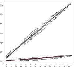
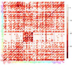
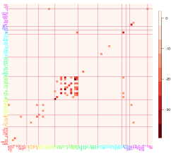
(d) 15/11/2003–07/06/2006	(e) 08/06/2006–17/03/2008	(f) 08/07/2009–28/07/2011

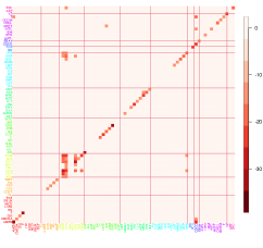
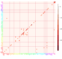
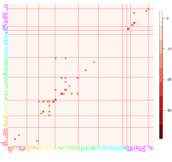
Figure 1: (a) The two largest eigenvalues of the long-run covariance matrix estimated from the volatility panel analysed in Section 5.3 (18/03/2008–07/07/2009, $n=223$) with subsets of cross-sections randomly sampled $100$ times for each given dimension $p\in\{5,\ldots,72\}$ ($x$-axis). (b) and (c): logged and truncated $p$-values from fitting a VAR($5$) model to the same dataset without and with factor-adjustment. (d)–(f): logged and truncated $p$-values similarly obtained with factor-adjustment from the same variables over different periods. In (b)–(f), for each pair of variables, the minimum $p$-value over the five lags is reported. Corresponding tickers are given in $x$- and $y$-axes and industrial sectors are indicated by the colours and boundaries drawn.

VAR modelling quickly becomes a high-dimensional problem as the number of parameters grows quadratically with the dimensionality. Accordingly, most existing methods for detecting change points in high-dimensional, piecewise stationary VAR processes assumes sparsity (Basu and Michailidis,, 2015). However, it is debatable whether highly sparse models are appropriate for some applications. For example, Giannone et al., (2021) note the difficulty of identifying sparse predictive representations for several macroeconomic applications.

We illustrate the inadequacy of the sparsity assumption on a volatility panel dataset (see Section 5.3 for its description). Figure 1 (a) shows that as the dimensionality increases, the leading eigenvalue of the spectral density matrix at frequency $0$ (i.e. the long-run covariance) estimated from the data also increases linearly. This indicates the presence of strong serial and cross-sectional correlations that cannot be accommodated by sparse VAR models. In Figure 1 (b), we report the logged and truncated $p$-values obtained from fitting a VAR($5$) model to the same dataset (truncation level chosen at $\log(3.858\times 10^{-6})$ by Bonferroni correction with the significance level $0.1$) via ridge regression, see Cule et al., (2011). Strong dependence observed from most pairs of the variables further confirms that we cannot infer a sparse pairwise relationship from such data. On the other hand, Figure 1 (c) shows that once we estimate factors driving the strong correlations and adjust for their presence, there is evidence that the remaining dependence in the data can be modelled as being sparse. Together, the plots (d), (e), (c) and (f) display that the relationship between a pair of variables (after factor-adjustment) varies over time, particularly at the level of industrial sectors. Here, the intervals are chosen according to the data segmentation result reported in Section 5.3. This example highlights the importance of (i) accounting for the dominant correlations prior to fitting a model under the sparsity assumption, and (ii) detecting structural changes when analysing time series datasets covering a long period.

Motivated by the aforementioned characteristics of high-dimensional time series data, factor-adjusted regression modelling has increasingly gained popularity (Fan et al.,, 2020, 2021; Krampe and Margaritella,, 2021). The factor-adjusted VAR model proposed by Barigozzi et al., (2022) assumes that a handful of common factors capture strong serial and cross-sectional correlations, such that it is reasonable to assume a sparse VAR model on the remaining component to capture idiosyncratic, variable-specific dependence. We extend this framework by proposing a new, piecewise stationary factor-adjusted VAR model and develop FVARseg, an accompanying change point detection methodology. Below we summarise the methodological and theoretical contributions made in this paper.

Generality of the modelling framework.

We decompose the data into two piecewise stationary latent processes: one is driven by factors and accounts for dominant serial and cross-sectional correlations, and the other models sparse pairwise dependence via a VAR model. We adopt the most general approach to factor modelling and allow both components to undergo changes which, in the case of the latter, are attributed to shifts in the VAR parameters. To the best of our knowledge, such a general model simultaneously permitting the presence of common factors and change points, has not been studied in the literature previously. Accordingly, we are not aware of any method that can comprehensively address the data segmentation problem considered in this paper.

Methodological novelty.

The idea of scanning the data for changes over moving windows, has successfully been applied to a variety of data segmentation problems (Preuss et al.,, 2015; Eichinger and Kirch,, 2018; Chen et al.,, 2021). We propose FVARseg, a two-stage methodology that combines this idea with statistics carefully designed to have good detection power against different types of changes in the two latent components. In Stage 1 of FVARseg, motivated by that dominant factor-driven correlations appear as leading eigenvalues in the frequency domain, see e.g. Figure 1 (a), we propose a detector statistic that contrasts the local spectral density matrix estimators from neighbouring moving windows in operator norm, which is well-suited to detect changes in the factor-driven component.

In Stage 2 for detecting change points in the latent piecewise stationary VAR process, we deliberately avoid estimating the latent process which may incur large errors. Instead, we make use of (i) the Yule-Walker equation that relates autocovariances (ACV) and VAR parameters, and (ii) the availability of local ACV estimators of the latent VAR process after Stage 1. Combining these ingredients, we propose a novel detector statistic that enjoys methodological simplicity as well as statistical efficiency. Further, through sequential evaluation of the detector statistic, the second-stage procedure requires the estimation of local VAR parameters at selected locations only. Consequently it is highly competitive computationally when both the sample size and the dimensionality are large.

Theoretical consistency.

FVARseg achieves consistency in estimating the total number and locations of the change points in both of the piecewise stationary factor-driven and VAR processes. Our theoretical analysis is conducted in a setting considerably more general than those commonly adopted in the literature, permitting dependence across stationary segments and heavy-tailedness of the data. We also derive the rate of localisation for each stage of FVARseg where we make explicit the influence of tail behaviour and the size of changes. In particular, under Gaussianity, the estimators from Stage 1 nearly matches the minimax optimal rate derived for the simpler, covariance change point detection problem.

The rest of the paper is structured as follows. Section 2 introduces the piecewise stationary factor-adjusted VAR model. Section 3 describes the two stages of FVARseg, the proposed data segmentation methodology, and Section 4 establishes its theoretical consistency. Section 5 demonstrates the good performance of FVARseg empirically. R code implementing our method is available from https://github.com/haeran-cho/fvarseg.

Notation.

Let $\mathbf{I}$ and $\mathbf{O}$ denote an identity matrix and a matrix of zeros whose dimensions depend on the context. For a random variable $X$ and $\nu\geq 1$, denote $\|X\|_{\nu}=(\mathsf{E}|X|^{\nu})^{1/\nu}$. Given $\mathbf{A}=[a_{ii^{\prime}},\,1\leq i\leq m,\,1\leq i^{\prime}\leq n]$, we denote by $\mathbf{A}^{*}$ its transposed complex conjugate. We define its element-wise $\ell_{\infty}$, $\ell_{1}$ and $\ell_{2}$-norms by $|\mathbf{A}|_{\infty}=\max_{i,i^{\prime}}|a_{ii^{\prime}}|$, $|\mathbf{A}|_{1}=\sum_{i,i^{\prime}}|a_{ii^{\prime}}|$ and $|\mathbf{A}|_{2}=\sqrt{\sum_{i,i^{\prime}}|a_{ii^{\prime}}|^{2}}$, and its spectral and induced $L_{1}$, $L_{\infty}$-norms by $\|\mathbf{A}\|$, $\|\mathbf{A}\|_{1}=\max_{1\leq i^{\prime}\leq n}\sum_{i=1}^{m}|a_{ii^{\prime}}|$ and $\|\mathbf{A}\|_{\infty}=\max_{1\leq i\leq n}\sum_{i^{\prime}=1}^{m}|a_{ii^{\prime}}|$, respectively. For positive definite $\mathbf{A}$, we denote its minimum eigenvalue by $\|\mathbf{A}\|_{\min}$. For two real numbers, $a\vee b=\max(a,b)$ and $a\wedge b=\min(a,b)$. For two sequences $\{a_{n}\}$ and $\{b_{n}\}$, we write $a_{n}\asymp b_{n}$ if, for some constants $C_{1},C_{2}>0$, there exists $N\in\mathbb{N}$ such that $C_{1}\leq a_{n}b_{n}^{-1}\leq C_{2}$ for all $n\geq N$.

2 Piecewise stationary factor-adjusted VAR model

2.1 Background

A zero-mean, $p$-variate process $\bm{\xi}_{t}$ follows a VAR($d$) model if it satisfies

$$\bm{\xi}_{t}=\mathbf{A}_{1}\bm{\xi}_{t-1}+\ldots+\mathbf{A}_{d}\bm{\xi}_{t-d}+(\bm{\Gamma})^{1/2}\bm{\varepsilon}_{t},$$ (1)

where $\mathbf{A}_{\ell}\in\mathbb{R}^{p\times p},\,1\leq\ell\leq d$, determine how future values of the series depend on their past. The $p$-variate random vector $\bm{\varepsilon}_{t}=(\varepsilon_{1t},\ldots,\varepsilon_{pt})^{\top}$ has $\varepsilon_{it}$ which are independently and identically distributed (i.i.d.) for all $i$ and $t$ with $\mathsf{E}(\varepsilon_{it})=0$ and $\mathsf{Var}(\varepsilon_{it})=1$. The positive definite matrix $\bm{\Gamma}\in\mathbb{R}^{p\times p}$ is the covariance matrix of the innovations for the VAR process.

A factor-driven component exhibits strong cross-sectional and/or serial correlations by ‘loading’ finite-dimensional factors linearly. Among many, the generalised dynamic factor model (GDFM, Forni et al.,, 2000, 2015) provides the most general approach (see Appendix D for further discussions), and defines the $p$-variate factor-driven component $\bm{\chi}_{t}$ as

$$\bm{\chi}_{t}=\mathcal{B}(L)\mathbf{u}_{t}=\sum_{\ell=0}^{\infty}\mathbf{B}_{\ell}\mathbf{u}_{t-\ell}.$$ (2)

For fixed $q$, the $q$-variate random vector $\mathbf{u}_{t}=(u_{1t},\ldots,u_{qt})^{\top}$ contains the common factors which are shared across the variables and time, and $u_{jt}$ are assumed to be i.i.d. for all $j$ and $t$ with $\mathsf{E}(u_{jt})=0$ and $\mathsf{Var}(u_{jt})=1$. The matrix of square-summable filters $\mathcal{B}(L)=\sum_{\ell=0}^{\infty}\mathbf{B}_{\ell}L^{\ell}$ with the lag-operator $L$ and $\mathbf{B}_{\ell}\in\mathbb{R}^{p\times q}$, serves the role of loadings under (2).

Barigozzi et al., (2022) propose a factor-adjusted VAR model, where the observations are assumed to be decomposed as a sum of the two latent components $\bm{\xi}_{t}$ and $\bm{\chi}_{t}$ in (1)–(2), with pervasive correlations in the data are accounted for by $\bm{\chi}_{t}$ and the remaining dependence captured by $\bm{\xi}_{t}$. In the next section, we introduce its piecewise stationary extension where both the factor-driven and VAR processes are allowed to undergo structural changes.

2.2 Model

We observe a zero-mean, $p$-variate piecewise stationary process $\mathbf{X}_{t}=\bm{\chi}_{t}+\bm{\xi}_{t}$ where

$$\left\{\begin{array}[]{ll}\bm{\chi}_{t}=\bm{\chi}_{t}^{[k]}=\mathcal{B}^{[k]}(L)\mathbf{u}_{t}&\text{for \ }\theta_{\chi,k}+1\leq t\leq\theta_{\chi,k+1},\,0\leq k\leq K_{\chi},\\ \bm{\xi}_{t}=\bm{\xi}_{t}^{[k]}=\sum_{\ell=1}^{d}\mathbf{A}^{[k]}_{\ell}\bm{\xi}_{t-\ell}+(\bm{\Gamma}^{[k]})^{1/2}\bm{\varepsilon}_{t}&\text{for \ }\theta_{\xi,k}+1\leq t\leq\theta_{\xi,k+1},\,0\leq k\leq K_{\xi}.\end{array}\right.$$ (5)

Here, $\theta_{\chi,k},\,1\leq k\leq K_{\chi}$, denote the change points in the piecewise stationary factor-driven component $\bm{\chi}_{t}$ such that at each $\theta_{\chi,k}$, the filter of loadings $\mathcal{B}^{[k]}(L)$ undergoes a change. We permit the factor number to vary over time as $q_{k}\leq q$, with the factor $\mathbf{u}^{[k]}_{t}\in\mathbb{R}^{q_{k}}$ associated with $\bm{\chi}^{[k]}_{t}$ being a sub-vector of $\mathbf{u}_{t}\in\mathbb{R}^{q}$. Similarly, $\theta_{\xi,k},\,1\leq k\leq K_{\xi}$, denote the change points in the piecewise stationary VAR process $\bm{\xi}_{t}$ at which the VAR parameters undergo shifts; we permit the VAR innovation covariance matrix to vary as $\bm{\Gamma}^{[k]}$ but our interest lies in detecting changes in VAR parameters, and the VAR order may vary over time as $d_{k}\leq d$ with $\mathbf{A}^{[k]}_{\ell}=\mathbf{O}$ for $\ell\geq d_{k}+1$. By convention, we denote $\theta_{\chi,0}=\theta_{\xi,0}=0$ and $\theta_{\chi,K_{\chi}+1}=\theta_{\xi,K_{\xi}+1}=n$. In line with the factor modelling literature, we assume that $\bm{\chi}_{t}$ and $\bm{\xi}_{t}$ are uncorrelated through having $\mathsf{E}(u_{jt}\varepsilon_{it^{\prime}})~{}=~{}0$ for any $i,j,t$ and $t^{\prime}$.

The model (5) does not require that the change points in $\bm{\chi}_{t}$ and $\bm{\xi}_{t}$ are aligned, or that $K_{\chi}=K_{\xi}$. Our goal is to estimate the total number and locations of the change points for both of the piecewise stationary latent processes. Importantly, we allow $\{\bm{\xi}^{[k]}_{t},\,t\in\mathbb{Z}\}$ (resp. $\{\bm{\chi}^{[k]}_{t},\,t\in\mathbb{Z}\}$) to be dependent across $k$ through sharing the innovations $\bm{\varepsilon}_{t}$ (resp. $\mathbf{u}_{t}$). This makes our model considerably more general than those found in the literature on (high-dimensional) data segmentation under VAR models (Wang et al.,, 2019; Safikhani and Shojaie,, 2022; Bai et al.,, 2022) which assume independence across the segments. Data segmentation under factor models has been considered by Barigozzi et al., (2018) and Li et al., (2022) but they adopt a static approach to factor modelling.

2.3 Assumptions

We introduce assumptions that ensure the (asymptotic) identifiability of the two latent processes in (5) which are framed in terms of spectral properties, as well as controlling the degree of dependence in the data. Denote by $\bm{\Gamma}^{[k]}_{\chi}(\ell)=\mathsf{E}(\bm{\chi}^{[k]}_{t-\ell}(\bm{\chi}^{[k]}_{t})^{\top})$ the ACV matrix of $\bm{\chi}^{[k]}_{t}$ at lag $\ell\in\mathbb{Z}$, and its spectral density matrix at frequency $\omega\in[-\pi,\pi]$ by $\bm{\Sigma}^{[k]}_{\chi}(\omega)=(2\pi)^{-1}\sum_{\ell=-\infty}^{\infty}\bm{\Gamma}^{[k]}_{\chi}(\ell)e^{-\iota\ell\omega}$ with $\iota=\sqrt{-1}$. Then, $\mu^{[k]}_{\chi,j}(\omega),\,1\leq j\leq q_{k}$, denote the real, positive eigenvalues of $\bm{\Sigma}^{[k]}_{\chi}(\omega)$ ordered by decreasing size. We similarly define $\bm{\Gamma}^{[k]}_{\xi}(\ell)$, $\bm{\Sigma}^{[k]}_{\xi}(\omega)$ and $\mu^{[k]}_{\xi,j}(\omega)$ for $\bm{\xi}^{[k]}_{t}$.

Assumption 2.1.

For each $0\leq k\leq K_{\chi}$, the following holds: There exist a positive integer $p_{0}\geq 1$, pairs of functions $\omega\mapsto\alpha^{[k]}_{j}(\omega)$ and $\omega\mapsto\beta^{[k]}_{j}(\omega)$ for $\omega\in[-\pi,\pi]$ and $1\leq j\leq q_{k}$, and $r_{k,j}\in(0,1]$ satisfying $r_{k,1}\geq\ldots\geq r_{k,q_{k}}$ such that for all $p\geq p_{0}$,

$$\beta^{[k]}_{1}(\omega)\geq\frac{\mu^{[k]}_{\chi,1}(\omega)}{p^{r_{k,1}}}\geq\alpha^{[k]}_{1}(\omega)>\ldots>\beta^{[k]}_{q_{k}}(\omega)\geq\frac{\mu^{[k]}_{q_{k}}(\omega)}{p^{r_{k,q_{k}}}}\geq\alpha^{[k]}_{q_{k}}(\omega)>0.$$

If $r_{k,j}=1$ for all $1\leq j\leq q_{k}$ as frequently assumed in the literature (Fan et al.,, 2013; Forni et al.,, 2015), we are in the presence of $q_{k}$ factors which are equally pervasive for the whole cross-sections of $\bm{\chi}^{[k]}_{t}$. If $r_{k,j}<1$ for some $j$, we permit the presence of ‘weak’ factors. Since our primary interest lies in change point analysis, we later introduce a related but distinct condition on the size of change in $\bm{\chi}_{t}$ in Assumption 4.2.

Assumption 2.2.

1. $\det(\sum_{\ell=1}^{d}\mathbf{A}^{[k]}_{\ell}z^{\ell})\neq 0$ for all $|z|\leq 1$ and $0\leq k\leq K_{\xi}$.

2. $m_{\varepsilon}\leq\min_{0\leq k\leq K_{\xi}}\|\bm{\Gamma}^{[k]}\|_{\min}\leq\max_{0\leq k\leq K_{\xi}}\|\bm{\Gamma}^{[k]}\|\leq M_{\varepsilon}$ for some constants $0<m_{\varepsilon}\leq M_{\varepsilon}$.

3. Consider the Wold decomposition $\bm{\xi}^{[k]}_{t}=\sum_{\ell=0}^{\infty}\mathbf{D}^{[k]}_{\ell}(\bm{\Gamma}^{[k]})^{1/2}\bm{\varepsilon}_{t-\ell}$ where $\mathbf{D}^{[k]}_{\ell}=[D^{[k]}_{\ell,ij},\,1\leq i,j\leq p]$. Then, there exist constants $\Xi>0$ and $\varsigma>2$ such that we have $C_{ij},\,1\leq i,j\leq p$, satisfying $\max\{\max_{1\leq j\leq p}\sum_{i=1}^{p}C_{ij},\max_{1\leq i\leq p}\sum_{j=1}^{p}C_{ij},\max_{1\leq i\leq p}\sqrt{\sum_{j=1}^{p}C_{ij}^{2}}\}\leq\Xi$ with which $\max_{0\leq k\leq K_{\xi}}|D^{[k]}_{\ell,ij}|\leq C_{ij}(1+\ell)^{-\varsigma}$ for all $\ell\geq 0$.

4. $\min_{0\leq k\leq K_{\xi}}\inf_{\omega\in[-\pi,\pi]}\mu^{[k]}_{\xi,p}(\omega)\geq m_{\xi}$ for some fixed constant $m_{\xi}>0$.

Assumption 2.3.

There exist constants $\Xi>0$ and $\varsigma>2$ such that for all $\ell\geq 0$,

$\displaystyle{\max_{0\leq k\leq K_{\chi}}\max_{1\leq i\leq p}|\mathbf{B}^{[k]}_{\ell,i\cdot}|_{2}\leq\Xi(1+\ell)^{-\varsigma}\text{ \ and \ }\max_{0\leq k\leq K_{\chi}}\sqrt{\sum_{j=1}^{q_{k}}|\mathbf{B}^{[k]}_{\ell,\cdot j}|_{\infty}^{2}}\leq\Xi(1+\ell)^{-\varsigma}.}$

Assumption 2.2 (i)–(ii) are standard conditions in the literature (Lütkepohl,, 2005; Basu and Michailidis,, 2015). Under condition (iii) and Assumption 2.3, we have time-varying serial dependence in $\mathbf{X}_{t}$ (across all segments) decay at an algebraic rate according to the functional dependence measure of Zhang and Wu, (2021), which is required for controlling the error in locally estimating spectral density and ACV matrices of $\mathbf{X}_{t}$. Assumption 2.2 (iii) allows for mild cross-correlations in $\bm{\xi}^{[k]}_{t}$ while ensuring that $\mu^{[k]}_{\xi,1}(\omega)$ is uniformly bounded:

Proposition 2.1.

Under Assumption 2.2, uniformly over all $\omega\in[-\pi,\pi]$, there exists some $M_{\xi}>0$ depending only on $M_{\varepsilon}$, $\Xi$ and $\varsigma$ such that $\max_{0\leq k\leq K_{\xi}}\sup_{\omega\in[-\pi,\pi]}\mu^{[k]}_{\xi,1}(\omega)\leq M_{\xi}$.

Remark 2.1.

Proposition 2.1, together with Assumption 2.2 (iv), establishes the boundedness of the eigenvalues of $\bm{\Sigma}^{[k]}_{\xi}(\omega)$, which is commonly assumed in the high-dimensional VAR literature for the consistency of Lasso estimators. Assumption 2.2 (iv) holds if there exists some constant $\Xi<\infty$ satisfying $\max(\max_{1\leq j\leq p}\sum_{\ell=1}^{d}|\mathbf{A}^{[k]}_{\ell,\cdot j}|_{1},\max_{1\leq i\leq p}\sum_{\ell=1}^{d}|\mathbf{A}^{[k]}_{\ell,i\cdot}|_{1})\leq\Xi$ (Basu and Michailidis,, 2015). When $d=1$, we have $\mathbf{D}^{[k]}_{\ell}=(\mathbf{A}^{[k]}_{1})^{\ell}$ such that if $|\mathbf{A}^{[k]}_{1}|_{\infty}\leq\gamma<1$, Assumption 2.2 (iii) is readily satisfied with $\max(\|\mathbf{D}^{[k]}_{\ell}\|_{1},\|\mathbf{D}^{[k]}_{\ell}\|_{\infty})\leq\Xi\gamma^{\ell-1}$.

From Assumption 2.1 and Proposition 2.1, the latent components in (5) are asymptotically identifiable as $p\to\infty$, thanks to the gap between $\mu^{[k]}_{\chi,q_{k}}(\omega)$ diverging with $p$ and $\mu^{[k]}_{\xi,1}(\omega)$ which is uniformly bounded, which agrees with the phenomenon observed in Figure 1 (a).

3 Methodology

3.1 Stage 1: Factor-driven component segmentation

3.1.1 Change point detection

The spectral density matrix of $\bm{\chi}_{t}$ is given by $\bm{\Sigma}^{[k]}_{\chi}(\omega)=(2\pi)^{-1}\mathcal{B}^{[k]}(e^{-\iota\omega})(\mathcal{B}^{[k]}(e^{-\iota\omega}))^{*}$ for $\theta_{\chi,k}+1\leq t\leq\chi_{\chi,k+1}$, i.e. it varies over time in a piecewise constant manner with change points at $\theta_{\chi,k},\,1\leq k\leq K_{\chi}$. By Weyl’s inequality, Assumption 2.1 and Proposition 2.1 jointly indicate a gap in the eigenvalues of (time-varying) spectral density matrix of $\mathbf{X}_{t}$, i.e. those attributed to the factor-driven component diverges with $p$ while the remaining ones are bounded for all $p$. This suggests an approach that looks for changes in $\bm{\chi}_{t}$ from the behaviour of $\mathbf{X}_{t}$ in the frequency domain which we further justify below.

Example 3.1.

Suppose that $\bm{\chi}_{t}$ contains a single change point at $t=\theta_{\chi,1}$ at which a new factor is introduced, i.e. $\bm{\chi}^{[0]}_{t}=\mathcal{B}^{[0]}(L)\mathbf{u}_{t}^{[0]}$ and $\bm{\chi}^{[1]}_{t}=\mathcal{B}^{[1]}(L)\mathbf{u}_{t}^{[1]}=\mathcal{B}^{[0]}(L)\mathbf{u}_{t}^{[0]}+\mathbf{b}(L)v_{t}$ with $\mathbf{u}^{[1]}_{t}=((\mathbf{u}_{t}^{[0]})^{\top},v_{t})^{\top}$, which leads to $\bm{\Sigma}^{[1]}_{\chi}(\omega)-\bm{\Sigma}^{[0]}_{\chi}(\omega)=\mathbf{b}(e^{-\iota\omega})\mathbf{b}^{*}(e^{-\iota\omega})/(2\pi)$. Then, from the uncorrelatedness between $\bm{\chi}_{t}$ and $\bm{\xi}_{t}$ and Proposition 2.1, the time-varying spectral density of $\mathbf{X}_{t}$, $\bm{\Sigma}_{x,t}(\omega)$, satisfies $\|\sum_{t=1}^{\theta_{\chi,1}}\bm{\Sigma}_{x,t}(\omega)/\theta_{\chi,1}-\sum_{t=\theta_{\chi,1}+1}^{n}\bm{\Sigma}_{x,t}(\omega)/(n-\theta_{\chi,1})\|=\|\mathbf{b}(e^{-\iota\omega})\mathbf{b}^{*}(e^{-\iota\omega})\|/(2\pi)+O(1)$. That is, the change in the spectral density of $\bm{\chi}_{t}$ is detectable as a change in time-varying spectral density matrix of $\mathbf{X}_{t}$ in operator norm, with the size of change diverging with $p$ as $\|(\mathbf{b}(e^{-\iota\omega}))^{*}\mathbf{b}(e^{-\iota\omega})\|$ does so under Assumption 2.1.

Thus, we detect changes in $\bm{\chi}_{t}$ by scanning for any large change in the spectral density matrix of $\mathbf{X}_{t}$ measured in operator norm, and propose the following moving window-based approach. Given a bandwidth $G$, we estimate the local spectral density matrix of $\mathbf{X}_{t}$ by

$$\widehat{\bm{\Sigma}}_{x,v}(\omega,G) =\frac{1}{2\pi}\sum_{\ell=-m}^{m}K\left(\frac{\ell}{m}\right)\widehat{\bm{\Gamma}}_{x,v}(\ell,G)\exp(-\iota\ell\omega)\quad\text{for}\quad G\leq v\leq n,$$ (6)

where $K(\cdot)$ denotes the Bartlett kernel, $m=G^{\beta}$ the kernel bandwidth with $\beta\in(0,1)$, and

$$\widehat{\bm{\Gamma}}_{x,v}(\ell,G)=\frac{1}{G}\sum_{t=v-G+1+\ell}^{v}\mathbf{X}_{t-\ell}\mathbf{X}_{t}^{\top}\text{ for }\ell\geq 0,\text{ \ and \ }\widehat{\bm{\Gamma}}_{x,v}(\ell,G)=\widehat{\bm{\Gamma}}_{x,v}^{\top}(-\ell,G)\text{ for }\ell<0.$$ (7)

Then the following statistic

$$T_{\chi,v}(\omega,G)=\left\|\widehat{\bm{\Sigma}}_{x,v}(\omega,G)-\widehat{\bm{\Sigma}}_{x,v+G}(\omega,G)\right\|,\quad G\leq v\leq n-G,$$ (8)

serves as a good proxy of the difference in local spectral density matrices of $\bm{\chi}_{t}$ over $I_{v}(G)=\{v-G+1,\ldots,v\}$ and $I_{v+G}(G)=\{v+1,\ldots,v+G\}$. To make it more precise, let $\bm{\Sigma}_{\chi,v}(\omega,G)$ denote a weighted average $\sum_{k=0}^{K_{\chi}}w_{\chi,k}(v)\bm{\Sigma}^{[k]}_{\chi}(\omega)$ with weights $w_{\chi,k}(v)$ corresponding to the proportion of $\bm{\chi}_{t},\,t\in I_{v}(G)$, belonging to $\bm{\chi}^{[k]}_{t}$ (see (F.1)). Then, $T^{*}_{\chi,v}(\omega,G)=\|\bm{\Sigma}_{\chi,v}(\omega,G)-\bm{\Sigma}_{\chi,v+G}(\omega,G)\|$, as a function of $v$, linearly increases and then decreases around the change points with a peak of size $\|\bm{\Sigma}^{[k]}_{\chi}(\omega)-\bm{\Sigma}^{[k+1]}_{\chi}(\omega)\|$ formed at $v=\theta_{\chi,k}$ for all $1\leq k\leq K_{\chi}$, provided that the bandwidth $G$ is not too large (in the sense of Assumption 4.2 (ii) below). The detector statistic $T_{\chi,v}(\omega,G)$ is designed to approximate $T^{*}_{\chi,v}(\omega,G)$ when $\bm{\chi}_{t}$ is not directly observed, and thus is well-suited to detect and locate the change points therein. Unlike other methods for detecting changes in the factor structure (e.g. Li et al.,, 2022), we do not require the number of factors, either for each segment or for the whole dataset, as an input for the construction of $T_{\chi,v}(\omega,G)$.

Once $T_{\chi,v}(\omega_{l},G)$ is evaluated at the Fourier frequencies $\omega_{l}=2\pi l/(2m+1),\,0\leq l\leq m$, we adapt the maximum-check of Eichinger and Kirch, (2018) for simultaneous detection of the multiple change points. Taking the pointwise maximum over the frequencies at each given location $v$, we check if $T_{\chi,v}(\omega(v),G)$ exceeds some threshold $\kappa_{n,p}$ where $\omega(v)$ denotes the frequency at which $T_{v}(\omega_{l},G)$ is maximised, i.e. $\omega(v)=\arg\max_{\omega_{l}:\,0\leq l\leq m}T_{v}(\omega_{l},G)$. If so, it provides evidence that a change point $\theta_{\chi,k}$ is located near the time point $v$, but some care is needed to avoid detecting duplicate estimators, since the detector statistic is expected to take a large value over an interval containing $\theta_{\chi,k}$. Therefore, denoting by $\mathcal{I}\subset\{G,\ldots,n-G\}$ the set containing all time points at which $T_{\chi,v}(\omega(v),G)>\kappa_{n,p}$, we regard $\widehat{\theta}=\arg\max_{v\in\mathcal{I}}T_{\chi,v}(\omega(v),G)$ as a change point estimator if it is a local maximiser of $T_{\chi,v}(\omega(\widehat{\theta}),G)$ within an interval of radius $\eta G$ centred at $\widehat{\theta}$ with some $\eta\in(0,1)$, i.e. $T_{\chi,\widehat{\theta}}(\omega(\widehat{\theta}),G)\geq\max_{\widehat{\theta}-\eta G<v\leq\widehat{\theta}+\eta G}T_{\chi,v}(\omega(\widehat{\theta}),G)$. Once $\widehat{\theta}$ is added to the set of final estimators, say $\widehat{\Theta}_{\chi}$, in order to avoid the risk of duplicate estimators, we remove the interval of radius $G$ centred at $\widehat{\theta}$ from $\mathcal{I}$, and repeat the same procedure with the maximiser of $T_{\chi,v}(\omega(v),G)$ at time points $v$ remaining in $\mathcal{I}$ until the set $\mathcal{I}$ is empty. Algorithm 1 in Appendix C outlines the steps of Stage 1 of FVARseg.

3.1.2 Post-segmentation factor adjustment

Following the detection of change points in $\bm{\chi}_{t}$, we are able to estimate the segment-specific quantities related to $\bm{\chi}^{[k]}_{t}$. In view of the second-stage of FVARseg detecting change points in $\bm{\xi}_{t}$, we describe how to estimate $\bm{\Gamma}^{[k]}_{\chi}(\ell)$ with which we can estimate the ACV of $\bm{\xi}_{t}$.

For each $k=0,\ldots,\widehat{K}_{\chi}$, we first estimate the spectral density of $\mathbf{X}_{t}$ over the segment $\{\widehat{\theta}_{\chi,k}+1,\ldots,\widehat{\theta}_{\chi,k+1}\}$ by $\widehat{\bm{\Sigma}}_{x}^{[k]}(\omega)$ as in (6) using the sample ACV computed from the segment (we use the same kernel bandwidth $m$ for simplicity). Then noting that the spectral density matrix of $\bm{\chi}^{[k]}_{t}$ is of rank $q_{k}$ under (5), we estimate it from the eigendecomposition of $\widehat{\bm{\Sigma}}^{[k]}_{x}(\omega_{l})$ by retaining only the $q_{k}$ largest eigenvalues, say $\widehat{\mu}^{[k]}_{x,j}(\omega_{l})$, and the associated eigenvectors $\widehat{\mathbf{e}}^{[k]}_{x,j}(\omega_{l})$, and then estimate the ACV of $\bm{\chi}^{[k]}_{t}$ by inverse Fourier transform, i.e.

$$\widehat{\bm{\Sigma}}_{\chi}^{[k]}(\omega_{l})=\sum_{j=1}^{q_{k}}\widehat{\mu}^{[k]}_{x,j}(\omega_{l})\widehat{\mathbf{e}}^{[k]}_{x,j}(\omega_{l})\left(\widehat{\mathbf{e}}^{[k]}_{x,j}(\omega_{l})\right)^{*}\text{ and }\widehat{\bm{\Gamma}}_{\chi}^{[k]}(\ell)=\frac{2\pi}{2m+1}\sum_{l=-m}^{m}\widehat{\bm{\Sigma}}^{[k]}_{\chi}(\omega_{l})e^{\iota\omega_{l}\ell}.$$ (9)

The estimators in (9) require the factor number $q_{k}$ as an input. We refer to Hallin and Liška, (2007) for an information criterion (IC)-based estimator of $q_{k}$ that make use of the postulated eigengap in the spectral density matrix of $\mathbf{X}_{t}$.

3.2 Stage 2: Piecewise VAR process segmentation

Applying the existing VAR segmentation methods in our setting requires estimating the $np$ elements of the latent piecewise stationary VAR process $\bm{\xi}_{t}$, which introduces additional errors and possibly results in the loss of statistical efficiency. In addition, as discussed in Appendix A.2, the existing methods tend to be computationally demanding, e.g. by evaluating the Lasso estimators $O(n^{2})$ times in a dynamic programming algorithm, or solving a large fused Lasso objective function of dimension $np^{2}d$. Instead, since we can estimate the local AVC of $\bm{\xi}_{t}$ from the post-segmentation factor-adjustment in Stage 1, our proposed methodology for segmenting the latent VAR component avoids estimating $\bm{\xi}_{t}$ directly. Also, as described below, the proposed method evaluates the local VAR parameters at carefully selected locations only, and thus is computationally efficient.

Specifically, our approach makes use of the Yule-Walker equation (Lütkepohl,, 2005). Let $\bm{\beta}^{[k]}=[\mathbf{A}^{[k]}_{1},\ldots,\mathbf{A}^{[k]}_{d}]^{\top}\in\mathbb{R}^{(pd)\times p}$ contain all VAR parameters in the $k$th segment. Then, it is related to the ACV matrices $\bm{\Gamma}^{[k]}_{\xi}(\ell)=\mathsf{E}(\bm{\xi}^{[k]}_{t-\ell}(\bm{\xi}^{[k]}_{t})^{\top})$ as $\mathbbm{G}^{[k]}\bm{\beta}^{[k]}=\mathbbm{g}^{[k]}$, where

$$\mathbbm{G}^{[k]}=\begin{bmatrix}\bm{\Gamma}^{[k]}_{\xi}(0)&\bm{\Gamma}^{[k]}_{\xi}(-1)&\ldots&\bm{\Gamma}^{[k]}_{\xi}(-d+1)\\ &&\ddots&\\ \bm{\Gamma}^{[k]}_{\xi}(d-1)&\bm{\Gamma}^{[k]}_{\xi}(d-2)&\ldots&\bm{\Gamma}^{[k]}_{\xi}(0)\end{bmatrix}\quad\text{and}\quad\mathbbm{g}^{[k]}=\begin{bmatrix}\bm{\Gamma}^{[k]}_{\xi}(1)\\ \vdots\\ \bm{\Gamma}^{[k]}_{\xi}(d)\end{bmatrix},$$ (10)

with $\mathbbm{G}^{[k]}$ being invertible due to Assumption 2.2 (iv). We propose to utilise this estimating equation in combination with the local ACV estimators of $\bm{\xi}_{t}$ obtained as described below.

For a given bandwidth $G$ and the interval $I_{v}(G)=\{v-G+1,\ldots,v\}$, we estimate the ACV of $\bm{\xi}_{t}$ for $t\in I_{v}(G)$, by $\widehat{\bm{\Gamma}}_{\xi,v}(\ell,G)=\widehat{\bm{\Gamma}}_{x,v}(\ell,G)-\widehat{\bm{\Gamma}}_{\chi,v}(\ell,G)$. Here, $\widehat{\bm{\Gamma}}_{x,v}(\ell,G)$ is defined in (7) and $\widehat{\bm{\Gamma}}_{\chi,v}(\ell,G)$ is a weighted average of $\widehat{\bm{\Gamma}}^{[k]}_{\chi}(\ell),\,0\leq k\leq\widehat{K}_{\chi}$, the estimators of ACV of $\bm{\chi}^{[k]}_{t}$ in (9), with the weights given by the proportion of $I_{v}(G)$ covered by the $k$th segment (see (F.16) for the precise definition). Replacing $\bm{\Gamma}^{[k]}_{\xi}(\ell)$ with $\widehat{\bm{\Gamma}}_{\xi,v}(\ell,G)$, we obtain $\widehat{\mathbbm{G}}_{v}(G)$ estimating a weighted average of $\mathbbm{G}^{[k]}$, and similarly $\widehat{\mathbbm{g}}_{v}(G)$. Then, we propose to scan $T_{\xi,v}(\widehat{\bm{\beta}},G)={|\kern-1.07639pt|\kern-1.07639pt|(\widehat{\mathbbm{G}}_{v}(G)\widehat{\bm{\beta}}-\widehat{\mathbbm{g}}_{v}(G))-(\widehat{\mathbbm{G}}_{v+G}(G)\widehat{\bm{\beta}}-\widehat{\mathbbm{g}}_{v+G}(G))|\kern-1.07639pt|\kern-1.07639pt|}$ with some inspection parameter $\widehat{\bm{\beta}}\in\mathbb{R}^{(pd)\times p}$ and a matrix norm ${|\kern-1.07639pt|\kern-1.07639pt|\cdot|\kern-1.07639pt|\kern-1.07639pt|}$. We motivate this statistic by considering $T^{*}_{\xi,v}(\widehat{\bm{\beta}},G)={|\kern-1.07639pt|\kern-1.07639pt|(\mathbbm{G}_{v}(G)\widehat{\bm{\beta}}-\mathbbm{g}_{v}(G))-(\mathbbm{G}_{v+G}(G)\widehat{\bm{\beta}}-\mathbbm{g}_{v+G}(G))|\kern-1.07639pt|\kern-1.07639pt|}$, its population counterpart. With appropriately chosen $G$ (see Assumption 4.4 (ii) below), $T^{*}_{\xi,v}(\widehat{\bm{\beta}},G)=0$ if $v$ is far from all the change points in $\bm{\xi}_{t}$, i.e. $\min_{k}|v-\theta_{\xi,k}|\geq G$, while it is tent-shaped near the change points with a local maximum at $v=\theta_{\xi,k}$, provided that

$$\mathbbm{G}^{[k-1]}(\widehat{\bm{\beta}}-\bm{\beta}^{[k-1]})\neq\mathbbm{G}^{[k]}(\widehat{\bm{\beta}}-\bm{\beta}^{[k]}).$$ (11)

For the inspection parameter, we adopt an $\ell_{1}$-regularised Yule-Walker estimator of the VAR parameters first considered by Barigozzi et al., (2022) in stationary settings. At given $v_{\circ}\in\{G,\ldots,n\}$, we solve the constrained $\ell_{1}$-minimisation problem

$$\widehat{\bm{\beta}}_{v_{\circ}}(G)={\arg\min}_{\bm{\beta}\in\mathbb{R}^{pd\times p}}|\bm{\beta}|_{1}\quad\text{subject to}\quad\left|\widehat{\mathbbm{G}}_{v_{\circ}}(G)\bm{\beta}-\widehat{\mathbbm{g}}_{v_{\circ}}(G)\right|_{\infty}\leq\lambda_{n,p},$$ (12)

with a tuning parameter $\lambda_{n,p}>0$. The $\ell_{\infty}$-constraint in (12) naturally leads to the choice ${|\kern-1.07639pt|\kern-1.07639pt|\cdot|\kern-1.07639pt|\kern-1.07639pt|}=|\cdot|_{\infty}$, resulting in the following detector statistic:

$$T_{\xi,v}(\widehat{\bm{\beta}},G)=\left|\left(\widehat{\mathbbm{G}}_{v}(G)\widehat{\bm{\beta}}-\widehat{\mathbbm{g}}_{v}(G)\right)-\left(\widehat{\mathbbm{G}}_{v+G}(G)\widehat{\bm{\beta}}-\widehat{\mathbbm{g}}_{v+G}(G)\right)\right|_{\infty}.$$

For good detection power, the condition in (11) suggests using an estimator of $\bm{\beta}^{[k-1]}$ or $\bm{\beta}^{[k]}$ in place of $\widehat{\bm{\beta}}$ for detecting $\theta_{\xi,k}$. Therefore, we propose to evaluate $T_{\xi,v}(\widehat{\bm{\beta}}_{v_{\circ}}(G),G)$ for $v\geq G$, with $\widehat{\bm{\beta}}_{v_{\circ}}(G)$ updated sequentially at locations strategically selected as below.

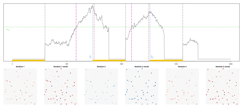
Figure 2: Illustration of Stage 2 applied to a realisation from (M1) of Section 5.2 with $G=300$ and $d=1$. Top: The solid curve represents $T_{\xi,v}(\widehat{\bm{\beta}},G),\,v_{\circ}\leq v\leq\check{\theta}+G$, computed at the three iterations of Steps 1–3 of Algorithm 2. At each iteration, we use $\widehat{\bm{\beta}}=\widehat{\bm{\beta}}_{v_{\circ}}(G)$ estimated from each of the subsections the data highlighted in the $x$-axis (left to right); the corresponding estimators are plotted in the bottom panel and for comparison, we also plot the estimators obtained in the oracle setting where $\bm{\xi}_{t}$ is observable (all plots have the identical $z$-axis range). The locations of $v_{\circ}$, $\check{\theta}$ and $\widehat{\theta}$ in Algorithm 2, and $\theta_{\xi,k}$ are denoted by the vertical long-dashed, dot-dashed, dotted and dashed lines, respectively. The horizontal line represents $\pi_{n,p}$ chosen as described in Section 5.1.

First we estimate $\bm{\beta}^{[0]}$ by $\widehat{\bm{\beta}}=\widehat{\bm{\beta}}_{G}(G)$ in (12) with $v_{\circ}=G$ and scan the data using $T_{\xi,v}(\widehat{\bm{\beta}},G),\,v\geq v_{\circ}$. When $T_{\xi,v}(\widehat{\bm{\beta}},G)$ exceeds some threshold, say $\pi_{n,p}$, at $v=\check{\theta}$ for the first time, it signifies that a change has occurred in the neighbourhood. Reducing the search for a change point to $\{\check{\theta},\ldots,\check{\theta}+G\}$, we identify a change point estimator as the local maximiser $\widehat{\theta}_{\xi,1}=\arg\max_{\check{\theta}\leq v\leq\check{\theta}+G}T_{\xi,v}(\widehat{\bm{\beta}},G)$. Then updating $\widehat{\bm{\beta}}$ with $\widehat{\bm{\beta}}_{v_{\circ}}(G)$ obtained at $v_{\circ}=\widehat{\theta}_{\xi,1}+(\eta+1)G$ for some $\eta\in(0,1]$ (i.e. only using an interval of length $G$ located strictly to the right of $\widehat{\theta}_{\xi,1}$ for its computation), we continue screening $T_{\xi,v}(\widehat{\bm{\beta}},G),\,v\geq v_{\circ}$, until it next exceeds $\pi_{n,p}$. These steps of screening $T_{\xi,v}(\widehat{\bm{\beta}},G)$ and updating $\widehat{\bm{\beta}}$ are repeated iteratively until the end of the data sequence is reached. Algorithm 2 in Appendix C outlines the steps of the Stage 2 methodology.

Figure 2 illustrates that although $\bm{\xi}_{t}$ is latent, at each iteration, $\widehat{\bm{\beta}}_{v_{\circ}}(G)$ does as well as its oracle counterpart (obtained as in (12) with the sample ACV of $\bm{\xi}_{t}$ replacing $\widehat{\bm{\Gamma}}_{\xi,v}(\ell,G)$). Computationally, this strategy benefits from that the costly solution to the $\ell_{1}$-minimisation problem in (12) is required (at most) $K_{\xi}+1$ times with an appropriately chosen threshold $\pi_{n,p}$ (see Theorem 4.3 below). We further demonstrate numerically the competitiveness of Stage 2 as a standalone method for VAR time series segmentation in Section 5.2, and provide an in-depth comparative study with the existing methods in Appendix A.2.

4 Theoretical properties

4.1 Consistency of Stage 1 of FVARseg

We carry out our theoretical investigation under two different regimes with respect to the tail behaviour of $\mathbf{u}_{t}$ and $\bm{\xi}_{t}$; in particular, the weaker condition in Assumption 4.1 (i) permits heavy-tailed innovations, while the existing literature on (piecewise stationary) VAR modelling in high dimensions, commonly adopts the Gaussianity as in (ii).

Assumption 4.1.

We assume either of the following conditions.

1. There exists $\nu>4$ such that $\max\left\{\mathsf{E}(|u_{jt}|^{\nu}),\mathsf{E}(|\varepsilon_{it}|^{\nu})\right\}\leq\mu_{\nu}<\infty$.

2. $\mathbf{u}_{t}\sim_{\mbox{\scriptsize{iid}}}\mathcal{N}_{q}(\mathbf{0},\mathbf{I})$ and $\bm{\varepsilon}_{t}\sim_{\mbox{\scriptsize{iid}}}\mathcal{N}_{p}(\mathbf{0},\mathbf{I})$.

In establishing the consistency of Stage 1, we opt to measure the size of changes in $\bm{\chi}_{t}$ using ${\bm{\Delta}}_{\chi,k}(\omega)=\bm{\Sigma}_{\chi}^{[k]}(\omega)-\bm{\Sigma}_{\chi}^{[k-1]}(\omega)$, $1\leq k\leq K_{\chi}$, the difference in spectral density matrices of $\bm{\chi}_{t}$ from neighbouring segments. As ${\bm{\Delta}}_{\chi,k}(\omega)$ is Hermitian, we can always find the $j$th largest (in modulus), real-valued eigenvalue of ${\bm{\Delta}}_{\chi,k}(\omega)$ which we denote by $\mu_{j}({\bm{\Delta}}_{\chi,k}(\omega))$, with $\mu_{1}({\bm{\Delta}}_{\chi,k}(\omega))=\|{\bm{\Delta}}_{\chi,k}(\omega)\|$. Recall that $m=G^{\beta}$ for some $\beta\in(0,1)$, denotes the bandwidth used in local spectral density estimation, see (6).

Assumption 4.2.

1. For each $1\leq k\leq K_{\chi}$, the following holds: There exist a positive integer $p_{0}\geq 1$ and pairs of functions $\omega\mapsto a^{[k]}_{j}(\omega)$ and $\omega\mapsto b^{[k]}_{j}(\omega)$ for $\omega\in[-\pi,\pi]$ and $j=1,2$, and $r^{\prime}_{k,1}\in(0,1]$ and $r^{\prime}_{k,2}\in[0,1]$ satisfying $r^{\prime}_{k,1}\geq r^{\prime}_{k,2}$, such that

   $$b^{[k]}_{1}(\omega)\geq\frac{\mu_{1}({\bm{\Delta}}_{\chi,k}(\omega))}{p^{r^{\prime}_{k,1}}}\geq a^{[k]}_{1}(\omega)>b^{[k]}_{2}(\omega)\geq\frac{\mu_{2}({\bm{\Delta}}_{\chi,k}(\omega))}{p^{r^{\prime}_{k,2}}}\geq a^{[k]}_{2}(\omega)\geq 0$$

   for all $p\geq p_{0}$. Besides, we assume that the functions $\omega\mapsto p^{-r^{\prime}_{k,1}}\mu_{1}({\bm{\Delta}}_{\chi,k}(\omega))$ are Lipschitz continuous with bounded Lipschitz constants. Then for $\Delta_{\chi,k}=\max_{\omega\in[-\pi,\pi]}\mu_{1}({\bm{\Delta}}_{\chi,k}(\omega))$, we have $\max_{1\leq k\leq K_{\chi}}\Delta_{\chi,k}^{-1}\cdot p(\psi_{n}\vee m^{-1})=o(1)$, where

   $$\psi_{n}=\left\{\begin{array}[]{ll}\frac{n^{2/\nu}m\log^{2+2/\nu}(G)}{G}\vee\sqrt{\frac{m\log(n)}{G}}&\text{under Assumption~{}\ref{assum:innov}~{}\ref{cond:moment}},\\ \sqrt{\frac{m\log(n)}{G}}&\text{under Assumption~{}\ref{assum:innov}~{}\ref{cond:gauss}.}\end{array}\right.$$ (15)

2. The bandwidth $G=G_{n}$ satisfies $G_{n}\to\infty$ as $n\to\infty$ while fulfilling

   $$\min\left\{\min_{0\leq k\leq K_{\chi}}(\theta_{\chi,k+1}-\theta_{\chi,k}),\min_{0\leq k\leq K_{\xi}}(\theta_{\xi,k+1}-\theta_{\xi,k})\right\}\geq 2G.$$ (16)

Assumption 4.2 specifies the detection lower bound which is determined by $\min_{k}\Delta_{\chi,k}$ and $\min_{k}(\theta_{\chi,k+1}-\theta_{\chi,k})$ (through $G$), for all $K_{\chi}$ change points $\bm{\chi}_{t}$ to be detectable by Stage 1. Condition (i) requires $\mu_{1}({\bm{\Delta}}_{\chi,k}(\omega))$ to be distinct from the rest. In fact, the remaining $\mu_{j}(\bm{\Delta}_{\chi,k}(\omega)),\,j\geq 2$, are allowed to be exactly zero, which is the case in Example 3.1; here, we have $\Delta_{\chi,1}=\max_{\omega}(2\pi)^{-1}\|(\mathbf{b}(e^{-\iota\omega}))^{*}\mathbf{b}(e^{-\iota\omega})\|$ where $\mathbf{b}(z)$ is a $p$-variate vector of factor loading filters. The rate $p(\psi_{n}\vee m^{-1})$ represents the bias-variance trade-off when estimating the local spectral density matrix of $\bm{\chi}_{t}$ by $\widehat{\bm{\Sigma}}_{x,v}(G,\omega)$ (see Proposition F.6). It is possible to find the rate of kernel bandwidth $m$ that minimises this rate depending on the tail behaviour of $X_{it}$ (e.g. $m\asymp(G/\log(n))^{1/3}$ under Gaussianity), but we choose to explicitly highlight the role of this tuning parameter on our results.

Theorem 4.1.

Suppose that Assumptions 2.1–2.3, 4.1 and 4.2 hold. Let $\kappa_{n,p}$ satisfy

$$2Mp\left(\psi_{n}\vee\frac{1}{m}\vee\frac{1}{p}\right)<\kappa_{n,p}<\frac{1}{2}\min_{1\leq k\leq K_{\chi}}\Delta_{\chi,k}-Mp\left(\psi_{n}\vee\frac{1}{m}\vee\frac{1}{p}\right)$$

for some constant $M>0$. Then, there exists a set $\mathcal{M}^{\chi}_{n,p}$ with $\mathsf{P}(\mathcal{M}^{\chi}_{n,p})\to 1$ as $n,p\to\infty$, such that the following holds for $\widehat{\Theta}_{\chi}=\{\widehat{\theta}_{\chi,k},\,1\leq k\leq\widehat{K}_{\chi}:\,\widehat{\theta}_{\chi,1}<\ldots<\widehat{\theta}_{\chi,\widehat{K}_{\chi}}\}$ returned by Stage 1 of FVARseg, on $\mathcal{M}^{\chi}_{n,p}$ for large enough $n$ and $p$:

1. $\widehat{K}_{\chi}=K_{\chi}$ and $\max_{1\leq k\leq K_{\chi}}|\widehat{\theta}_{\chi,k}-\theta_{\chi,k}|\leq\epsilon_{0}G$ for some $\epsilon_{0}\in(0,1/2)$ with $\eta\in(2\epsilon_{0},1]$.

2. There exists a constant $c_{0}>0$ such that for all $1\leq k\leq K_{\chi}$, $|\widehat{\theta}_{\chi,k}-\theta_{\chi,k}|\leq c_{0}\rho^{[k]}_{n,p}$ where

   $$\rho^{[k]}_{n,p}=\left(\frac{\Delta_{\chi,k}}{p}\right)^{-2}\times\left\{\begin{array}[]{ll}m^{\frac{\nu}{\nu-2}}(GK_{\chi})^{\frac{2}{\nu-2}}&\text{under Assumption~{}\ref{assum:innov}~{}\ref{cond:moment}},\\ m\log(GK_{\chi})&\text{under Assumption~{}\ref{assum:innov}~{}\ref{cond:gauss}}.\end{array}\right.$$

Remark 4.1.

1. In Theorem 4.1 (b), $\rho^{[k]}_{n,p}$ reflects the difficulty associated with estimating the individual change point $\theta_{\chi,k}$ manifested by $(p^{-1}\Delta_{\chi,k})^{-2}$. In the Gaussian case (Assumption 4.1 (ii)), the localisation rate $\rho^{[k]}_{n,p}$ is always sharper than $G$ due to Assumption 4.2 (i). Considering the problem of covariance change point detection in independent, sub-Gaussian random vectors in high dimensions, Wang et al., (2021) derive the minimax lower bound on the localisation rate in their Lemma 3.2, and $\rho^{[k]}_{n,p}$ matches this rate up to $m\log(n)$; here, the dependence on the kernel bandwidth $m$ is attributed to that we consider a time series segmentation problem, i.e. a change may occur in the ACV of $\bm{\chi}_{t}$ at lags other than zero. If heavier tails are permitted (Assumption 4.1 (i)), $\rho^{[k]}_{n,p}$ can be tighter than $\epsilon_{0}G$, e.g. when $\Delta_{\chi,k}\asymp p$, $K_{\chi}$ is fixed and $m\asymp G^{\beta}$ for some $\beta\in(0,1-4/\nu)$.

2. Empirically, replacing $\widehat{\theta}$ with $\widetilde{\theta}=\arg\max_{v\in\mathcal{I}}\,\text{avg}_{l}T_{\chi,v}(\omega_{l},G)$ returns a more stable location estimator, where $\text{avg}_{l}$ denotes the average operator over $l=0,\ldots,m$. We can derive the localisation rate for $\widetilde{\theta}$ similarly as in Theorem 4.1 (b) with $\widetilde{\Delta}_{\chi,k}=\pi^{-1}\int_{0}^{\pi}\|{\bm{\Delta}}_{\chi,k}(\omega)\|d\omega$ in place of $\Delta_{\chi,k}$. Our numerical results in Section 5.2 are based on this estimator.

Next, we establish the consistency of $\widehat{\bm{\Gamma}}^{[k]}_{\chi}(\ell)$ in (9) estimating the segment-specific ACV of $\bm{\chi}^{[k]}_{t}$ under the following assumption on the strength of factors.

Assumption 4.3.

Assumption 2.1 holds with $r_{k,j}=1$ for all $1\leq j\leq q_{k}$ and $0\leq k\leq K_{\chi}$.

Theorem 4.2.

Suppose that Assumption 4.3 holds in addition to the assumptions made in Theorem 4.1, and define $\rho_{n,p}=\max_{1\leq k\leq K_{\chi}}\min(\epsilon_{0}G,\rho^{[k]}_{n,p})$. Also let

$$\vartheta_{n,p} =\left\{\begin{array}[]{ll}\frac{m(np)^{2/\nu}\log^{7/2}(p)}{G}\vee\sqrt{\frac{m\log(np)}{G}}&\text{under Assumption~{}\ref{assum:innov}~{}\ref{cond:moment}},\\ \sqrt{\frac{m\log(np)}{G}}&\text{under Assumption~{}\ref{assum:innov}~{}\ref{cond:gauss}}.\end{array}\right.$$ (19)

Then on $\mathcal{M}^{\chi}_{n,p}$ defined in Theorem 4.1, for some finite integer $d\in\mathbb{N}$, we have

$$\max_{0\leq k\leq K_{\chi}}\max_{0\leq\ell\leq d}\left|\widehat{\bm{\Gamma}}^{[k]}_{\chi}(\ell)-\bm{\Gamma}^{[k]}_{\chi}(\ell)\right|_{\infty}=O_{p}\left(\vartheta_{n,p}\vee\frac{1}{m}\vee\frac{\rho_{n,p}}{G}\vee\frac{1}{\sqrt{p}}\right).$$

It is possible to work under the weaker Assumption 2.1 and trace the effect of weak factors or bound estimation errors measured in different norms. Corollary C.16 of Barigozzi et al., (2022) derives such results in the stationary setting, where an additional multiplicative factor of $p^{2(1-\min_{k}r_{k,q_{k}})}$ appears in the $O_{P}$-bound in Theorem (4.2). We work under the stronger Assumption 4.3 as it simplifies the presentation of Theorem 4.2 which plays an important role in the investigation into Stage 2 of FVARseg, and since only Assumption 4.3 is compatible with the cross-sectional ordering often being completely arbitrary.

4.2 Consistency of Stage 2 of FVARseg

Suppose that the tuning parameter for the $\ell_{1}$-regularised Yule-Walker estimation problem in (12), is set with some constant $M>0$ and $\vartheta_{n,p}$ and $\rho_{n,p}$ defined in Theorem 4.2, as

$$\lambda_{n,p} =M\left(\max_{0\leq k\leq K_{\xi}}\|\bm{\beta}^{[k]}\|_{1}+1\right)\left(\vartheta_{n,p}\vee\frac{1}{m}\vee\frac{\rho_{n,p}}{G}\vee\frac{1}{\sqrt{p}}\right).$$ (20)

This choice reflects the error in $\widehat{\bm{\Gamma}}_{\xi,v}(\ell,G)$ estimating the local ACV of $\bm{\xi}_{t}$ over all $v$ and $\ell$.

The following assumption imposes conditions on the size of the changes in VAR parameters and the minimum spacing between the change points.

Assumption 4.4.

1. For each $1\leq k\leq K_{\xi}$, let ${\bm{\Delta}}_{\xi,k}=\mathbbm{G}^{[k]}(\bm{\beta}^{[k]}-\bm{\beta}^{[k-1]})$. Then,

   $$\max_{1\leq k\leq K_{\xi}}\frac{(1\vee\|\mathbbm{G}^{[k]}(\mathbbm{G}^{[k-1]})^{-1}\|_{1})\lambda_{n,p}}{|{\bm{\Delta}}_{\xi,k}|_{\infty}}=o(1).$$

2. The bandwidth $G$ fulfils (16), i.e. $\min_{0\leq k\leq K_{\xi}}(\theta_{\xi,k+1}-\theta_{\xi,k})\geq 2G$.

Remark 4.2.

We choose to measure the size of change using $|\bm{\Delta}_{\xi,k}|_{\infty}$. From Assumption 2.2 (iv), we have ${\bm{\Delta}}_{\xi,k}=\mathbf{O}$ iff $\bm{\beta}^{[k]}-\bm{\beta}^{[k-1]}=\mathbf{O}$. In the related literature, the $\ell_{2}$-norm $|\bm{\beta}^{[k]}-\bm{\beta}^{[k-1]}|_{2}$ scaled by the global sparsity (given by the union of the supports of all $\bm{\beta}^{[k]},\,0\leq k\leq K_{\xi}$), is used to measure the size of change where this global sparsity may be much greater than that of $\bm{\Delta}_{\xi,k}$ when $K_{\xi}$ is large, see Appedix A.2. In some instances, we have $\mathbbm{G}^{[k]}(\mathbbm{G}^{[k-1]})^{-1}=\mathbf{I}$, e.g. when $d=1$ and $\mathbf{A}_{1}^{[k]}=-\mathbf{A}_{1}^{[k-1]}$ such that Assumption 4.4 (i) becomes $\lambda_{n,p}=o(\min_{k}|\bm{\Delta}|_{\infty})$. More generally, bounding $\|\mathbbm{G}^{[k]}(\mathbbm{G}^{[k-1]})^{-1}\|_{1}$ implicitly assumes (approximate) sparsity on the second-order structure of $\bm{\xi}_{t}$. When $d=1$, we have $\mathbbm{G}^{[k]}=\sum_{\ell=0}^{\infty}(\mathbf{A}^{[k]}_{1})^{\ell}\bm{\Gamma}^{[k]}[(\mathbf{A}^{[k]}_{1})^{\top}]^{\ell}$ such that the boundedness of $\|\mathbbm{G}^{[k]}\|_{1}$ and $\|(\mathbbm{G}^{[k]})^{-1}\|_{1}$ follows when $\mathbf{A}^{[k]}_{1}$ and $\bm{\Gamma}^{[k]}$ are block diagonal with fixed block size (Wang and Tsay,, 2022). For general $d\geq 1$, we have $\|\mathbbm{G}^{[k]}(\mathbbm{G}^{[k-1]})^{-1}\|_{1}$ bounded if $\mathbbm{G}^{[k]}$ are strictly diagonally dominant (see Definition 6.1.9 of Horn and Johnson, (1985) and Han et al., (2015)), which is met e.g. when $\mathbf{A}^{[k]}_{\ell}$ are diagonal with their diagonal entries fulfilling $\gamma^{[k]}_{\xi,ii}(0)>2\sum_{\ell=1}^{d-1}|\gamma^{[k]}_{\xi,ii}(\ell)|$ (where $\bm{\Gamma}^{[k]}_{\xi}(\ell)=[\gamma^{[k]}_{\xi,ii^{\prime}}(\ell)]_{i,i^{\prime}}$); this trivially holds when $d=1$.

Theorem 4.3.

Suppose that Assumption 4.4 holds in addition to the assumptions made in Theorem 4.2. With $\lambda_{n,p}$ chosen as in (20), we set $\pi_{n,p}$ to satisfy

$$2\lambda_{n,p}<\pi_{n,p}<\frac{1}{2}\min_{1\leq k\leq K_{\xi}}|{\bm{\Delta}}_{\xi,k}|_{\infty}.$$

Then, there exists a set $\mathcal{M}^{\xi}_{n,p}$ with $\mathsf{P}(\mathcal{M}^{\xi}_{n,p})\to 1$ as $n,p\to\infty$, such that the following holds for $\widehat{\Theta}_{\xi}=\{\widehat{\theta}_{\xi,k},\,1\leq k\leq\widehat{K}_{\xi}:\,\widehat{\theta}_{\xi,1}<\ldots<\widehat{\theta}_{\xi,\widehat{K}_{\xi}}\}$ returned by Stage 2 of FVARseg, on $\mathcal{M}^{\xi}_{n,p}$ for large enough $n$:

1. $\widehat{K}_{\xi}=K_{\xi}$ and $\max_{1\leq k\leq K_{\xi}}|\widehat{\theta}_{\xi,k}-\theta_{\xi,k}|\leq\epsilon_{0}G$ for some $\epsilon_{0}\in(0,1/2)$ with $\eta\in(\epsilon_{0},1]$.

2. There exists a constant $c_{0}>0$ such that for all $1\leq k\leq K_{\xi}$ satisfying $\{\theta_{\xi,k}-2G+1,\ldots,\theta_{\xi,k}+2G\}\cap\Theta_{\chi}=\emptyset$, we have $|\widehat{\theta}_{\xi,k}-\theta_{\xi,k}|\leq c_{0}\varrho^{[k]}_{n,p}$, where

   $$\varrho^{[k]}_{n,p}=|{\bm{\Delta}}_{\xi,k}|_{\infty}^{-2}\left(1+\max_{0\leq k\leq K_{\xi}}\|\bm{\beta}^{[k]}\|_{1}\right)\times\left\{\begin{array}[]{l}(GK_{\xi}p)^{\frac{2}{\nu-2}}\log^{\frac{3\nu}{\nu-2}}(p)\\ \qquad\text{under Assumption~{}\ref{assum:innov}~{}\ref{cond:moment}},\\ \log(GK_{\xi}p)\\ \qquad\text{under Assumption~{}\ref{assum:innov}~{}\ref{cond:gauss}}.\end{array}\right.$$

Due to the sequential nature of FVARseg, the success of Stage 2 is conditional on that of Stage 1 which occurs on an asymptotic one-set, see Theorem 4.1. Theorem 4.3 (a) establishes that Stage 2 of FVARseg consistently detects all $K_{\xi}$ change points within the distance of $\epsilon_{0}G$ where $\epsilon_{0}$ can be made arbitrarily small as $n,p\to\infty$ under Assumption 4.4 (i). Theorem 4.3 (b) shows that a further refined localisation rate can be derived for $\theta_{\xi,k}$ when it is sufficiently distanced away from the change points in the factor-driven component. If, say, $\theta_{\xi,k}$ lies close to $\theta_{\chi,k^{\prime}}$, a change point in $\bm{\chi}_{t}$, the error from estimating the local ACV of $\bm{\xi}_{t}$ due to the bias in $\widehat{\theta}_{\chi,k^{\prime}}$, prevents applying the arguments involved in the refinement to such $\theta_{\xi,k}$. The refined rate $\varrho^{[k]}_{n,p}$ is always tighter than $G$ under Gaussianity.

It is of independent interest to consider the cases where $\bm{\chi}_{t}$ is stationary (i.e. $K_{\chi}=0$) or where we directly observe the piecewise stationary VAR process (i.e. $\mathbf{X}_{t}=\bm{\xi}_{t}$). Consistency of the Stage 2 of FVARseg readily extends to such settings and the improved localisation rates in Theorem 4.3 (b) apply to all the estimators. Also, further improvement is attained in the heavy-tailed situations (Assumption 4.1 (i)) if $\bm{\xi}_{t}$ is directly observable. For the full statement of the results, we refer to Corollary A.1 in Appendix A where we also provide a detailed comparison between Stage 2 of FVARseg and existing VAR segmentation methods (that do not take into the possible presence of factors), both theoretically and numerically.

5 Empirical results

5.1 Numerical considerations

Multiscale extension.

The bandwidth $G$ is required to be large enough to provide a good local estimators of spectral density of $\bm{\chi}_{t}$ (Stage 1) and VAR parameters (Stage 2). However, if $G$ is too large, we may have windows that contain two or more changes when scanning the data for change points, which violates Assumptions 4.2 (ii) and 4.4 (ii). Cho and Kirch, (2022) note the lack of adaptivity of a single-bandwidth moving window procedure in the presence of multiscale change points (a mixture of large changes over short intervals and smaller changes over long intervals), and advocates the use of multiple bandwidths. Accordingly we also propose to apply FVARseg with a range of bandwidths and prune down the outputs using a ‘bottom-up’ method (Messer et al.,, 2014; Meier et al.,, 2021). Let $\widehat{\Theta}(G)$ denote the output from Stage 1 or 2 with a bandwidth $G$. Given a set of bandwidths $\mathcal{G}=\{G_{h},\,1\leq h\leq H:\,G_{1}<\ldots<G_{H}\}$, we accept all estimators from the finest $G_{1}$ to the set of final estimators $\widehat{\Theta}$ and sequentially for $h\geq 2$, accept $\widehat{\theta}\in\widehat{\Theta}(G_{h})$ iff $\min_{\check{\theta}\in\widehat{\Theta}}|\widehat{\theta}-\check{\theta}|\geq G/2$. In simulation studies, we use $\mathcal{G}_{\chi}=\{[n/10],[n/8],[n/6],[n/4]\}$ for Stage 1, and $\mathcal{G}_{\xi}$ generated as an equispaced sequence between $[2.5p]$ and $[n/4]$ of length $4$ for Stage 2. The choice of $\mathcal{G}_{\xi}$ is motivated by the simulation results of Barigozzi et al., (2022) under the stationarity, where the $\ell_{1}$-regularised estimator in (12) was observed to performs well when the sample size exceeds $2p$.

Speeding up Stage 1.

The computational bottleneck of FVARseg is the computation of $T_{\chi,v}(\omega_{l},G)$ in Stage 1, which involves singular value decomposition (SVD) of a $p\times p$-matrix at multiple frequencies and over time. We propose to evaluate $T_{\chi,v}(\omega_{l},G)$ on a grid $v\in\{G+ab_{n}:\,0\leq a\leq\lfloor(n-2G)/b_{n}\rfloor\}$ with $b_{n}=\lfloor 2\log(n)\rfloor$. This may incur additional bias of at most $b_{n}/2\leq\log(n)$ in change point location estimation which is asymptotically negligible in view of Theorem 4.1, but reduce the computational load by the factor of $b_{n}$.

Selection of thresholds.

The theoretically permitted ranges of $\kappa_{n,p}$ and $\pi_{n,p}$ (see Theorems 4.1 and 4.3) depend on constants which are not accessible or difficult to estimate in practice. This is an issue commonly encountered by data segmentation methods which involve localised testing, and often a reasonable solution is found by large-scale simulations, an approach we also take. We use simulations to derive a simple rule for selecting the threshold as a function of $n$, $p$ and $G$. For this, we (i) propose a scaling for each of the two detector statistics adopted in Stages 1 and 2 which reduces its dependence on the data generating process, and (ii) fit a linear model for an appropriate percentile of the scaled detector statistics obtained from simulated datasets. Specifically, we simulate $B=100$ time series following (5) with $K_{\chi}=K_{\xi}=0$ using the models considered in Section 5.2, and record the maximum of the scaled detector statistics $T^{\circ}_{\chi,v}(G)$ and $T^{\circ}_{\xi,v}(G)$ over $v$ on each realisation. Here, the scaling terms are obtained from the first $G$ observations only, as

$$T^{\circ}_{\chi,v}(G)=\max_{0\leq l\leq m}\frac{T_{\chi,v}(\omega_{l},G)}{T_{\chi,G}(\omega_{l},G)}\text{ \ and \ }T^{\circ}_{\xi,v}(G)=\frac{T_{\xi,v}(\widehat{\bm{\beta}}_{G}(G),G)}{\max_{0\leq\ell\leq d}|\widehat{\bm{\Gamma}}_{\xi,[\frac{G}{2}]}(\ell,[\frac{G}{2}])-\widehat{\bm{\Gamma}}_{\xi,G}(\ell,[\frac{G}{2}])|_{\infty}}.$$

Generating the data with varying $(n,p,q,d)$ and repeating the above procedure with multple choices of $G$, we fit a linear model to the $100(1-\tau)$th percentile of $\log(\max_{v}T^{\circ}_{\chi,v}(G))$ with $\log\log(n)$ and $\log(G)$ as regressors ($R^{2}_{\text{adj}}=0.9651$), and use the fitted model to derive a threshold for given $n$ and $G$ that is then applied to the similarly scaled $T^{\circ}_{\chi,v}(\omega_{l},G)$. Analogously, we regress the $100(1-\tau)$th percentile of $\log(\max_{v}T^{\circ}_{\xi,v}(G))$ onto $\log\log(n)$, $\log\log(p)$ and $\log(G)$ ($R^{2}_{\text{adj}}=0.985$), and find a threshold applied to the scaled $T^{\circ}_{\xi,v}(\widehat{\bm{\beta}},G)$ given $n$, $p$ and $G$ from the fitted model. The choice of the regressors is motivated by the definitions of $\psi_{n}$ and $\psi_{n,p}$ which appear in Theorems 4.1 and 4.3. The high values of $R^{2}_{\text{adj}}$ indicate the excellent fit of the linear models and consequently, that the threshold selection rule is insensitive to the data generating processes. When Stage 2 is used as a standalone method for segmenting observed VAR processes, a smaller threshold is recommended which is in line with Corollary A.1, and we find that $\pi_{n,p}=1$ works well with the proposed scaling.

Other tuning parameters.

While data-adaptive methods exist for selecting the kernel window size $m$ in (6) (Politis,, 2003), we find that setting it simply at $m=\max(1,\lfloor G^{1/3}\rfloor)$ for given $G$, works well for the purpose of data segmentation. The results are not highly sensitive to the choice of $\eta$ in Stage 1 and use $\eta=0.5$ throughout. In Stage 2, we find that not trimming off the data when estimating the VAR parameters by setting $\eta=0$, does not hurt the numerical performance. In factor-adjustment, we select the segment-specific factor number $q_{k}$ using the IC-based approach of Hallin and Liška, (2007). Krampe and Margaritella, (2021) propose to jointly select the (static) factor number and the VAR order using an IC but generally, the validity of IC is not well-understood for VAR order selection in high dimensions. In our simulations, following the practice in the literature on VAR segmentation, we regard $d$ as known but also investigate the sensitivity of FVARseg when $d$ is mis-specified. In analysing the panel of daily volatilities (Section 5.3), we use $d=5$ which has the interpretation of the number of trading days per week. Finally, we select $\lambda_{n,p}$ in (12) via cross validation as in Barigozzi et al., (2022).

5.2 Simulation studies

In the simulations, we consider the cases when the factor-driven component is present ($\bm{\chi}_{t}\neq 0$) and when it is not ($\bm{\chi}_{t}=0$). For the former, we consider two models for generating $\bm{\chi}_{t}$ with $q=2$. In the first model, referred to as (C1), $\bm{\chi}_{t}$ admits a static factor model representation while in the second model (C2), it does not; empirically, the task of factor structure estimation is observed to be more challenging under (C2) (Forni et al.,, 2017; Barigozzi et al.,, 2022). We generate $\bm{\xi}_{t}$ as piecewise stationary Gaussian VAR($d$) processes with $d\in\{1,2\}$ and a parameter $\beta$ that controls the size of the change (with smaller $\beta$ indicating the smaller change). We refer to Appendix B.1 for the full descriptions of simulation models and Table 1 for an overview of the $24$ data generating processes which also contains information about the sets of change points $\Theta_{\chi}$ and $\Theta_{\xi}$; under each setting, we generate $100$ realisations. Below we provide a summary of the findings from the simulation studies, and Tables B.1–B.2 reporting the results can be found in Appendix B.2.

Table 1: Data generating processes for simulation studies.

	$n$	$p$	$\bm{\chi}_{t}$	$(d,\beta)$	$\Theta_{\chi}$	$\Theta_{\xi}$
(M1)	$2000$	$50,100,150$	(C1)	$(1,1)$	$\emptyset$, $\{[n/4],[n/2],[3n/4]\}$	$\{[3n/8],[5n/8]\}$
(M2)	$2000$	$50,100,150$	(C2)	$(1,1)$	$\emptyset$, $\{[n/3],[2n/3]\}$	$\{[n/3],[2n/3]\}$
(M3)	$2000$	$50,100,150$	$\mathbf{0}$	$(1,0.6)$, $(2,0.8)$	$\emptyset$	$\emptyset$, $\{[3n/8],[5n/8]\}$

To the best of our knowledge, there does not exist a methodology that comprehensively addresses the change point problem under the model (5). Therefore under (M1)–(M2), we compare the Stage 1 of FVARseg with a method proposed in Barigozzi et al., (2018), referred to as BCF hereafter, on their performance at detecting changes in $\bm{\chi}_{t}$. While BCF has a step for detecting change points in the remainder component, it does so nonparametically unlike the Stage 2 of FVARseg, which may lead to unfair comparison. Hence we separately consider (M3) with $\mathbf{X}_{t}=\bm{\xi}_{t}$ where we compare the Stage 2 method with VARDetect (Safikhani et al.,, 2022), a block-wise variant of Safikhani and Shojaie, (2022).

Results under (M1)–(M2).

Overall, FVARseg achieves good accuracy in estimating the total number and locations of the change points for both $\bm{\chi}_{t}$ and $\bm{\xi}_{t}$ across different data generating processes. Under (M1) adopting the static factor model for generating $\bm{\chi}_{t}$, FVARseg shows similar performance as BCF in detecting $\Theta_{\chi}$ when the dimension is small ($p=50$), but the latter tends to over-estimate the number of change points as $p$ increases. Also, FVARseg outperforms the binary segmentation-based BCF in change point localisation. BCF requires as an input the upper bound on the number of global factors, say $q^{\prime}$, that includes the ones attributed to the change points, and its performance is sensitive to its choice. In (M1), we have $q^{\prime}\leq 3q(K_{\chi}+1)$ (which is supplied to BCF) while in (M2), $\bm{\chi}^{[k]}_{t}$ does not admit a static factor representation and accordingly such $q^{\prime}$ does not exist (we set $q^{\prime}=2q$ for BCF). Accordingly, BCF tends to under-estimate the number of change points under (M2). Generally, the task of detecting change points in $\bm{\xi}_{t}$ is aggravated by the presence of change points in $\bm{\chi}_{t}$ due to the sequential nature of FVARseg, and the Stage 2 performs better when $K_{\chi}=0$ both in terms of detection and localisation accuracy, which agrees with the observations made in Corollary A.1 (a).

Between (M1) and (M2), the latter poses a more challenging setting for the Stage 2 methodology. This may be attributed to (i) the difficulty posed by the data generating scenario (C2), which is observed to make the estimation tasks related to the latent VAR process more difficult (Barigozzi et al.,, 2022), and (ii) that $\Theta_{\chi}=\Theta_{\xi}$ where the estimation bias from Stage 1 has a worse effect on the performance of Stage 2 compared to when $\Theta_{\chi}$ and $\Theta_{\xi}$ do not overlap, see the discussion below Theorem 4.3.

Results under (M3).

Table B.2 shows that the Stage 2 of FVARseg outperforms VARDetect in all criteria considered, particularly as $p$ increases. VARDetect struggles to detect any change point when the change is weak (recall that $\beta=0.6$ is used when $d=1$ which makes the size of change at $\theta_{\xi,2}$ small) or when $d=2$. FVARseg is faster than VARDetect in most situations except for when $(d,p,K_{\xi})=(1,50,0)$, sometimes more than $10$ times e.g. when $d=2$ and there is no change point in the data. Additionally, Stage 2 of FVARseg is insensitive to the over-specification of the VAR order ($d=2$ is used when in fact $d=1$). When it is under-specified, there is slight loss of detection power as expected. Compared to the results obtained under (M1)–(M2), the localisation performance of the Stage 2 method improves in the absence of the factor-driven component, even though the size of changes under (M3) tends to be smaller. This confirms the theoretical findings reported in Corollary A.1 (b) in Appendix A. Although not reported here, when the full FVARseg methodology is applied to the data generated under (M3), the Stage 1 method does not detect any spurious change point estimators as desired.

5.3 Application: US blue chip data

We consider daily stock prices from $p=72$ US blue chip companies across industry sectors between January 3, 2000 and February 16, 2022 ($n=5568$ days), retrieved from the Wharton Research Data Services; the list of companies and their corresponding sectors can be found in Appendix E. Following Diebold and Yılmaz, (2014), we measure the volatility using $\sigma_{it}^{2}=0.361(p_{it}^{\text{high}}-p_{it}^{\text{low}})^{2}$ where $p_{it}^{\text{high}}$ (resp. $p_{it}^{\text{low}}$) denotes the maximum (resp. minimum) log-price of stock $i$ on day $t$, and set $X_{it}=\log(\sigma_{it}^{2})$.

We apply FVARseg to detect change points in the panel of volatility measures $\{X_{it},\,1\leq i\leq p;\,1\leq t\leq n\}$. With $n_{0}=252$ denoting the number of trading days per year, we apply Stage 1 with bandwidths chosen as an equispaced sequence between $[n_{0}/4]$ and $2n_{0}$ of length $4$, implicitly setting the minimum distance between two neighbouring change points to be three months. Based on the empirical sample size requirement for VAR parameter estimation (see Section 5.1), we apply Stage 2 with bandwidths chosen as an equispaced sequence between $2.5p$ and $2n_{0}$ of length $4$. The VAR order is set at $d=5$ which corresponds to the number of trading days in each week, and the rest of the tuning parameters are selected as in Section 5.1. Table 2 reports the segmentation results.

Table 2: Sets of change point estimators returned by FVARseg.

$\widehat{\Theta}_{\chi}$ returned by Stage 1				$\widehat{\Theta}_{\xi}$ returned by Stage 2
2002-06-06	2007-12-10	2008-09-12	2008-12-16	2002-02-04	2003-03-18	2003-11-25	2006-06-07	2008-03-17	2009-07-07
2009-05-11	2020-02-18	2020-05-20		2011-07-28	2013-05-30	2015-06-25	2017-10-03	2020-02-27

Stage 1 detects four change points around the Great Financial Crisis between 2007 and 2009, and the last two estimators from Stage 1 correspond to the onset (2020-02-20) and the end (2020-04-07) of the stock market crash brought in by the instability due to the COVID-19 pandemic. Given the clustering of change points between 2007 and 2009, an alternative approach is to adopt a locally stationary factor model as in Barigozzi et al., (2021). However, such a model does not allow for the number of factors to vary over time, whereas we observe the contrary to be the case when applying the IC-based method of Hallin and Liška, (2007) to each segment defined by $\widehat{\Theta}_{\chi}$, see Table 3. This supports that it is more appropriate to model the changes in the factor-driven component of this dataset as abrupt changes rather than as smooth transitions.

Table 3: Estimated number of factors $\widehat{q}_{k}$ from $\{\mathbf{X}_{t},\,\widehat{\theta}_{\chi,k}+1\leq t\leq\widehat{\theta}_{\chi,k+1}\}$, $k=0,\ldots,7$.

Segment $k$	0	1	2	3	4	5	6	7
$\widehat{q}_{k}$	3	4	2	7	2	5	1	2

The estimators from Stage 2 are spread across the period in consideration. Figure 1 (c)–(f) illustrate how the linkages between different companies vary over the four segments identified between $2003$ and $2011$ particularly at the level of industrial sectors, although this information is not used by FVARseg.

Table 4: Mean and standard errors of $\text{FE}^{\text{avg}}_{t}$ and $\text{FE}^{\text{max}}_{t}$ for $t\in\mathcal{T}$ where $|\mathcal{T}|=1600$.

		$\text{FE}^{\text{avg}}$		$\text{FE}^{\text{max}}$
	Forecasting method	Mean	SE	Mean	SE
(F1)	Restricted	0.7671	0.3729	0.9181	0.1898
	Unrestricted	0.7746	0.4123	0.9204	0.2007
(F2)	Restricted	0.7831	0.4011	0.9217	0.1962
	Unrestricted	0.8138	0.4666	0.9279	0.2008

To further validate the segmentation obtained by FVARseg, we perform a forecasting exercise. Two approaches, referred to as (F1) and (F2) below, are adopted to build forecasting models where the difference lies in how a sub-sample of $\{\mathbf{X}_{u},\,u\leq t-1\}$, is chosen to forecast $\mathbf{X}_{t}$. Simply put, (F1) uses the observations belonging to the same segment as $\mathbf{X}_{t}$ only, for constructing the forecast of $\bm{\chi}_{t}$ (resp. $\bm{\xi}_{t}$) according to the segmentation defined by $\widehat{\Theta}_{\chi}$ (resp. $\widehat{\Theta}_{\xi}$), while (F2) ignores the presence of the most recent change point estimator. We expect (F1) to give more accurate predictions if the data undergoes structural changes at the detected change points. On the other hand, if some of the change point estimators are spurious, (F2) is expected to produce better forecasts since it makes use of more observations. We select $\mathcal{T}$, the set of time points at which to perform forecasting, such that each $t\in\mathcal{T}$ does not belong to the first two segments (i.e. $t\geq\max(\widehat{\theta}_{\chi,2},\widehat{\theta}_{\xi,2})+1$), and there are at least $n_{0}$ of observations to build a forecast model separately for $\bm{\chi}_{t}$ and $\bm{\xi}_{t}$, respectively. Denoting by $\widehat{L}_{\chi}(v)=\max\{0\leq k\leq\widehat{K}_{\chi}:\,\widehat{\theta}_{\chi,k}+1\leq v\}$ the index of $\widehat{\theta}_{\chi,k}$ nearest to and strictly left of $v$ and similarly defining $\widehat{L}_{\xi}(v)$, this means that $\min(\widehat{L}_{\chi}(t),\widehat{L}_{\xi}(t))\geq 2$ and $\min(t-\widehat{\theta}_{\chi,\widehat{L}_{\chi}(t)},t-\widehat{\theta}_{\xi,\widehat{L}_{\xi}(t)})\geq n_{0}$ for all $t\in\mathcal{T}$. We have $|\mathcal{T}|=1600$. For such $t\in\mathcal{T}$, we obtain $\widehat{\mathbf{X}}_{t}(\mathbf{N})=\widehat{\bm{\chi}}_{t}(N_{1})+\widehat{\bm{\xi}}_{t}(N_{2})$ for some $\mathbf{N}=(N_{1},N_{2})$, where $\widehat{\bm{\chi}}_{t}(N_{1})$ denotes an estimator of the best linear predictor of $\bm{\chi}_{t}$ given $\mathbf{X}_{t-\ell},\,1\leq\ell\leq N_{1}$, and $\widehat{\bm{\xi}}_{t}(N_{2})$ is defined analogously. The difference between the two approaches we take lies in the selection of $\mathbf{N}$.

1. We set $N_{1}=t-\widehat{K}_{\chi,\widehat{L}_{\chi}(t)}-1$ and $N_{2}=t-\widehat{K}_{\xi,\widehat{L}_{\xi}(t)}-1$.

2. We set $N_{1}=t-\widehat{K}_{\chi,\widehat{L}_{\chi}(t)-1}-1$ and $N_{2}=t-\widehat{K}_{\xi,\widehat{L}_{\xi}(t)-1}-1$.

Barigozzi et al., (2022) propose two methods for estimating the best linear predictors of $\bm{\chi}_{t}$ and $\bm{\xi}_{t}$ under a stationary factor-adjusted VAR model, one based on a more restrictive assumption on the factor structure (‘restricted’) than the other (‘unrestricted’); we refer to the paper for their detailed descriptions. Both estimators are combined with the two approaches (F1) and (F2). Table 4 reports the summary of the forecasting errors measured as $\text{FE}^{\text{avg}}_{t}=|\mathbf{X}_{t}-\widehat{\mathbf{X}}_{t}(\mathbf{N})|_{2}^{2}/|\mathbf{X}_{t}|_{2}^{2}$ and $\text{FE}^{\text{max}}_{t}=|\mathbf{X}_{t}-\widehat{\mathbf{X}}_{t}(\mathbf{N})|_{\infty}/|\mathbf{X}_{t}|_{\infty}$, obtained from combining different best linear predictors with (F1)–(F2). According to all evaluation criteria, (F1) produces forecasts that are more accurate than (F2) regardless of the forecasting methods, which supports the validity of the change point estimators returned by FVARseg.

Appendix A Further discussions on Stage 2 of FVARseg

A.1 Extension of Theorem 4.3

We consider the performance of the Stage 2 of FVARseg when applied to some special cases under the model (5) where (a) $\bm{\chi}_{t}$ is stationary (i.e. $\Theta_{\chi}=\emptyset$) and (b) we directly observe $\mathbf{X}_{t}=\bm{\xi}_{t}$ (i.e. $\bm{\chi}_{t}=\mathbf{0}$). Theorem 4.1 indicates that in both cases, the Stage 1 of FVARseg returns $\widehat{\Theta}_{\chi}=\emptyset$. The results reported in Theorem 4.3 readily extend to such settings.

Corollary A.1.

Suppose that the assumptions of Theorem 4.3 hold, including Assumption 4.4 (i) with $\lambda_{n,p}$ specified below. Then, with $\varrho^{[k]}_{n,p}$ defined as in Theorem 4.3, i.e.

$$\varrho^{[k]}_{n,p}=|{\bm{\Delta}}_{\xi,k}|_{\infty}^{-2}\left(1+\max_{0\leq k\leq K_{\xi}}\|\bm{\beta}^{[k]}\|_{1}\right)\times\left\{\begin{array}[]{l}(GK_{\xi}p)^{\frac{2}{\nu-2}}\log^{\frac{3\nu}{\nu-2}}(p)\\ \qquad\text{under Assumption~{}\ref{assum:innov}~{}\ref{cond:moment}},\\ \log(GK_{\xi}p)\\ \qquad\text{under Assumption~{}\ref{assum:innov}~{}\ref{cond:gauss}},\end{array}\right.$$

there exist a set $\mathcal{M}^{\xi}_{n,p}$ with $\mathsf{P}(\mathcal{M}^{\xi}_{n,p})\to 1$ as $n,p\to\infty$ and constants $\epsilon_{0},c_{0}>0$ such that on $\mathcal{M}^{\xi}_{n,p}$, we have

$$\widehat{K}_{\xi}=K_{\xi}\quad\text{and}\quad\left|\widehat{\theta}_{\xi,k}-\theta_{\xi,k}\right|\leq\min\left(\epsilon_{0}G,\,c_{0}\varrho^{[k]}_{n,p}\right)\text{ for all }1\leq k\leq K_{\xi}$$

for $n$ large enough, in the following situations.

1. There is no change point in the factor-driven component, i.e. $K_{\chi}=0$, and we set

   $$\lambda_{n,p}=M\left(\max_{0\leq k\leq K_{\xi}}\|\bm{\beta}^{[k]}\|_{1}+1\right)\left(\vartheta_{n,p}\vee\frac{1}{m}\vee\frac{1}{\sqrt{p}}\right).$$

2. We directly observe the piecewise stationary VAR process, i.e. $\mathbf{X}_{t}=\bm{\xi}_{t}$ for all $t$, and we set $\lambda_{n,p}=M(\max_{0\leq k\leq K_{\xi}}\|\bm{\beta}^{[k]}\|_{1}+1)\bar{\vartheta}_{n,p}$ with

   $$\bar{\vartheta}_{n,p}=\left\{\begin{array}[]{ll}\frac{(np)^{2/\nu}\log^{3}(p)\log^{2+2/\nu}(G)}{G}\vee\sqrt{\frac{\log(np)}{G}}&\text{under Assumption~{}\ref{assum:innov}~{}\ref{cond:moment}},\\ \sqrt{\frac{\log(np)}{G}}&\text{under Assumption~{}\ref{assum:innov}~{}\ref{cond:gauss}.}\end{array}\right.$$ (A.3)

When compared to the methods dedicated to the setting corresponding to Corollary A.1 (b), our Stage 2 methodology achieves comparative theoretical performance in terms of the detection lower bound imposed on the size of changes for their detection, and the rate of localisation achieved. We provide a comprehensive comparison of the Stage 2 methodology with the existing VAR segmentation methods in the next section, both on their theoretical and computational properties.

A.2 Comparison with the existing VAR segmentation methods

There are a few methods proposed for time series segmentation under piecewise stationary, Gaussian VAR models, a setting that corresponds to Corollary A.1 (b) under Gaussianity. In this setting, we compare the Stage 2 of FVARseg with those proposed by Wang et al., (2019) and Safikhani and Shojaie, (2022).

Table A.1: Comparison of change point methods developed under piecewise stationary VAR models on their theoretical performance (under Gaussianity) and computational complexity. Here, $\mathfrak{g}=\max_{1\leq k\leq K_{\xi}}\|\mathbbm{G}^{[k]}(\mathbbm{G}^{[k-1]})^{-1}\|_{1}$, $s_{\circ}=|\mathcal{S}|$ denotes the global sparsity defined with $\mathcal{S}\in\{1,\ldots,pd\}\times\{1,\ldots,p\}$ where $[\bm{\beta}^{[k]}]_{i,i^{\prime}}=0$ iff $(i,i^{\prime})\notin\mathcal{S}$ for all $k$. LP($a$) denotes the complexity of solving a linear program with $a$ variables and Lasso($a$, $b$) that of solving a Lasso problem with sample size $a$ and dimensionality $b$.

Methods	Separation	Localisation	Complexity
Stage 2 of FVARseg	$(1\vee\mathfrak{g})^{2}\log(n\vee p)$	$\log(n\vee p)$	$O(G^{-1}np\;\text{LP}(pd)+np^{2})$
Wang et al., (2019)	$s_{\circ}K_{\xi}\log(n\vee p)$	$\log(n\vee p)$	$O(n^{2}p\;\text{Lasso}(n,pd))$
Safikhani and Shojaie, (2022)	$s_{\circ}^{4}K_{\xi}^{2}\log(p)$	$s_{\circ}^{4}K_{\xi}\log(p)$	Not available

Table A.1 summarises the comparative study in terms of their theoretical and computational properties. Denoting by $\bar{\Delta}_{k}$ the size of change between the $(k-1)$th and the $k$th segments (measured differently for different methods), the separation rate refers to some $\nu_{n,p}\to\infty$ such that if $\nu_{n,p}^{-1}\;\min_{k}\bar{\Delta}_{k}^{2}\cdot\min_{k}(\theta_{\xi,k+1}-\theta_{\xi,k})\to\infty$, the corresponding method correctly detects all $K_{\xi}$ change points; for Stage 2, we set $\bar{\Delta}_{k}=|{\bm{\Delta}}_{\xi,k}|_{\infty}$ and for the others, $\bar{\Delta}_{k}=s_{\circ}^{-1/2}|\bm{\beta}^{[k]}-\bm{\beta}^{[k-1]}|_{2}$ (see the caption of Table A.1 for the definition of $s_{\circ}$). The localisation rate refers to some $\varrho_{n,p}\to\infty$ satisfying $\max_{1\leq k\leq K_{\xi}}w_{k}^{2}|\bar{\theta}_{k}-\theta_{\xi,k}|=O_{P}(\varrho_{n,p})$ for the estimators $\bar{\theta}_{k}$ returned by respective methods. For FVARseg, the weights $w_{k}$ reflect the difficulty associated with locating individual change points, i.e. $w_{k}=\bar{\Delta}_{k}$, while for Wang et al., (2019) and Safikhani and Shojaie, (2022), the weights are global with $w_{k}=\min_{k}\bar{\Delta}_{k}$ and $w_{k}=1$, respectively. Safikhani and Shojaie, (2022) further assume that $\min_{k}|\bm{\beta}^{[k]}-\bm{\beta}^{[k-1]}|_{2}$ is bounded away from zero. We suppose that $\max_{k}\|\bm{\beta}^{[k]}\|_{1}=O(1)$, a sufficient condition for the boundedness of $\|\bm{\Sigma}^{[k]}_{\xi}(\omega)\|$ for each segment-specific VAR process (Basu and Michailidis,, 2015, Proposition 2.2), which is required by all the methods in consideration for their theoretical consistency.

Immediate comparison of the theoretical results is difficult due to different definitions of $\bar{\Delta}_{k}$: Observe that

$$|{\bm{\Delta}}_{\xi,k}|_{0}\cdot|{\bm{\Delta}}_{\xi,k}|_{\infty}^{2}\geq|{\bm{\Delta}}_{\xi,k}|_{2}^{2}\geq(2\pi m_{\xi})^{2}|\bm{\beta}^{[k]}-\bm{\beta}^{[k-1]}|_{2}^{2}$$

from Assumption 2.2 (iv), where $|\cdot|_{0}$ denotes the element-wise $\ell_{0}$-norm. Noting that $|\bm{\Delta}_{\xi,k}|_{0}=|\bm{\beta}^{[k]}-\bm{\beta}^{[k-1]}|_{0}$, the requirement of Stage 2 of FVARseg may be stronger than that made in Wang et al., (2019) if $s_{\circ}\asymp|\bm{\beta}^{[k]}-\bm{\beta}^{[k-1]}|_{0}$. On the other hand, we can have $s_{\circ}$ much greater than $|\bm{\beta}^{[k]}-\bm{\beta}^{[k-1]}|_{0}$ if $K_{\xi}$ is large or when the sparsity pattern of $\bm{\beta}^{[k]}$ varies greatly from one segment to another. The method proposed by Safikhani and Shojaie, (2022) is generally worse than the other two both in terms of separation and localisation rates.

The $\ell_{1}$-regularised Yule-Walker estimation problem in (12) can be solved in parallel and further, it needs to be performed only $K_{\xi}+1$ times with large probability, which makes the Stage 2 methodology more attractive. By comparison, the dynamic programming methodology of Wang et al., (2019) requires the Lasso estimation to be performed $O(n^{2})$ times, and the multi-stage procedure of Safikhani and Shojaie, (2022) solves a fused Lasso problem of dimension $np^{2}d$ to obtain pre-estimators of the change points, and then exhaustively searches for the final set of estimators which can be NP-hard in the worst case. In Section 5.2, we compare the Stage 2 methodology with a blockwise modification of Safikhani and Shojaie, (2022) that is implemented in the R package VARDetect (Bai et al.,, 2021).

Finally, we note that there are methods developed under piecewise stationary extensions of the low-rank plus sparse VAR($1$) model proposed in Basu et al., (2019), see Bai et al., (2022). While they additionally permit a low rank structure in the parameter matrices, the spectrum of $\mathbf{X}_{t}$ is assumed to be uniformly bounded which rules out pervasive (serial) correlations in the data and thus is distinguished from the piecewise stationary factor-adjusted VAR model considered in this paper.

Appendix B Further information on simulation studies

B.1 Data generating processes

We provide full details on how the data is generated for numerical experiments reported in Section 5.2. Firstly, the factor-driven component $\bm{\chi}_{t}$ is generated according to the following two models.

1. $\bm{\chi}^{[k]}_{t}$ admits a static factor model representation, as

   $$\chi^{[k]}_{it}=\sum_{j=1}^{q}(B^{[k]}_{0,ij}+B^{[k]}_{1,ij}L+B^{[k]}_{2,ij}L^{2})u_{jt},\quad 0\leq k\leq K_{\chi},$$

   where $u_{jt}\sim_{\mbox{\scriptsize{iid}}}\mathcal{N}(0,\sigma_{j}^{2})$ with $(\sigma_{1},\sigma_{2})=(1,0.5)$, and the MA coefficients are generated as $(B^{[k]}_{0,ij},B^{[k]}_{1,ij},B^{[k]}_{2,ij})\sim_{\mbox{\scriptsize{iid}}}\mathcal{N}_{3}(\mathbf{0},\mathbf{I})$ for all $1\leq i\leq p$ and $1\leq j\leq q$ when $k=0$. Then sequentially for $k=1,\ldots,K_{\chi}$, we draw $\Pi^{[k]}_{\chi}\subset\{1,\ldots,p\}$ with $|\Pi^{[k]}_{\chi}|=[0.5p]$ such that for all $j$, $(B^{[k]}_{0,ij},B^{[k]}_{1,ij},B^{[k]}_{2,ij})\sim_{\mbox{\scriptsize{iid}}}\mathcal{N}_{3}(\mathbf{0},\mathbf{I})$ when $i\in\Pi^{[k]}_{\chi}$ while $(B^{[k]}_{0,ij},B^{[k]}_{1,ij},B^{[k]}_{2,ij})=(B^{[k-1]}_{0,ij},B^{[k-1]}_{1,ij},B^{[k-1]}_{2,ij})$ when $i\notin\Pi^{[k]}_{\chi}$.

2. $\bm{\chi}^{[k]}_{t}$ does not admit a static factor model representation, as

   $$\chi^{[k]}_{it}=\sum_{j=1}^{q}\big{\{}a_{ij}(1-\alpha^{[k]}_{ij}L)^{-1}\big{\}}u_{jt},\quad 0\leq k\leq K_{\chi},$$

   where $u_{jt}\sim_{\mbox{\scriptsize{iid}}}\mathcal{N}(0,1)$ and the coefficients $a_{ij}$ are drawn uniformly as $a_{ij}\sim_{\mbox{\scriptsize{iid}}}\mathcal{U}[-1,1]$ with $\mathcal{U}[a,b]$ denoting a uniform distribution. The AR coefficients are generated as $\alpha^{[k]}_{ij}\sim_{\mbox{\scriptsize{iid}}}\mathcal{U}[-0.8,0.8]$ when $k=0$ and then sequentially for $k=1,\ldots,K_{\chi}$, we draw $\Pi^{[k]}_{\chi}\subset\{1,\ldots,p\}$ with $|\Pi^{[k]}_{\chi}|=[0.5p]$ such that for all $j$, we have $\alpha^{[k]}_{ij}=-\alpha^{[k-1]}_{ij}$ when $i\in\Pi^{[k]}_{\chi}$ and $\alpha^{[k]}_{ij}=\alpha^{[k-1]}_{ij}$ when $i\notin\Pi^{[k]}_{\chi}$.

For generating the piecewise stationary VAR($d$) process $\bm{\xi}_{t}$, we consider $\bm{\Gamma}^{[k]}=\mathbf{I}$, $\bm{\varepsilon}_{t}\sim_{\mbox{\scriptsize{iid}}}\mathcal{N}_{p}(\mathbf{0},\mathbf{I})$ and $d\in\{1,2\}$. When $d=1$, we generate $\mathcal{N}=(\mathcal{V},\mathcal{E})$, a directed Erdös-Rényi random graph on the vertex set $\mathcal{V}=\{1,\ldots,p\}$ with the link probability $1/p$, set the entries of $\bm{A}_{1}^{[0]}$ as $A_{1,ii^{\prime}}^{[0]}=0.4$ if $(i,i^{\prime})\in\mathcal{E}$ and $A_{1,ii^{\prime}}^{[0]}=0$ otherwise, then rescale it such that $\|\bm{A}_{1}^{[0]}\|=1$. When $d=2$, we rescale the thus-generated $\bm{A}_{1}^{[0]}$ to have $\|\bm{A}_{1}^{[0]}\|=0.5$ and similarly generate $\mathbf{A}_{2}^{[0]}$ with $\|\bm{A}_{2}^{[0]}\|=0.5$. Then sequentially for $k=1,\ldots,K_{\xi}$, we set $\bm{A}_{\ell}^{[k]}=-\beta^{k}\bm{A}_{\ell}^{[k-1]}$ for $1\leq\ell\leq d$ and some $\beta\in(0,1]$.

B.2 Complete simulation results

Tables B.1 and B.2 report the complete results obtained for the simulation studies described in Section 5.2. In particular, Table B.1 compares the performance of FVARseg against BCF (Barigozzi et al.,, 2018) on datasets generated as in (M1)–(M2) of Table 1, and Table B.2 compares the Stage 2 methodology of FVARseg (i.e. Algorithm 2 applied with $\widehat{\Theta}_{\chi}=\emptyset$ and $\widehat{\bm{\Gamma}}_{\xi,v}(\ell,G)=\widehat{\bm{\Gamma}}_{x,v}(\ell,G)$), against VARDetect (Safikhani and Shojaie,, 2022; Bai et al.,, 2021) on datasets generated under (M3) in Table 1. All tuning parameters are selected as described in Section 5.1.

Denoting by $\widehat{\Theta}$ and $\Theta$ the sets of estimated and true change points, respectively, we report the distributions of $\widehat{K}-K$ (with $\widehat{K}=|\widehat{\Theta}|$ and $K=|\Theta|$) and the (scaled) Hausdorff distance between $\widehat{\Theta}$ and $\Theta$,

$$d_{H}(\widehat{\Theta},\Theta)=\frac{1}{n}\max\left\{\max_{\widehat{\theta}\in\widehat{\Theta}}\min_{\theta\in\Theta}|\widehat{\theta}-\theta|,\max_{\theta\in\Theta}\min_{\widehat{\theta}\in\widehat{\Theta}}|\widehat{\theta}-\theta|\right\}$$ (B.1)

averaged over $100$ realisations, as well as the average computation time (in seconds) in Table B.2.

Table B.1: (M1)–(M2): Distributions of $\widehat{K}_{\chi}-K_{\chi}$ and $\widehat{K}_{\xi}-K_{\xi}$ and the average Hausdorff distance $d_{H}(\widehat{\Theta}_{\chi},\Theta_{\chi})$ and $d_{H}(\widehat{\Theta}_{\xi},\Theta_{\xi})$ returned by FVARseg and BCF (Barigozzi et al.,, 2018), over $100$ realisations. We have $K_{\xi}=2$ under both (M1) and (M2).

				$\widehat{K}_{\chi}-K_{\chi}$					$\widehat{K}_{\xi}-K_{\xi}$					$d_{H}$
	$p$	$K_{\chi}$	Method	$\leq-2$	$-1$	0	1	$\geq 2$	$\leq-2$	$-1$	0	1	$\geq 2$	$\chi$	$\xi$
(M1)	$50$	$0$	FVARseg	0	0	100	0	0	0	0	98	2	0	0.000	0.018
			BCF	0	0	95	5	0						0.007
		$3$	FVARseg	5	15	80	0	0	0	6	86	8	0	0.057	0.049
			BCF	0	0	91	8	1						0.010
	$100$	$0$	FVARseg	0	0	100	0	0	0	0	100	0	0	0.000	0.018
			BCF	0	0	95	4	1						0.012
		$3$	FVARseg	4	10	86	0	0	0	2	90	6	2	0.041	0.032
			BCF	0	0	50	30	20						0.040
	$150$	$0$	FVARseg	0	0	100	0	0	0	0	100	0	0	0.000	0.018
			BCF	0	0	92	7	1						0.011
		$3$	FVARseg	4	10	86	0	0	0	2	93	5	0	0.046	0.030
			BCF	0	0	33	28	39						0.056
(M2)	$50$	$0$	FVARseg	0	0	98	2	0	1	2	81	14	2	0.006	0.054
			BCF	0	0	94	5	1						0.012
		$2$	FVARseg	0	0	99	1	0	7	20	57	12	4	0.006	0.141
			BCF	0	1	91	8	0						0.013
	$100$	$0$	FVARseg	0	0	99	1	0	0	4	87	8	1	0.003	0.044
			BCF	0	0	94	5	1						0.009
		$2$	FVARseg	0	0	99	1	0	3	10	67	20	0	0.004	0.101
			BCF	0	0	90	10	0						0.013
	$150$	$0$	FVARseg	0	0	99	0	1	0	4	91	5	0	0.003	0.042
			BCF	0	0	92	7	1						0.009
		$2$	FVARseg	0	0	100	0	0	3	9	78	9	1	0.005	0.086
			BCF	0	0	91	8	1						0.011

Table B.2: (M3): Distribution of $\widehat{K}_{\xi}-K_{\xi}$ and the average Hausdorff distance $d_{H}(\widehat{\Theta}_{\xi},\Theta_{\xi})$ returned by the Stage 2 of FVARseg and VARDetect (Bai et al.,, 2021), over $100$ realisations. We also report the average computation time (in seconds) from $10$ cores of Apple M1 Max with $16$GB of RAM on mac OS.

				$\widehat{K}_{\xi}-K_{\xi}$
$d$	$p$	$K_{\xi}$	Method	$\leq-2$	$-1$	0	1	$\geq 2$	$d_{H}$	time
1	$50$	$0$	FVARseg ($d=1$)	0	0	99	1	0	0.001	11.14
			FVARseg ($d=2$)	0	0	95	5	0	0.013	12.92
			VARDetect	0	0	95	1	4	0.015	7.11
		$2$	FVARseg ($d=1$)	0	0	98	2	0	0.012	20.20
			FVARseg ($d=2$)	0	0	91	8	1	0.019	22.55
			VARDetect	59	33	6	2	0	0.307	16.50
	$100$	$0$	FVARseg ($d=1$)	0	0	100	0	0	0.00	26.98
			FVARseg ($d=2$)	0	0	100	0	0	0.00	37.96
			VARDetect	0	0	89	5	6	0.03	78.87
		$2$	FVARseg ($d=1$)	0	1	98	1	0	0.013	47.71
			FVARseg ($d=2$)	0	1	98	1	0	0.015	62.78
			VARDetect	90	9	0	0	1	0.362	96.08
	$150$	$0$	FVARseg ($d=1$)	0	0	100	0	0	0.00	55.82
			FVARseg ($d=2$)	0	0	100	0	0	0.00	87.33
			VARDetect	0	0	88	6	6	0.036	305.95
		$2$	FVARseg ($d=1$)	0	1	98	1	0	0.014	98.96
			FVARseg ($d=2$)	0	2	97	1	0	0.017	146.40
			VARDetect	89	11	0	0	0	0.361	335.79
2	$50$	$0$	FVARseg ($d=2$)	0	0	82	18	0	0.054	13.52
			FVARseg ($d=1$)	0	0	92	8	0	0.026	11.18
			VARDetect	0	0	96	2	2	0.012	37.26
		$2$	FVARseg ($d=2$)	0	4	88	8	0	0.031	20.90
			FVARseg ($d=1$)	0	10	86	4	0	0.045	17.56
			VARDetect	81	6	9	1	3	0.326	30.31
	$100$	$0$	FVARseg ($d=2$)	0	0	98	2	0	0.008	37.96
			FVARseg ($d=1$)	0	0	97	3	0	0.009	27.05
			VARDetect	0	0	90	8	2	0.021	334.24
		$2$	FVARseg ($d=2$)	0	12	87	1	0	0.044	57.77
			FVARseg ($d=1$)	0	27	73	0	0	0.08	39.57
			VARDetect	95	1	3	0	1	0.365	137.59
	$150$	$0$	FVARseg ($d=2$)	0	0	97	3	0	0.01	89.06
			FVARseg ($d=1$)	0	0	100	0	0	0.00	56.14
			VARDetect	0	0	93	3	4	0.016	1063.33
		$2$	FVARseg ($d=2$)	0	15	85	0	0	0.051	136.81
			FVARseg ($d=1$)	1	28	71	0	0	0.085	86.51
			VARDetect	97	1	0	0	2	0.371	389.86

Appendix C Pseudocodes for FVARseg

Algorithms 1 and 2 provide pseudocodes for Stages 1 and 2 of FVARseg.

Input: Data $\{\mathbf{X}_{t}\}_{t=1}^{n}$, lag window size $m$, Bartlett kernel $K(\cdot)$, bandwidth $G$, $\eta\in(0,1]$, threshold $\kappa_{n,p}$

Step 0: Set $\widehat{\Theta}_{\chi}\leftarrow\emptyset$.

Step 1: At $\omega_{l},\,0\leq l\leq m$, compute $T_{\chi,v}(\omega_{l},G),\,G\leq v\leq n-G$, in (8) and identify $\mathcal{I}=\{G,\ldots,n-G\}\setminus\{v:\,\max_{0\leq l\leq m}T_{\chi,v}(\omega_{l},G)\leq\kappa_{n,p}\}$.

Step 2: Let $\widehat{\theta}=\arg\max_{v\in\mathcal{I}}\max_{l}T_{\chi,v}(\omega_{l},G)$ and $\omega(\widehat{\theta})=\arg\max_{\omega_{l}:\,0\leq l\leq m}T_{\widehat{\theta}}(\omega_{l},G)$. If $T_{\chi,\widehat{\theta}}(\omega(\widehat{\theta}),G)\geq\max_{\widehat{\theta}-\eta G<v\leq\widehat{\theta}+\eta G}T_{\chi,v}(\omega(\widehat{\theta}),G)$, update $\widehat{\Theta}_{\chi}\leftarrow\widehat{\Theta}_{\chi}\cup\{\widehat{\theta}\}$.

Step 3: Update $\mathcal{I}\leftarrow\mathcal{I}\setminus\{\widehat{\theta}-G+1,\ldots,\widehat{\theta}+G\}$.

Step 4: Repeat Steps 2–3 until $\mathcal{I}$ is empty.

Output: $\widehat{\Theta}_{\chi}$

Algorithm 1 Stage 1 of FVARseg

Input: Data $\{\mathbf{X}_{t}\}_{t=1}^{n}$, change point estimators from the common component $\widehat{\Theta}_{\chi}$, $\lambda_{n,p}$ for (12), bandwidth $G$, $\eta\in(0,1]$, threshold $\pi_{n,p}$

Step 0: Set $\widehat{\Theta}_{\xi}\leftarrow\emptyset$ and $v_{\circ}\leftarrow G$.

Step 1: With $\widehat{\bm{\beta}}=\widehat{\bm{\beta}}_{v_{\circ}}(G)$, scan $T_{\xi,v}(\widehat{\bm{\beta}},G)$ for $v\geq v_{\circ}$ and identify $\check{\theta}=\min\{v:\,v_{\circ}\leq v\leq n-G\text{ and }T_{\xi,v}(\widehat{\bm{\beta}},G)>\pi_{n,p}\}$.

Step 2: Find $\widehat{\theta}=\arg\max_{\check{\theta}\leq v\leq\min(\check{\theta}+G,n-G)}T_{\xi,v}(\widehat{\bm{\beta}},G)$ and update $\widehat{\Theta}_{\xi}\leftarrow\widehat{\Theta}_{\xi}\cup\{\widehat{\theta}\}$.

Step 3: Update $v_{\circ}\leftarrow\min(\check{\theta}+2G,\widehat{\theta}+(\eta+1)G)$.

Step 4: Repeat Steps 1–3 until $v_{\circ}>n-G$.

Output: $\widehat{\Theta}_{\xi}$

Algorithm 2 Stage 2 of FVARseg

Appendix D Generalised dynamic factor model

D.1 GDFM as a representation

Forni and Lippi, (2001) show that the necessary and sufficient condition for any $p$-dimensional, weakly stationary time series to admit the generalised dynamic factor model (GDFM) representation, is to have a finite number of the eigenvalues of its spectral density matrix diverge with $p$ (as in Assumption 2.1) while the remaining ones are bounded for all $p$. In other words, GDFM itself (without the VAR model imposed on $\bm{\xi}_{t}$ as in this paper) can be regarded as a representation of high-dimensional time series rather than a model. Overall, GDFM provides the most general framework for high-dimensional time series factor modelling and it encompasses other factor models found in the literature such as static factor models (Forni et al.,, 2009).

Static factor models are popularly adopted in both stationary (Stock and Watson,, 2002; Bai,, 2003; Fan et al.,, 2013; Barigozzi and Cho,, 2020) and piecewise stationary (Barigozzi et al.,, 2018; Li et al.,, 2022) time series modelling in high dimensions. Under stationary factor models, the factor-driven component permits a representation $\chi_{it}=\bm{\lambda}_{i}^{\top}\mathbf{f}_{t}$ with some finite-dimensional vector processes $\mathbf{f}_{t}\in\mathbb{R}^{r}$ as the common factors; here, ‘static’ refers to that $\chi_{it}$ loads $\mathbf{f}_{t}$ contemporaneously and does not preclude serial dependence therein. The model in (2) includes such a static factor model by representing $\mathbf{f}_{t}=\mathcal{B}_{f}(L)\mathbf{u}_{t}$ with $\mathcal{B}_{f}(L)=\sum_{\ell=0}^{\infty}\mathbf{B}_{f,\ell}L^{\ell}$, $\mathbf{B}_{f,\ell}\in\mathbb{R}^{r\times q}$ for some $r\geq q$ (see Remark R of Forni et al., (2009)). On the other hand, some models that have a finite number of factors under (2) cannot be represented with $\mathbf{f}_{t}$ of finite dimension, the simplest example being the case where $\chi_{it}=a_{i}(1-b_{i}L)^{-1}u_{t}$ for some $b_{i}\in(-1,1)$ (Forni et al.,, 2015); see also (C2) in Section 5.2.

Hallin et al., (2018) observe that principal component analysis (PCA), typically accompanying static factor models as an estimation tool, does not enjoy the optimality property that guarantees their success in the i.i.d. case in the presence of serial correlations, unlike the dynamic PCA adopted for estimation under GDFM (see Section 3.1.2).

D.2 VAR representation of GDFM

For notational simplicity, let $q_{k}=q$ for all $0\leq k\leq K_{\chi}$. Suppose that each $(i,j)$th element of the filter $\mathcal{B}^{[k]}(L)$ in (5), say $\mathcal{B}^{[k]}_{ij}(L)=\sum_{\ell=0}^{\infty}B^{[k]}_{\ell,ij}L^{\ell}$, is a ratio of finite-order polynomials in $L$ such that for some finite $s_{1},s_{2}\in\mathbb{N}$,

$$\mathcal{B}^{[k]}_{ij}(L)=\frac{\mathcal{B}^{[k,1]}_{ij}(L)}{\mathcal{B}^{[k,2]}_{ij}(L)}\quad\text{with}\quad\mathcal{B}^{[k,l]}_{ij}(L)=\sum_{\ell=0}^{s_{l}}B^{[k,l]}_{\ell,ij}L^{\ell},\,l=1,2,$$

for all $1\leq j\leq q_{k}$ and $0\leq k\leq K_{\chi}$. Furthermore, assume the followings.

1. There exists $M_{\chi}>0$ such that

   $$\max_{0\leq k\leq K_{\chi}}\max_{1\leq i\leq p}\max_{1\leq j\leq q}\max_{0\leq\ell\leq s_{1}}|B^{[k,1]}_{\ell,ij}|\leq M_{\chi}.$$

2. For all $0\leq k\leq K_{\chi}$, $1\leq i\leq p$ and $1\leq j\leq q$, we have $\mathcal{B}^{[k,2]}_{ij}(z)\neq 0$ for all $|z|\leq 1$.

Under such assumptions, Section 4 of Forni et al., (2015) establishes that for generic values of the parameters $B^{[k,1]}_{\ell,ij}$ and $B^{[k,2]}_{\ell,ij}$ (outside a countable union of nowhere dense subsets), $\bm{\chi}^{[k]}_{t}$ admits a block-wise singular VAR representation

$$\begin{bmatrix}\mathcal{A}_{\chi}^{[k,1]}(L)&\mathbf{O}&\ldots&\mathbf{O}\\ \mathbf{O}&\mathcal{A}_{\chi}^{[k,2]}(L)&\ldots&\mathbf{O}\\ &&\ddots&\\ \mathbf{O}&\mathbf{O}&\ldots&\mathcal{A}_{\chi}^{[k,N]}(L)\end{bmatrix}\;\begin{bmatrix}\bm{\chi}^{[k,1]}_{t}\\ \bm{\chi}^{[k,2]}_{t}\\ \vdots\\ \bm{\chi}^{[k,N]}_{t}\end{bmatrix}=\begin{bmatrix}\mathbf{R}^{[k,1]}\\ \mathbf{R}^{[k,2]}\\ \vdots\\ \mathbf{R}^{[k,N]}\end{bmatrix}\mathbf{u}^{[k]}_{t}=\mathbf{R}^{[k]}\mathbf{u}^{[k]}_{t},$$ (D.1)

where $\bm{\chi}^{[k,h]}_{t}=(\chi^{[k]}_{(q+1)(h-1)+i,t},\,1\leq i\leq q+1)^{\top}$ and $\mathbf{R}^{[k]}\in\mathbb{R}^{p\times q}$ is of rank $q_{k}$; for convenience, we assume that $p=N(q+1)$ for some $N\in\mathbb{N}$. Here, each $\bm{\chi}^{[k,h]}_{t}$ admits a finite-order VAR representation determined by $\mathcal{A}_{\chi}^{[k,h]}(L)=\mathbf{I}-\sum_{\ell=1}^{s}\mathbf{A}_{\chi,\ell}^{[k,h]}L^{\ell}$ with its degree $s\leq qs_{1}+q^{2}s_{2}$, and $\det(\mathcal{A}_{\chi}^{[k,h]}(z))\neq 0$ for all $|z|\leq 1$.

The representation (D.1) gives the piecewise stationary factor-adjusted VAR model in (5) the interpretation of decomposing high-dimensional time series into two latent VAR processes with time-varying parameter matrices, one of low rank (singular) accounting for dominant dependence and the other modelling individual interdependence between the variables unaccounted for by the former.

Appendix E Information on the real dataset

Table E.1 provides the list of the $72$ companies included in the application presented in Section 5.3 along with their tickers and industry classifications .

Table E.1: Tickers and industry classifications of the $72$ companies.

Ticker	Company name	Sector	Ticker	Company name	Sector
AMZN	Amazon.com	Cons. Disc.	AMGN	Amgen	Health Care
CMCSA	Comcast	Cons. Disc.	BAX	Baxter International	Health Care
DIS	Walt Disney	Cons. Disc.	BMY	Bristol-Myers Squibb	Health Care
F	Ford Motor	Cons. Disc.	JNJ	Johnson & Johnson	Health Care
HD	Home Depot	Cons. Disc.	LLY	Lilly (Eli) & Co.	Health Care
LOW	Lowes	Cons. Disc.	MDT	Medtronic	Health Care
MCD	McDonalds	Cons. Disc.	MRK	Merck & Co.	Health Care
SBUX	Starbucks	Cons. Disc.	PFE	Pfizer	Health Care
TGT	Target	Cons. Disc.	UNH	United Health	Health Care
CL	Colgate-Palmolive	Cons. Stap.	BA	Boeing Company	Industrials
COST	Costco	Cons. Stap.	CAT	Caterpillar	Industrials
CVS	CVS Caremark	Cons. Stap.	EMR	Emerson Electric	Industrials
PEP	PepsiCo	Cons. Stap.	FDX	FedEx	Industrials
PG	Procter & Gamble	Cons. Stap.	GD	General Dynamics	Industrials
WMT	Wal-Mart Stores	Cons. Stap.	GE	General Electric	Industrials
APA	Apache	Energy	HON	Honeywell Intl	Industrials
COP	ConocoPhillips	Energy	LMT	Lockheed Martin	Industrials
CVX	Chevron	Energy	MMM	3M Company	Industrials
HAL	Halliburton	Energy	NSC	Norfolk Southern	Industrials
NOV	National Oilwell Varco	Energy	UNP	Union Pacific	Industrials
OXY	Occidental Petroleum	Energy	UPS	United Parcel Service	Industrials
SLB	Schlumberger Ltd.	Energy	DD	Du Pont	Materials
XOM	Exxon Mobil	Energy	FCX	Freeport-McMoran	Materials
AIG	AIG	Financials	CSCO	Cisco Systems	Technology
ALL	Allstate	Financials	EBAY	eBay	Technology
AXP	American Express Co	Financials	AAPL	Apple	Technology
BAC	Bank of America	Financials	HPQ	Hewlett-Packard	Technology
BK	Bank of New York	Financials	IBM	IBM	Technology
C	Citigroup	Financials	INTC	Intel	Technology
COF	Capital One Financial	Financials	MSFT	Microsoft	Technology
GS	Goldman Sachs	Financials	ORCL	Oracle	Technology
JPM	JPMorgan Chase	Financials	QCOM	QUALCOMM	Technology
SPG	Simon Property	Financials	T	AT&T	Technology
USB	U.S. Bancorp	Financials	VZ	Verizon	Technology
WFC	Wells Fargo	Financials	AEP	American Electric Power	Utilities
ABT	Abbott Laboratories	Health Care	EXC	Exelon	Utilities

Appendix F Proofs

F.1 Preliminary lemmas

In the following lemmas, we operate under Assumptions 2.1, 2.2, 2.3 and 4.1. For notational convenience, we assume that for each $k$, the filters $\mathcal{B}^{[k]}(L)$ have $\mathbf{B}^{[k]}_{\ell}\in\mathbb{R}^{p\times q}$ with appropriate zero columns such that we can write $\bm{\chi}^{[k]}_{t}=\mathcal{B}^{[k]}(L)\mathbf{u}_{t}$ even when $q_{k}<q$.

Recall that

$$\bm{\Sigma}_{\chi,v}(\omega,G)=\frac{1}{G}\sum_{k=L_{\chi}(v-G+1)}^{L_{\chi}(v)}\{(\theta_{\chi,k+1}\wedge v)-(\theta_{\chi,k}\vee(v-G))\}\bm{\Sigma}_{\chi}^{[k]}(\omega),$$ (F.1)

with $L_{\chi}(v)=\max\{0\leq k\leq K_{\chi}:\,\theta_{\chi,k}+1\leq v\}$ denoting the index of the change point nearest to and strictly left of a time point $v$, and we define $\bm{\Sigma}_{\xi,v}(\omega,G)$ and $L_{\xi}(v)$ analogously. Then, the local spectral density matrix of $\mathbf{X}_{t}$ is defined as $\bm{\Sigma}_{x,v}(\omega,G)=\bm{\Sigma}_{\chi,v}(\omega,G)+\bm{\Sigma}_{\xi,v}(\omega,G)$. Similarly, with $\bm{\Gamma}^{[k]}_{\chi}(\ell)=\mathsf{E}(\bm{\chi}^{[k]}_{t-\ell}(\bm{\chi}^{[k]}_{t})^{\top})$ and $\bm{\Gamma}^{[k]}_{\xi}(\ell)=\mathsf{E}(\bm{\xi}^{[k]}_{t-\ell}(\bm{\xi}^{[k]}_{t})^{\top})$, we define the local ACV matrix of $\bm{\chi}_{t}$ as

$$\bm{\Gamma}_{\chi,v}(\ell,G)=\frac{1}{G}\sum_{k=L_{\chi}(v-G+1)}^{L_{\chi}(v)}\{(\theta_{\chi,k+1}\wedge v)-(\theta_{\chi,k}\vee(v-G))\}\bm{\Gamma}_{\chi}^{[k]}(\ell),$$

and analogously define $\bm{\Gamma}_{\xi,v}(\ell,G)$. Then we define $\bm{\Gamma}_{x,v}(\ell,G)=\bm{\Gamma}_{\chi,v}(\ell,G)+\bm{\Gamma}_{\xi,v}(\ell,G)$.

Zhang and Wu, (2021) extend the functional dependence measure introduced in Wu, (2005) for high-dimensional, locally stationary time series. Denote by $\mathcal{F}_{t}=\{(\mathbf{u}_{v},\bm{\varepsilon}_{v}),\,v\leq t\}$ and $\mathcal{G}_{\chi}^{[k]}(\cdot)=(g^{[k]}_{\chi,1}(\cdot),\ldots,g^{[k]}_{\chi,p}(\cdot))^{\top}$ and $\mathcal{G}_{\xi}^{[k]}(\cdot)=(g^{[k]}_{\xi,1}(\cdot),\ldots,g^{[k]}_{\xi,p}(\cdot))^{\top}$ $\mathbb{R}^{p}$-valued measurable functions such that $\bm{\chi}^{[k]}_{t}=\mathcal{G}_{\chi}^{[k]}(\mathcal{F}_{t})$ for $0\leq k\leq K_{\chi}$, and $\bm{\xi}^{[k]}_{t}=\mathcal{G}_{\xi}^{[k]}(\mathcal{F}_{t})$ for $0\leq k\leq K_{\xi}$. Then, $\mathbf{X}_{t}=\mathcal{G}(t/n,\mathcal{F}_{t})=\mathcal{G}^{[L_{\chi}(t)]}_{\chi}(\mathcal{F}_{t})+\mathcal{G}^{[L_{\xi}(t)]}_{\xi}(\mathcal{F}_{t})$ and $X_{it}=g_{i}(t/n,\mathcal{F}_{t})=g^{[L_{\chi}(t)]}_{\chi,i}(\mathcal{F}_{t})+g^{[L_{\xi}(t)]}_{\xi,i}(\mathcal{F}_{t})$. Also let $\mathcal{F}_{t,\{0\}}=\{\ldots,(\mathbf{u}_{-1},\bm{\varepsilon}_{-1}),(\mathbf{u}^{\prime}_{0},\bm{\varepsilon}^{\prime}_{0}),(\mathbf{u}_{1},\bm{\varepsilon}_{1})^{\top},\ldots,(\mathbf{u}_{t},\bm{\varepsilon}_{t})\}$ denote a coupled version of $\mathcal{F}_{t}$ with an independent copy $(\mathbf{u}^{\prime}_{0},\bm{\varepsilon}^{\prime}_{0})$ replacing $(\mathbf{u}_{0},\bm{\varepsilon}_{0})$. Then, the element-wise functional dependence measure is defined as

$$\delta_{t,\nu,i}=\sup_{z\in[0,1]}\left\|g_{i}(z,\mathcal{F}_{t})-g_{i}(z,\mathcal{F}_{t,\{0\}})\right\|_{\nu},$$

the uniform functional dependence measure as

$$\delta_{t,\nu}=\sup_{z\in[0,1]}\left\||\mathcal{G}(z,\mathcal{F}_{t})-\mathcal{G}(z,\mathcal{F}_{t,\{0\}})|_{\infty}\right\|_{\nu},$$

the dependence adjusted norms as

$$\|\mathbf{X}_{i\cdot}\|_{\nu,\alpha}=\sup_{\ell\geq 0}\,(\ell+1)^{\alpha}\sum_{t=\ell}^{\infty}\delta_{t,\nu,i}\quad\text{and}\quad\||\mathbf{X}_{\cdot}|_{\infty}\|_{\nu,\alpha}=\sup_{\ell\geq 0}\,(\ell+1)^{\alpha}\sum_{t=\ell}^{\infty}\delta_{t,\nu},$$

and the overall and the uniform dependence adjusted norms as

$$\Psi_{\nu,\alpha}=\left(\sum_{i=1}^{p}\|\mathbf{X}_{i\cdot}\|_{\nu,\alpha}^{\nu/2}\right)^{2/\nu}\quad\text{and}\quad\Phi_{\nu,\alpha}=\max_{1\leq i\leq p}\|\mathbf{X}_{i\cdot}\|_{\nu,\alpha}.$$

Lemma F.1.

Let $\alpha\leq\varsigma-1$.

1. Under Assumption 4.1 (i), we have

   $$\Psi_{\nu,\alpha}\leq C_{\nu,\Xi,\varsigma}M_{\varepsilon}^{1/2}p^{2/\nu}\mu_{\nu}^{1/\nu}\quad\text{and}\quad\||\mathbf{X}_{\cdot}|_{\infty}\|_{\nu,\alpha}\leq C_{\nu,\Xi,\varsigma}M_{\varepsilon}^{1/2}\log^{1/2}(p)p^{1/\nu}\mu_{\nu}^{1/\nu}$$

   for some constant $C_{\nu,\Xi,\varsigma}>0$ depending only on its subscripts (varying from one occasion to another).

2. Under Assumption 4.1 (i)–(ii), we have $\Phi_{\nu,\alpha}\leq C_{\nu,\Xi,\varsigma}M_{\varepsilon}^{1/2}\mu_{\nu}^{1/\nu}$ for any $\nu$ for which $\|u_{jt}\|_{\nu}$ and $\|\varepsilon_{it}\|_{\nu}$ exist.

Proof.

By Minkowski inequality,

$$\delta_{t,\nu,i}\leq\max_{0\leq k\leq K_{\chi}}\|\mathbf{B}^{[k]}_{t,i\cdot}\mathbf{u}_{0}\|_{\nu}+\max_{0\leq l\leq K_{\xi}}\|\mathbf{D}^{[l]}_{t,i\cdot}(\bm{\Gamma}^{[l]})^{1/2}\bm{\varepsilon}_{0}\|_{\nu},\quad\text{and}$$

$$\delta_{t,\nu}\leq\max_{0\leq k\leq K_{\chi}}\||\mathbf{B}^{[k]}_{t}\mathbf{u}_{0}|_{\infty}\|_{\nu}+\max_{0\leq l\leq K_{\xi}}\||\mathbf{D}^{[l]}_{t}(\bm{\Gamma}^{[l]})^{1/2}\bm{\varepsilon}_{0}|_{\infty}\|_{\nu}$$

for all $t$. Due to independence of $u_{jt}$, Assumption 2.3 and Lemma D.3 of Zhang and Wu, (2021), there exists $C_{\nu}>0$ that depends only on $\nu$ such that

$$\max_{0\leq k\leq K_{\chi}}\|\mathbf{B}^{[k]}_{t,i\cdot}\mathbf{u}_{0}\|_{\nu}\leq \max_{k}\left\|\sum_{j=1}^{q}\widetilde{B}^{[k]}_{t,ij}u^{[k]}_{j0}\right\|_{\nu}\leq C_{\nu}\max_{k}|\widetilde{B}^{[k]}_{t,i\cdot}|_{2}\;\mu_{\nu}^{1/\nu}\leq C_{\nu}\Xi(1+t)^{-\varsigma}\;\mu_{\nu}^{1/\nu}$$

for all $1\leq i\leq p$, and

$$\max_{0\leq k\leq K_{\chi}}\||\mathbf{B}^{[k]}_{t}\mathbf{u}_{0}|_{\infty}\|_{\nu}\leq C_{\nu}\log^{1/2}(p)\max_{k}\left(\sum_{j=1}^{q}|\mathbf{B}^{[k]}_{t,\cdot j}|_{\infty}^{2}\right)^{1/2}q^{1/\nu}\mu_{\nu}^{1/\nu}$$

$$\leq C_{\nu}\log^{1/2}(p)\Xi(1+t)^{-\varsigma}q^{1/\nu}\mu_{\nu}^{1/\nu}.$$

Similarly, from Assumption 2.2 and independence of $\varepsilon_{it}$, we have

$$\max_{0\leq l\leq K_{\xi}}\|\mathbf{D}^{[l]}_{t,i\cdot}(\bm{\Gamma}^{[l]})^{1/2}\bm{\varepsilon}_{0}\|_{\nu}\leq C_{\nu}\max_{l}|\mathbf{D}^{[l]}_{t,i\cdot}(\bm{\Gamma}^{[l]})^{1/2}|_{2}\;\mu_{\nu}^{1/\nu}\leq C_{\nu}M_{\varepsilon}^{1/2}\max_{l}|\mathbf{D}^{[l]}_{t,i\cdot}|_{2}\;\mu_{\nu}^{1/\nu}$$

$$\leq C_{\nu}M_{\varepsilon}^{1/2}\max_{l}\left(\sum_{j=1}^{p}\mathbf{(}D^{[l]}_{t,ij})^{2}\right)^{1/2}\mu_{\nu}^{1/\nu}\leq C_{\nu}M_{\varepsilon}^{1/2}\Xi(1+t)^{-\varsigma}\mu_{\nu}^{1/\nu}$$

for all $1\leq i\leq p$. Then,

$$\max_{0\leq l\leq K_{\xi}}\||\mathbf{D}^{[l]}_{t}(\bm{\Gamma}^{[l]})^{1/2}\bm{\varepsilon}_{0}|_{\infty}\|_{\nu}^{\nu}\leq\max_{l}\sum_{i=1}^{p}\|\mathbf{D}^{[l]}_{t,i\cdot}(\bm{\Gamma}^{[l]})^{1/2}\bm{\varepsilon}_{0}\|_{\nu}^{\nu}\leq(C_{\nu}M_{\varepsilon}^{1/2}\Xi(1+t)^{-\varsigma})^{\nu}p\mu_{\nu}$$

such that $\max_{l}\||\mathbf{D}^{[l]}_{t,i\cdot}(\bm{\Gamma}^{[l]})^{1/2}\bm{\varepsilon}_{0}|_{\infty}\|_{\nu}\leq C_{\nu}M_{\varepsilon}^{1/2}\Xi(1+t)^{-\varsigma}p^{1/\nu}\mu_{\nu}^{1/\nu}$. Then, for some constant $C_{\nu,\Xi}>0$, we have

$$\delta_{t,\nu,i}\leq C_{\nu,\Xi}M_{\varepsilon}^{1/2}(1+t)^{-\varsigma}\mu_{\nu}^{1/\nu},\quad\delta_{t,\nu}\leq C_{\nu,\Xi}M_{\varepsilon}^{1/2}\log^{1/2}(p)(1+t)^{-\varsigma}p^{1/\nu}\mu_{\nu}^{1/\nu},$$

and setting $\alpha\leq\varsigma-1$,

$$\Phi_{\nu,\alpha}\leq C_{\nu,\Xi,\varsigma}M_{\varepsilon}^{1/2}\mu_{\nu}^{1/\nu},\quad\Psi_{\nu,\alpha}\leq C_{\nu,\Xi,\varsigma}M_{\varepsilon}^{1/2}p^{2/\nu}\mu_{\nu}^{1/\nu}\quad\text{and}$$

$$\||\mathbf{X}_{\cdot}|_{\infty}\|_{\nu,\alpha}\leq C_{\nu,\Xi,\varsigma}M_{\varepsilon}^{1/2}\log^{1/2}(p)p^{1/\nu}\mu_{\nu}^{1/\nu}.$$

∎

Lemma F.2.

There exist some constants $C_{\Xi,\varsigma},C_{\Xi,\varsigma,\varepsilon}>0$ which depend only on $\Xi$, $\varsigma$ and $M_{\varepsilon}$ defined in Assumptions 2.2 and 2.3, such that for all $h\geq 0$,

$$\max_{h+1\leq t\leq n}\max_{1\leq i,i^{\prime}\leq p}\left|\mathsf{E}(\chi_{i,t-h}\chi_{i^{\prime}t})\right|\leq C_{\Xi,\varsigma}(1+h)^{-\varsigma},$$

$$\max_{h+1\leq t\leq n}\max_{1\leq i,i^{\prime}\leq p}\left|\mathsf{E}(\xi_{i,t-h}\xi_{i^{\prime}t})\right|\leq C_{\Xi,\varsigma,\varepsilon}(1+h)^{-\varsigma}.$$

Proof.

Suppose that $L_{\chi}(t-\ell)=k$ and $L_{\chi}(t)=l$. Then, for any $h\geq 0$, we have

$$\left|\mathsf{E}(\chi_{i,t-h}\chi_{i^{\prime}t})\right|=\left|\mathsf{E}\left(\sum_{\ell,\ell^{\prime}=0}^{\infty}\sum_{j,j^{\prime}=1}^{q}B^{[k]}_{\ell,ij}B^{[l]}_{\ell^{\prime},i^{\prime}j^{\prime}}u_{j,t-\ell-h}u_{j^{\prime},t-\ell^{\prime}}\right)\right|=\sum_{\ell=0}^{\infty}\left|\sum_{j=1}^{q}B^{[k]}_{\ell,ij}B^{[k]}_{\ell+h,i^{\prime}j}\right|$$

$$\leq\sum_{\ell=0}^{\infty}|\mathbf{B}^{[k]}_{\ell,i\cdot}|_{2}\;|\mathbf{B}^{[l]}_{\ell+h,i^{\prime}\cdot}|_{2}\leq\sum_{\ell=0}^{\infty}\frac{\Xi^{2}}{(1+\ell)^{\varsigma}(1+\ell+h)^{\varsigma}}\leq\sum_{\ell=0}^{\infty}\frac{\Xi^{2}}{(1+\ell)^{\varsigma}(1+h)^{\varsigma}}\leq C_{\Xi,\varsigma}(1+h)^{-\varsigma}$$

uniformly in $1\leq i,i^{\prime}\leq p$ and $t$ for some $C_{\Xi,\varsigma}>0$ depending only on $\Xi$ and $\varsigma$, thanks to Assumption 2.3. Similarly, assuming that $L_{\xi}(t-\ell)=k$ and $L_{\xi}(t)=l$, we have

$$\left|\mathsf{E}(\xi_{i,t-h}\xi_{i^{\prime}t})\right|= \left|\mathsf{E}\left(\sum_{\ell,\ell^{\prime}=0}^{\infty}(\mathbf{D}^{[k]}_{\ell,i\cdot}(\bm{\Gamma}^{[k]})^{1/2}\bm{\varepsilon}_{t-\ell-h})(\mathbf{D}^{[l]}_{\ell^{\prime},i^{\prime}\cdot}(\bm{\Gamma}^{[l]})^{1/2}\bm{\varepsilon}_{t-\ell^{\prime}})\right)\right|$$

$$= \sum_{\ell=0}^{\infty}\left|\mathbf{D}^{[k]}_{\ell,i\cdot}(\bm{\Gamma}^{[k]})^{1/2}(\bm{\Gamma}^{[l]})^{1/2}(\mathbf{D}^{[l]}_{\ell+h,i^{\prime}\cdot})^{\top}\right|$$

$$\leq M_{\varepsilon}\sum_{\ell=0}^{\infty}|\mathbf{D}^{[k]}_{\ell,i\cdot}|_{2}\;|\mathbf{D}^{[l]}_{\ell+h,i^{\prime}\cdot}|_{2}\leq M_{\varepsilon}\sum_{\ell=0}^{\infty}\frac{\Xi^{2}}{(1+\ell)^{\varsigma}(1+\ell+h)^{\varsigma}}$$

$$\leq M_{\varepsilon}\sum_{\ell=0}^{\infty}\frac{\Xi^{2}}{(1+\ell)^{\varsigma}(1+h)^{\varsigma}}\leq C_{\Xi,\varsigma,\varepsilon}(1+h)^{-\varsigma}$$

uniformly in $1\leq i,i^{\prime}\leq p$ and $t$ for some $C_{\Xi,\varsigma,\varepsilon}>0$ depending only on $\Xi$, $\varsigma$ and $M_{\varepsilon}$, from Assumption 2.2 (ii) and (iii). ∎

The following lemma is a direct consequence of Lemma F.2.

Lemma F.3.

Denote by $\bm{\Gamma}_{x,v}(\ell,G)=[\gamma_{x,v,ii^{\prime}}(\ell,G),\,1\leq i,i^{\prime}\leq p]$. Then, there exists some constant $C_{\Xi,\varsigma,\varepsilon}$ depending only on $\Xi$, $\varsigma$ and $M_{\varepsilon}$ defined in Assumptions 2.2 and 2.3, such that

$$\max_{G\leq v\leq n}\max_{1\leq i,i^{\prime}\leq p}\gamma_{x,v,ii^{\prime}}(\ell,G)\leq C_{\Xi,\varsigma,\varepsilon}(1+|\ell|)^{-\varsigma}\quad\text{and consequently,}$$

$$\max_{G\leq v\leq n}\max_{1\leq i,i^{\prime}\leq p}\sum_{|\ell|>m}\gamma_{x,v,ii^{\prime}}(\ell,G)=O(m^{-\varsigma+1})=o(m^{-1}).$$

We adopt the notations $\bm{\Sigma}^{[k]}_{\chi}(\omega)=[\sigma^{[k]}_{\chi,ii^{\prime}}(\omega),\,1\leq i,i^{\prime}\leq p]$ and $\bm{\Sigma}^{[k]}_{\xi}(\omega)=[\sigma^{[k]}_{\xi,ii^{\prime}}(\omega),\,1\leq i,i^{\prime}\leq p]$ to denote the elements of the spectral density matrices, and similarly $\bm{\Gamma}^{[k]}_{\chi}(\ell)=[\gamma^{[k]}_{\chi,ii^{\prime}}(\ell),\,1\leq i,i^{\prime}\leq p]$ and $\bm{\Gamma}^{[k]}_{\xi}(\ell)=[\gamma^{[k]}_{\xi,ii^{\prime}}(\ell),\,1\leq i,i^{\prime}\leq p]$.

Lemma F.4.

Denote by $\bm{\Sigma}_{x,v}(\omega,G)=[\sigma_{x,v,ii^{\prime}}(\omega,G),1\leq i,i^{\prime}\leq p]$. Then, there exists $B_{\sigma}>0$ such that $\max_{G\leq v\leq n-G}\max_{1\leq i,i^{\prime}\leq p}\sup_{\pi\in[-\pi,\pi]}\sigma_{x,v,ii^{\prime}}(\omega,G)\leq B_{\sigma}$.

Proof.

By Lemma F.3, we can find $B_{\sigma}$ that depends only on $\Xi$, $\varsigma$ and $M_{\varepsilon}$ defined in Assumptions 2.2 and 2.3, such that

$$\max_{v}\max_{i,i^{\prime}}\sup_{\omega}\left|\sigma_{x,v,ii^{\prime}}(\omega,G)\right|\leq\frac{1}{2\pi}\max_{v}\max_{i,i^{\prime}}\sum_{\ell=-\infty}^{\infty}\left|\gamma_{x,v,ii^{\prime}}(\ell,G)\right|\leq\frac{C_{\Xi,\varsigma,\varepsilon}}{2\pi}\sum_{\ell=-\infty}^{\infty}\frac{1}{(1+|\ell|)^{\varsigma}}\leq B_{\sigma}.$$

∎

Lemma F.5.

For all $0\leq k\leq K_{\chi}$ and $1\leq i,i^{\prime}\leq p$, the functions $\omega\mapsto\sigma^{[k]}_{\chi,ii^{\prime}}(\omega)$ possess derivatives of any order and are of bounded variation, i.e. there exists $B^{\prime}_{\sigma}>0$ such that $\sum_{l=1}^{N}|\sigma^{[k]}_{\chi,ii^{\prime}}(\omega_{l})-\sigma^{[k]}_{\chi,ii^{\prime}}(\omega_{l-1})|\leq B^{\prime}_{\sigma}$ uniformly in $1\leq i,i^{\prime}\leq p$, $0\leq k\leq K_{\chi}$, $N\in\mathbb{N}$ and any partition of $[-\pi,\pi]$, $-\pi=\omega_{0}<\omega_{1}<\ldots<\omega_{N}=\pi$.

Proof.

From Lemma F.2,

$\max_{0\leq k\leq K_{\chi}}\max_{1\leq i,i^{\prime}\leq p}|\gamma^{[k]}_{\chi,ii^{\prime}}(\ell)|\leq C_{\Xi,\varsigma}(1+|\ell|)^{-\varsigma}$

for all $\ell$, which implies that $\sigma^{[k]}_{\chi,ii^{\prime}}(\omega)=(2\pi)^{-1}\sum_{\ell=-\infty}^{\infty}\gamma^{[k]}_{\chi,ii^{\prime}}(\ell)e^{-\iota\omega\ell}$ has derivatives of all orders. Moreover,

$$\left|\frac{d}{d\omega}\sigma^{[k]}_{\chi,ii^{\prime}}(\omega)\right|=\frac{1}{2\pi}\sum_{\ell=-\infty}^{\infty}\left|(-\iota\ell)\gamma^{[k]}_{\chi,ii^{\prime}}(\ell)e^{-\iota\omega\ell}\right|\leq\frac{C_{\Xi,\varsigma}}{\pi}\sum_{\ell=0}^{\infty}\frac{\ell}{(1+\ell)^{\varsigma}}\leq C^{\prime}_{\Xi,\varsigma}$$

for some constant $C^{\prime}_{\Xi,\varsigma}>0$ not depending on $1\leq i,i^{\prime}\leq p$, $0\leq k\leq K_{\chi}$ or $\omega\in[-\pi,\pi]$, which entails the bounded variation of $\sigma^{[k]}_{\chi,ii^{\prime}}(\omega)$. ∎

F.2 Proof of Proposition 2.1

Let $\mathcal{D}^{[k]}(z)=\sum_{\ell=0}^{\infty}\mathbf{D}^{[k]}_{\ell}z^{\ell}$. Under Assumption 2.2, we can find a constant $M_{\xi}>0$ which depends only on $M_{\varepsilon}$, $\Xi$ and $\varsigma$ such that, uniformly over $\omega\in[-\pi,\pi]$ and $0\leq k\leq K_{\xi}$,

$$\mu^{[k]}_{\xi,1}(\omega)= \|\bm{\Sigma}^{[k]}_{\xi}(\omega)\|=\frac{1}{2\pi}\|\mathcal{D}^{[k]}(e^{-\iota\omega})\bm{\Gamma}^{[k]}(\mathcal{D}^{[k]}(e^{-\iota\omega})^{*})\|\leq\frac{M_{\varepsilon}}{2\pi}\|\mathcal{D}^{[k]}(e^{-\iota\omega})\|_{1}\;\|\mathcal{D}^{[k]}(e^{-\iota\omega})\|_{\infty}$$

$$\leq \frac{M_{\varepsilon}}{2\pi}\left(\max_{1\leq i\leq p}\sum_{j=1}^{p}\sum_{\ell=0}^{\infty}|D^{[k]}_{\ell,ij}|\right)\left(\max_{1\leq j\leq p}\sum_{i=1}^{p}\sum_{\ell=0}^{\infty}|D^{[k]}_{\ell,ij}|\right)$$

$$\leq \frac{M_{\varepsilon}}{2\pi}\left(\max_{i}\sum_{j=1}^{p}\sum_{\ell=0}^{\infty}\frac{C_{ij}}{(1+\ell)^{\varsigma}}\right)\left(\max_{j}\sum_{i=1}^{p}\sum_{\ell=0}^{\infty}\frac{C_{ij}}{(1+\ell)^{\varsigma}}\right)\leq\frac{\Xi^{2}M_{\varepsilon}}{2\pi}\left(\sum_{\ell=0}^{\infty}\frac{1}{(1+\ell)^{\varsigma}}\right)^{2}\leq M_{\xi}.$$

F.3 Proof of Theorem 4.1

Proposition F.6.

Under the assumptions made in Theorem 4.1, we have

$$\max_{G\leq v\leq n}\sup_{\omega\in[-\pi,\pi]}\frac{1}{p}\left\|\widehat{\bm{\Sigma}}_{x,v}(\omega,G)-\bm{\Sigma}_{\chi,v}(\omega,G)\right\|=O_{p}\left(\psi_{n}\vee\frac{1}{m}\vee\frac{1}{p}\right).$$

Proof.

By Lemma F.7, we have

$$\mathsf{E}\left(\max_{v}\sup_{\omega}\left|\widehat{\bm{\Sigma}}_{x,v}(\omega,G)-\bm{\Sigma}_{x,v}(\omega,G)\right|_{2}^{2}\right)\leq Cp^{2}\left(\psi_{n}^{2}\vee\frac{1}{m^{2}}\right),$$

and therefore $\max_{v}\sup_{\omega}p^{-1}|\widehat{\bm{\Sigma}}_{x,v}(\omega,G)-\bm{\Sigma}_{x,v}(\omega,G)|_{2}=O_{p}(\psi_{n}\vee m^{-1})$ by Chebyshev’s inequality. Then, via Proposition 2.1,

$$\max_{v}\sup_{\omega}\frac{1}{p}\left\|\widehat{\bm{\Sigma}}_{x,v}(\omega,G)-\bm{\Sigma}_{\chi,v}(\omega,G)\right\|$$

$$\leq \max_{v}\sup_{\omega}\frac{1}{p}\left\|\widehat{\bm{\Sigma}}_{x,v}(\omega,G)-\bm{\Sigma}_{x,v}(\omega,G)\right\|+\max_{v}\sup_{\omega}\frac{1}{p}\left\|\bm{\Sigma}_{\xi,v}(\omega,G)\right\|=O_{p}\left(\psi_{n}\vee\frac{1}{m}\vee\frac{1}{p}\right).$$

∎

For ease of notation, define $\widehat{\bm{\Sigma}}^{\prime}_{x,v}(\omega,G)=\widehat{\bm{\Sigma}}_{x,v}(\omega,G)-\widehat{\bm{\Sigma}}_{x,v+G}(\omega,G)$ and analogously define $\bm{\Sigma}^{\prime}_{x,v}(\omega,G)$, $\bm{\Sigma}^{\prime}_{\chi,v}(\omega,G)$ and $\bm{\Sigma}^{\prime}_{\xi,v}(\omega,G)$. By definition and Assumption 4.2 (ii), $\bm{\Sigma}^{\prime}_{\chi,\theta_{k}}(\omega,G)={\bm{\Delta}}_{\chi,k}(\omega)$. Also, let $\omega(v)=\arg\max\{\omega_{l},\,0\leq l\leq m:\,T_{\chi,v}(\omega_{l},G)\}$ and $\omega_{[k]}^{\circ}=\arg\max\{\omega_{l},\,0\leq l\leq m:\,\|{\bm{\Delta}}_{\chi,k}(\omega_{l})\|\}$. Then, due to the Lipschitz continuity of $p^{-r^{\prime}_{k,1}}\|{\bm{\Delta}}_{\chi,k}(\omega)\|$ (see Assumption 4.2 (i)), we have

$$\|{\bm{\Delta}}_{\chi,k}(\omega_{[k]}^{\circ})\|\geq p^{r^{\prime}_{k,1}}\left(p^{-r^{\prime}_{k,1}}\Delta_{\chi,k}+O(m^{-1})\right)\geq(1-\epsilon)\Delta_{\chi,k}$$ (F.2)

for some small enough constant $\epsilon\in(0,1)$. In what follows, we omit the subscript $\chi$ from $\widehat{\theta}_{\chi,k}$ and $\theta_{\chi,k}$ for simplicity and throughout the proof, we operate on the set $\mathcal{M}^{\chi}_{n,p}=\mathcal{E}^{(1)}_{n,p}\cap\bar{\mathcal{E}}^{(1)}_{n,p}$, where

$$\mathcal{E}^{(1)}_{n,p}=\left\{\max_{G\leq v\leq n}\sup_{\omega\in[-\pi,\pi]}\frac{1}{p}\left\|\widehat{\bm{\Sigma}}_{x,v}(\omega,G)-\bm{\Sigma}_{\chi,v}(\omega,G)\right\|\leq\frac{M}{2}\left(\psi_{n}\vee\frac{1}{m}\vee\frac{1}{p}\right)\right\}$$

with $M$ as in Theorem 4.1, and $\bar{\mathcal{E}}^{(1)}_{n,p}$ is defined in (F.8) below. By Proposition F.6, we have $\mathsf{P}(\mathcal{E}^{(1)}_{n,p})\to 1$ as $n,p\to\infty$ and similarly, $\mathsf{P}(\bar{\mathcal{E}}^{(1)}_{n,p})\to 1$ by Lemma F.8, such that $\mathsf{P}(\mathcal{M}^{\chi}_{n,p})\to 1$.

Proof of Theorem 4.1 (a).

On $\mathcal{E}^{(1)}_{n,p}$, we have

$$\left|T_{\chi,v}(\omega(v),G)-\left\|\bm{\Sigma}^{\prime}_{\chi,v}(\omega(v),G)\right\|\right|\leq Mp\left(\psi_{n}\vee\frac{1}{m}\vee\frac{1}{p}\right)$$ (F.3)

for all $G\leq v\leq n-G$. From (F.3), it follows that for any $v$ satisfying $\min_{1\leq k\leq K_{\chi}}|v-\theta_{k}|\geq G$, we have $T_{\chi,v}(\omega(v),G)\leq\kappa_{n,p}$ since $\bm{\Sigma}^{\prime}_{\chi,v}(\omega(v),G)=\mathbf{O}$ due to Assumption 4.2 (ii), and such $v$ does not belong to $\mathcal{I}$. Also, noting that by (F.2), (F.3) and the definition of $\omega(\theta_{k})$ and $\omega_{[k]}^{\circ}$,

$$T_{\chi,\theta_{k}}(\omega(\theta_{k}),G)\geq T_{\chi,\theta_{k}}(\omega_{[k]}^{\circ},G)\geq(1-\epsilon)\Delta_{\chi,k}-Mp\left(\psi_{n}\vee\frac{1}{m}\vee\frac{1}{p}\right)>\kappa_{n,p},$$

we conclude that at least one change point is detected within distance $G$ from each $\theta_{k},\,1\leq k\leq K_{\chi}$. Next, suppose that $\widehat{\theta}\in\widehat{\Theta}_{\chi}$ satisfies $|\widehat{\theta}-\theta_{k}|<G$. From that $T_{\chi,\widehat{\theta}}(\omega(\widehat{\theta}),G)\geq T_{\chi,\theta_{k}}(\omega(\theta_{k}),G)\geq T_{\chi,\theta_{k}}(\omega_{[k]}^{\circ},G)$, we obtain

$$\frac{G-|\widehat{\theta}-\theta_{k}|}{G}\|{\bm{\Delta}}_{\chi,k}(\omega(\widehat{\theta}))\|\geq\Delta_{\chi,k}-2Mp\left(\psi_{n}\vee\frac{1}{m}\vee\frac{1}{p}\right),\quad\text{hence}$$

$$2Mp\left(\psi_{n}\vee\frac{1}{m}\vee\frac{1}{p}\right)\geq\Delta_{\chi,k}-\frac{G-|\widehat{\theta}-\theta_{k}|}{G}\|{\bm{\Delta}}_{\chi,k}(\omega(\widehat{\theta}))\|\geq\frac{|\widehat{\theta}-\theta_{k}|}{G}\Delta_{\chi,k},$$

$$\therefore\quad|\widehat{\theta}-\theta_{k}|\leq\frac{GpM(\psi_{n}\vee m^{-1}\vee p^{-1})}{\Delta_{\chi,k}}\leq\epsilon_{0}G$$

for some small constant $\epsilon_{0}\in(0,1/2)$ and large enough $n$ under Assumption 4.2 (ii), i.e. we detect at least one change point within $(\epsilon_{0}G)$-distance from each $\theta_{k},\,1\leq k\leq K_{\chi}$. Finally, suppose that at some $v$ satisfying $(1-\epsilon_{0})G\leq|v-\theta_{k}|<G$, we have $T_{\chi,v}(\omega(v),G)>\kappa_{n,p}$. Then by (F.3) and the lower bound on $\kappa_{n,p}$,

$$2Mp\left(\psi_{n}\vee\frac{1}{m}\vee\frac{1}{p}\right) <T_{\chi,v}(\omega(v),G)\leq\left\|\bm{\Sigma}^{\prime}_{\chi,v}(\omega(v),G)\right\|+Mp\left(\psi_{n}\vee\frac{1}{m}\vee\frac{1}{p}\right)$$

$$\leq\epsilon_{0}\|{\bm{\Delta}}_{\chi,k}(\omega(v))\|+Mp\left(\psi_{n}\vee\frac{1}{m}\vee\frac{1}{p}\right)$$

$$<(\epsilon_{0}+\eta)\|{\bm{\Delta}}_{\chi,k}(\omega(v))\|-Mp\left(\psi_{n}\vee\frac{1}{m}\vee\frac{1}{p}\right)\leq T_{\chi,v^{\prime}}(\omega(v),G)$$

where $v^{\prime}=v+\text{sign}(\theta_{k}-v)\lfloor\eta G\rfloor$, provided that $\eta>2\epsilon_{0}$, i.e. such $v$ cannot be a local maximiser of $T_{\chi,v}(\omega(v),G)$ within its $\eta G$-radius. This, combined with how $\mathcal{I}$ is updated at each iteration, makes sure that only a single estimator is added to $\widehat{\Theta}_{\chi}$ for each change point. ∎

Proof of Theorem 4.1 (b).

WLOG, we consider the case when $\widehat{\theta}_{k}\leq\theta_{k}$; the following arguments apply analogously to the case when $\widehat{\theta}_{k}>\theta_{k}$. We prove by contradiction that if $\theta_{k}-\widehat{\theta}_{k}>\rho^{[k]}_{n,p}$, we have $T_{\chi,\widehat{\theta}_{k}}(\omega(\widehat{\theta}_{k}),G)<T_{\chi,\theta_{k}}(\omega(\widehat{\theta}_{k}),G)$ and thus $\widehat{\theta}_{k}$ cannot be the local maximiser of $T_{\chi,v}(\omega(\widehat{\theta}_{k}),G)$ within its $\eta G$-environment as required.

From Theorem 4.1 (a), we have $|\widehat{\theta}_{k}-\theta_{k}|\leq\epsilon_{0}G$. Then from that $T_{\chi,\widehat{\theta}_{k}}(\omega(\widehat{\theta}_{k}),G)\geq T_{\chi,\theta_{k}}(\omega_{[k]}^{\circ},G)$ and by (F.2) and (F.3), we have

$$\left\|\bm{\Sigma}^{\prime}_{\chi,\widehat{\theta}_{k}}(\omega(\widehat{\theta}_{k}),G)\right\|\geq(1-\epsilon)\Delta_{\chi,k}-2Mp\left(\psi_{n}\vee\frac{1}{m}\vee\frac{1}{p}\right)\geq\frac{1}{2}\Delta_{\chi,k}$$ (F.4)

for an arbitrarily small constant $\epsilon>0$. Noting that $\widehat{\bm{\Sigma}}^{\prime}_{x,v}(\omega,G)$ and $\bm{\Sigma}^{\prime}_{\chi,v}(\omega,G)$ are Hermitian (and thus diagonalisable with real diagonal entries), we write

$$\left\|\widehat{\bm{\Sigma}}^{\prime}_{x,\widehat{\theta}_{k}}(\omega(\widehat{\theta}_{k}),G)\right\|=\left|\widehat{\mathbf{g}}_{k}^{*}\widehat{\bm{\Sigma}}^{\prime}_{x,\widehat{\theta}_{k}}(\omega(\widehat{\theta}_{k}),G)\widehat{\mathbf{g}}_{k}\right|,\quad\left\|\bm{\Sigma}^{\prime}_{\chi,\theta_{k}}(\omega(\widehat{\theta}_{k}),G)\right\|=\left|\mathbf{g}_{k}^{*}\bm{\Sigma}^{\prime}_{\chi,\theta_{k}}(\omega(\widehat{\theta}_{k}),G)\mathbf{g}_{k}\right|,$$

for some $\widehat{\mathbf{g}}_{k},\mathbf{g}_{k}\in\mathbb{C}^{p}$ satisfying $\|\widehat{\mathbf{g}}_{k}\|=\|\mathbf{g}_{k}\|=1$, for all $1\leq k\leq K_{\chi}$. By Assumption 4.2 (ii), we have

$$\left\|\bm{\Sigma}^{\prime}_{\chi,\widehat{\theta}_{k}}(\omega(\widehat{\theta}_{k}),G)\right\|=\left\|\frac{G-|\widehat{\theta}_{k}-\theta_{k}|}{G}\bm{\Sigma}^{\prime}_{\chi,\theta_{k}}(\omega(\widehat{\theta}_{k}),G)\right\|=\left|\mathbf{g}_{k}^{*}\bm{\Sigma}^{\prime}_{\chi,\widehat{\theta}_{k}}(\omega(\widehat{\theta}_{k}),G)\mathbf{g}_{k}\right|.$$

Then on $\mathcal{E}^{(1)}_{n,p}$, there exists $s_{k}$ with $|s_{k}|=1$ and a constant $c_{1}>0$ such that

$$\max_{1\leq k\leq K_{\chi}}\frac{\Delta_{\chi,k}}{p}\left\|\widehat{\mathbf{g}}_{k}-s_{k}\mathbf{g}_{k}\right\|$$

$$\leq\max_{1\leq k\leq K_{\chi}}\frac{\Delta_{\chi,k}}{p}\frac{\left\|\widehat{\bm{\Sigma}}^{\prime}_{x,\widehat{\theta}_{k}}(\omega(\widehat{\theta}_{k}),G)-\bm{\Sigma}^{\prime}_{\chi,\widehat{\theta}_{k}}(\omega(\widehat{\theta}_{k}),G)\right\|}{\mu_{1}\left(\bm{\Sigma}^{\prime}_{\chi,\widehat{\theta}_{k}}(\omega(\widehat{\theta}_{k}),G)\right)-\mu_{2}\left(\bm{\Sigma}^{\prime}_{\chi,\widehat{\theta}_{k}}(\omega(\widehat{\theta}_{k}),G)\right)}$$

$$\leq\max_{1\leq k\leq K_{\chi}}\frac{2b^{[k]}_{1}(\omega(\widehat{\theta}_{k}))}{a^{[k]}_{1}(\omega(\widehat{\theta}_{k}))-b^{[k]}_{2}(\omega(\widehat{\theta}_{k}))}\cdot M\left(\psi_{n}\vee\frac{1}{m}\vee\frac{1}{p}\right)\leq c_{1}\left(\psi_{n}\vee\frac{1}{m}\vee\frac{1}{p}\right),$$ (F.5)

where the first inequality follows from Corollary 1 of Yu et al., (2015), and the second one from Assumption 4.2 (i), (F.3) and (F.4). WLOG, suppose that $\mathbf{g}_{k}^{*}\bm{\Sigma}^{\prime}_{\chi,\theta_{k}}(\omega(\widehat{\theta}_{k}),G)\mathbf{g}_{k}>0$. Then,

$$\widehat{\mathbf{g}}_{k}^{*}\widehat{\bm{\Sigma}}^{\prime}_{x,\widehat{\theta}_{k}}(\omega(\widehat{\theta}_{k}),G)\widehat{\mathbf{g}}_{k}=\mathbf{g}_{k}^{*}\bm{\Sigma}^{\prime}_{\chi,\widehat{\theta}_{k}}(\omega(\widehat{\theta}_{k}),G)\mathbf{g}_{k}$$

$$+(\widehat{\mathbf{g}}_{k}-s_{k}\mathbf{g}_{k})^{*}\bm{\Sigma}^{\prime}_{\chi,\widehat{\theta}_{k}}(\omega(\widehat{\theta}_{k}),G)(s_{k}\mathbf{g}_{k})+\widehat{\mathbf{g}}_{k}^{*}\bm{\Sigma}^{\prime}_{\chi,\widehat{\theta}_{k}}(\omega(\widehat{\theta}_{k}),G)(\widehat{\mathbf{g}}_{k}-s_{k}\mathbf{g}_{k})$$

$$+\widehat{\mathbf{g}}_{k}^{*}\left(\widehat{\bm{\Sigma}}^{\prime}_{x,\widehat{\theta}_{k}}(\omega(\widehat{\theta}_{k}),G)-\bm{\Sigma}^{\prime}_{\chi,\widehat{\theta}_{k}}(\omega(\widehat{\theta}_{k}),G)\right)\widehat{\mathbf{g}}_{k}=:\mathbf{g}_{k}^{*}\bm{\Sigma}^{\prime}_{\chi,\widehat{\theta}_{k}}(\omega(\widehat{\theta}_{k}),G)\mathbf{g}_{k}+I+II+III.$$

From (F.3), (F.4) and Assumption 4.2 (i), for small enough $\epsilon>0$,

$$|III|\leq\left\|\widehat{\bm{\Sigma}}^{\prime}_{x,\widehat{\theta}_{k}}(\omega(\widehat{\theta}_{k}),G)-\bm{\Sigma}^{\prime}_{\chi,\widehat{\theta}_{k}}(\omega(\widehat{\theta}_{k}),G)\right\|\leq Mp\left(\psi_{n}\vee\frac{1}{m}\vee\frac{1}{p}\right)\leq\epsilon\left\|\bm{\Sigma}^{\prime}_{\chi,\widehat{\theta}_{k}}(\omega(\widehat{\theta}_{k}),G)\right\|.$$

Also by (F.5),

$$|I| \leq\|\widehat{\mathbf{g}}_{k}-s_{k}\mathbf{g}_{k}\|\;\left\|\bm{\Sigma}^{\prime}_{\chi,\widehat{\theta}_{k}}(\omega(\widehat{\theta}_{k}),G)\right\|\leq\left\|\bm{\Sigma}^{\prime}_{\chi,\widehat{\theta}_{k}}(\omega(\widehat{\theta}_{k}),G)\right\|\cdot\frac{c_{1}(\psi_{n}\vee m^{-1}\vee p^{-1})}{p^{-1}\Delta_{\chi,k}}$$

$$\leq\epsilon\left\|\bm{\Sigma}^{\prime}_{\chi,\widehat{\theta}_{k}}(\omega(\widehat{\theta}_{k}),G)\right\|$$

for all $1\leq k\leq K_{\chi}$ under Assumption 4.2 (i), and $II$ is bounded analogously. Putting together the bounds on $I$–$III$ together with the fact that $\mathbf{g}_{k}^{*}\bm{\Sigma}^{\prime}_{\chi,\theta_{k}}(\omega(\widehat{\theta}_{k}),G)\mathbf{g}_{k}=\|\bm{\Sigma}^{\prime}_{\chi,\theta_{k}}(\omega(\widehat{\theta}_{k}),G)\|$, we have $\widehat{\mathbf{g}}_{k}^{*}\widehat{\bm{\Sigma}}^{\prime}_{x,\widehat{\theta}_{k}}(\omega(\widehat{\theta}_{k}),G)\widehat{\mathbf{g}}_{k}=(1-3\epsilon)\|\bm{\Sigma}^{\prime}_{\chi,\theta_{k}}(\omega(\widehat{\theta}_{k}),G)\|>0$, and similarly we can show that $\widehat{\mathbf{g}}_{k}^{*}\widehat{\bm{\Sigma}}^{\prime}_{x,\theta_{k}}(\omega(\widehat{\theta}_{k}),G)\widehat{\mathbf{g}}_{k}>0$. Then, we observe:

$$T_{\chi,\widehat{\theta}_{k}}(\omega(\widehat{\theta}_{k}),G)=\widehat{\mathbf{g}}_{k}^{*}\widehat{\bm{\Sigma}}^{\prime}_{x,\widehat{\theta}_{k}}(\omega(\widehat{\theta}_{k}),G)\widehat{\mathbf{g}}_{k}\geq T_{\chi,\theta_{k}}(\omega(\widehat{\theta}_{k}),G)\geq\widehat{\mathbf{g}}_{k}^{*}\widehat{\bm{\Sigma}}^{\prime}_{x,\theta_{k}}(\omega(\widehat{\theta}_{k}),G)\widehat{\mathbf{g}}_{k},$$

implies that

$$0<\widehat{\mathbf{g}}_{k}^{*}\left(\widehat{\bm{\Sigma}}^{\prime}_{x,\widehat{\theta}_{k}}(\omega(\widehat{\theta}_{k}),G)-\widehat{\bm{\Sigma}}^{\prime}_{x,\theta_{k}}(\omega(\widehat{\theta}_{k}),G)\right)\widehat{\mathbf{g}}_{k}=\mathbf{g}_{k}^{*}\left(\bm{\Sigma}^{\prime}_{\chi,\widehat{\theta}_{k}}(\omega(\widehat{\theta}_{k}),G)-\bm{\Sigma}^{\prime}_{\chi,\theta_{k}}(\omega(\widehat{\theta}_{k}),G)\right)\mathbf{g}_{k}$$

$$+(\widehat{\mathbf{g}}_{k}-s_{k}\mathbf{g}_{k})^{*}\left(\bm{\Sigma}^{\prime}_{\chi,\widehat{\theta}_{k}}(\omega(\widehat{\theta}_{k}),G)-\bm{\Sigma}^{\prime}_{\chi,\theta_{k}}(\omega(\widehat{\theta}_{k}),G)\right)(s_{k}\mathbf{g}_{k})$$

$$+\widehat{\mathbf{g}}_{k}^{*}\left(\bm{\Sigma}^{\prime}_{\chi,\widehat{\theta}_{k}}(\omega(\widehat{\theta}_{k}),G)-\bm{\Sigma}^{\prime}_{\chi,\theta_{k}}(\omega(\widehat{\theta}_{k}),G)\right)(\widehat{\mathbf{g}}_{k}-s_{k}\mathbf{g}_{k})$$

$$+\widehat{\mathbf{g}}_{k}^{*}\left\{\widehat{\bm{\Sigma}}^{\prime}_{x,\widehat{\theta}_{k}}(\omega(\widehat{\theta}_{k}),G)-\widehat{\bm{\Sigma}}^{\prime}_{x,\theta_{k}}(\omega(\widehat{\theta}_{k}),G)-\mathsf{E}\left(\widehat{\bm{\Sigma}}^{\prime}_{x,\widehat{\theta}_{k}}(\omega(\widehat{\theta}_{k}),G)-\widehat{\bm{\Sigma}}^{\prime}_{x,\theta_{k}}(\omega(\widehat{\theta}_{k}),G)\right)\right\}\widehat{\mathbf{g}}_{k}$$

$$+\widehat{\mathbf{g}}_{k}^{*}\left\{\mathsf{E}\left(\widehat{\bm{\Sigma}}^{\prime}_{x,\widehat{\theta}_{k}}(\omega(\widehat{\theta}_{k}),G)-\widehat{\bm{\Sigma}}^{\prime}_{x,\theta_{k}}(\omega(\widehat{\theta}_{k}),G)\right)-\left(\bm{\Sigma}^{\prime}_{x,\widehat{\theta}_{k}}(\omega(\widehat{\theta}_{k}),G)-\bm{\Sigma}^{\prime}_{x,\theta_{k}}(\omega(\widehat{\theta}_{k}),G)\right)\right\}\widehat{\mathbf{g}}_{k}$$

$$+\widehat{\mathbf{g}}_{k}^{*}\left(\bm{\Sigma}^{\prime}_{\xi,\widehat{\theta}_{k}}(\omega(\widehat{\theta}_{k}),G)-\bm{\Sigma}^{\prime}_{\xi,\theta_{k}}(\omega(\widehat{\theta}_{k}),G)\right)\widehat{\mathbf{g}}_{k}=:\mathcal{F}_{k}+\mathcal{R}_{k1}+\mathcal{R}_{k2}+\mathcal{R}_{k3}+\mathcal{R}_{k4}+\mathcal{R}_{k5}.$$ (F.6)

First, note that by (F.4),

$$\mathcal{F}_{k}=-\frac{|\widehat{\theta}_{k}-\theta_{k}|}{G}\|{\bm{\Delta}}_{\chi,k}(\omega(\widehat{\theta}_{k}))\|\leq-\frac{|\widehat{\theta}_{k}-\theta_{k}|}{2G}\Delta_{\chi,k},$$ (F.7)

and as applying the same arguments as those adopted in bounding $I$ and $II$ above, we have $\max(\mathcal{R}_{k1},\mathcal{R}_{k2})\leq\epsilon|\mathcal{F}_{k}|$. Now we turn our attention to $\mathcal{R}_{k4}$. Let $\gamma_{x,ii^{\prime}}(t,\ell)=\gamma^{[L_{\chi}(t)]}_{\chi,ii^{\prime}}(\ell)+\gamma^{[L_{\xi}(t)]}_{\xi,ii^{\prime}}(\ell)$ with $\gamma^{[k]}_{\chi,ii^{\prime}}(\ell)=\mathsf{E}(\chi^{[k]}_{i,t-\ell}\chi^{[k]}_{t})$ and $\gamma^{[k]}_{\xi,ii^{\prime}}(\ell)=\mathsf{E}(\xi^{[k]}_{i,t-\ell}\xi^{[k]}_{t})$, and $\widetilde{\gamma}_{x,ii^{\prime}}(t,\ell)=\mathsf{E}(X_{i,t-\ell}X_{i^{\prime}t})$ when $\ell\geq 0$ and $\widetilde{\gamma}_{x,ii^{\prime}}(t,\ell)=\mathsf{E}(X_{it}X_{i^{\prime},t-|\ell|})$ when $\ell<0$. Then,

$$\frac{2\pi G}{\theta_{k}-\widehat{\theta}_{k}}\left[\mathcal{R}_{k4}\right]_{i,i^{\prime}}=\sum_{\ell=-m}^{m}K\left(\frac{\ell}{m}\right)e^{-\iota\ell\omega(\widehat{\theta}_{k})}\frac{1}{\theta_{k}-\widehat{\theta}_{k}}\times$$

$$\left\{\left(\sum_{t=\widehat{\theta}_{k}-G+1+|\ell|}^{\theta_{k}-G+|\ell|}\widetilde{\gamma}_{x,ii^{\prime}}(t,\ell)-\sum_{t=\widehat{\theta}_{k}-G+1}^{\theta_{k}-G}\gamma_{x,ii^{\prime}}(t,\ell)\right)-\sum_{t=\widehat{\theta}_{k}+1}^{\theta_{k}}\left(\widetilde{\gamma}_{x,ii^{\prime}}(t,\ell)-\gamma_{x,ii^{\prime}}(t,\ell)\right)\right.$$

$$\left.-\left(\sum_{t=\widehat{\theta}_{k}+1+|\ell|}^{\theta_{k}+|\ell|}\widetilde{\gamma}_{x,ii^{\prime}}(t,\ell)-\sum_{t=\widehat{\theta}_{k}+1}^{\theta_{k}}\gamma_{x,ii^{\prime}}(t,\ell)\right)+\sum_{t=\widehat{\theta}_{k}+G+1}^{\theta_{k}+G}\left(\widetilde{\gamma}_{x,ii^{\prime}}(t,\ell)-\gamma_{x,ii^{\prime}}(t,\ell)\right)\right\}$$

$$+\sum_{\ell=-m}^{m}\frac{|\ell|}{m}e^{-\iota\ell\omega(\widehat{\theta}_{k})}\frac{1}{\theta_{k}-\widehat{\theta}_{k}}\left(\sum_{t=\widehat{\theta}_{k}-G+1}^{\theta_{k}-G}-2\sum_{t=\widehat{\theta}_{k}+1}^{\theta_{k}}+\sum_{t=\widehat{\theta}_{k}+G+1}^{\theta_{k}+G}\right)\gamma_{x,ii^{\prime}}(t,\ell)$$

$$+\sum_{\ell:\,|\ell|>m}\frac{|\ell|}{m}e^{-\iota\ell\omega(\widehat{\theta}_{k})}\frac{1}{\theta_{k}-\widehat{\theta}_{k}}\left(\sum_{t=\widehat{\theta}_{k}-G+1}^{\theta_{k}-G}-2\sum_{t=\widehat{\theta}_{k}+1}^{\theta_{k}}+\sum_{t=\widehat{\theta}_{k}+G+1}^{\theta_{k}+G}\right)\gamma_{x,ii^{\prime}}(t,\ell)=:IV+V+VI.$$

By Lemma F.2, there exists constant $C_{\Xi,\varsigma,\varepsilon},C_{\Xi,\varsigma,\varepsilon}^{\prime}>0$ that do not depend on $i,i^{\prime}$ such that

$$|V| \leq\frac{4C_{\Xi,\varsigma,\varepsilon}}{m}\sum_{\ell=-m}^{m}\frac{|\ell|}{(1+|\ell|)^{\varsigma}}\leq\frac{4C_{\Xi,\varsigma,\varepsilon}}{m}\sum_{\ell=-m}^{m}\frac{1}{(1+|\ell|)^{\varsigma-1}}\leq\frac{C_{\Xi,\varsigma,\varepsilon}^{\prime}}{m},\quad\text{and}$$

$$|VI| \leq\frac{4C_{\Xi,\varsigma,\varepsilon}}{m}\sum_{\ell:\,|\ell|>m}\frac{1}{(1+|\ell|)^{\varsigma}}\leq\frac{C_{\Xi,\varsigma,\varepsilon}^{\prime}}{m^{\varsigma-1}}.$$

Similarly, noting that there are at most a single change point within any $(\theta_{k}-\widehat{\theta}_{k})$-interval, we have

$$|IV|\leq\frac{12C_{\Xi,\varsigma,\varepsilon}}{\theta_{k}-\widehat{\theta}_{k}}\sum_{\ell=-m}^{m}\frac{|\ell|}{(1+|\ell|)^{\varsigma}}\leq\frac{C_{\Xi,\varsigma,\varepsilon}^{\prime\prime}}{m}$$

for some constant $C_{\Xi,\varsigma,\varepsilon}^{\prime\prime}>0$, from that $\theta_{k}-\widehat{\theta}_{k}>c_{0}\rho^{[k]}_{n,p}$. Collecting the bounds on $IV$, $V$ and $VI$, we have for some constant $C>0$,

$$|\mathcal{R}_{k4}|\leq\frac{Cp|\widehat{\theta}_{k}-\theta_{k}|}{Gm}\leq\epsilon|\mathcal{F}_{k}|$$

under Assumption 4.2 (i). Also, we observe that by Proposition 2.1,

$$|\mathcal{R}_{k5}|\leq\left\|\bm{\Sigma}^{\prime}_{\xi,\widehat{\theta}_{k}}(\omega(\widehat{\theta}_{k}),G)-\bm{\Sigma}^{\prime}_{\xi,\theta_{k}}(\omega(\widehat{\theta}_{k}),G)\right\|\leq\frac{4M_{\xi}(\theta_{k}-\widehat{\theta}_{k})}{G}\leq\epsilon|\mathcal{F}_{k}|.$$

Turning our attention to $\mathcal{R}_{k3}$, note that

$$\frac{G}{|\widehat{\theta}_{k}-\theta_{k}|+m}\left[\widehat{\bm{\Sigma}}^{\prime}_{x,\widehat{\theta}_{k}}(\omega(\widehat{\theta}_{k}),G)-\widehat{\bm{\Sigma}}^{\prime}_{x,\theta_{k}}(\omega(\widehat{\theta}_{k}),G)\right]_{i,i^{\prime}}=\frac{1}{2\pi}\left\{Q^{(1)}_{k,ii^{\prime}}(\omega(\widehat{\theta}_{k}),\theta_{k}-\widehat{\theta}_{k},-G)\right.$$

$$\left.-Q^{(2)}_{k,ii^{\prime}}(\omega(\widehat{\theta}_{k}),\theta_{k}-\widehat{\theta}_{k},0)-Q^{(1)}_{k,ii^{\prime}}(\omega(\widehat{\theta}_{k}),\theta_{k}-\widehat{\theta}_{k},0)+Q^{(2)}_{k,ii^{\prime}}(\omega(\widehat{\theta}_{k}),\theta_{k}-\widehat{\theta}_{k},G)\right\},$$

where the definitions of $Q^{(r)}_{k,ii^{\prime}}(\omega,h,H)$, $r=1,2$, can be found in (F.11). Then by Lemma F.8 and Chebyshev’s inequality, there exists some constant $c_{1}>0$ such that $\mathsf{P}(\bar{\mathcal{E}}^{(1)}_{n,p})\to 1$, where

$$\bar{\mathcal{E}}^{(1)}_{n,p}=\left\{\max_{1\leq k\leq K_{\chi}}\max_{h\in I_{k}}\sup_{\omega\in[-\pi,\pi]}\frac{w_{k}}{p}\left\|\widehat{\bm{\Sigma}}^{\prime}_{x,\theta_{k}+h}(\omega,G)-\widehat{\bm{\Sigma}}^{\prime}_{x,\theta_{k}}(\omega,G)\right.\right.$$

$$\left.\left.-\mathsf{E}\left(\widehat{\bm{\Sigma}}^{\prime}_{x,\theta_{k}+h}(\omega,G)-\widehat{\bm{\Sigma}}^{\prime}_{x,\theta_{k}}(\omega,G)\right)\right\|\leq c_{1}\widetilde{\psi}(\delta)\right\}$$ (F.8)

for some $1\leq\delta\leq G$, where $w_{k}=(p^{-1}\Delta_{\chi,k})^{-1}$ and $I_{k}$ is defined in the lemma. Setting $\delta=c_{0}w_{k}^{-2}\rho^{[k]}_{n,p}$ (which itself does not depend on $k$), we have on $\bar{\mathcal{E}}^{(1)}_{n,p}$,

$$|\mathcal{R}_{k3}|\leq\frac{c_{1}p(|\widehat{\theta}_{k}-\theta_{k}|+m)}{G}\times\left\{\begin{array}[]{l}\min\left(\frac{m(GK_{\chi})^{2/\nu}}{(c_{0}\rho^{[k]}_{n,p})^{1-2/\nu}},\sqrt{\frac{m\log(GK_{\chi})}{c_{0}\rho^{[k]}_{n,p}}}\right)\\ \quad\text{under Assumption~{}\ref{assum:innov}~{}\ref{cond:moment}},\\ \sqrt{\frac{m\log(GK_{\chi})}{c_{0}\rho^{[k]}_{n,p}}}\\ \quad\text{under Assumption~{}\ref{assum:innov}~{}\ref{cond:gauss}}\end{array}\right.$$

$$\leq\frac{2c_{1}|\widehat{\theta}_{k}-\theta_{k}|\;\Delta_{\chi,k}}{(c_{0}\wedge\sqrt{c_{0}})G}<(1-4\epsilon)|\mathcal{F}_{k}|$$

for $c_{0}$ large enough which, combined with the bounds on $\mathcal{R}_{kl},\,l=1,2,4,5$, contradicts the first inequality in (F.7). As these statements are deterministic on $\mathcal{E}^{(1)}_{n,p}\cap\bar{\mathcal{E}}^{(1)}_{n,p}$, the above arguments apply to all $1\leq k\leq K_{\chi}$ which concludes the proof. ∎

F.3.1 Supporting results

In what follows, we operate under the assumptions made in Theorem 4.1.

Lemma F.7.

Let $\widehat{\bm{\Sigma}}_{x,v}(\omega,G)=[\widehat{\sigma}_{x,v,ii^{\prime}}(\omega,G),\,1\leq i,i^{\prime}\leq p]$. There exists a constant $C>0$ not dependent on $1\leq i,i^{\prime}\leq p$ such that

$$\mathsf{E}\left(\max_{G\leq v\leq n}\sup_{\omega\in[-\pi,\pi]}\left|\widehat{\sigma}_{x,v,ii^{\prime}}(\omega,G)-\sigma_{x,v,ii^{\prime}}(\omega,G)\right|^{2}\right)\leq C\left(\psi_{n}\vee\frac{1}{m}\right)^{2}$$

with $\psi_{n}$ defined in (15).

Proof.

Noting that

$$\mathsf{E}\left(\max_{v}\sup_{\omega}\left|\widehat{\sigma}_{x,v,ii^{\prime}}(\omega,G)-\sigma_{x,v,ii^{\prime}}(\omega,G)\right|^{2}\right)$$

$$\leq 2\mathsf{E}\left(\max_{v}\sup_{\omega}\left|\widehat{\sigma}_{x,v,ii^{\prime}}(\omega,G)-\mathsf{E}(\widehat{\sigma}_{x,v,ii^{\prime}}(\omega,G))\right|^{2}\right)$$

$$+2\max_{v}\sup_{\omega}\left|\mathsf{E}(\widehat{\sigma}_{x,v,ii^{\prime}}(\omega,G))-\sigma_{x,v,ii^{\prime}}(\omega,G)\right|^{2},$$ (F.9)

we first address the first term in the RHS of (F.9). In Lemma F.1, for $\varsigma>2$ (as assumed in Assumptions 2.2 (iii) and 2.3), we can always set $\alpha=\varsigma-1>1/2-2/\nu$. Then, from the finiteness of $\Phi_{\nu,\alpha}$ shown therein and by Theorems 4.1 and 4.2 of Zhang and Wu, (2021), there exist universal constants $C_{1},C_{2},C_{3}>0$ and constants $C_{\alpha},C_{\nu,\alpha}>0$ that depend only on their subscripts, such that for any $z>0$,

$$\mathsf{P}\left(\max_{v}\sup_{\omega}\left|\widehat{\sigma}_{x,v,ii^{\prime}}(\omega,G)-\mathsf{E}(\widehat{\sigma}_{x,v,ii^{\prime}}(\omega,G))\right|\geq z\right)\leq$$

$$\left\{\begin{array}[]{ll}\frac{C_{\nu,\alpha}nm^{\nu/2}\log^{\nu+1}(G)\Phi_{\nu,\alpha}^{\nu}}{(Gz)^{\nu/2}}+C_{1}mn\exp\left(-\frac{Gz^{2}}{C_{\alpha}\Phi_{4,\alpha}^{4}m}\right)&\text{under Assumption~{}\ref{assum:innov}~{}\ref{cond:moment}},\\ C_{2}nm\exp\left[-C_{3}\min\left(\frac{Gz^{2}}{m\Phi_{2,0}^{4}},\frac{Gz}{m\Phi_{2,0}^{2}}\right)\right]&\text{under~{}Assumption~{}\ref{assum:innov}~{}\ref{cond:gauss}.}\end{array}\right.$$

Noting that for any positive random variable $Y$, we have $\mathsf{E}(Y)=\int_{0}^{\infty}\mathsf{P}(Y>y)dy$, we have $\mathsf{E}(\max_{v}\sup_{\omega}|\widehat{\sigma}_{x,v,ii^{\prime}}(\omega,G)-\mathsf{E}(\widehat{\sigma}_{x,v,ii^{\prime}}(\omega,G))|^{2})\leq C\psi_{n}^{2}$ for some constant $C>0$ independent of $i,i^{\prime}$, thanks to Lemma F.1.

Turning our attention to the second term in the RHS of (F.9), let $\widehat{\bm{\Gamma}}_{x,v}(\ell,G)=[\widehat{\gamma}_{x,v,ii^{\prime}}(\ell,G),\,1\leq i,i^{\prime}\leq p]$ and define $\widehat{\bm{\Gamma}}_{\chi,v}(\ell,G)$, $\widehat{\gamma}_{\chi,v,ii^{\prime}}(\ell,G)$, $\widehat{\bm{\Gamma}}_{\xi,v}(\ell,G)$ and $\widehat{\gamma}_{\xi,v,ii^{\prime}}(\ell,G)$, analogously. Then,

$$\left|\mathsf{E}(\widehat{\gamma}_{x,v,ii^{\prime}}(\ell,G))-\gamma_{x,v,ii^{\prime}}(\ell,G)\right|\leq$$

$$\underbrace{\left|\mathsf{E}(\widehat{\gamma}_{\chi,v,ii^{\prime}}(\ell,G))-\gamma_{\chi,v,ii^{\prime}}(\ell,G)\right|}_{I}+\underbrace{\left|\mathsf{E}(\widehat{\gamma}_{\xi,v,ii^{\prime}}(\ell,G))-\gamma_{\xi,v,ii^{\prime}}(\ell,G)\right|}_{II}.$$

Then by Lemma F.2, for all $\ell$, $1\leq i,i^{\prime}\leq p$ and $G\leq v\leq n-G$,

$$I=\frac{1}{G}\left|\sum_{t=v-G+1+\ell}^{v}\mathsf{E}(\chi_{i,t-\ell}\chi_{i^{\prime}t})-\sum_{k=L_{\chi}(v-G+1)}^{L_{\chi}(v)}\{(\theta_{\chi,k+1}\wedge v)-(\theta_{\chi,k}\wedge(v-G))\}\gamma_{\chi,ii^{\prime}}^{[k]}(\ell)\right|$$

$$\leq\frac{C_{\Xi,\varsigma}(L_{\chi}(v)-L_{\chi}(v-G+1)+1)|\ell|}{G}(1+|\ell|)^{-\varsigma}\leq\frac{2C_{\Xi,\varsigma}}{G}(1+|\ell|)^{-\varsigma+1},$$

noting that $L_{\chi}(v)-L_{\chi}(v-G+1)\leq 1$ under Assumption 4.2 (ii). Similarly, we yield $II\leq 2G^{-1}C_{\Xi,\varsigma,\varepsilon}(1+|\ell|)^{-\varsigma+1}$ under Assumption 4.4 (ii). Then,

$$\max_{i,i^{\prime}}\max_{v}\sup_{\omega}2\pi\left|\mathsf{E}(\widehat{\sigma}_{x,v,ii^{\prime}}(\omega,G))-\sigma_{x,v,ii^{\prime}}(\omega,G)\right|$$

$$\leq\max_{i,i^{\prime}}\max_{v}\sum_{\ell=-m}^{m}\left|\mathsf{E}(\widehat{\gamma}_{x,v,ii^{\prime}}(\ell,G))-\gamma_{x,v,ii^{\prime}}(\ell,G)\right|+\max_{i,i^{\prime}}\max_{v}\sum_{\ell=-m}^{m}\frac{|\ell|}{m}\left|\gamma_{x,v,ii^{\prime}}(\ell,G)\right|$$

$$+\max_{i,i^{\prime}}\max_{v}\sum_{|\ell|>m}\left|\gamma_{x,v,ii^{\prime}}(\ell,G)\right|=:III+IV+V.$$ (F.10)

From the bounds on $I$ and $II$ (which hold uniformly over $1\leq i,i^{\prime}\leq p$ and $G\leq v\leq n$) and that $\varsigma>2$, there exists $C^{\prime}_{\Xi,\varsigma,\varepsilon}>0$ such that $III\leq C^{\prime}_{\Xi,\varsigma,\varepsilon}G^{-1}=o(m^{-1})$. Also from Lemma F.3 , there exists $C^{\prime\prime}_{\Xi,\varsigma,\varepsilon}>0$ such that

$$IV\leq 2C_{\Xi,\varsigma,\varepsilon}\sum_{\ell=1}^{m}\frac{\ell}{m(1+\ell)^{\varsigma}}\leq\frac{2C_{\Xi,\varsigma,\varepsilon}}{m}\sum_{\ell=1}^{m}\frac{1}{(1+\ell)^{\varsigma-1}}\leq\frac{C^{\prime\prime}_{\Xi,\varsigma,\varepsilon}}{m},$$

and $V=O(m^{-\varsigma+1})=o(m^{-1})$. Combining the bounds on $III$–$V$, the proof is complete. ∎

For $H\in\{0,\pm G\}$ and $1\leq k\leq K_{\chi}$, define

$$Q^{(1)}_{k,ii^{\prime}}(\omega,h,H) =\frac{1}{|h|+m}\left\{\sum_{\ell=0}^{m}K\left(\frac{\ell}{m}\right)e^{-\iota\ell\omega}\sum_{t=(\theta_{k}-h)\wedge\theta_{k}+H+|\ell|+1}^{(\theta_{k}-h)\vee\theta_{k}+H+|\ell|}X_{i,t-|\ell|}X_{i^{\prime}t}\right.$$

$$+\left.\sum_{\ell=-m}^{-1}K\left(\frac{\ell}{m}\right)e^{-\iota\ell\omega}\sum_{t=(\theta_{k}-h)\wedge\theta_{k}+H+|\ell|+1}^{(\theta_{k}-h)\vee\theta_{k}+H+|\ell|}X_{it}X_{i^{\prime},t-|\ell|}\right\},$$

$$Q^{(2)}_{k,ii^{\prime}}(\omega,h,H) =\frac{1}{|h|+m}\left\{\sum_{\ell=0}^{m}K\left(\frac{\ell}{m}\right)e^{-\iota\ell\omega}\sum_{t=(\theta_{k}-h)\wedge\theta_{k}+H+1}^{(\theta_{k}-h)\vee\theta_{k}+H}X_{i,t-|\ell|}X_{i^{\prime}t}\right.$$

$$+\left.\sum_{\ell=-m}^{-1}K\left(\frac{\ell}{m}\right)e^{-\iota\ell\omega}\sum_{t=(\theta_{k}-h)\wedge\theta_{k}+H+1}^{(\theta_{k}-h)\vee\theta_{k}+H}X_{it}X_{i^{\prime},t-|\ell|}\right\}.$$ (F.11)

Lemma F.8.

There exists a constant $C>0$ not dependent on $1\leq i,i^{\prime}\leq p$ such that for some $\delta\in\{m,\ldots,G\}$,

$$\mathsf{E}\left(\max_{1\leq k\leq K_{\chi}}\max_{1\leq r\leq 2}\max_{H\in\{0,\pm G\}}\max_{h\in I_{k}}\sup_{\omega\in[-\pi,\pi]}w_{k}^{2}\left|Q^{(r)}_{k,ii^{\prime}}(\omega,h,H)-\mathsf{E}(Q^{(r)}_{k,ii^{\prime}}(\omega,h,H))\right|^{2}\right)\leq C\widetilde{\psi}(\delta)^{2},$$

where $w_{k}=(\Delta_{\chi,k}/p)^{-1}$, $I_{k}=\{h:\,w_{k}^{2}\delta\leq|h|\leq G\}$ and

$$\widetilde{\psi}(\delta)=\frac{m(GK_{\chi})^{2/\nu}}{\delta^{1-2/\nu}}\vee\sqrt{\frac{m\log(GK_{\chi})}{\delta}},$$

under Assumption 4.1 (i), and

$$\widetilde{\psi}(\delta)=\sqrt{\frac{m\log(GK_{\chi})}{\delta}}$$

and under Assumption 4.1 (ii).

Proof.

Under Assumption 4.1 (i), Proposition 6.2 of Zhang and Wu, (2021), combined with the arguments adopted in the proof of their Theorem 4.1 (most notably, their Equation (B.15)) and Bonferroni correction, obtains that there exist universal constants $C_{1}>0$ and $C_{\nu,\alpha},C_{\alpha}>0$ that depend only on their subscripts, such that

$$\mathsf{P}\left(\max_{1\leq k\leq K_{\chi}}\max_{1\leq r\leq 2}\max_{H\in\{0,\pm G\}}\max_{h\in I_{k}}\sup_{\omega\in[-\pi,\pi]}w_{k}\left|Q^{(r)}_{k,ii^{\prime}}(\omega,h,H)-\mathsf{E}(Q^{(r)}_{k,ii^{\prime}}(\omega,h,H))\right|\geq z\right)$$

$$\leq\frac{12C_{\nu,\alpha}GK_{\chi}m^{\nu/2-1}(4m+1)\Psi_{\nu,\alpha}^{4}}{\delta^{\nu/2-1}z^{\nu/2}}+C_{1}(4m+1)GK_{\chi}\exp\left(-\frac{\delta z^{2}}{C_{\alpha}m\Psi_{4,\alpha}^{4}}\right)$$

thanks to Lemma F.1. Then, as in the proof of Lemma F.7, we can find $C>0$ independent of $i,i^{\prime}$ and show the first part of the claim by Lemma F.1. Similarly, under Assumption 4.1 (ii), Lemma F.1 and Theorem 6.3 of Zhang and Wu, (2021) show that there exists a universal constant $C_{2}>0$ such that

$$\mathsf{P}\left(\max_{1\leq k\leq K_{\chi}}\max_{1\leq r\leq 2}\max_{H\in\{0,\pm G\}}\max_{h\in I_{k}}\sup_{\omega\in[-\pi,\pi]}w_{k}\left|Q^{(r)}_{k,ii^{\prime}}(\omega,h,H)-\mathsf{E}(Q^{(r)}_{k,ii^{\prime}}(\omega,h,H))\right|\geq z\right)$$

$$\leq 24(4m+1)GK_{\chi}\exp\left\{-C_{2}\min\left(\frac{\delta z^{2}}{m\Psi_{2,0}^{4}},\frac{\delta z}{m\Psi_{2,0}^{2}}\right)\right\},$$

which completes the proof. ∎

F.4 Proof of Theorem 4.2

We provide a series of supporting results under the assumptions made in Theorem 4.2, leading to the proof of the claims. In what follows, we operate in $\mathcal{M}^{\chi}_{n,p}$. We define

$$\check{\psi}_{n} =\left\{\begin{array}[]{ll}\frac{m(GK_{\chi})^{2/\nu}}{G}\vee\sqrt{\frac{m\log(mK_{\chi})}{G}}&\text{under Assumption~{}\ref{assum:innov}~{}\ref{cond:moment}},\\ \sqrt{\frac{m\log(mK_{\chi})}{G}}&\text{under Assumption~{}\ref{assum:innov}~{}\ref{cond:gauss},}\end{array}\right.\quad\text{and}$$

$$\check{\vartheta}_{n,p} =\left\{\begin{array}[]{ll}\frac{m(K_{\chi}Gp)^{2/\nu}\log^{7/2}(p)}{G}\vee\sqrt{\frac{m\log(np)}{G}}&\text{under Assumption~{}\ref{assum:innov}~{}\ref{cond:moment}},\\ \sqrt{\frac{m\log(np)}{G}}&\text{under Assumption~{}\ref{assum:innov}~{}\ref{cond:gauss}.}\end{array}\right.$$

Also, let $\delta_{\chi,k}=\theta_{\chi,k+1}-\theta_{\chi,k}$ for $0\leq k\leq K_{\chi}$, and $\widehat{\delta}_{\chi,k}=\widehat{\theta}_{\chi,k+1}-\widehat{\theta}_{\chi,k}$ for $0\leq k\leq\widehat{K}_{\chi}$, such that $\widehat{\bm{\Sigma}}_{x}^{[k]}(\omega)=\widehat{\bm{\Sigma}}_{x,\widehat{\theta}_{\chi,k+1}}(\omega,\widehat{\delta}_{\chi,k})$.

Proposition F.9.

1. There exists a constant $C>0$ such that

   $$\mathsf{E}\left(\max_{0\leq k\leq K_{\chi}}\sup_{\omega\in[-\pi,\pi]}\frac{1}{p}\left|\widehat{\bm{\Sigma}}_{x,\widehat{\theta}_{\chi,k+1}}(\omega,\widehat{\delta}_{\chi,k})-\bm{\Sigma}_{x,\theta_{\chi,k+1}}(\omega,\delta_{\chi,k})\right|_{2}^{2}\right)\leq C\left(\check{\psi}_{n}\vee\frac{1}{m}\vee\frac{\rho_{n,p}}{G}\right)^{2}.$$

2. Also, we have

   $$\max_{0\leq k\leq K_{\chi}}\sup_{\omega\in[-\pi,\pi]}\left|\widehat{\bm{\Sigma}}_{x,\widehat{\theta}_{\chi,k+1}}(\omega,\widehat{\delta}_{\chi,k})-\bm{\Sigma}_{x,\theta_{\chi,k+1}}(\omega,\delta_{\chi,k})\right|_{\infty}=O_{p}\left(\check{\vartheta}_{n,p}\vee\frac{1}{m}\vee\frac{\rho_{n,p}}{G}\right).$$

Proof of (a).

Under Assumption 4.2 (ii), applying Proposition 6.2 and Theorem 6.3 of Zhang and Wu, (2021) with their (B.15), there exist universal constants $C_{1},C_{2}>0$ not dependent on $1\leq i,i^{\prime}\leq p$ and constants $C_{\alpha},C_{\nu,\alpha}>0$ that depend only on their subscripts, such that for any $z>0$,

$$\mathsf{P}\left(\max_{k}\sup_{\omega}\left|\widehat{\sigma}_{x,\widehat{\theta}_{\chi,k+1},ii^{\prime}}(\omega,\widehat{\delta}_{\chi,k})-\mathsf{E}\left(\widehat{\sigma}_{x,\widehat{\theta}_{\chi,k+1},ii^{\prime}}(\omega,\widehat{\delta}_{\chi,k})\right)\right|\geq z\right)\leq$$

$$\left\{\begin{array}[]{ll}\frac{C_{\nu,\alpha}K_{\chi}(4m+1)m^{\nu/2-1}\Phi_{\nu,\alpha}^{\nu}}{G^{\nu/2-1}z^{\nu/2}}+C_{1}K_{\chi}(4m+1)\exp\left(-\frac{Gz^{2}}{C_{\alpha}\Phi_{4,\alpha}^{4}m}\right)&\text{under Assumption~{}\ref{assum:innov}~{}\ref{cond:moment}},\\ 2K_{\chi}(4m+1)\exp\left[-C_{2}\min\left(\frac{Gz^{2}}{m\Phi_{2,0}^{4}},\frac{Gz}{m\Phi_{2,0}^{2}}\right)\right]&\text{under~{}Assumption~{}\ref{assum:innov}~{}\ref{cond:gauss}}\end{array}\right.$$

thanks to Lemma F.1, which leads to

$$\mathsf{E}(\max_{k}\sup_{\omega}|\widehat{\sigma}_{x,\widehat{\theta}_{\chi,k+1},ii^{\prime}}(\omega,\widehat{\delta}_{\chi,k})-\mathsf{E}(\widehat{\sigma}_{x,\widehat{\theta}_{\chi,k+1},ii^{\prime}}(\omega,\widehat{\delta}_{\chi,k}))|^{2})\leq C\check{\psi}_{n}^{2}.$$

Next, we bound the bias term

$$\max_{k}\max_{i,i^{\prime}}\sup_{\omega}\left|\mathsf{E}\left(\widehat{\sigma}_{x,\widehat{\theta}_{\chi,k+1},ii^{\prime}}(\omega,\widehat{\delta}_{\chi,k})\right)-\sigma_{x,\theta_{\chi,k+1},ii^{\prime}}\left(\omega,\delta_{\chi,k}\right)\right|$$

$$\leq \max_{k}\max_{i,i^{\prime}}\sup_{\omega}\left|\mathsf{E}\left(\widehat{\sigma}_{x,\widehat{\theta}_{\chi,k+1},ii^{\prime}}(\omega,\widehat{\delta}_{\chi,k})\right)-\sigma_{x,\widehat{\theta}_{\chi,k+1},ii^{\prime}}(\omega,\widehat{\delta}_{\chi,k})\right|$$

$$+\max_{k}\max_{i,i^{\prime}}\sup_{\omega}\left|\sigma_{x,\widehat{\theta}_{\chi,k+1},ii^{\prime}}(\omega,\widehat{\delta}_{\chi,k})-\sigma_{x,\theta_{\chi,k+1},ii^{\prime}}(\omega,\delta_{\chi,k})\right|=:I+II.$$

We can show that $I=O(m^{-1})$ by the arguments analogous to those adopted in bounding the RHS of (F.10). Also on $\mathcal{M}^{\chi}_{n,p}$, we have for fixed $\ell\geq 0$,

$$\left|\gamma_{x,\widehat{\theta}_{\chi,k+1},ii^{\prime}}(\ell,\widehat{\delta}_{\chi,k})-\gamma_{x,\theta_{\chi,k+1},ii^{\prime}}(\ell,\delta_{\chi,k})\right|$$

$$\leq \frac{1}{\widehat{\delta}_{\chi,k}}\left(\left|\sum_{t=\theta_{\chi,k}\wedge(\widehat{\theta}_{\chi,k}+\ell)+1}^{\theta_{\chi,k}\vee(\widehat{\theta}_{\chi,k}+\ell)}\mathsf{E}(X_{i,t-\ell}X_{i^{\prime}t})\right|+\left|\sum_{t=\theta_{\chi,k+1}\wedge\widehat{\theta}_{\chi,k+1}+1}^{\theta_{\chi,k+1}\vee\widehat{\theta}_{\chi,k+1}}\mathsf{E}(X_{i,t-\ell}X_{i^{\prime}t})\right|\right)$$

$$+\left|\frac{1}{\widehat{\delta}_{\chi,k}}-\frac{1}{\delta_{\chi,k}}\right|\;\left|\sum_{t=\theta_{\chi,k}+1}^{\theta_{\chi,k}}\mathsf{E}(X_{i,t-\ell}X_{i^{\prime}t})\right|\leq 2C_{\Xi,\varsigma,\varepsilon}(1+\ell)^{-\varsigma}\cdot\frac{|\ell|+\rho^{[k]}_{n,p}+\rho^{[k+1]}_{n,p}}{G}$$

by Lemma F.3, from which we obtain $II=O(\rho_{n,p}/G)$. In summary, we obtain

$$\mathsf{E}\left(\max_{k}\sup_{\omega}\left|\widehat{\sigma}_{x,\widehat{\theta}_{\chi,k+1},ii^{\prime}}(\omega,\widehat{\delta}_{\chi,k})-\sigma_{x,\theta_{\chi,k+1},ii^{\prime}}(\omega,\delta_{\chi,k})\right|^{2}\right)\leq C\left(\check{\psi}_{n}\vee\frac{1}{m}\vee\frac{\rho_{n,p}}{G}\right)^{2}$$

for some constant $C>0$ that does not depend on $1\leq i,i^{\prime}\leq p$, from which the conclusion follows. ∎

Proof of (b).

Under Assumption 4.2 (ii), applying Theorems 6.1 and 6.3 of Zhang and Wu, (2021) with their (B.15), there exist universal constants $C_{1},C_{2},C_{3}>0$ and constants $C_{\alpha},C_{\nu,\alpha}>0$ that depend only on their subscripts, such that for any $z>0$,

$$\mathsf{P}\left(\max_{k}\sup_{\omega}\left|\widehat{\bm{\Sigma}}_{x,\widehat{\theta}_{\chi,k+1}}(\omega,\widehat{\delta}_{\chi,k})-\mathsf{E}(\widehat{\bm{\Sigma}}_{x,\widehat{\theta}_{\chi,k+1}}(\omega,\widehat{\delta}_{\chi,k}))\right|_{\infty}\geq z\right)\leq$$

$$\left\{\begin{array}[]{l}\frac{C_{\nu,\alpha}K_{\chi}(4m+1)m^{\nu/2-1}(\log^{7/4}(p)p^{1/\nu})^{\nu}}{G^{\nu/2-1}z^{\nu/2}}+C_{1}K_{\chi}(4m+1)p^{2}\exp\left(-\frac{Gz^{2}}{C_{\alpha}m\Phi_{4,\alpha}^{4}}\right)\\ \quad\text{under Assumption~{}\ref{assum:innov}~{}\ref{cond:moment}},\\ C_{2}K_{\chi}(4m+1)p^{2}\exp\left[-C_{3}\min\left(\frac{Gz^{2}}{m\Phi_{2,0}^{4}},\frac{Gz}{m\Phi_{2,0}^{2}}\right)\right]\\ \quad\text{under~{}Assumption~{}\ref{assum:innov}~{}\ref{cond:gauss}}\end{array}\right.$$

thanks to Lemma F.1, such that $|\widehat{\bm{\Sigma}}_{x,\widehat{\theta}_{\chi,k+1}}(\omega,\widehat{\delta}_{\chi,k})-\mathsf{E}(\widehat{\bm{\Sigma}}_{x,\widehat{\theta}_{\chi,k+1}}(\omega,\widehat{\delta}_{\chi,k}))|_{\infty}=O_{p}(\check{\vartheta}_{n,p})$. We can bound the bias term $\max_{k}\sup_{\omega}|\mathsf{E}(\widehat{\bm{\Sigma}}_{x,\widehat{\theta}_{\chi,k+1}}(\omega,\widehat{\delta}_{\chi,k}))-\bm{\Sigma}_{x,\theta_{\chi,k+1}}(\omega,\delta_{\chi,k})|_{\infty}$ as in the proof of (a), and the conclusion follows. ∎

We denote by $\mathbf{e}^{[k]}_{\chi,j}(\omega),\,1\leq j\leq q_{k}$, the eigenvectors of $\bm{\Sigma}^{[k]}_{\chi}(\omega)$ that correspond to $\mu^{[k]}_{\chi,j}(\omega)$, an let $\bm{\mathcal{M}}^{[k]}_{\chi}(\omega)=\text{diag}(\mu^{[k]}_{\chi,j}(\omega),\,1\leq j\leq q_{k})$ and $\mathbf{E}^{[k]}_{\chi}(\omega)=[\mathbf{e}^{[k]}_{\chi,j}(\omega),\,1\leq j\leq q_{k}]$ for all $0\leq k\leq K_{\chi}$. Similarly, $\widehat{\bm{\mathcal{M}}}^{[k]}_{x}(\omega_{l})\in\mathbb{R}^{q_{k}\times q_{k}}$ is a diagonal matrix with the $q_{k}$ largest eigenvalues of $\widehat{\bm{\Sigma}}_{x}^{[k]}(\omega_{l})$ in its diagonal and $\widehat{\mathbf{E}}^{[k]}_{x}(\omega_{l})\in\mathbb{R}^{p\times q_{k}}$ consists of the corresponding $q_{k}$ eigenvectors.

Lemma F.10.

There exists a unitary, diagonal matrix $\mathbf{O}_{k}(\omega)\in\mathbb{C}^{q_{k}\times q_{k}}$ for each $\omega\in[-\pi,\pi]$ and $0\leq k\leq K_{\chi}$, such that

$$\max_{0\leq k\leq K_{\chi}}\sup_{\omega\in[-\pi,\pi]}\left|\widehat{\mathbf{E}}^{[k]}_{x}(\omega)-\mathbf{E}^{[k]}_{\chi}(\omega)\mathbf{O}_{k}(\omega)\right|_{2}=O_{p}\left(\check{\psi}_{n}\vee\frac{1}{m}\vee\frac{\rho_{n,p}}{G}\vee\frac{1}{p}\right).$$

Proof.

By Propositions 2.1 and F.9 (a), we have

$$\max_{k}\sup_{\omega}\frac{1}{p}\left\|\widehat{\bm{\Sigma}}_{x,\widehat{\theta}_{\chi,k+1}}(\omega,\widehat{\delta}_{\chi,k})-\bm{\Sigma}^{[k]}_{\chi}(\omega)\right\|\leq\max_{k}\sup_{\omega}\frac{1}{p}\left\|\widehat{\bm{\Sigma}}_{x,\widehat{\theta}_{\chi,k+1}}(\omega,\widehat{\delta}_{\chi,k})-\bm{\Sigma}_{x,\theta_{\chi,k+1}}(\omega,\delta_{\chi,k})\right\|$$

$$+\max_{k}\sup_{\omega}\frac{1}{p}\left\|\bm{\Sigma}_{\xi,\theta_{\chi,k+1}}(\omega,\delta_{\chi,k})\right\|=O_{p}\left(\check{\psi}_{n}\vee\frac{1}{m}\vee\frac{\rho_{n,p}}{G}\vee\frac{1}{p}\right).$$ (F.12)

Then by Theorem 2 of Yu et al., (2015), there exist such $\mathbf{O}_{k}(\omega)$ satisfying

$$\left|\widehat{\mathbf{E}}^{[k]}_{x}(\omega)-\mathbf{E}^{[k]}_{\chi}(\omega)\mathbf{O}_{k}(\omega)\right|_{2}\leq\frac{2^{3/2}q^{1/2}\left\|\widehat{\bm{\Sigma}}_{x,\widehat{\theta}_{\chi,k+1}}(\omega,\widehat{\delta}_{\chi,k})-\bm{\Sigma}^{[k]}_{\chi}(\omega)\right\|}{\mu^{[k]}_{\chi,q_{k}}(\omega)}$$

for all $\omega$ and $k$ which, combined with (F.12) and Assumption 4.3, concludes the proof. ∎

Lemma F.11.

$$\max_{0\leq k\leq K_{\chi}}\sup_{\omega\in[-\pi,\pi]}\left\|\left(\frac{\widehat{\bm{\mathcal{M}}}^{[k]}_{x}(\omega)}{p}\right)^{-1}-\left(\frac{\bm{\mathcal{M}}^{[k]}_{\chi}(\omega)}{p}\right)^{-1}\right\| =O_{p}\left(\check{\psi}_{n}\vee\frac{1}{m}\vee\frac{\rho_{n,p}}{G}\vee\frac{1}{p}\right).$$

Proof.

Let $\widehat{\mu}^{[k]}_{x,j}(\omega)$ denote the $j$th largest eigenvalue of $\widehat{\bm{\Sigma}}_{x,\widehat{\theta}_{\chi,k+1}}(\omega,\widehat{\delta}_{\chi,k})$ (and thus the $j$th diagonal element of $\widehat{\bm{\mathcal{M}}}^{[k]}_{x}(\omega)$). As a consequence of (F.12) and Weyl’s inequality, for all $1\leq j\leq q_{k}$ and $\omega\in[-\pi,\pi]$,

$$\max_{k}\sup_{\omega}\frac{1}{p}\left|\widehat{\mu}^{[k]}_{x,j}(\omega)-\mu^{[k]}_{\chi,j}(\omega)\right| \leq\max_{k}\sup_{\omega}\frac{1}{p}\left\|\widehat{\bm{\Sigma}}_{x,\widehat{\theta}_{\chi,k+1}}(\omega,\widehat{\delta}_{\chi,k})-\bm{\Sigma}^{[k]}_{\chi}(\omega)\right\|$$

$$=O_{p}\left(\check{\psi}_{n}\vee\frac{1}{m}\vee\frac{\rho_{n,p}}{G}\vee\frac{1}{p}\right).$$ (F.13)

Also from Assumption 4.3, there exists $\alpha^{[k]}_{q_{k}}(\omega)$ such that $p^{-1}\mu^{[k]}_{\chi,q_{k}}(\omega)\geq\alpha_{q_{k}}(\omega)$ and thus $p^{-1}\widehat{\mu}^{[k]}_{x,q_{k}}(\omega)\geq\alpha_{q_{k}}(\omega)+O_{p}(\check{\psi}_{n}\vee m^{-1}\vee G^{-1}\rho_{n,p}\vee p^{-1})$, which implies that the matrix $p^{-1}{\bm{\mathcal{M}}^{[k]}_{\chi}(\omega)}$ is invertible and the inverse of $p^{-1}\widehat{\bm{\mathcal{M}}}^{[k]}_{x}(\omega)$ exists with probability tending to one as $n,p\to\infty$. Therefore,

$$\left\|\left(\frac{\bm{\mathcal{M}}^{[k]}_{\chi}(\omega)}{p}\right)^{-1}\right\|=\frac{p}{\mu^{[k]}_{\chi,q_{k}}(\omega)}\quad\text{and}\quad\left\|\left(\frac{\widehat{\bm{\mathcal{M}}}^{[k]}_{x}(\omega)}{p}\right)^{-1}\right\|=\frac{1}{p^{-1}\mu^{[k]}_{\chi,q_{k}}(\omega)(1+o_{p}(1))}.$$

Then from (F.4), we have for all $\omega$,

$$\left\|\left(\frac{\widehat{\bm{\mathcal{M}}}^{[k]}_{x}(\omega)}{p}\right)^{-1}-\left(\frac{\bm{\mathcal{M}}^{[k]}_{\chi}(\omega)}{p}\right)^{-1}\right\|=\sqrt{p^{2}\sum_{j=1}^{q_{k}}\left(\frac{1}{\widehat{\mu}_{x,j}^{[k]}(\omega)}-\frac{1}{\mu^{[k]}_{\chi,j}(\omega)}\right)^{2}}$$

$$\leq \sum_{j=1}^{q_{k}}\frac{p^{-1}|\widehat{\mu}^{[k]}_{x,j}(\omega)-\mu^{[k]}_{\chi,j}(\omega)|}{p^{-1}\widehat{\mu}^{[k]}_{x,j}(\omega)\cdot p^{-1}\mu^{[k]}_{\chi,j}(\omega)}=O_{p}\left(q_{k}\left(\check{\psi}_{n}\vee\frac{1}{m}\vee\frac{\rho_{n,p}}{G}\vee\frac{1}{p}\right)\right)$$

where $O_{p}$ holds uniformly over $\omega$ and $k$. ∎

Let $\bm{\varphi}_{i}$ denote a vector whose $i$th element is one and the rest are set to be zero; its length are determined by the context.

Lemma F.12.

$$\sqrt{p}\max_{0\leq k\leq K_{\chi}}\max_{1\leq i\leq p}\sup_{\omega\in[-\pi,\pi]}\left|\bm{\varphi}_{i}^{\top}\left(\widehat{\mathbf{E}}^{[k]}_{x}(\omega)-\mathbf{E}^{[k]}_{\chi}(\omega)\mathbf{O}_{k}(\omega)\right)\right|_{2}=O_{p}\left(\check{\vartheta}_{n,p}\vee\frac{1}{m}\vee\frac{\rho_{n,p}}{G}\vee\frac{1}{\sqrt{p}}\right).$$

Proof.

By Propositions 2.1 and F.9 (b), we have

$$\frac{1}{\sqrt{p}}\max_{k}\max_{i}\sup_{\omega}\left|\bm{\varphi}_{i}^{\top}\left(\widehat{\bm{\Sigma}}_{x,\widehat{\theta}_{\chi,k+1}}(\omega,\widehat{\delta}_{\chi,k})-\bm{\Sigma}^{[k]}_{\chi}(\omega)\right)\right|_{2}$$

$$\leq\frac{1}{\sqrt{p}}\max_{k}\max_{i}\sup_{\omega}\left|\bm{\varphi}_{i}^{\top}\left(\widehat{\bm{\Sigma}}_{x,\widehat{\theta}_{\chi,k+1}}(\omega,\widehat{\delta}_{\chi,k})-\bm{\Sigma}_{x,\theta_{\chi,k+1}}(\omega,\delta_{\chi,k})\right)\right|_{2}$$

$$+\frac{1}{\sqrt{p}}\max_{k}\max_{i}\sup_{\omega}\left\|\bm{\Sigma}_{\xi,\theta_{\chi,k+1}}(\omega,\delta_{\chi,k})\right\|=O_{p}\left(\check{\vartheta}_{n,p}\vee\frac{1}{m}\vee\frac{\rho_{n,p}}{G}\vee\frac{1}{\sqrt{p}}\right).$$ (F.14)

Then, by (F.14), Assumption 4.3 and Lemmas F.4, F.10 and F.11, we have

$$\sqrt{p}\max_{k,i}\sup_{\omega}\left|\bm{\varphi}_{i}^{\top}\left(\widehat{\mathbf{E}}^{[k]}_{x}(\omega)-\mathbf{E}^{[k]}_{\chi}(\omega)\mathbf{O}_{k}(\omega)\right)\right|_{2}$$

$$= \frac{1}{\sqrt{p}}\max_{k,i}\sup_{\omega}\left|\bm{\varphi}_{i}^{\top}\left[\widehat{\bm{\Sigma}}_{x,\widehat{\theta}_{\chi,k+1}}(\omega,\widehat{\delta}_{\chi,k})\widehat{\mathbf{E}}^{[k]}_{x}(\omega)\left(\frac{\widehat{\bm{\mathcal{M}}}^{[k]}_{x}(\omega)}{p}\right)^{-1}\right.\right.$$

$$\qquad\qquad\qquad\qquad\left.\left.-\bm{\Sigma}^{[k]}_{\chi}(\omega)\mathbf{E}^{[k]}_{\chi}(\omega)\left(\frac{\bm{\mathcal{M}}_{\chi}(\omega)}{p}\right)^{-1}\mathbf{O}_{k}(\omega)\right]\right|_{2}$$

$$\leq \max_{k,i}\sup_{\omega}\left\{\frac{1}{\sqrt{p}}\left|\bm{\varphi}_{i}^{\top}\left(\widehat{\bm{\Sigma}}_{x,\widehat{\theta}_{\chi,k+1}}(\omega,\widehat{\delta}_{\chi,k})-\bm{\Sigma}^{[k]}_{\chi}(\omega)\right)\right|_{2}\,\left\|\left(\frac{\widehat{\bm{\mathcal{M}}}^{[k]}_{x}(\omega)}{p}\right)^{-1}\right\|\right.$$

$$+\frac{1}{\sqrt{p}}\left|\bm{\varphi}_{i}^{\top}\bm{\Sigma}^{[k]}_{\chi}(\omega)\right|_{2}\,\left\|\left(\frac{\widehat{\bm{\mathcal{M}}}^{[k]}_{x}(\omega)}{p}\right)^{-1}-\left(\frac{\bm{\mathcal{M}}^{[k]}_{\chi}(\omega)}{p}\right)^{-1}\right\|$$

$$+\left.\frac{1}{\sqrt{p}}\left|\bm{\varphi}_{i}^{\top}\bm{\Sigma}^{[k]}_{\chi}(\omega)\right|_{2}\,\left\|\left(\frac{\bm{\mathcal{M}}^{[k]}_{\chi}(\omega)}{p}\right)^{-1}\right\|\,\left\|\widehat{\mathbf{E}}^{[k]}_{x}(\omega)-\mathbf{E}^{[k]}_{\chi}(\omega)\mathbf{O}_{k}(\omega)\right\|\right\}$$

$$=O_{p}\left(\check{\vartheta}_{n,p}\vee\frac{1}{m}\vee\frac{\rho_{n,p}}{G}\vee\frac{1}{\sqrt{p}}\right).$$

∎

Lemma F.13.

Let $\mathbf{e}^{[k]}_{\chi,j}(\omega)$ (resp. $\widehat{\mathbf{e}}^{[k]}_{x,j}(\omega)$) the $j$th column of $\mathbf{E}^{[k]}_{\chi}(\omega)$ (resp. $\widehat{\mathbf{E}}^{[k]}_{x}(\omega)$) and $e^{[k]}_{\chi,ij}(\omega)$ (resp. $\widehat{e}^{[k]}_{x,ij}(\omega)$) denote its $i$th element.

1. $\max_{0\leq k\leq K_{\chi}}\max_{1\leq j\leq q_{k}}\sup_{\omega\in[-\pi,\pi]}\frac{1}{\sqrt{\mu^{[k]}_{\chi,j}(\omega)}}\max_{1\leq i\leq p}|e^{[k]}_{\chi,ij}(\omega)|=O(1)$.

2. If $\check{\vartheta}_{n,p}\to 0$ and $\rho_{n,p}/G\to 0$ as $n,p\to\infty$, we have

   $$\max_{0\leq k\leq K_{\chi}}\max_{1\leq j\leq q_{k}}\sup_{\omega\in[-\pi,\pi]}\frac{1}{\sqrt{\widehat{\mu}^{[k]}_{\chi,j}(\omega)}}\max_{1\leq i\leq p}\left|\widehat{e}^{[k]}_{x,ij}(\omega)\right|=O_{p}(1).$$

Proof.

Note that by the arguments adopted in the proof of Lemma F.4, $\sigma_{x,\theta_{\chi,k+1},ii^{\prime}}(\omega,\delta_{\chi,k})=\sigma^{[k]}_{\chi,ii^{\prime}}(\omega)+\sigma_{\xi,\theta_{\chi,k+1},ii^{\prime}}(\omega,\delta_{\chi,k})$ and $\max_{k,i,i^{\prime}}\sup_{\omega}\sigma_{x,\theta_{\chi,k+1},ii^{\prime}}(\omega,\delta_{\chi,k})\leq B_{\sigma}<\infty$. Then from that $\sigma^{[k]}_{\chi,ii}(\omega)=\sum_{j=1}^{q_{k}}\mu^{[k]}_{\chi,j}(\omega)|e^{[k]}_{\chi,ij}(\omega)|^{2}\leq B_{\sigma}$, the claim (a) follows. Next, by Proposition F.9 (b) and Lemma F.4,

$$\max_{k,i}\sum_{j=1}^{q_{k}}\widehat{\mu}^{[k]}_{x,j}(\omega)|\widehat{e}^{[k]}_{x,ij}(\omega)|^{2}\leq\max_{k,i}\sup_{\omega}\widehat{\sigma}_{x,\widehat{\theta}_{\chi,k+1},ii}(\omega,\widehat{\delta}_{\chi,k})\leq B_{\sigma}+O_{p}\left(\check{\vartheta}_{n,p}\vee\frac{1}{m}\vee\frac{\rho_{n,p}}{G}\right)$$

which, combined with (F.4), leads to (b). ∎

Proof of Theorem 4.2.

First, note that

$$\max_{k}\sup_{\omega}\left|\widehat{\bm{\Sigma}}^{[k]}_{\chi}(\omega)-\bm{\Sigma}^{[k]}_{\chi}(\omega)\right|_{\infty}=\max_{k}\max_{i,i^{\prime}}\sup_{\omega}\left|\bm{\varphi}_{i}^{\top}\left(\widehat{\bm{\Sigma}}^{[k]}_{\chi}(\omega)-\bm{\Sigma}^{[k]}_{\chi}(\omega)\right)\bm{\varphi}_{i^{\prime}}\right|$$

$$\leq \max_{k}\max_{i,i^{\prime}}\sup_{\omega}\left\{\left|\bm{\varphi}_{i}^{\top}\left(\widehat{\mathbf{E}}^{[k]}_{x}(\omega)-\mathbf{E}^{[k]}_{\chi}(\omega)\mathbf{O}_{k}(\omega)\right)\widehat{\bm{\mathcal{M}}}^{[k]}_{x}(\omega)(\widehat{\mathbf{E}}^{[k]}_{x}(\omega))^{*}\bm{\varphi}_{i^{\prime}}\right|\right.$$

$$+\left|\bm{\varphi}_{i}^{\top}\mathbf{E}^{[k]}_{\chi}(\omega)\mathbf{O}_{k}(\omega)\left(\widehat{\bm{\mathcal{M}}}^{[k]}_{x}(\omega)-\bm{\mathcal{M}}^{[k]}_{\chi}(\omega)\right)(\widehat{\mathbf{E}}^{[k]}_{x}(\omega))^{*}\bm{\varphi}_{i^{\prime}}\right|$$

$$+\left.\left|\bm{\varphi}_{i}^{\top}\mathbf{E}^{[k]}_{\chi}(\omega)\mathbf{O}_{k}(\omega)\bm{\mathcal{M}}^{[k]}_{\chi}(\omega)\left(\widehat{\mathbf{E}}^{[k]}_{x}(\omega)-\mathbf{E}^{[k]}_{\chi}(\omega)\mathbf{O}_{k}(\omega)\right)^{*}\bm{\varphi}_{i^{\prime}}\right|\right\}=:I+II+III.$$

By Lemmas F.11, F.12, F.13 and Cauchy-Schwarz inequality,

$$I=\max_{k}\max_{i,i^{\prime}}\sup_{\omega}\left|\sum_{j=1}^{q_{k}}\widehat{\mu}^{[k]}_{x,j}(\omega)(\widehat{e}^{[k]}_{x,i^{\prime}j})^{*}\cdot\bm{\varphi}_{i}^{\top}\left(\widehat{\mathbf{E}}^{[k]}_{x}(\omega)-\mathbf{E}^{[k]}_{\chi}(\omega)\mathbf{O}_{k}(\omega)\right)\bm{\varphi}_{j}\right|$$

$$\leq\max_{k}\sup_{\omega}\sqrt{p}\max_{i}\left|\bm{\varphi}_{i}^{\top}\left(\widehat{\mathbf{E}}^{[k]}_{x}(\omega)-\mathbf{E}^{[k]}_{\chi}(\omega)\mathbf{O}_{k}(\omega)\right)\right|_{2}\cdot\sqrt{\frac{1}{p}\max_{i^{\prime}}\sum_{j=1}^{q_{k}}(\widehat{\mu}^{[k]}_{x,j}(\omega))^{2}|\widehat{e}^{[k]}_{x,i^{\prime}j}(\omega)|^{2}}$$

$$=O_{p}\left(\left(\check{\vartheta}_{n,p}\vee\frac{1}{m}\vee\frac{\rho_{n,p}}{G}\vee\frac{1}{\sqrt{p}}\right)\cdot\max_{k}\sqrt{\frac{1}{p}\sum_{j=1}^{q_{k}}\widehat{\mu}^{[k]}_{x,j}(\omega)}\right)=O_{p}\left(\check{\vartheta}_{n,p}\vee\frac{1}{m}\vee\frac{\rho_{n,p}}{G}\vee\frac{1}{\sqrt{p}}\right)$$

under Assumption 4.3, and $III$ can be handled analogously. By (F.4) and Lemma F.13,

$$II\leq \max_{k}\sup_{\omega}\sqrt{p}\max_{i}\left|\bm{\varphi}_{i}^{\top}\mathbf{E}^{[k]}_{\chi}(\omega)\right|_{2}\cdot\frac{1}{p}\left\|\widehat{\bm{\mathcal{M}}}^{[k]}_{x}(\omega)-\bm{\mathcal{M}}^{[k]}_{\chi}(\omega)\right\|\cdot\sqrt{p}\max_{i^{\prime}}\left|\bm{\varphi}_{i^{\prime}}^{\top}\widehat{\mathbf{E}}^{[k]}_{x}(\omega)\right|_{2}$$

$$= O_{p}\left(\left(\check{\vartheta}_{n,}\vee\frac{1}{m}\vee\frac{\rho_{n,p}}{G}\vee\frac{1}{p}\right)\cdot\sqrt{\sum_{j=1}^{q_{k}}\frac{p}{\mu^{[k]}_{\chi,j}(\omega)}\cdot\sum_{j=1}^{q_{k}}\frac{p}{\widehat{\mu}^{[k]}_{x,j}(\omega)}}\right)$$

$$= O_{p}\left(q_{k}\left(\check{\vartheta}_{n,}\vee\frac{1}{m}\vee\frac{\rho_{n,p}}{G}\vee\frac{1}{p}\right)\right)$$

under Assumption 4.3. In summary, we have

$$\max_{0\leq k\leq K_{\chi}}\sup_{\omega\in[-\pi,\pi]}\left|\widehat{\bm{\Sigma}}^{[k]}_{\chi}(\omega)-\bm{\Sigma}^{[k]}_{\chi}(\omega)\right|_{\infty}=O_{p}\left(\check{\vartheta}_{n,p}\vee\frac{1}{m}\vee\frac{\rho_{n,p}}{G}\vee\frac{1}{\sqrt{p}}\right).$$ (F.15)

Next, let $\bm{\Sigma}^{[k]}_{\chi}(\omega)=[\sigma^{[k]}_{\chi,ii^{\prime}}(\omega),\,1\leq i,i^{\prime}\leq p]$, $\widehat{\bm{\Sigma}}^{[k]}_{\chi}(\omega)=[\widehat{\sigma}^{[k]}_{\chi,ii^{\prime}}(\omega),\,1\leq i,i^{\prime}\leq p]$, $\bm{\Gamma}^{[k]}_{\chi}(\ell)=[\gamma^{[k]}_{\chi,ii^{\prime}}(\ell),\,1\leq i,i^{\prime}\leq p]$ and $\widehat{\bm{\Gamma}}^{[k]}_{\chi}(\ell)=[\widehat{\gamma}^{[k]}_{\chi,ii^{\prime}}(\ell),\,1\leq i,i^{\prime}\leq p]$. Note that

$$\max_{k}\max_{i,i^{\prime}}\max_{\ell}\left|\widehat{\gamma}^{[k]}_{\chi,ii^{\prime}}(\ell)-\gamma^{[k]}_{\chi,ii^{\prime}}(\ell)\right|=\left|\frac{2\pi}{2m+1}\sum_{l=-m}^{m}\widehat{\sigma}^{[k]}_{\chi,ii^{\prime}}(\omega_{l})e^{\iota\omega_{l}\ell}-\int_{-\pi}^{\pi}\sigma^{[k]}_{\chi,ii^{\prime}}(\omega)e^{\iota\omega\ell}d\omega\right|$$

$$\leq\max_{k}\max_{i,i^{\prime}}\max_{\ell}\frac{2\pi}{2m+1}\sum_{l=-m}^{m}\left|\widehat{\sigma}^{[k]}_{\chi,ii^{\prime}}(\omega_{l})-\sigma^{[k]}_{\chi,ii^{\prime}}(\omega_{l})\right|$$

$$+\max_{k}\max_{i,i^{\prime}}\max_{\ell}\left|\frac{2\pi}{2m+1}\sum_{l=-m}^{m}\sigma^{[k]}_{\chi,ii^{\prime}}(\omega_{k})e^{\iota\omega_{k}\ell}-\int_{-\pi}^{\pi}\sigma^{[k]}_{\chi,ii^{\prime}}(\omega)e^{\iota\omega\ell d\omega}\right|=:III+IV$$

where by (F.15),

$$III\leq 2\pi\max_{k}\sup_{\omega}\left|\widehat{\bm{\Sigma}}_{\chi}^{[k]}(\omega)-\bm{\Sigma}^{[k]}_{\chi}(\omega)\right|=O_{p}\left(\check{\vartheta}_{n,}\vee\frac{1}{m}\vee\frac{\rho_{n,p}}{G}\vee\frac{1}{p}\right).$$

Next, we can find $\{\omega_{l}^{*}\}_{l=-m}^{m-1}$ and $\{\omega_{l}^{\circ}\}_{l=-m}^{m-1}$ with $\omega_{l}^{*},\omega_{l}^{\circ}\in[\omega_{l},\omega_{l+1}]$, such that

$$\left|\frac{2\pi}{2m+1}\sum_{l=-m}^{m}\sigma^{[k]}_{\chi,ii^{\prime}}(\omega_{k})e^{\iota\omega_{k}\ell}-\int_{-\pi}^{\pi}\sigma^{[k]}_{\chi,ii^{\prime}}(\omega)e^{\iota\omega\ell d\omega}\right|$$

$$\leq\frac{2\pi}{2m+1}\sum_{l=-m}^{m-1}\max_{\omega_{l}\leq\omega\leq\omega_{l+1}}\left|\sigma^{[k]}_{\chi,ii^{\prime}}(\omega_{l})e^{\iota\omega_{l}\ell}-\sigma^{[k]}_{\chi,ii^{\prime}}(\omega)e^{\iota\omega\ell}\right|$$

$$\leq\frac{2\pi}{2m+1}\sum_{l=-m}^{m-1}\max_{\omega_{l}\leq\omega\leq\omega_{l+1}}\left|\sigma^{[k]}_{\chi,ii^{\prime}}(\omega_{l})-\sigma^{[k]}_{\chi,ii^{\prime}}(\omega)\right|$$

$$+\frac{2\pi\max_{1\leq i,i^{\prime}\leq p}\sup_{\omega}|\sigma_{\chi,ii^{\prime}}(\omega)|}{2m+1}\sum_{l=-m}^{m-1}\max_{\omega_{l}\leq\omega\leq\omega_{l+1}}\left|e^{\iota\omega_{l}\ell}-e^{\iota\omega\ell}\right|$$

$$\leq\frac{2\pi}{2m+1}\sum_{l=-m}^{m-1}\left(\left|\sigma^{[k]}_{\chi,ii^{\prime}}(\omega_{l})-\sigma^{[k]}_{\chi,ii^{\prime}}(\omega_{l}^{*})\right|+\left|\sigma^{[k]}_{\chi,ii^{\prime}}(\omega_{l+1})-\sigma^{[k]}_{\chi,ii^{\prime}}(\omega_{l}^{*})\right|\right)$$

$$+\frac{2\pi B_{\sigma}}{2m+1}\sum_{l=-m}^{m-1}\left(\left|e^{\iota\omega_{l}\ell}-e^{\iota\omega_{l}^{\circ}\ell}\right|+\left|e^{\iota\omega_{l+1}\ell}-e^{\iota\omega_{l}^{\circ}\ell}\right|\right)=:V+VI,$$

where the last inequality follows from Lemma F.4. Then by Lemma F.5, $V=O(m^{-1})$ uniformly over $1\leq i,i^{\prime}\leq p$ and $0\leq k\leq K_{\chi}$. Also, as the exponential function has bounded variation, $VI=O(m^{-1})$ uniformly in $0\leq\ell\leq d$ for some finite $d$. Putting together the bounds on $V$ and $VI$ gives the bound on $IV$. ∎

F.5 Proof of Theorem 4.3 and Corollary A.1

Recall that

$$\widehat{\bm{\Gamma}}_{\chi,v}(\ell,G) =\frac{1}{G}\sum_{k=\widehat{L}_{\chi}(v-G+1)}^{\widehat{L}_{\chi}(v)}\{(\widehat{\theta}_{\chi,k+1}\wedge v)-(\widehat{\theta}_{\chi,k}\vee(v-G))\}\widehat{\bm{\Gamma}}_{\chi}^{[k]}(\ell)$$ (F.16)

with $\widehat{L}_{\chi}(v)=\max\{0\leq k\leq\widehat{K}_{\chi}:\,\widehat{\theta}_{\chi,k}+1\leq v\}$.

Proposition F.14.

Under the assumptions made in Theorem 4.2, we have on $\mathcal{M}^{\chi}_{n,p}$,

$$\max_{G\leq v\leq n}\max_{0\leq\ell\leq d}\left|\widehat{\bm{\Gamma}}_{\xi,v}(\ell,G)-\bm{\Gamma}_{\xi,v}(\ell,G)\right|_{\infty}=O_{p}\left(\vartheta_{n,p}\vee\frac{1}{m}\vee\frac{\rho_{n,p}}{G}\vee\frac{1}{\sqrt{p}}\right).$$

Proof.

By definition, we have

$$\max_{v,\ell}\left|\widehat{\bm{\Gamma}}_{\xi,v}(\ell,G)-\bm{\Gamma}_{\xi,v}(\ell,G)\right|_{\infty}\leq \max_{v,\ell}\left|\widehat{\bm{\Gamma}}_{x,v}(\ell,G)-\bm{\Gamma}_{x,v}(\ell,G)\right|_{\infty}$$

$$+\max_{v,\ell}\left|\widehat{\bm{\Gamma}}_{\chi,v}(\ell,G)-\bm{\Gamma}_{\chi,v}(\ell,G)\right|_{\infty}=:I+II$$

where, from Lemma F.16, we have $I=O_{p}(\bar{\vartheta}_{n,p})$ with $\bar{\vartheta}_{n,p}$ defined therein. Also,

$$II\leq\max_{v,\ell}\left|\frac{1}{G}\sum_{k=\widehat{L}_{\chi}(v-G+1)}^{\widehat{L}_{\chi}(v)}\left\{(\widehat{\theta}_{\chi,k+1}\wedge v)-(\widehat{\theta}_{\chi,k}\vee(v-G))\right\}\left(\widehat{\bm{\Gamma}}^{[k]}_{\chi}(\ell)-\bm{\Gamma}^{[k]}_{\chi}(\ell)\right)\right|_{\infty}$$

$$\qquad+\max_{v,\ell}\frac{1}{G}\left|\sum_{k=\widehat{L}_{\chi}(v-G+1)}^{\widehat{L}_{\chi}(v)}\left\{(\widehat{\theta}_{\chi,k+1}\wedge v)-(\widehat{\theta}_{\chi,k}\vee(v-G))\right\}\bm{\Gamma}^{[k]}_{\chi}(\ell)-\right.$$

$$\left.\sum_{k=L_{\chi}(v-G+1)}^{L_{\chi}(v)}\left\{(\theta_{\chi,k+1}\wedge v)-(\theta_{\chi,k}\vee(v-G))\right\}\bm{\Gamma}^{[k]}_{\chi}(\ell)\right|_{\infty}=O_{p}\left(\check{\vartheta}_{n,p}\vee\frac{1}{m}\vee\frac{\rho_{n,p}}{G}\vee\frac{1}{\sqrt{p}}\right)$$

on $\mathcal{M}^{\chi}_{n,p}$, from Theorem 4.2. The conclusion follows by noting that $\check{\vartheta}_{n,p}\vee\bar{\vartheta}_{n,p}=O(\vartheta_{n,p})$. ∎

A consequence of Proposition F.14 is that $\mathsf{P}(\mathcal{E}^{(2)}_{n,p})\to 1$, where

$$\mathcal{E}^{(2)}_{n,p}=\left\{\max_{G\leq v\leq n}\max_{0\leq\ell\leq d}\left|\widehat{\bm{\Gamma}}_{\xi,v}(\ell,G)-\bm{\Gamma}_{\xi,v}(\ell,G)\right|_{\infty}\leq M\left(\vartheta_{n,p}\vee\frac{1}{m}\vee\frac{\rho_{n,p}}{G}\vee\frac{1}{\sqrt{p}}\right)\right\}$$

with $M$ as in (20).

Proposition F.15.

Under the assumptions made in Theorem 4.2, with $\lambda_{n,p}$ chosen as in (20), we have on $\mathcal{M}^{\chi}_{n,p}\cap\mathcal{E}^{(2)}_{n,p}$,

$$\left|\mathbbm{G}^{[k]}\left(\widehat{\bm{\beta}}_{v}(G)-\bm{\beta}^{[k]}\right)\right|_{\infty}\leq 2\lambda_{n,p}\quad\text{and}\quad\left\|\widehat{\bm{\beta}}_{v}(G)\right\|_{1}\leq\left\|\bm{\beta}^{[k]}\right\|_{1}$$

for all $\theta_{\xi,k}+G\leq v\leq\theta_{\xi,k+1}$ and $0\leq k\leq K_{\xi}$.

Proof.

We first note that solving (12) is equivalent to solving the problem column-wise, i.e.

$$\widehat{\bm{\beta}}_{v,\cdot j}(G)={\arg\min}_{\bm{\beta}\in\mathbb{R}^{pd}}|\bm{\beta}|_{1}\quad\text{subject to}\quad\left|\widehat{\mathbbm{G}}_{v}(G)\bm{\beta}-\widehat{\mathbbm{g}}_{v,\cdot j}(G)\right|_{\infty}\leq\lambda_{n,p}\quad\text{for }1\leq j\leq p,$$

(see e.g. Lemma 1 of Cai et al., (2011)), where $\bm{\beta}_{\cdot j}$ denotes the $j$th column of any $\bm{\beta}\in\mathbb{R}^{(dp)\times p}$. Next, we show for any $\theta_{\xi,k}+G\leq v\leq\theta_{\xi,k+1}$, $\bm{\beta}^{[k]}$ is a feasible solution to (12), for all $0\leq k\leq K_{\xi}$. This follows from that

$$\left|\widehat{\mathbbm{G}}_{v}(G)\bm{\beta}^{[k]}-\widehat{\mathbbm{g}}_{v}(G)\right|_{\infty}=\left|\left(\widehat{\mathbbm{G}}_{v}(G)-\mathbbm{G}^{[k]}\right)\bm{\beta}^{[k]}-\left(\widehat{\mathbbm{g}}_{v}(G)-\mathbbm{g}^{[k]}\right)\right|_{\infty}$$

$$\leq\left\|\bm{\beta}^{[k]}\right\|_{1}\;\left|\widehat{\mathbbm{G}}_{v}(G)-\mathbbm{G}^{[k]}\right|_{\infty}+\left|\widehat{\mathbbm{g}}_{v}(G)-\mathbbm{g}^{[k]}\right|_{\infty}\leq\lambda_{n,p}$$

on $\mathcal{E}^{(2)}_{n,p}$. Then, $|\widehat{\bm{\beta}}_{v,\cdot j}(G)|_{1}\leq|\bm{\beta}^{[k]}_{\cdot j}|_{1}$ for $\theta_{\xi,k}+G\leq v\leq\theta_{\xi,k+1}$ and consequently, $\|\widehat{\bm{\beta}}_{v}(G)\|_{1}\leq\|\bm{\beta}^{[k]}\|_{1}$. From this, we have

$$\max_{k}\max_{v}\left|\mathbbm{G}^{[k]}\left(\widehat{\bm{\beta}}_{v}(G)-\bm{\beta}^{[k]}\right)\right|_{\infty}\leq\max_{k}\max_{v}\left|\left(\widehat{\mathbbm{G}}_{v}(G)\widehat{\bm{\beta}}_{v}(G)-\widehat{\mathbbm{g}}_{v}(G)\right)\right.$$

$$\qquad\left.+\left(\mathbbm{G}^{[k]}-\widehat{\mathbbm{G}}_{v}(G)\right)\widehat{\bm{\beta}}_{v}(G)+\left(\widehat{\mathbbm{g}}_{v}(G)-\mathbbm{g}^{[k]}\right)\right|_{\infty}\leq 2\lambda_{n,p}.$$

∎

In the remainder of this section, we omit $\xi$ from $\theta_{\xi,k}$ and $\widehat{\theta}_{\xi,k}$ for simplicity. In what follows, we operate on $\mathcal{M}^{\chi}_{n,p}\cap\mathcal{E}^{(2)}_{n,p}\cap\bar{\mathcal{E}}^{(2)}_{n,p}$ with $\bar{\mathcal{E}}^{(2)}_{n,p}$ defined in (F.25) below which, due to Theorem 4.1, Proposition F.14 and Lemma F.17, satisfies $\mathsf{P}(\mathcal{M}^{\chi}_{n,p}\cap\mathcal{E}^{(2)}_{n,p}\cap\bar{\mathcal{E}}^{(2)}_{n,p})\to 1$.

Proof of Theorem 4.3 (a).

In the first iteration of Algorithm 2 with $v_{\circ}=G$, the estimator $\widehat{\bm{\beta}}=\widehat{\bm{\beta}}_{v_{\circ}}(G)$ satisfies

$$\left|\mathbbm{G}^{[0]}\left(\widehat{\bm{\beta}}-\bm{\beta}^{[0]}\right)\right|_{\infty}\leq 2\lambda_{n,p}$$ (F.17)

and $\|\widehat{\bm{\beta}}\|_{1}\leq\|\bm{\beta}^{[0]}\|_{1}$, due to Proposition F.15. Then for all $v\leq\theta_{1}-G$, we have

$$T_{\xi,v}(\widehat{\bm{\beta}},G) \leq\left|\left(\widehat{\mathbbm{G}}_{v}-\mathbbm{G}^{[0]}\right)\widehat{\bm{\beta}}\right|_{\infty}+\left|\widehat{\mathbbm{g}}_{v}-\mathbbm{g}^{[0]}\right|_{\infty}+\left|\left(\widehat{\mathbbm{G}}_{v+G}-\mathbbm{G}^{[0]}\right)\widehat{\bm{\beta}}\right|_{\infty}+\left|\widehat{\mathbbm{g}}_{v+G}-\mathbbm{g}^{[0]}\right|_{\infty}$$

$$\leq 2\lambda_{n,p}<\pi_{n,p}.$$ (F.18)

On the other hand, we have

$$T_{\xi,\theta_{1}}(\widehat{\bm{\beta}},G)\geq\left|\mathbbm{G}^{[1]}\left(\bm{\beta}^{[1]}-\bm{\beta}^{[0]}\right)\right|_{\infty}-\left\{\left|\left(\widehat{\mathbbm{G}}_{\theta_{1}}-\mathbbm{G}^{[0]}\right)\widehat{\bm{\beta}}\right|_{\infty}+\left|\widehat{\mathbbm{g}}_{\theta_{1}}-\mathbbm{g}^{[0]}\right|_{\infty}+\left|\mathbbm{G}^{[0]}\left(\widehat{\bm{\beta}}-\bm{\beta}^{[0]}\right)\right|_{\infty}\right.$$

$$+\left.\left|\left(\widehat{\mathbbm{G}}_{\theta_{1}+G}-\mathbbm{G}^{[1]}\right)\widehat{\bm{\beta}}\right|_{\infty}+\left|\widehat{\mathbbm{g}}_{\theta_{1}+G}-\mathbbm{g}^{[1]}\right|_{\infty}+\left|\mathbbm{G}^{[1]}(\mathbbm{G}^{[0]})^{-1}\cdot\mathbbm{G}^{[0]}\left(\widehat{\bm{\beta}}-\bm{\beta}^{[0]}\right)\right|_{\infty}\right\}$$

$$\geq\left|{\bm{\Delta}}_{\xi,k}\right|_{\infty}-2\left(2+\|\mathbbm{G}^{[1]}(\mathbbm{G}^{[0]})^{-1}\|_{1}\right)\lambda_{n,p}>\pi_{n,p}$$ (F.19)

under Assumption 4.4. The above (F.18)–(F.19) guarantee that in the first iteration, $\check{\theta}$ satisfies $\theta_{1}-G<\check{\theta}\leq\theta_{1}$, which in turn leads to $|\widehat{\theta}_{1}-\theta_{1}|<G$.

Next, we consider the case $\widehat{\theta}_{1}\leq\theta_{1}$. For some $v$ satisfying $\theta_{1}-G<v\leq\theta_{1}$, we have

$$T_{\xi,v}(\widehat{\bm{\beta}},G)=\left|\frac{G-|v-\theta_{1}|}{G}\mathbbm{G}^{[1]}\left(\bm{\beta}^{[1]}-\bm{\beta}^{[0]}\right)+\left(\widehat{\mathbbm{G}}_{v}-\mathbbm{G}^{[0]}\right)\widehat{\bm{\beta}}-\left(\widehat{\mathbbm{g}}_{v}-\mathbbm{g}^{[0]}\right)+\mathbbm{G}^{[0]}\left(\widehat{\bm{\beta}}-\bm{\beta}^{[0]}\right)\right.$$

$$-\left(\widehat{\mathbbm{G}}_{v+G}-\frac{|v-\theta_{1}|}{G}\mathbbm{G}^{[0]}-\frac{G-|v-\theta_{1}|}{G}\mathbbm{G}^{[1]}\right)\widehat{\bm{\beta}}+\left(\widehat{\mathbbm{g}}_{v+G}-\frac{|v-\theta_{1}|}{G}\mathbbm{g}^{[0]}-\frac{G-|v-\theta_{1}|}{G}\mathbbm{g}^{[1]}\right)$$

$$\left.-\left(\frac{|v-\theta_{1}|}{G}+\frac{G-|v-\theta_{1}|}{G}\mathbbm{G}^{[1]}(\mathbbm{G}^{[0]})^{-1}\right)\mathbbm{G}^{[0]}\left(\widehat{\bm{\beta}}-\bm{\beta}^{[0]}\right)\right|_{\infty}.$$ (F.20)

From (F.17), (F.20) and Proposition F.14, it follows that

$$T_{\xi,\widehat{\theta}_{1}}(\widehat{\bm{\beta}},G)\leq\frac{G-|\widehat{\theta}_{1}-\theta_{1}|}{G}\left|{\bm{\Delta}}_{\xi,k}\right|_{\infty}+\left(6+2\|\mathbbm{G}^{[1]}(\mathbbm{G}^{[0]})^{-1}\|_{1}\right)\lambda_{n,p},$$

$$T_{\xi,\theta_{1}}(\widehat{\bm{\beta}},G)\geq\left|{\bm{\Delta}}_{\xi,k}\right|_{\infty}-\left(6+2\|\mathbbm{G}^{[1]}(\mathbbm{G}^{[0]})^{-1}\|_{1}\right)\lambda_{n,p}.$$ (F.21)

By definition of $\widehat{\theta}_{1}$, we have $T_{\xi,\widehat{\theta}_{1}}(\widehat{\bm{\beta}},G)\geq T_{\xi,\theta_{1}}(\widehat{\bm{\beta}},G)$ such that

$$\frac{|\widehat{\theta}_{1}-\theta_{1}|}{G}\left|{\bm{\Delta}}_{\xi,k}\right|_{\infty}\leq 4\left(3+\|\mathbbm{G}^{[1]}(\mathbbm{G}^{[0]})^{-1}\|_{1}\right)\lambda_{n,p},$$

i.e. $|\widehat{\theta}_{1}-\theta_{1}|\leq\epsilon_{0}G$ for some small constant $\epsilon_{0}\in(0,1/2)$ and $n$ large enough under Assumption 4.4 (i). When $\widehat{\theta}_{1}>\theta_{1}$, in place of (F.20), we have the following alternative decomposition of $T_{\xi,v}(\widehat{\bm{\beta}},G)$ for any $v$ satisfying $\theta_{1}<v\leq\theta_{1}+G$:

$$T_{\xi,v}(\widehat{\bm{\beta}},G)=\left|-\frac{G-|v-\theta_{1}|}{G}\mathbbm{G}^{[1]}\left(\bm{\beta}^{[1]}-\bm{\beta}^{[0]}\right)+\left(\widehat{\mathbbm{G}}_{v}-\frac{G-|v-\theta_{1}|}{G}\mathbbm{G}^{[0]}-\frac{|v-\theta_{1}|}{G}\mathbbm{G}^{[1]}\right)\widehat{\bm{\beta}}\right.$$

$$-\left(\widehat{\mathbbm{g}}_{v}-\frac{G-|v-\theta_{1}|}{G}\mathbbm{g}^{[0]}-\frac{|v-\theta_{1}|}{G}\mathbbm{g}^{[1]}\right)+\left(\frac{G-|v-\theta_{1}|}{G}\mathbbm{G}^{[0]}+\frac{|v-\theta_{1}|}{G}\mathbbm{G}^{[1]}\right)\left(\widehat{\bm{\beta}}-\bm{\beta}^{[0]}\right)$$

$$\left.-\left(\widehat{\mathbbm{G}}_{v+G}-\mathbbm{G}^{[1]}\right)\widehat{\bm{\beta}}+\left(\widehat{\mathbbm{g}}_{v+G}-\mathbbm{g}^{[1]}\right)-\mathbbm{G}^{[1]}(\mathbbm{G}^{[0]})^{-1}\cdot\mathbbm{G}^{[0]}\left(\widehat{\bm{\beta}}-\bm{\beta}^{[0]}\right)\right|_{\infty}$$

using which, analogous arguments apply.

After the first iteration, we update $v_{\circ}$ as $v_{\circ}=\min(\check{\theta}+2G,\widehat{\theta}_{1}+(\eta+1)G)$ with $\eta>\epsilon_{0}$ such that $\theta_{1}+G\leq v_{\circ}\leq\theta_{2}$, which ensures that $|\mathbbm{G}^{[1]}(\widehat{\bm{\beta}}_{v_{\circ}}-\bm{\beta}^{[1]})|_{\infty}\leq 2\lambda_{n,p}$ by Proposition F.15. Repeatedly applying the same arguments as those adopted for $\widehat{\theta}_{1}$, the conclusion follows. ∎

Proof of Theorem 4.3 (b).

For some $1\leq k\leq K_{\xi}$ satisfying the condition in (b), suppose that $\widehat{\theta}_{k}\leq\theta_{k}$; the following arguments apply analogously to the case when $\widehat{\theta}_{k}>\theta_{k}$. In what follows, $\widehat{\bm{\beta}}$ denotes the estimator of $\bm{\beta}^{[k-1]}$ used at the iteration where $\widehat{\theta}_{k}$ is added to $\widehat{\Theta}_{\xi}$ which, by construction, satisfies

$$\left|\mathbbm{G}^{[k-1]}\left(\widehat{\bm{\beta}}-\bm{\beta}^{[k-1]}\right)\right|_{\infty}\leq 2\lambda_{n,p}\quad\text{and}\quad\left\|\widehat{\bm{\beta}}\right\|_{1}\leq\left\|\bm{\beta}^{[k-1]}\right\|_{1},$$ (F.22)

see Proposition F.15. By definition, we can find $\bm{\varphi}_{l}\in\mathbb{R}^{pd}$ and $\bm{\varphi}_{r}\in\mathbb{R}^{p}$, each a vector of zeros except for a single element set to be one, such that

$$T_{\xi,\widehat{\theta}_{k}}(\widehat{\bm{\beta}},G)=\left|\bm{\varphi}_{l}^{\top}\left(\widehat{\mathbbm{G}}_{\widehat{\theta}_{k}}\widehat{\bm{\beta}}-\widehat{\mathbbm{g}}_{\widehat{\theta}_{k}}-\widehat{\mathbbm{G}}_{\widehat{\theta}_{k}+G}\widehat{\bm{\beta}}+\widehat{\mathbbm{g}}_{\widehat{\theta}_{k}+G}\right)\bm{\varphi}_{r}\right|.$$

Then, the first statement in (F.21) can be re-written as

$$T_{\xi,\widehat{\theta}_{k}}(\widehat{\bm{\beta}},G)\leq\frac{G-|\widehat{\theta}_{k}-\theta_{k}|}{G}\left|\bm{\varphi}_{l}^{\top}{\bm{\Delta}}_{\xi,k}\bm{\varphi}_{r}\right|+\left(6+2\|\mathbbm{G}^{[k]}(\mathbbm{G}^{[k-1]})^{-1}\|_{1}\right)\lambda_{n,p},\quad\text{such that}$$

$$\frac{G-|\widehat{\theta}_{k}-\theta_{k}|}{G}\left|\bm{\varphi}_{l}^{\top}{\bm{\Delta}}_{\xi,k}\bm{\varphi}_{r}\right|\geq\left|{\bm{\Delta}}_{\xi,k}\right|_{\infty}-4\left(3+\|\mathbbm{G}^{[k]}(\mathbbm{G}^{[k-1]})^{-1}\|_{1}\right)\lambda_{n,p},$$

$$\therefore\quad\left|\bm{\varphi}_{l}^{\top}{\bm{\Delta}}_{\xi,k}\bm{\varphi}_{r}\right|\geq\frac{1}{2}\left|{\bm{\Delta}}_{\xi,k}\right|_{\infty}$$ (F.23)

for $n$ large enough. WLOG, suppose that $\bm{\varphi}_{l}^{\top}{\bm{\Delta}}_{\xi,k}\bm{\varphi}_{r}>0$. Then from that $|\widehat{\theta}_{k}-\theta_{k}|\leq\epsilon_{0}G$,

$$\bm{\varphi}_{l}^{\top}\left(\widehat{\mathbbm{G}}_{\widehat{\theta}_{k}}\widehat{\bm{\beta}}-\widehat{\mathbbm{g}}_{\widehat{\theta}_{k}}-\widehat{\mathbbm{G}}_{\widehat{\theta}_{k}+G}\widehat{\bm{\beta}}+\widehat{\mathbbm{g}}_{\widehat{\theta}_{k}+G}\right)\bm{\varphi}_{r}\geq\frac{1}{2}\bm{\varphi}_{l}^{\top}{\bm{\Delta}}_{\xi,k}\bm{\varphi}_{r}-\left(6+2\|\mathbbm{G}^{[k]}(\mathbbm{G}^{[k-1]})^{-1}\|_{1}\right)\lambda_{n,p}>0$$

and similarly,

$$\bm{\varphi}_{l}^{\top}\left(\widehat{\mathbbm{G}}_{\theta_{k}}\widehat{\bm{\beta}}-\widehat{\mathbbm{g}}_{\theta_{k}}-\widehat{\mathbbm{G}}_{\theta_{k}+G}\widehat{\bm{\beta}}+\widehat{\mathbbm{g}}_{\theta_{k}+G}\right)\bm{\varphi}_{r}>0.$$

Observing that

$$T_{\xi,\widehat{\theta}_{k}}(\widehat{\bm{\beta}},G) =\bm{\varphi}_{l}^{\top}\left(\widehat{\mathbbm{G}}_{\widehat{\theta}_{k}}\widehat{\bm{\beta}}-\widehat{\mathbbm{g}}_{\widehat{\theta}_{k}}-\widehat{\mathbbm{G}}_{\widehat{\theta}_{k}+G}\widehat{\bm{\beta}}+\widehat{\mathbbm{g}}_{\widehat{\theta}_{k}+G}\right)\bm{\varphi}_{r}$$

$$\geq T_{\xi,\theta_{k}}(\widehat{\bm{\beta}},G)\geq\bm{\varphi}_{l}^{\top}\left(\widehat{\mathbbm{G}}_{\theta_{k}}\widehat{\bm{\beta}}-\widehat{\mathbbm{g}}_{\theta_{k}}-\widehat{\mathbbm{G}}_{\theta_{k}+G}\widehat{\bm{\beta}}+\widehat{\mathbbm{g}}_{\theta_{k}+G}\right)\bm{\varphi}_{r},$$

we obtain

$$\mathcal{F}_{k}:=\frac{|\widehat{\theta}_{k}-\theta_{k}|}{G}\bm{\varphi}_{l}^{\top}{\bm{\Delta}}_{\xi,k}\bm{\varphi}_{r}\leq$$

$$\qquad\bm{\varphi}_{l}^{\top}\left(\widehat{\mathbbm{G}}_{\widehat{\theta}_{k}}-\widehat{\mathbbm{G}}_{\theta_{k}}-\widehat{\mathbbm{G}}_{\widehat{\theta}_{k}+G}+\widehat{\mathbbm{G}}_{\theta_{k}+G}+\frac{|\widehat{\theta}_{k}-\theta_{k}|}{G}(\mathbbm{G}^{[k]}-\mathbbm{G}^{[k-1]})\right)\widehat{\bm{\beta}}\;\bm{\varphi}_{r}$$

$$\qquad-\bm{\varphi}_{l}^{\top}\left(\widehat{\mathbbm{g}}_{\widehat{\theta}_{k}}-\widehat{\mathbbm{g}}_{\theta_{k}}-\widehat{\mathbbm{g}}_{\widehat{\theta}_{k}+G}+\widehat{\mathbbm{g}}_{\theta_{k}+G}+\frac{|\widehat{\theta}_{k}-\theta_{k}|}{G}(\mathbbm{g}^{[k]}-\mathbbm{g}^{[k-1]})\right)\bm{\varphi}_{r}$$

$$\qquad-\frac{|\widehat{\theta}_{k}-\theta_{k}|}{G}\bm{\varphi}_{l}^{\top}\left(\mathbbm{G}^{[k-1]}-\mathbbm{G}^{[k]}\right)\left(\widehat{\bm{\beta}}-\bm{\beta}^{[k-1]}\right)\bm{\varphi}_{r}=:\mathcal{R}_{k1}+\mathcal{R}_{k2}+\mathcal{R}_{k3}.$$ (F.24)

We adopt the proof by contradiction: Supposing that $|\widehat{\theta}_{k}-\theta_{k}|>c_{0}\varrho^{[k]}_{n,p}$, we show that the above inequality in (F.24) does not hold and consequently, it cannot hold that $T_{\xi,\widehat{\theta}_{k}}(\widehat{\bm{\beta}},G)\geq T_{\xi,\theta_{k}}(\widehat{\bm{\beta}},G)$. By (F.22), we have

$$|\mathcal{R}_{k3}|\leq\frac{2}{G}|\widehat{\theta}_{k}-\theta_{k}|(1+\|\mathbbm{G}^{[k]}(\mathbbm{G}^{[k-1]})^{-1}\|_{1})\lambda_{n,p}\leq\epsilon\mathcal{F}_{k}$$

for an arbitrarily small constant $\epsilon\in(0,1)$ due to Assumption 4.4 (i). In order to control $\mathcal{R}_{k1}$ and $\mathcal{R}_{k2}$, we note that since $\{\theta_{\xi,k}-2G+1,\ldots,\theta_{\xi,k}+2G\}\cap\Theta_{\chi}=\emptyset$ (and therefore $\{\theta_{\xi,k}-\lfloor 3G/2\rfloor+1,\ldots,\theta_{\xi,k}+\lfloor 3G/2\rfloor\}\cap\widehat{\Theta}_{\chi}=\emptyset$ on $\mathcal{M}^{\chi}_{n,p}$), we have

$$\left|\widehat{\bm{\Gamma}}_{\xi,\widehat{\theta}_{k}+G}(\ell,G)-\widehat{\bm{\Gamma}}_{\xi,\theta_{k}+G}(\ell,G)-\frac{|\widehat{\theta}_{k}-\theta_{k}|}{G}\left(\bm{\Gamma}^{[k-1]}_{\xi}(\ell)-\bm{\Gamma}^{[k]}_{\xi}(\ell)\right)\right|_{\infty}$$

$$= \left|\widehat{\bm{\Gamma}}_{x,\widehat{\theta}_{k}+G}(\ell,G)-\widehat{\bm{\Gamma}}_{x,\theta_{k}+G}(\ell,G)-\frac{|\widehat{\theta}_{k}-\theta_{k}|}{G}\left(\bm{\Gamma}_{x,\widehat{\theta}_{k}+G}(\ell,G)-\bm{\Gamma}_{x,\theta_{k}+G}(\ell,G)\right)\right|_{\infty}$$

$$\leq \left|\widehat{\bm{\Gamma}}_{x,\widehat{\theta}_{k}+G}(\ell,G)-\widehat{\bm{\Gamma}}_{x,\theta_{k}+G}(\ell,G)-\mathsf{E}\left(\widehat{\bm{\Gamma}}_{x,\widehat{\theta}_{k}+G}(\ell,G)-\widehat{\bm{\Gamma}}_{x,\theta_{k}+G}(\ell,G)\right)\right|_{\infty}$$

$$+\left|\mathsf{E}\left(\widehat{\bm{\Gamma}}_{x,\widehat{\theta}_{k}+G}(\ell,G)-\widehat{\bm{\Gamma}}_{x,\theta_{k}+G}(\ell,G)\right)-\frac{|\widehat{\theta}_{k}-\theta_{k}|}{G}\left(\bm{\Gamma}_{x,\widehat{\theta}_{k}+G}(\ell,G)-\bm{\Gamma}_{x,\theta_{k}+G}(\ell,G)\right)\right|_{\infty}$$

$$\leq \frac{|\widehat{\theta}_{k}-\theta_{k}|}{G}\left\{\left|\mathbf{Q}^{(1)}_{k}(\ell,\theta_{k}-\widehat{\theta}_{k},0)-\mathsf{E}\left(\mathbf{Q}^{(1)}_{k}(\ell,\theta_{k}-\widehat{\theta}_{k},0)\right)\right|_{\infty}\right.$$

$$+\left|\mathbf{Q}^{(2)}_{k}(\ell,\theta_{k}-\widehat{\theta}_{k},G)-\mathsf{E}\left(\mathbf{Q}^{(2)}_{k}(\ell,\theta_{k}-\widehat{\theta}_{k},G)\right)\right|_{\infty}$$

$$+\left|\mathsf{E}\left(\mathbf{Q}^{(1)}_{k}(\ell,\theta_{k}-\widehat{\theta}_{k},0)\right)-\bm{\Gamma}_{x,\theta_{k}+\ell}(\ell,\theta_{k}-\widehat{\theta}_{k})\right|_{\infty}$$

$$+\left.\left|\mathsf{E}\left(\mathbf{Q}^{(2)}_{k}(\ell,\theta_{k}-\widehat{\theta}_{k},G)\right)-\bm{\Gamma}_{x,\theta_{k}+G}(\ell,\theta_{k}-\widehat{\theta}_{k})\right|_{\infty}\right\}=:\mathcal{R}_{k4}+\mathcal{R}_{k5}+\mathcal{R}_{k6}+\mathcal{R}_{k7},$$

with $\mathbf{Q}^{(r)}_{k}(\ell,h,H)$ defined in (F.26). It is easily seen that $\mathcal{R}_{k7}=0$, while

$$\frac{G}{|\widehat{\theta}_{k}-\theta_{k}|}\mathcal{R}_{k6}\leq\frac{|\ell|}{|\widehat{\theta}_{k}-\theta_{k}|}\left|\bm{\Gamma}_{x,\theta_{k}}(\ell,G)\right|_{\infty}\leq\frac{C_{\Xi,\varsigma,\varepsilon}(1+|\ell|)^{-\varsigma+1}}{|\widehat{\theta}_{k}-\theta_{k}|}\leq\frac{c_{1}}{|\widehat{\theta}_{k}-\theta_{k}|}$$

from Lemma F.2 for some constant $c_{1}>0$. Also by Lemma F.17, we have $\mathsf{P}(\bar{\mathcal{E}}^{(2)}_{n,p})\to 1$ where, with $w_{k}=|{\bm{\Delta}}_{\xi,k}|_{\infty}$, $I_{k}=\{h:\,w_{k}^{2}\delta\leq|h|\leq G\}$ and $\widetilde{\vartheta}(\delta)$ defined in the lemma,

$$\bar{\mathcal{E}}^{(2)}_{n,p}=\left\{\max_{1\leq k\leq K_{\xi}}\max_{1\leq r\leq 2}\max_{H\in\{0,\pm G\}}\max_{h\in I_{k}}\max_{0\leq\ell\leq d}w_{k}\left|\mathbf{Q}^{(r)}_{k}(\ell,h,H)-\mathsf{E}(\mathbf{Q}^{(r)}_{k}(\ell,h,H))\right|_{\infty}\leq c_{2}\widetilde{\vartheta}(\delta)\right\}$$ (F.25)

for some $c_{2}>0$, such that we obtain

$$\max\left(\mathcal{R}_{k4},\mathcal{R}_{k5}\right)\leq\frac{|\widehat{\theta}_{k}-\theta_{k}|}{G}\cdot c_{2}|{\bm{\Delta}}_{\xi,k}|_{\infty}\widetilde{\vartheta}(\delta)$$

on $\bar{\mathcal{E}}^{(2)}_{n,p}$. We can similarly show that

$$\left|\widehat{\bm{\Gamma}}_{\xi,\widehat{\theta}_{k}}(\ell,G)-\widehat{\bm{\Gamma}}_{\xi,\theta_{k}}(\ell,G)\right|_{\infty}\leq\frac{|\widehat{\theta}_{k}-\theta_{k}|}{G}\cdot c_{2}|{\bm{\Delta}}_{\xi,k}|_{\infty}\widetilde{\vartheta}(\delta).$$

Setting $\delta=c_{0}w_{k}^{-2}\varrho^{[k]}_{n,p}$ and putting together the bounds on $\mathcal{R}_{kr},\,4\leq r\leq 7$, we can choose a large enough $c_{0}$ such that,

$$|\mathcal{R}_{k1}|+|\mathcal{R}_{k2}|\leq\frac{|\widehat{\theta}_{k}-\theta_{k}|}{G}\left(1+\|\bm{\beta}^{[k-1]}\|_{1}\right)\left(\frac{c_{1}}{|\widehat{\theta}_{k}-\theta_{k}|}+2c_{2}|{\bm{\Delta}}_{\xi,k}|_{\infty}\widetilde{\vartheta}(\delta)\right)$$

$$\leq\frac{|\widehat{\theta}_{k}-\theta_{k}|}{G}\left(\frac{c_{1}}{c_{0}\varrho^{[k]}_{n,p}}+\frac{2c_{2}|{\bm{\Delta}}_{\xi,k}|_{\infty}}{\min(c_{0},\sqrt{c_{0}})}\right)<(1-\epsilon)\mathcal{F}_{k}$$

from (F.23). This, together with the bound on $|\mathcal{R}_{k3}|$, shows that the inequality in (F.24) does not hold, and thus we prove the claim. Since all the arguments are conditional on $\mathcal{E}^{(2)}_{n,p}\cap\bar{\mathcal{E}}^{(2)}_{n,p}$, which in turn are formulated uniformly over $1\leq k\leq K_{\xi}$, the proof is complete. ∎

Proof of Corollary A.1.

For the proof of (a), we first note that under the stationarity of $\bm{\chi}_{t}$, we have $\widehat{K}_{\chi}=0$ on $\mathcal{M}^{\chi}_{n,p}$ such that $\rho_{n,p}=0$. Therefore, we have $\mathsf{P}(\mathcal{E}^{(2)\prime}_{n,p})\to 1$ where

$$\mathcal{E}^{(2)\prime}_{n,p}=\left\{\max_{G\leq v\leq n}\max_{0\leq\ell\leq d}\left|\widehat{\bm{\Gamma}}_{\xi,v}(\ell,G)-\bm{\Gamma}_{\xi,v}(\ell,G)\right|_{\infty}\leq M\left(\vartheta_{n,p}\vee\frac{1}{m}\vee\frac{1}{\sqrt{p}}\right)\right\}.$$

Operating on $\mathcal{M}^{\chi}_{n,p}\cap\mathcal{E}^{(2)\prime}_{n,p}\cap\bar{\mathcal{E}}^{(2)}_{n,p}$, analogous arguments as those adopted in Theorem 4.3 apply.

For the proof of (b), we proceed similarly as in the case of (a) except that now we have $\mathsf{P}(\mathcal{E}^{(2)\prime\prime}_{n,p})\to 1$ thanks to Lemma F.16, where

$$\mathcal{E}^{(2)\prime\prime}_{n,p}=\left\{\max_{G\leq v\leq n}\max_{-d\leq\ell\leq d}\left|\widehat{\bm{\Gamma}}_{\xi,v}(\ell,G)-\bm{\Gamma}_{\xi,v}(\ell,G)\right|_{\infty}\leq M\bar{\vartheta}_{n,p}\right\}.$$

∎

F.5.1 Supporting results

In what follows, we operate under the assumptions made in Theorem 4.3. We define $\Gamma_{\chi,v}(\ell,G)$ analogously as $\bm{\Gamma}_{\xi,v}(\ell,G)$ with $\theta_{\chi,k}$ in place of $\theta_{\xi,k}$ and let $\bm{\Gamma}_{x,v}(\ell,G)=\bm{\Gamma}_{\chi,v}(\ell,G)+\bm{\Gamma}_{\xi,v}(\ell,G)$.

Lemma F.16.

Recall the definition of $\bar{\vartheta}_{n,p}$ in (A.3). Then,

$$\max_{G\leq v\leq n}\max_{0\leq\ell\leq d}\left|\widehat{\bm{\Gamma}}_{x,v}(\ell,G)-\bm{\Gamma}_{x,v}(\ell,G)\right|_{\infty}=O_{p}\left(\bar{\vartheta}_{n,p}\right).$$

Proof.

By Theorems 3.1 and 3.2 of Zhang and Wu, (2021), there exist universal constants $C_{1},C_{2}>0$ and constants $C_{\alpha},C_{\nu,\alpha}>0$ that depend only on their subscripts, such that for any $z>0$,

$$\mathsf{P}\left(\max_{v}\max_{\ell}\left|\widehat{\bm{\Gamma}}_{x,v}(\ell,G)-\mathsf{E}(\widehat{\bm{\Gamma}}_{x,v}(\ell,G))\right|_{\infty}\leq z\right)\leq$$

$$\left\{\begin{array}[]{l}\frac{C_{\nu,\alpha}nd^{\nu/4}\log^{\nu+1}(G)(\log^{3/2}(p)p^{1/\nu})^{\nu}}{(Gz)^{\nu/2}}+C_{1}np^{2}\exp\left(-\frac{Gz^{2}}{C_{\alpha}m\Phi_{4,\alpha}^{4}}\right)\\ \quad\text{under Assumption~{}\ref{assum:innov}~{}\ref{cond:moment}},\\ 2np^{2}d\exp\left[-C_{2}\min\left(\frac{Gz^{2}}{\Phi_{2,0}^{4}},\frac{Gz}{\Phi_{2,0}^{2}}\right)\right]\\ \quad\text{under~{}Assumption~{}\ref{assum:innov}~{}\ref{cond:gauss},}\end{array}\right.$$

such that $\max_{v}\max_{\ell}|\widehat{\bm{\Gamma}}_{x,v}(\ell,G)-\mathsf{E}(\widehat{\bm{\Gamma}}_{x,v}(\ell,G))|_{\infty}=O_{p}(\bar{\vartheta}_{n,p})$, thanks to Lemma F.1. As for the bias term, applying the arguments adopted in the proof of Lemma F.7, it is shown that

$$\max_{v}\max_{\ell}\left|\mathsf{E}(\widehat{\bm{\Gamma}}_{x,v}(\ell,G))-\bm{\Gamma}_{x,v}(\ell,G)\right|_{\infty}=O\left(\frac{(1+|\ell|)^{-\varsigma+1}}{G}\right)=o(\bar{\vartheta}_{n,p}),$$

which completes the proof. ∎

For $1\leq k\leq K_{\xi}$, $H\in\{0,\pm G\}$ and $\ell\geq 0$, define

$$\mathbf{Q}^{(1)}_{k}(\ell,h,H) =\frac{1}{|h|}\sum_{t=(\theta_{\xi,k}-h)\wedge\theta_{\xi,k}+H+\ell+1}^{(\theta_{\xi,k}-h)\vee\theta_{\xi,k}+H+\ell}\mathbf{X}_{t-\ell}\mathbf{X}_{t}^{\top},$$

$$\mathbf{Q}^{(2)}_{k}(\ell,h,H) =\frac{1}{|h|}\sum_{t=(\theta_{\xi,k}-h)\wedge\theta_{\xi,k}+H+1}^{(\theta_{\xi,k}-h)\vee\theta_{\xi,k}+H}\mathbf{X}_{t-\ell}\mathbf{X}_{t}^{\top}.$$ (F.26)

Lemma F.17.

For some fixed $d\in\mathbb{Z}$ and $\delta\in\{d,\ldots,G\}$,

$$\max_{1\leq k\leq K_{\xi}}\max_{1\leq r\leq 2}\max_{H\in\{0,\pm G\}}\max_{h\in I_{k}}\max_{0\leq\ell\leq d}w_{k}\left|\mathbf{Q}^{(r)}_{k}(\ell,h,H)-\mathsf{E}\left(\mathbf{Q}^{(r)}_{k}(\ell,h,H)\right)\right|_{\infty}=O_{p}(\widetilde{\vartheta}(\delta)),$$

where $w_{k}=|{\bm{\Delta}}_{\xi,k}|_{\infty}^{-1}$, $I_{k}=\{h:\,w_{k}^{2}\delta\leq|h|\leq G\}$ and

$$\widetilde{\vartheta}(\delta)=\left\{\begin{array}[]{ll}\frac{(K_{\xi}G)^{2/\nu}p^{2/\nu}\log^{3}(p)}{\delta^{1-2/\nu}}\vee\sqrt{\frac{\log(GK_{\xi}p)}{\delta}}&\text{under Assumption~{}\ref{assum:innov}~{}\ref{cond:moment}},\\ \sqrt{\frac{\log(GK_{\xi}p)}{\delta}}&\text{under Assumption~{}\ref{assum:innov}~{}\ref{cond:gauss}.}\end{array}\right.$$

Proof.

Applying Theorems 6.4 and 6.5 of Zhang and Wu, (2021) with Bonferroni correction, there exist universal constant $C_{1},C_{2}>0$ and constants $C_{\alpha},C_{\nu,\alpha}>0$ that depend only on their subscripts, such that for any $z>0$,

$$\mathsf{P}\left(\max_{1\leq k\leq K_{\xi}}\max_{1\leq r\leq 2}\max_{H\in\{0,\pm G\}}\max_{h\in I_{k}}\max_{0\leq\ell\leq d}w_{k}\left|\mathbf{Q}^{(r)}_{k}(\ell,h,H)-\mathsf{E}\left(\mathbf{Q}^{(r)}_{k}(\ell,h,H)\right)\right|_{\infty}\geq z\right)\leq$$

$$\left\{\begin{array}[]{ll}\frac{C_{\nu,\alpha}K_{\xi}Gd^{\nu/4}(p^{1/\nu}\log^{3/2}(p))^{\nu}}{\delta^{\nu/2-1}z^{\nu/2}}+C_{1}K_{\xi}Gdp^{2}\exp\left(-\frac{\delta z^{2}}{C_{\alpha}\Phi_{4,\alpha}^{4}}\right)&\text{under Assumption~{}\ref{assum:innov}~{}\ref{cond:moment}},\\ 24K_{\xi}Gdp^{2}\exp\left(-\frac{C_{2}\delta z^{2}}{\Phi_{2,0}^{4}}\right)&\text{under Assumption~{}\ref{assum:innov}~{}\ref{cond:gauss}}\end{array}\right.$$

thanks to Lemma F.1, which completes the proof. ∎

References

- Bai, (2003) Bai, J. (2003). Inferential theory for factor models of large dimensions. Econometrica, 71:135–171.
- Bai et al., (2021) Bai, P., Bai, Y., Safikhani, A., and Michailidis, G. (2021). Multiple change point detection in structured VAR models: the VARDetect R Package. arXiv preprint arXiv:2105.11007.
- Bai et al., (2020) Bai, P., Safikhani, A., and Michailidis, G. (2020). Multiple change points detection in low rank and sparse high dimensional vector autoregressive models. IEEE Trans. Signal Process., 68:3074–3089.
- Bai et al., (2022) Bai, P., Safikhani, A., and Michailidis, G. (2022). Multiple change point detection in reduced rank high dimensional vector autoregressive models. J. Amer. Statist. Assoc. (to appear).
- Barigozzi and Cho, (2020) Barigozzi, M. and Cho, H. (2020). Consistent estimation of high-dimensional factor models when the factor number is over-estimated. Electron. J. Stat., 14:2892–2921.
- Barigozzi et al., (2018) Barigozzi, M., Cho, H., and Fryzlewicz, P. (2018). Simultaneous multiple change-point and factor analysis for high-dimensional time series. J. Econometrics, 206:187–225.
- Barigozzi et al., (2022) Barigozzi, M., Cho, H., and Owens, D. (2022). FNETS: Factor-adjusted network estimation and forecasting for high-dimensional time series. arXiv preprint arXiv:2201.06110.
- Barigozzi and Hallin, (2017) Barigozzi, M. and Hallin, M. (2017). A network analysis of the volatility of high dimensional financial series. J. Roy. Statist. Soc. Ser. C, 66:581–605.
- Barigozzi et al., (2021) Barigozzi, M., Hallin, M., Soccorsi, S., and von Sachs, R. (2021). Time-varying general dynamic factor models and the measurement of financial connectedness. J. Econometrics, 222:324–343.
- Basu et al., (2019) Basu, S., Li, X., and Michailidis, G. (2019). Low rank and structured modeling of high-dimensional vector autoregressions. IEEE Trans. Signal Process., 67:1207–1222.
- Basu and Michailidis, (2015) Basu, S. and Michailidis, G. (2015). Regularized estimation in sparse high-dimensional time series models. Ann. Statist, 43:1535–1567.
- Cai et al., (2011) Cai, T., Liu, W., and Luo, X. (2011). A constrained minimization approach to sparse precision matrix estimation. J. Amer. Statist. Assoc., 106:594–607.
- Chen et al., (2021) Chen, L., Wang, W., and Wu, W. B. (2021). Inference of breakpoints in high-dimensional time series. J. Amer. Statist. Assoc. (to appear).
- Cho and Kirch, (2022) Cho, H. and Kirch, C. (2022). Two-stage data segmentation permitting multiscale change points, heavy tails and dependence. Ann. Inst. Stat. Math., 74(4):653–684.
- Cule et al., (2011) Cule, E., Vineis, P., and De Iorio, M. (2011). Significance testing in ridge regression for genetic data. BMC Bioinform., 12(1):1–15.
- Diebold and Yılmaz, (2014) Diebold, F. X. and Yılmaz, K. (2014). On the network topology of variance decompositions: Measuring the connectedness of financial firms. J. Econometrics, 182:119–134.
- Eichinger and Kirch, (2018) Eichinger, B. and Kirch, C. (2018). A MOSUM procedure for the estimation of multiple random change points. Bernoulli, 24:526–564.
- Fan et al., (2020) Fan, J., Ke, Y., and Wang, K. (2020). Factor-adjusted regularized model selection. J. Econometrics, 216:71–85.
- Fan et al., (2013) Fan, J., Liao, Y., and Mincheva, M. (2013). Large covariance estimation by thresholding principal orthogonal complements. J. R. Stat. Soc. Ser. B Stat. Methodol., 75(4):603–680.
- Fan et al., (2021) Fan, J., Masini, R., and Medeiros, M. C. (2021). Bridging factor and sparse models. arXiv preprint arXiv:2102.11341.
- Forni et al., (2009) Forni, M., Giannone, D., Lippi, M., and Reichlin, L. (2009). Opening the black box: Structural factor models with large cross sections. Econometric Theory, 25:1319–1347.
- Forni et al., (2000) Forni, M., Hallin, M., Lippi, M., and Reichlin, L. (2000). The Generalized Dynamic Factor Model: identification and estimation. Rev. Econ. Stat., 82:540–554.
- Forni et al., (2015) Forni, M., Hallin, M., Lippi, M., and Zaffaroni, P. (2015). Dynamic factor models with infinite-dimensional factor spaces: One-sided representations. J. Econometrics, 185:359–371.
- Forni et al., (2017) Forni, M., Hallin, M., Lippi, M., and Zaffaroni, P. (2017). Dynamic factor models with infinite-dimensional factor space: Asymptotic analysis. J. Econometrics, 199:74–92.
- Forni and Lippi, (2001) Forni, M. and Lippi, M. (2001). The Generalized Dynamic Factor Model: Representation theory. Econometric Theory, 17:1113–1141.
- Giannone et al., (2021) Giannone, D., Lenza, M., and Primiceri, G. E. (2021). Economic predictions with big data: The illusion of sparsity. ECB Working Paper 2542, European Central Bank.
- Hallin et al., (2018) Hallin, M., Hörmann, S., and Lippi, M. (2018). Optimal dimension reduction for high-dimensional and functional time series. Stat. Inference Stoch. Process., 21:385–398.
- Hallin and Liška, (2007) Hallin, M. and Liška, R. (2007). Determining the number of factors in the general dynamic factor model. J. Amer. Statist. Assoc., 102:603–617.
- Han et al., (2015) Han, F., Lu, H., and Liu, H. (2015). A direct estimation of high dimensional stationary vector autoregressions. J. Mach. Learn. Res., 16:3115–3150.
- Horn and Johnson, (1985) Horn, R. A. and Johnson, C. R. (1985). Matrix Analysis. Cambridge University Press.
- Kirch et al., (2015) Kirch, C., Muhsal, B., and Ombao, H. (2015). Detection of changes in multivariate time series with application to EEG data. J. Amer. Statist. Assoc., 110:1197–1216.
- Krampe and Margaritella, (2021) Krampe, J. and Margaritella, L. (2021). Dynamic factor models with sparse VAR idiosyncratic components. arXiv preprint arXiv:2112.07149.
- Li et al., (2022) Li, Y.-N., Li, D., and Fryzlewicz, P. (2022). Detection of multiple structural breaks in large covariance matrices. J. Bus. Econom. Statist. (to appear).
- Lütkepohl, (2005) Lütkepohl, H. (2005). New Introduction to Multiple Time Series Analysis. Springer Science & Business Media.
- Maeng et al., (2022) Maeng, H., Eckley, I., and Fearnhead, P. (2022). Collective anomaly detection in High-dimensional VAR Models. Statist. Sinica (to appear).
- Meier et al., (2021) Meier, A., Kirch, C., and Cho, H. (2021). mosum: A package for moving sums in change-point analysis. J. Stat. Softw., 97:1–42.
- Messer et al., (2014) Messer, M., Kirchner, M., Schiemann, J., Roeper, J., Neininger, R., and Schneider, G. (2014). A multiple filter test for the detection of rate changes in renewal processes with varying variance. Ann. Appl. Stat., 8:2027–2067.
- Michailidis and d’Alché Buc, (2013) Michailidis, G. and d’Alché Buc, F. (2013). Autoregressive models for gene regulatory network inference: Sparsity, stability and causality issues. Math. Biosci., 246:326–334.
- Politis, (2003) Politis, D. N. (2003). Adaptive bandwidth choice. J. Nonparametr. Stat., 15:517–533.
- Preuss et al., (2015) Preuss, P., Puchstein, R., and Dette, H. (2015). Detection of multiple structural breaks in multivariate time series. J. Amer. Statist. Assoc., 110:654–668.
- Safikhani et al., (2022) Safikhani, A., Bai, Y., and Michailidis, G. (2022). Fast and scalable algorithm for detection of structural breaks in big VAR models. J. Comput. Graph. Statist., 31:176–189.