Large Eddy Simulations of Magnetized Mergers of Neutron Stars with Neutrinos

Abstract

Neutron star mergers are very violent events involving extreme physical processes: dynamic, strong-field gravity, large magnetic field, very hot, dense matter, and the copious production of neutrinos. Accurate modeling of such a system and its associated multi-messenger signals, such as gravitational waves, short gamma ray bursts, and kilonovae, requires the inclusion of all these processes, and is increasingly important in light of advancements in multi-messenger astronomy generally, and in gravitational wave astronomy in particular (such as the development of third-generation detectors). Several general relativistic codes have been incorporating some of these elements with different levels of realism. Here, we extend our code MHDuet , which can perform large eddy simulations of magnetohydrodynamics to help capture the magnetic field amplification during the merger, and to allow for realistic equations of state and neutrino cooling via a leakage scheme. We perform several tests involving isolated and binary neutron stars demonstrating the accuracy of the code.

I Introduction

An era of multi-messenger astronomy combining gravitational waves and electromagnetic observations started with the event GW170817 2041-8205-848-2-L12 ; PhysRevLett.119.161101 , consistent with the merger of two neutron stars. The understanding of this event arises not only from the gravitational wave signature, but also from observations across nearly every band of the electromagnetic spectrum, some of which have continued years later Balasubramanian:2021kny . Crucially much of the science extracted, such as constraints on the high density nuclear equation of state (EoS), the association between short gamma ray bursts and neutron star mergers, and the connection between ejecta and kilonovae properties, depends on comparisons to simulations (see, e.g., Refs. Radice:2020ddv ; Ciolfi:2020huo ; Barnes:2020uht ; 2020GReGr..52…59C and references within). Development of third generation gravitational wave detectors such as the Einstein Telescope and Cosmic Explorer promises to extend the usable bandwidth to observe the high frequency merger where the detailed high density physics affecting the structure of the stars may be better revealed Foucart:2022iwu ; Pacilio:2021jmq .

In order to interpret these observations, accurate numerical simulations are necessary that incorporate general relativistic effects with key physical ingredients such as magnetic field, micro-physical, realistic equation of state describing high-density matter, and neutrino emission and transport occurring during and after the merger. In particular, the effects of magnetic field and neutrinos are crucial to model the most important electromagnetic counterparts. First, these two effects largely determine the amount and composition of the material ejected long after the merger (i.e., secular ejecta), which is responsible for part of the kilonova emission. Second, a large-scale magnetic field is believed to be necessary for the formation of a relativistic jet Mckinney2009 ; 10.1093/mnras/staa955 ; PhysRevD.101.064042 , associated with a short gamma ray burst. In this scenario, neutrino annihilation might play an important role by clearing the polluting baryons near the spin axis (e.g., Ref. 2020ApJ…901L..37M ).

The relativity community has created a number of fully relativistic numerical codes that can evolve the coalescence of neutron stars, some of which adopt realistic equations of state, magnetization, and an approximation for neutrino transport, with notable recent advances (see for example Refs. 2020ApJ…902L..27F ; 2022MNRAS.512.1499R ). Of these codes, only a few can simulate the merger of magnetized neutron stars with neutrinos and a realistic EoS. Those that can generally use a simplified approximate neutrino scheme called leakage Neilsen:2014hha ; Palenzuela:2015dqa ; 2019MNRAS.490.3588M ; 2021CQGra..38h5021C (but more recently also with the M1 formalism 2022arXiv220212901S , although with a simplified temperature-dependent EoS). Here, we extend our code, MHDuet , to allow for tabulated EoS with a leakage scheme to model the neutrinos. We also make this code publicly available, which can be downloaded from the webpage mhduet.liu.edu.

To this end, we report on simulations and tests of MHDuet , which can now evolve the merger of magnetized neutron stars along with neutrino cooling using realistic, temperature-dependent, tabulated equations of state. To be more specific, this code leverages the recently developed large eddy simulation (LES) techniques Carrasco:2019uzl ; Vigano:2020ouc ; Aguilera-Miret:2020dhz ; 2021arXiv211208413P ; 2022ApJ…926L..31A to study the growth of the magnetic field during and after the neutron star merger. A new method of computing the optical depth, extending the method first introduced in Ref. Neilsen:2014hha (hereafter referred to as Paper I), is also presented.

We begin by describing the equations that are solved in Section II, including the formalism of the Einstein equations, the general-relativistic magnetohydrodynamic system, the neutrino leakage scheme, and the LES methodology. We follow this with details about how these equations are solved numerically in Section III. This section also includes a description of the recovery of the primitive fields for the tabulated equation of state and an explanation of our novel method of solving for the optical depth. We present tests and results with the code in Section IV, and conclude in Section V.

II Evolution system

We present details of the latest version of the publicly available MHDuet code, which has previously been used to study phase transitions occurring in merging binaries Liebling:2020dhf and, separately, magnetized mergers using the LES techniques Carrasco:2019uzl ; Vigano:2020ouc ; Aguilera-Miret:2020dhz ; 2021arXiv211208413P ; 2022ApJ…926L..31A . Here we merge these efforts and extend the code to adopt realistic, finite temperature, tabulated equations of state along with neutrino cooling via the leakage scheme previously implemented in our other code, HAD  Neilsen:2014hha ; Palenzuela:2015dqa ; Lehner:2016lxy . We once again present the Einstein and fluid equations for completeness and to define our notation, and we follow this with the new details about the code extensions. Further details about the code can be found in Refs. Palenzuela:2018sly ; Vigano:2018lrv ; Liebling:2020jlq . Other versions of MHDuet have been used to study the coalescence of boson stars Bezares:2017mzk ; Bezares:2018qwa ; Bezares:2022obu , as well as neutron stars in alternative gravity theories PhysRevLett.128.091103 .

II.1 Covariant formulation

The covariant system of equations employed to model a self-gravitating magnetized fluid includes the Einstein equation, in which the space-time is fully described by the Einstein tensor, $G_{ab}$, coupled to the stress-energy tensor of the matter, which can be separated into perfect fluid $T_{ab}$ and neutrino radiation $T^{\mathrm{rad}}_{ab}$ components. The dynamics of the matter is described by conservation laws for the stress-energy tensor of the matter, the baryonic and lepton number, and the Maxwell equation for the Faraday tensor ${}^{*}\!F^{ab}$ (i.e.,the dual of the Maxwell tensor in the ideal MHD case), namely

$$G_{ab} =8\pi(T_{ab}+T^{\mathrm{rad}}_{ab})$$ (1)

$$\nabla_{a}T^{a}_{b} ={\cal S}_{b}$$ (2)

$$\nabla^{a}(\rho u^{a}) =0$$ (3)

$$\nabla_{a}(Y_{e}\rho u^{a}) =\rho\cal{R}$$ (4)

$$\nabla_{a}{}^{*}\!F^{ab} =0.$$ (5)

Here, $\rho$ is the rest-mass density, $u^{a}$ the four-velocity of the fluid, and $Y_{e}$ is the electron fraction, the ratio of electrons to baryons. In the absence of lepton source terms, Eq. (4) follows closely the conservation law for the rest mass density, i.e. $Y_{e}$ is a mass scalar. The sources ${\cal S}_{a}\equiv-\nabla^{c}T^{\mathrm{rad}}_{ca}$ and $\cal{R}$ are the radiation four-force density and lepton sources, which are determined here via the leakage scheme. Note that we have adopted geometrized units where $G=c=M_{\odot}=1$.

II.1.1 Einstein equations

We solve the Einstein equations by adopting a 3+1 decomposition in terms of a spacelike foliation. The hypersurfaces that constitute this foliation are labeled by a time coordinate $t$ with unit normal $n^{a}$ and endowed with spatial coordinates $x^{i}$. We express the spacetime metric as

$$ds^{2}=-\alpha^{2}\,dt^{2}+\gamma_{ij}\left(dx^{i}+\beta^{i}\,dt\right)\left(dx^{j}+\beta^{j}\,dt\right),$$ (6)

where $\alpha$ is the lapse function, $\beta^{i}$ the shift vector, $\gamma_{ij}$ the induced 3-metric on each spatial slice, and $\sqrt{\gamma}$ is the square root of its determinant.

In this work, we use the covariant conformal Z4 formulation of the evolution equations alic12 ; Bezares:2017mzk . Further details on the final set of evolution equations for the spacetime fields, together with the gauge conditions setting the choice of coordinates, can be found in Ref. Palenzuela:2018sly . In summary, we perform a conformal decomposition and define the following fields

$$\gamma_{ij} \equiv {1\over\chi}{\tilde{\gamma}}_{ij}~{}~{},~{}~{}{\tilde{A}}_{ij}\equiv\chi\left(K_{ij}-\frac{1}{3}\gamma_{ij}\mathrm{trK}\right)~{}~{},$$ (7)

$${\hat{\Gamma}}^{i} \equiv {\tilde{\Gamma}}^{i}+{2\over\chi}Z^{i}~{}~{},~{}~{}{\hat{K}}\equiv K-2\,\Theta$$ (8)

with ${\tilde{\Gamma}}^{i}\equiv{\tilde{\gamma}}^{ij}{\tilde{\gamma}}^{kl}\partial_{l}{\tilde{\gamma}}_{jk}$. With these definitions, the evolution equations can be written as

$$\partial_{t}{\tilde{\gamma}}_{ij} = \beta^{k}\partial_{k}{\tilde{\gamma}}_{ij}+{\tilde{\gamma}}_{ik}\,\partial_{j}\beta^{k}+{\tilde{\gamma}}_{kj}\partial_{i}\beta^{k}-{2\over 3}\,{\tilde{\gamma}}_{ij}\partial_{k}\beta^{k}-2\alpha\Bigl{(}{\tilde{A}}_{ij}-{1\over 3}{\tilde{\gamma}}_{ij}\,{\tilde{A}}\Bigr{)}-\frac{\alpha}{3}\kappa_{c}\tilde{\gamma}_{ij}\ln\tilde{\gamma}$$ (9)

$$\partial_{t}{\tilde{A}}_{ij} = \beta^{k}\partial_{k}{\tilde{A}}_{ij}+{\tilde{A}}_{ik}\partial_{j}\beta^{k}+{\tilde{A}}_{kj}\partial_{i}\beta^{k}-{2\over 3}\,{\tilde{A}}_{ij}\partial_{k}\beta^{k}-\frac{\alpha}{3}\kappa_{c}\tilde{\gamma}_{ij}\tilde{A}$$

$$+ \chi\,\Bigl{[}\,\alpha\,\bigl{(}{{}^{(3)\!}R}_{ij}+D_{i}Z_{j}+D_{j}Z_{i}-8\pi G\,S_{ij}\bigr{)}-D_{i}D_{j}\alpha\,\Bigr{]}^{\rm TF}+\alpha\,\Bigl{(}{\hat{K}}\,{\tilde{A}}_{ij}-2{\tilde{A}}_{ik}{\tilde{A}}^{k}{}_{j}\Bigr{)}$$

$$\partial_{t}\chi = \beta^{k}\partial_{k}\chi+{2\over 3}\,\chi\,\bigl{[}\alpha({\hat{K}}+2\,\Theta)-\partial_{k}\beta^{k}\bigr{]}$$ (11)

$$\partial_{t}{\hat{K}} = \beta^{k}\partial_{k}{\hat{K}}-D_{i}D^{i}\alpha+\alpha\,\Bigl{[}{1\over 3}\bigl{(}{\hat{K}}+2\Theta\bigr{)}^{2}+{\tilde{A}}_{ij}{\tilde{A}}^{ij}+4\pi G\bigl{(}\tau+S\bigr{)}+\kappa_{z}\Theta\Bigr{]}+2\,Z^{i}\partial_{i}\alpha$$ (12)

$$\partial_{t}\Theta = \beta^{k}\partial_{k}\Theta+{\alpha\over 2}\Bigl{[}{{}^{(3)\!}R}+2D_{i}Z^{i}+{2\over 3}\,{\hat{K}}^{2}+{2\over 3}\,\Theta\Bigl{(}{\hat{K}}-2\Theta\Bigr{)}-{\tilde{A}}_{ij}{\tilde{A}}^{ij}\Bigr{]}-Z^{i}\partial_{i}\alpha-\alpha\,\Bigl{[}8\pi G\,\tau+2\,\kappa_{z}\,\Theta\Bigr{]}$$ (13)

$$\partial_{t}{\hat{\Gamma}}^{i} = \beta^{j}\partial_{j}{\hat{\Gamma}}^{i}-{\hat{\Gamma}}^{j}\partial_{j}\beta^{i}+{2\over 3}{\hat{\Gamma}}^{i}\partial_{j}\beta^{j}+{\tilde{\gamma}}^{jk}\partial_{j}\partial_{k}\beta^{i}+{1\over 3}\,{\tilde{\gamma}}^{ij}\partial_{j}\partial_{k}\beta^{k}-2{\tilde{A}}^{ij}\partial_{j}\alpha$$

$$+ 2\alpha\,\Bigl{[}{\tilde{\Gamma}}^{i}{}_{jk}{\tilde{A}}^{jk}-{3\over 2\chi}\,{\tilde{A}}^{ij}\partial_{j}\chi-{2\over 3}\,{\tilde{\gamma}}^{ij}\partial_{j}{\hat{K}}-8\pi G\,{\tilde{\gamma}}^{ij}\,S_{i}\Bigr{]}+2\alpha\,\Bigl{[}-{\tilde{\gamma}}^{ij}\bigl{(}{1\over 3}\partial_{j}\Theta+{\Theta\over\alpha}\,\partial_{j}\alpha\bigr{)}-{1\over\chi}Z^{i}\bigl{(}\kappa_{z}+{2\over 3}\,({\hat{K}}+2\Theta)\bigr{)}\Bigr{]}$$

where the expression $[\ldots]^{\rm TF}$ indicates the trace-less part with respect to the metric $\tilde{\gamma}_{ij}$ and $(\kappa_{c},\kappa_{z})$ are damping parameters to dynamically control the conformal and the physical constraints respectively. The Ricci terms and the Laplacian operator can be written as

$${{}^{(3)\!}R}_{ij} + 2D_{(i}Z_{j)}={{}^{(3)\!}{\hat{R}}}_{ij}+{\hat{R}}^{\chi}_{ij}$$ (15)

$$\chi{\hat{R}}^{\chi}_{ij} = {1\over 2}\,\partial_{i}\partial_{j}\chi-{1\over 2}\,{{\tilde{\Gamma}}^{k}}_{ij}\partial_{k}\chi-{1\over 4\chi}\,\partial_{i}\chi\partial_{j}\chi+{2\over\chi}Z^{k}{\tilde{\gamma}}_{k(i}\partial_{j)}\chi$$ (16)

$$+ {1\over 2}{\tilde{\gamma}}_{ij}\,\Bigl{[}{\tilde{\gamma}}^{km}\Bigl{(}{\partial}_{k}{\partial}_{m}\chi-{3\over 2\chi}\,\partial_{k}\chi\partial_{m}\chi\Bigr{)}-{\hat{\Gamma}}^{k}\partial_{k}\chi\Bigr{]}$$

$${\hat{R}}_{ij} = -{1\over 2}\,{\tilde{\gamma}}^{mn}\partial_{m}\partial_{n}{\tilde{\gamma}}_{ij}+{\tilde{\gamma}}_{k(i}\partial_{j)}{\hat{\Gamma}}^{k}+{\hat{\Gamma}}^{k}{\tilde{\Gamma}}_{(ij)k}$$ (17)

$$+ {\tilde{\gamma}}^{mn}\Bigl{(}{{\tilde{\Gamma}}^{k}}_{mi}{\tilde{\Gamma}}_{jkn}+{{\tilde{\Gamma}}^{k}}_{mj}{\tilde{\Gamma}}_{ikn}+{\tilde{\Gamma}}^{k}{}_{mi}{\tilde{\Gamma}}_{knj}\Bigr{)}$$

$$D_{i}D^{i}\alpha = \chi\,{\tilde{\gamma}}^{ij}\partial_{i}\partial_{j}\alpha-\chi{{\tilde{\Gamma}}^{k}}\partial_{k}\alpha-{1\over 2}{\tilde{\gamma}}^{ij}\,\partial_{i}\alpha\,\partial_{j}\chi.$$ (18)

The matter terms can be written in terms of the stress-energy tensor and the conformal metric as

$$U=n_{a}\,n_{b}\,T^{ab}~{}~{},~{}~{}S_{i}=-n_{a}\,T^{a}_{i}~{}~{},~{}~{}S_{ij}=T_{ij}~{}~{}~{}.$$

We use the Bona-Masso slicing conditions with a simplified version of the Gamma-freezing shift condition Alcubierre2003 ; 2006PhRvD..73l4011V , namely

$$\partial_{t}\alpha = \beta^{i}\partial_{i}\alpha-2\,\alpha\,f_{\alpha}(\alpha)\,{\hat{K}}$$ (19)

$$\partial_{t}\beta^{i} = \beta^{j}\partial_{j}\beta^{i}+{3\over 4}\,f_{\beta}(\alpha)\,{\hat{\Gamma}}^{i}-\eta\beta^{i}$$ (20)

where $\eta$ is a damping parameter for the shift and the gauge functions $f_{\alpha}(\alpha),f_{\beta}(\alpha)$ can be chosen freely. Currently, we use 1+log slicing with the standard shift function, namely $f_{\alpha}=f_{\beta}=1$. Typical values of the damping parameters are $\eta\approx 2/M$ and $\kappa_{c}\approx 1/M$. For black holes, $\kappa_{z}\approx 1/M$, whereas neutron stars require smaller values $\kappa_{z}\approx 0.1/M$.

II.1.2 General Relativistic Magnetohydrodynamic equations

The state of a perfect fluid, in the ideal MHD limit, can be described by the primitive fields $(\rho,\epsilon,Y_{e},p,v^{i},B^{i})$, where we recall that $\rho$ is the rest mass density, $\epsilon$ the internal energy, $Y_{e}$ the electron fraction, $p$ the pressure given by the EoS, $v^{i}$ the fluid velocity, and $B^{i}$ the magnetic field. The evolution of this magnetized perfect fluid follows a system of conservation laws for the energy and momentum densities, and for the total number of baryons and leptons. In order to capture properly the weak solutions of the non-linear equations in the presence of shocks, it is important to write this system in local conservation law form.

Therefore, the GRMHD equations for a magnetized, non-viscous and perfectly conducting fluid Palenzuela:2015dqa provide a set of evolution equations for the conserved variables $\sqrt{\gamma}\left\{D,D_{Y},\tau,S^{i},B^{i}\right\}$, which depend on the primitive fields as follows

$$D=\rho W$$ (21)

$$D_{Y}=\rho WY_{e}$$ (22)

$$S_{i}=(hW^{2}+B^{2})v_{i}-(B^{k}v_{k})B_{i}$$ (23)

$$\tau=hW^{2}-p+B^{2}-\frac{1}{2}\bigg{[}(B^{k}v_{k})^{2}+\frac{B^{2}}{W^{2}}\bigg{]}-\rho W,$$ (24)

where we have defined $\tau\equiv U-D$ as the energy density without the rest-mass contribution and $h\equiv\rho(1+\epsilon)+P$ as the total enthalpy, and $W\equiv(1-v_{i}v^{i})^{-1/2}$ as the Lorentz factor. Notice that the magnetic field is simultaneously a primitive and a conserved variable.

The evolution equations for these conserved fields can be written as

$$\partial_{t}(\sqrt{\gamma}D) + \partial_{k}[\sqrt{\gamma}(-\beta^{k}+\alpha v^{k})D]=0$$ (25)

$$\partial_{t}(\sqrt{\gamma}D_{Y}) + \partial_{k}[\sqrt{\gamma}(-\beta^{k}+\alpha v^{k})D_{Y}]=\frac{\alpha}{W}\sqrt{\gamma}D\cal{R}$$ (26)

$$\partial_{t}(\sqrt{\gamma}\tau) + \partial_{k}[\sqrt{\gamma}\left(-\beta^{k}\tau+\alpha(S^{k}-Dv^{k})\right)]=\sqrt{\gamma}[\alpha S^{ij}K_{ij}-S^{j}\partial_{j}\alpha]$$ (27)

$$\partial_{t}(\sqrt{\gamma}S_{i}) + \partial_{k}[\sqrt{\gamma}(-\beta^{k}S_{i}+\alpha{S^{k}}_{i})]=\sqrt{\gamma}[\alpha{\Gamma}^{j}_{ik}S^{k}_{j}+S_{j}\partial_{i}\beta^{j}-(\tau+D)\partial_{i}\alpha]$$

$$\partial_{t}(\sqrt{\gamma}B^{i}) + \partial_{k}[\sqrt{\gamma}\{B^{i}(\alpha v^{k}-\beta^{k})-B^{k}(\alpha v^{i}-\beta^{i})+\alpha\gamma^{ki}\phi\}]=\sqrt{\gamma}\phi[\gamma^{ik}\partial_{k}\alpha-\alpha\gamma^{jk}\Gamma^{i}_{jk}]$$

$$\partial_{t}(\sqrt{\gamma}\phi) + \partial_{k}[\sqrt{\gamma}(-\beta^{k}\phi+\alpha c_{h}^{2}B^{k})]=\sqrt{\gamma}[c_{h}^{2}B^{k}\partial_{k}\alpha-\alpha\,\phi\,trK-\alpha\kappa\phi]$$ (28)

where the fluxes of the momentum density are

$$S_{ij} = \frac{1}{2}\left(v_{i}S_{j}+v_{j}S_{i}\right)+\gamma_{ij}p-\frac{1}{2W^{2}}\bigg{[}2B_{i}B_{j}-\gamma_{ij}B^{2}\bigg{]}$$ (29)

$$- \frac{1}{2}(B^{k}v_{k})\bigg{[}B_{i}v_{j}+B_{j}v_{i}-\gamma_{ij}(B^{m}v_{m})\bigg{]}.$$

Following Paper I, we use hyperbolic divergence cleaning with the supplemental scalar field $\phi$. The EoS closes this system of equations. Because the fluxes above are functions of the primitive fields, one needs to calculate them before computing the right-hand-sides above. In Sec. III.2 we detail how we solve for the primitive fields with a realistic equation of state $p=p(\rho,T,Y_{e},)$ along with the definitions Eqs. 21-24.

II.2 Neutrino Cooling via Leakage

The violent merger of a neutron star in a binary leads to high temperatures and various nuclear processes which can produce copious neutrinos and affect the composition of the matter. We adopt a neutrino leakage scheme which seeks to account for changes to the electron fraction and energy losses due to the emission of neutrinos, following the implementation in HAD as described in Paper I. This scheme was based on the open-source neutrino leakage scheme from Ref. O'Connor:2009vw and available at www.stellarcollapse.org. Note that, since the dynamical timescale for the post-merger of binary neutron star systems is relatively short, radiation momentum transport and diffusion effects are expected to be sub-leading and are neglected in this approach.

We introduce a term representing the loss of energy in the fluid rest frame, ${\cal Q}$, and another term which represents changes in lepton number, $\cal{R}$. We express the source term for the energy and momentum in an arbitrary frame as

$${\cal S}_{a}={\cal Q}u_{a}\,.$$ (30)

Since $\cal{R}$ is the source term for a scalar quantity, it is the same in all frames. These terms couple to the rest of the system as shown above in Eqs. 1-5.

Since the effect of neutrino pressure is small in the conditions relevant for NS mergers and difficult to accurately capture with a neutrino leakage scheme, we ignore its contribution in the fluid rest frame. For instance, Ref. 2013PhRvD..88f4009G found that, although at rest-mass densities of $\rho\approx 10^{12}~{}\mathrm{gcm^{-3}}$ and temperatures $T\approx 10$ MeV the contribution of the neutrino pressure could be roughly $10\%$ of the fluid pressure, the neutrino pressure for densities close to nuclear saturation density (i.e., such as found in the remnant) becomes less than $1\%$, smaller than the typical uncertainties of the nuclear EOSs at such densities. Now, by computing the normal and perpendicular projections with respect to the unit normal $n^{a}$ we obtain ${\cal S}\equiv n^{a}{\cal S}_{a}=-{\cal Q}W$ and $\perp_{bc}{\cal S}^{c}=(g_{bc}+n_{b}n_{c}){\cal S}^{c}={\cal Q}Wv_{b}$, in terms of which the modified GRMHD equations become

$$\partial_{t}(\sqrt{\gamma}D_{Y}) + ...=\alpha\sqrt{\gamma}\rho\cal{R}$$ (31)

$$\partial_{t}(\sqrt{\gamma}\tau) + ...=...+\alpha\sqrt{\gamma}{\cal Q}W$$ (32)

$$\partial_{t}(\sqrt{\gamma}S_{i}) + ...=...+\alpha\sqrt{\gamma}{\cal Q}Wv_{i}.$$ (33)

Neutrino interaction rates depend sensitively on the matter temperature and composition. Therefore, in order to model the effect of neutrinos with reasonable accuracy, we require an equation of state beyond that of a polytrope or an ideal gas. We use publicly available EoS tables from www.stellarcollapse.org described in O’Connor and Ott (2010) O'Connor:2009vw . We have rewritten some of the library routines for searching the table to make them faster and more robust. In this paper we use the Lattimer-Swesty (LS) 1991NuPhA.535..331L EoS with $K=220$ MeV and the H. Shen (HS) 2011ApJS..197…20S for the single neutron star simulations, and the HS EoS for the neutron star binary. These are chosen to match those used in Paper I for comparison, not for any particular physical relevance.

We consider three species of neutrinos, represented here by: $\nu_{e}$ for electron neutrinos, $\bar{\nu}_{e}$ for electron anti-neutrinos, and $\nu_{x}$ for both tau and muon neutrinos and their respective anti-neutrinos. Our aim will be to compute, for each neutrino species, the neutrino emission rate per baryon, $R_{\nu}$, and the neutrino luminosity per baryon, $Q_{\nu}$. The net emission and luminosity rates can be computed as

$${\cal R}=R_{\bar{\nu}_{e}}-R_{{\nu}_{e}}~{}~{},~{}~{}{\cal Q}=-(Q_{{\nu}_{e}}+Q_{\bar{\nu}_{e}}+Q_{{\nu}_{x}}).$$ (34)

As discussed in Refs. Ruffert:1995fs ; Rosswog:2003rv , the dominant emission processes are those that

• produce electron flavor neutrinos and anti-neutrinos: charged-current, electron and positron capture reactions
  $e^{+}+n\rightarrow p+\bar{\nu}_{e}$  ,   $e^{-}+p\rightarrow n+{\nu}_{e}$  .

• produce all flavors of neutrinos: electron-positron pair-annihilation
  $e^{+}+e^{-}\rightarrow\bar{\nu}_{i}+\nu_{i}$

  and plasmon decay
  $\gamma\rightarrow\bar{\nu}_{i}+\nu_{i}$.

In order to compute the emission coefficients, we assume that the neutrinos are in thermal equilibrium with the surrounding matter, such that their energy spectrum is described by a Fermi-Dirac distribution for ultra-relativistic particles at the temperature of the matter.

At large optical depths, the equilibrium time scales are much shorter than either the neutrino diffusion or hydrodynamic time scales. Therefore, neutrinos are assumed to be at their equilibrium abundances and the rates of energy loss and lepton loss are taken to proceed at the diffusion timescale. In particular, in the optically thick regime, we set the energy loss rate as $Q_{\nu}=Q_{\nu}^{\mathrm{diff}}$ while the lepton loss rate becomes $R=R_{\nu}^{\mathrm{diff}}$. While the equilibrium abundances can be calculated easily, the calculation of the diffusion timescale is more involved as it requires the knowledge of non-local optical depths. The computation of these optical depths lies at the core of the leakage strategy and, because our problems of interest generally lack specific symmetries, we refine the method introduced in Ref. Neilsen:2014hha as discussed in Section III.3. We refer the reader to Ref. O'Connor:2009vw for full details about the calculation of the local opacity and diffusion time scale.

At small optical depths, the leakage scheme relies on calculating the emission rate of energy ($Q_{\nu}^{\mathrm{free}}$) and lepton number ($R_{\nu}^{\mathrm{free}}$) directly from the rates of relevant processes. To achieve an efficient incorporation of neutrino effects in all optical depths, we interpolate between the treatments described above for optically thin and optically thick regimes. In our implementation, we interpolate the energy and lepton number emission rates between these two regimes via the following formula

$$X_{\mathrm{eff}}=\frac{X_{\mathrm{diff}}X_{\mathrm{free}}}{X_{\mathrm{diff}}+X_{\mathrm{free}}}\,,$$ (35)

where $X$ is either $Q_{\nu}$ or $R_{\nu}$.

II.3 Large Eddy Simulation

Large Eddy Simulation (LES) is a popular approach to modeling turbulent flows that has been adopted in numerical relativity specifically for resolving the magnetic field growth via the Kelvin-Helmholtz instability (and possibly other MHD processes) during the merger of a binary neutron star system. The general idea is that the numerical simulation resolves large scale features whereas the effect of the smaller scales can be captured by a sub-grid scale (SGS) model.

The concept and the mathematical foundations behind the explicit LES techniques with a gradient SGS model have been extensively discussed in our previous papers (and references within) in the context of Newtonian vigano19b and relativistic MHD Carrasco:2019uzl ; Vigano:2020ouc , to which we refer for details and further references. In brief, the space discretization in any numerical simulation can be seen as a filtering of the continuous solution, with an implicit kernel (numerical-method-dependent) having the size of the numerical grid $\Delta x$. The evolved numerical values of the fields can be then be interpreted formally as weighted averages (or filtered) over the numerical cell. Seen in this way, the subgrid deviations of the field values from their averages causes a loss of information at small scales, for those terms which are nonlinear functions of the evolved variables. SGS terms obtained from the gradient model are added to the equations in order to partially compensate such loss.

Beginning with the equations of motion for the MHD quantities expressed in Eqs. (25–28), one would normally adopt a new notion for the corresponding filtered values of these conserved values. However, here we retain the same letters for each quantity where each implicitly represents the corresponding filtered value (i.e., simply resolved by the discretized equations, as in any simulation) within the LES approach. We also introduce here the contributions, $\tau^{k}_{N},\tau^{k}_{N_{y}},\tau^{ki}_{T},\tau^{ki}_{M}$, to the equations of motion from the SGS model, which represent the effects of the small and unresolved scales.

The filtered GRMHD equations can be written as follows

$$\partial_{t}(\sqrt{\gamma}D)+\partial_{k}[-\beta^{k}\sqrt{\gamma}D+\alpha\sqrt{\gamma}(Dv^{k}-{\tau}^{k}_{N})]=0~{},$$

$$\partial_{t}(\sqrt{\gamma}D_{Y})+\partial_{k}[-\beta^{k}\sqrt{\gamma}D_{Y}+\alpha\sqrt{\gamma}(D_{Y}v^{k}-{\tau}^{k}_{N_{Y}})]=...~{}\,$$

$$\partial_{t}(\sqrt{\gamma}{S}_{i})+\partial_{k}[-\beta^{k}\sqrt{\gamma}{{S}}_{i}+\alpha\sqrt{\gamma}({S}^{k}_{i}-\gamma_{ij}{\tau}^{jk}_{T})]=...$$

$$\partial_{t}(\sqrt{\gamma}\tau)+\partial_{k}[-\beta^{k}\sqrt{\gamma}\tau+\alpha\sqrt{\gamma}(S^{k}-Dv^{k}+{\tau}^{k}_{N})]=...$$

$$\partial_{t}(\sqrt{\gamma}{B}^{i})+\partial_{k}[\sqrt{\gamma}(-\beta^{k}{{B}}^{i}+\beta^{i}{{B}}^{k})$$

$$\quad\quad\quad\quad+\alpha\sqrt{\gamma}({\gamma}^{ki}{{\phi}}+B^{i}v^{k}-B^{k}v^{i}-{\tau}^{ki}_{M})]=...$$

$$\partial_{t}(\sqrt{\gamma}{{\phi}})+\partial_{k}[-\beta^{k}\sqrt{\gamma}{{\phi}}+\alpha\,c_{h}^{2}\sqrt{\gamma}{{B}}^{k}]=...$$ (36)

where the fluxes and sources can be read easily from the standard GRMHD equations Eqs. (25–28). The filtering procedure introduces additional (sub-filtered-scale) flux terms, which can be computed using the gradient SGS model, namely

$$\tau^{k}_{N} = -~{}{\cal C_{N}}~{}\xi\,H_{N}^{k}~{}~{},~{}~{}\tau^{k}_{N_{Y}}=-~{}{\cal C_{N}}~{}\xi\,H_{N_{Y}}^{k}~{}~{},$$

$$\tau^{ki}_{T} = -~{}{\cal C_{T}}~{}\xi\,H_{T}^{ki}~{}~{},~{}~{}\tau^{ki}_{M}=-~{}{\cal C_{M}}~{}\xi\,H_{M}^{ki}~{}~{}.$$ (37)

The expressions of the $H$-tensors have been obtained explicitly for the special Carrasco:2019uzl and general relativistic Vigano:2020ouc cases, considering an EoS depending on $p=p(\rho,\epsilon)$. Here we have extended the equations to include the additional variables $Y_{e}$ and $D_{Y}$ and a general EoS $p=p(\rho,\epsilon,Y_{e})$. Details of the derivation can be found in Appendix A.

The coefficient $\xi=\gamma^{1/3}\Delta x^{2}/24$ has the proportionality to the spatial grid squared, which is typical of SGS models and ensures by construction the convergence to the continuous limit (vanishing SGS terms for an infinite resolution). Importantly, for each equation there is a coefficient ${\cal C}_{i}$, which is meant to be of order one for a low-dissipation numerical scheme having a mathematically ideal Gaussian filter kernel and neglecting higher-order corrections. However, finite-difference numerical methods dealing with shocks are usually more dissipative (and dispersive), and so larger values of ${\cal C}_{i}$ might be required Vigano:2020ouc ; Aguilera-Miret:2020dhz .

We introduce auxiliary variables $\widetilde{\Psi}$, in terms of which we write the $H$-tensors. The explicit relations are given by:

$${\Psi}_{v}^{k} = \frac{2}{{\Phi}}\left\{\nabla({v}\cdot{B})\cdot\nabla{B}^{k}-\nabla{\Phi}\cdot\nabla{v}^{k}+\frac{{B}^{k}}{{\mathcal{E}}}\left[{\Phi}\nabla{B}^{j}\cdot\nabla{v}_{j}+{B}_{j}\nabla{B}^{j}\cdot\nabla({v}\cdot{B})-{B}^{j}\nabla{v}_{j}\cdot\nabla{\Phi}\right]\right\}~{},$$

$${\Psi}^{ki}_{M} = \frac{4}{{\Phi}}\left[{\Phi}\,\nabla{B}^{[i}\cdot\nabla{v}^{k]}+{B}^{[i}\nabla{B}^{k]}\cdot\nabla({v}\cdot{B})-{B}^{[i}\nabla{v}^{k]}\cdot\nabla{\Phi}\right]~{},$$

$${\Psi}_{\Phi} = \frac{{\Phi}}{{\Phi}-{E}^{2}}\left\{\nabla{B}_{j}\cdot\nabla{B}^{j}-\nabla{E}_{j}\cdot\nabla{E}^{j}-{B}_{[i}{v}_{k]}\,{\Psi}^{ki}_{M}\right\}~{}~{},~{}~{}{\Psi}_{A}={W}^{2}\left({p}\,\frac{d{p}}{d{\epsilon}}+{\rho}^{2}\,\frac{d{p}}{d{\rho}}\right)~{},$$

$$H_{\rm p} = \frac{{\mathcal{E}}\,{W}^{2}({{\Phi}-{E}^{2}})}{({\rho}\,{\mathcal{E}}-{\Psi}_{A})({\Phi}-{E}^{2}){W}^{2}+{\Psi}_{A}\,{\Phi}}\left\{{\rho}\left(\nabla\frac{d{p}}{d{\rho}}\cdot\nabla{\rho}+\nabla\frac{d{p}}{d{\epsilon}}\cdot\nabla{\epsilon}\right)-2\frac{d{p}}{d{\epsilon}}\,\nabla{\rho}\cdot\nabla{\epsilon}\right.$$

$$- \left.\left({\mathcal{E}}\frac{d{p}}{d{\epsilon}}-{\Psi}_{A}\right)\left[\frac{{W}^{2}}{4}\nabla{W}^{-2}\cdot\nabla{W}^{-2}+\nabla{W}^{-2}\cdot\nabla(\ln{\rho})\right]-\frac{2}{{W}^{2}}\frac{d{p}}{d{\epsilon}}\left[\nabla{B}_{j}\cdot\nabla{B}^{j}-{W}^{4}\nabla{W}^{-2}\cdot\nabla{h}\right]\right.$$

$$- \left.\left({\mathcal{E}}\frac{d{p}}{d{\epsilon}}+{\Psi}_{A}\right)\left[{v}_{j}{\Psi}_{v}^{j}+\nabla{v}_{j}\cdot\nabla{v}^{j}+{W}^{2}\,\nabla{W}^{-2}\cdot\nabla{W}^{-2}\right]+\frac{{\Psi}_{\Phi}}{{\mathcal{E}}{\Phi}}\left[\left({\mathcal{E}}\frac{d{p}}{d{\epsilon}}+{\Psi}_{A}\right)({\Phi}-{E}^{2})-\frac{{\Psi}_{A}\,{\Phi}}{{W}^{2}}\right]\right\}$$

$$+ \nabla\frac{d{p}}{d{Y_{e}}}\cdot\nabla Y_{e}-\frac{2}{D}\frac{d{p}}{d{Y_{e}}}\nabla Y_{e}\cdot\nabla D$$

$$H_{\Phi} = {\Psi}_{\Phi}+\frac{{\Phi}}{{\Phi}-{E}^{2}}H_{p}~{}~{},~{}~{}H_{v}^{k}:={\Psi}_{v}^{k}-\left({v}^{k}+\frac{{v}\cdot{B}}{{\mathcal{E}}}{B}^{k}\right)\frac{H_{\Phi}}{{\Phi}}~{},$$ (39)

$$H^{k}_{N} = 2\,\nabla{D}\cdot\nabla{v}^{k}+{D}\,H^{k}_{v}~{}~{},~{}~{}H^{k}_{N_{Y}}=2\,\nabla{D_{Y}}\cdot\nabla{v}^{k}+{D_{Y}}\,H^{k}_{v}~{}~{},~{}~{}$$ (40)

$$H^{ki}_{M} = 2{B}^{[i}H_{v}^{k]}+4\,\nabla{B}^{[i}\cdot\nabla{v}^{k]}~{}~{}\rightarrow~{}~{}H_{E}^{i}=\frac{1}{2}\epsilon^{i}_{\phantom{i}jk}H_{M}^{jk}~{},$$ (41)

$$H^{ki}_{T} = 2\left[\nabla{\mathcal{E}}\cdot\nabla({v}^{k}{v}^{i})+{\mathcal{E}}\left({v}^{(k}H_{v}^{i)}+\nabla{v}^{k}\cdot\nabla{v}^{i}\right)+{v}^{k}{v}^{i}H_{p}\right]-2\left[\nabla{B}^{k}\cdot\nabla{B}^{i}+\nabla{E}^{k}\cdot\nabla{E}^{i}+{E}^{(k}H_{E}^{i)}\right]$$ (42)

$$+ (\gamma^{ki}-{v}^{k}{v}^{i})\left[H_{p}+\nabla{B}_{j}\cdot\nabla{B}^{j}+\nabla{E}_{j}\cdot\nabla{E}^{j}+{E}_{j}H_{E}^{j}\right]~{}.$$

where $\mathcal{E}=hW^{2}$, $\Phi=\mathcal{E}+B^{2}$, and $E^{i}=-\epsilon^{ijk}v_{j}B_{k}$. The two gradients $\nabla$ (on each term) symbolize spatial partial derivatives $\partial_{i}$ (and $\partial_{j}$), with “$\cdot$” indicating contraction among them with the spatial metric $\gamma^{ij}$. Note that, in order to compute the gradient SGS terms, we need values of the following derivatives of the pressure $(dp/d\rho,dp/d\epsilon,dp/dY_{e})$. These derivatives can be computed analytically for a hybrid EoS, but only numerically for tabulated EoSs (see the discussion in Appendix A).

III Numerical Implementation

III.1 Evolution Scheme

The publicly available code MHDuet is generated by the open-source platform Simflowny Arbona20132321 ; ARBONA2018170 ; PALENZUELA2021107675 to run under the SAMRAI infrastructure Hornung:2002 ; GUNNEY201665 , which provides parallelization and adaptive mesh refinement. The code has been extensively tested for different scenarios Palenzuela:2018sly ; Vigano:2018lrv ; Vigano:2020ouc ; Liebling:2020jlq , including basic tests of MHD and GR with several numerical schemes. As a default, we use fourth-order-accurate operators for the spatial derivatives in the SGS terms and in the Einstein equations (the latter are supplemented with sixth-order Kreiss-Oliger dissipation); a high-resolution shock-capturing (HRSC) method for the fluid, based on the Lax-Friedrich flux splitting formula shu98 and the fifth-order reconstruction method MP5 suresh97 ; a fourth-order Runge-Kutta (RK) scheme satisfying the Courant time restriction $\Delta t\leq 0.4~{}\Delta x$ (where $\Delta x$ is the grid spacing); and an efficient and accurate treatment of the refinement boundaries when sub-cycling in time McCorquodale:2011 ; Mongwane:2015hja . A description of the numerical methods implemented can be found in Appendix B, with further details on the AMR techniques in Refs. Palenzuela:2018sly ; Vigano:2018lrv . Without extensive testing, we note that when calculating the leakage quantities in our problems, the code only runs about $7\%$ slower than without leakage. The addition of LES slows the code only about $5\%$ more.

III.2 Realistic, temperature-dependent Equation of State

High-resolution shock-capturing schemes integrate the fluid equations in conservation form for the conservative fields $\{D,D_{Y},\tau,S_{i},B^{i}\}$, while the fluid equations are written in a mixture of conserved and primitive variables $\{\rho,\epsilon,Y_{e},p,v^{i},B^{i}\}$ (i.e., the magnetic field is both a conserved and primitive field). It is well known that the calculation of primitive variables from conserved variables for relativistic fluids requires solving a transcendental set of equations, which are only closed once an equation of state (EoS) is provided. Realistic EoS are usually derived from nuclear physics numerical calculations, such that the pressure is commonly given as $p=p(\rho,T,Y_{e})$ in tabulated form. Note that, since the internal energy appears in our evolution equations, it needs to be calculated separately from the pressure also using the EoS table, namely $\epsilon=\epsilon(\rho,T,Y_{e})$.

The dominant energy condition places constraints on the allowed values of the conserved variables

$$D\geq 0,\quad S^{2}\leq(D+\tau)^{2},\quad D_{Y}\geq 0~{}~{}.$$ (43)

These constraints may be violated during the evolution due to numerical error, and they are enforced before solving for the primitive variables. A minimum allowable value of the conserved density, $D_{\rm vac}$, is chosen, and, if $D$ falls below this value, we set $v^{i}=0$ and $D\to D_{\rm vac}$ at that point. We choose $D_{\rm vac}$ as low as possible for the magnetized neutron star binary, which is about 9 orders of magnitude smaller than the initial central density of the stars. If the second inequality is violated, then the magnitude of $S_{i}$ is rescaled to satisfy the inequality. Finally, $D_{Y}$ is required to satisfy the constraint on $D$, and the computed value of $Y_{e}$ must be in the equation of state table. We try to invert the equations using a fast 3D solver 2008A&A…492..937C . If it fails, we use instead the more robust 1D solver described in Ref. Palenzuela:2015dqa . We summarize these two solvers below, and further details can be found, for instance, in Ref. 2018ApJ…859…71S .

III.2.1 Fast 3D solver

Solvers for 2 or 3 variables can be faster in general than solving for only one, since there are fewer implicit calls to the table. We use the 3D solver for the field $z\equiv hW^{2}$, as described in Refs. 2008A&A…492..937C ; 2018ApJ…859…71S , given by the following equations (i.e., the definition of $\tau$, $S^{2}$, and $z$) to be satisfied for the variables $\{W,z,T\}$, namely

$$\left[\tau+D-z-B^{2}+\frac{(B^{i}S_{i})^{2}}{2z^{2}}+P\right]W^{2}-\frac{B^{2}}{2}=0$$ (44)

$$\left[(z+B^{2})^{2}-S^{2}-\frac{(2z+B^{2})}{z^{2}}(B^{i}S_{i})^{2}\right]W^{2}$$

$$-(z+B^{2})^{2}=0$$ (45)

$$\frac{z-DW-PW^{2}}{DW}-\epsilon(\rho,T,Y_{e})=0.$$ (46)

Note that $\rho=D/W$, $Y_{e}=D_{Y}/D$ (see Eqs. 21 and 22), and that $p$ and $\epsilon(\rho,T,Y_{e})$ are computed using the EoS. A multi-dimensional Newton-Raphson solver requires the Jacobian of these equations, which can be computed analytically or numerically. Since this scheme also employs the temperature directly as an unknown, it does not require any inversions with the EoS. Once the system has been solved with a 3D NR scheme, one recovers the final primitives as

$$v^{i} = \frac{\gamma^{ij}S_{j}}{z+B^{2}}+\frac{(B^{j}S_{j})B^{i}}{z(z+B^{2})}$$ (47)

$$\epsilon = \epsilon(\rho,T,Y_{e}).$$ (48)

Because of numerical error, a solution to these equations may either fall outside the physical range for the primitive variables, or a real solution for $z$ may not exist. The solutions for $\rho$, $T$, and $Y_{e}$ are, at a minimum, restricted to values in the table, and they are reset to new values (the minimum allowed value plus ten percent) if necessary. A failure of the recovery is reported when a real solution for the primitive variables is not found (or it does not exist). Such a failure occurs very rarely and may be remedied by slightly increasing the density floor $D_{\rm vac}$, or trying the more robust 1D solved described below.

III.2.2 Robust 1D solver

We write the transcendental equations in terms of the rescaled variable $x\equiv hW^{2}/(\rho W)$ where $h$ is the total enthalpy and $Y_{e}$ is calculated from the conserved fields $D_{Y}/D$. Following Ref. 2013PhRvD..88f4009G , we rescale the conserved fields in order to get order-unity quantities, namely

$$q\equiv\tau/D,\quad r\equiv S^{2}/D^{2},\quad s\equiv B^{2}/D,\quad t\equiv B_{i}S^{i}/D^{3/2}.$$ (49)

Using data from the previous time step to calculate an initial guess for $x$, we iteratively solve these equations for $x$ within the bounds

$$1+q-s<x<2+2q-s~{}~{},$$ (50)

so that the final procedure can be written as

1. From the equation for $S^{i}S_{i}$, calculate an approximate Lorentz factor $W$, namely

   $$W^{-2}=1-\frac{x^{2}r+\left(2x+s\right)t^{2}}{x^{2}\left(x+s\right)^{2}}.$$

2. From the definition of $D$, calculate $\rho=D/W$.

3. From the definition of $\tau$ in Eq. 22 and the total enthalpy, calculate

   $$\epsilon=-1+\frac{x}{W}\left(1-W^{2}\right)+W\left[1+q-s+\frac{t^{2}}{2x^{2}}+\frac{s}{2W^{2}}\right].$$

4. Using this expression for $\epsilon$, find the corresponding temperature by looking up in the EoS table $T=T(\rho,\epsilon,Y_{e})$ and then the pressure $P=P(\rho,T,Y_{e})$.

5. Update the guess for $x$ by solving the equation $f(x)=0$ using Brent’s method, where $f(x)$ arises from the definition of the unknown $x$

   $$f(x)=x-\left(1+\epsilon+\frac{P(\rho,T,Y_{e})}{\rho}\right)W.$$

The root of $f(x)=0$ from Step 5 becomes the new guess for $x$, and this process is repeated iteratively until the solution for $x$ converges to a specified tolerance, which is ensured if there is a physical solution within the bounds. Once the solution has been found, the velocity components are obtained from Eq.(47) by setting $z=x\rho W$. One advantage of this algorithm is that $f(x)$ is a function of a single variable, and, in contrast to a multiple variable search for a root, robust methods can be used to find any root that can be bracketed.

III.3 Solving the eikonal equation

The usual approach to calculating the optical depth at a given point is to consider some small number of possible directions in which to integrate the opacity of the fluid, usually considering radial rays. In general, the existent algorithms necessarily involve global integrations that bring with them complexities due to multiple resolutions (from the AMR) and patches (from the domain decomposition).

In Ref. Neilsen:2014hha , we introduced a more local approach that is independent of the particular symmetries of the problem, where the optical depth at any given point is simply the sum of the depth incurred to get to a neighboring point plus the minimum depth among its neighbors. One can justify such an approach by arguing that neutrinos will explore all pathways out of the star, not just straight paths. This approach is also iterative since changes elsewhere do not immediately affect other areas, as would happen with a global integration. Physically one expects changes at the surface to take some time to propagate throughout the star. However, as noted in Ref. O'Connor:2009vw , because the depth depends on the opacity which itself depends on the depth, one expects to iterate in any case.

Alternatively, the shortest distance from any point to the zero distance curve can be computed by solving the eikonal equation describing the motion of wave-fronts in optics, namely

$$\large|\nabla\tau_{\nu}\large|=\kappa_{\nu}$$ (51)

where $\tau_{\nu}$ is the optical depth for some species of neutrino and $\kappa_{\nu}$ its corresponding opacity. In Minkowski spacetime, the eikonal equation takes the form

$$|\nabla u(\vec{x})|_{\mathrm{flat}}=\sqrt{(\partial_{x}u)^{2}+(\partial_{y}u)^{2}+(\partial_{z}u)^{2}}=f(\vec{x})$$ (52)

for scalar functions $u(\vec{x})$ and $f(\vec{x})$, and gives the minimal path line integral from the point $\vec{x}$ to the zero level set, which can be located at infinity, namely

$$u(\vec{x})=\min_{\mathrm{over~{}different~{}paths}}\left[\int_{\vec{x}}^{\infty}f(\vec{l})\,dl\right].$$ (53)

The simple algorithm from Ref. Neilsen:2014hha explained above can be expressed as

$$U^{n+1}=\min(d\,U^{n}_{i\pm 1,j\pm 1,k\pm 1})+\Delta x\,F$$ (54)

where $U=U_{i,j,k}\approx u(\vec{x})$ and $F=F_{i,j,k}\approx f(\vec{x})$ at the grid point, where $d$ is the normalized distance from the point $x_{i,j,k}$ to the minimum neighbor $x_{i\pm 1,j\pm 1,k\pm 1}$ (i.e., $d$ takes values among $1$, $\sqrt{2}$, or $\sqrt{3}$, depending on whether the point is immediately adjacent, diagonally along a plane parallel to a coordinate axis, or diagonally along a plane at $45^{\circ}$ from a coordinate axis, respectively).

Here we instead adopt a more formal approach, following Refs. doi:10.1137/S0036144598347059 ; doi:10.1137/10080909X . Adopting a first-order approximation to the partial derivatives, we write Eq. 52 in $N$-dimensions as

$$\sum_{S=1}^{N}\left(\frac{U-U_{S}}{\Delta x}\right)^{2}=F^{2}$$ (55)

using again that $U\approx u(\vec{x})$ and $F\approx f(\vec{x})$ at the grid point and with $U_{S}$ the minimum value of $u$ of the two neighboring values in the $x^{S}$ direction. In particular, $U_{S}$ ranges over the following quantities

$$U_{X}\equiv\min(U_{i+1,j,k},U_{i-1,j,k})$$ (56)

$$U_{Y}\equiv\min(U_{i,j+1,k},U_{i,j-1,k})$$ (57)

$$U_{Z}\equiv\min(U_{i,j,k+1},U_{i,j,k-1})~{}.$$ (58)

The solution of this quadratic equation is given by

$$U=\frac{1}{N}\sum_{S=1}^{N}U_{S}+\frac{1}{N}\sqrt{\left(\sum_{S=1}^{N}U_{S}\right)^{2}-N\left(\sum_{S=1}^{N}U_{S}^{2}-\Delta x^{2}\,F^{2}\right)}~{}.$$ (59)

If the discriminant in the square root is negative, then the various permutations of the lower-dimensional values $\left(U_{XY},U_{YZ},U_{ZX}\right)$ are computed, and the solution for $U^{n+1}$ is then chosen as the minimum of these as detailed in the following algorithm:

1. Calculate the minimums $(U_{X},U_{Y},U_{Z})$.

2. Calculate the discriminant for the 3D problem

   $$D_{XYZ} = (U_{X}+U_{Y}+U_{Z})^{2}$$

   $$- 3(U_{X}^{2}+U_{Y}^{2}+U_{Z}^{2}-\Delta x^{2}\,F^{2}).$$

3. Calculate the solution

   $$U^{n+1}=\begin{dcases}\frac{(U_{X}+U_{Y}+U_{Z})}{3}+\frac{\sqrt{D_{XYZ}}}{3}&\text{if }D_{XYZ}\geq 0\\ \min(U_{XY},U_{YZ},U_{ZX})&\text{otherwise}\end{dcases}$$

   where the 2-dimensional values are computed as follows

   $$U_{XY}=\begin{dcases}\frac{(U_{X}+U_{Y})}{2}+\frac{\sqrt{D_{XY}}}{2}&\text{if }|U_{X}-U_{Y}|\leq\Delta x\,F\\ \min(U_{X},U_{Y})+\Delta x\,F&\text{otherwise}\end{dcases}$$

   $$U_{YZ}=\begin{dcases}\frac{(U_{Y}+U_{Z})}{2}+\frac{\sqrt{D_{YZ}}}{2}&\text{if }|U_{Y}-U_{Z}|\leq\Delta x\,F\\ \min(U_{Y},U_{Z})+\Delta x\,F&\text{otherwise}\end{dcases}$$

   $$U_{ZX}=\begin{dcases}\frac{(U_{Z}+U_{X})}{2}+\frac{\sqrt{D_{ZX}}}{2}&\text{if }|U_{Z}-U_{X}|\leq\Delta x\,F\\ \min(U_{Z},U_{X})+\Delta x\,F&\text{otherwise}\end{dcases}$$

   where

   $$D_{XY} = (U_{X}+U_{Y})^{2}-2(U_{X}^{2}+U_{Y}^{2}-\Delta x^{2}\,F^{2})$$

   $$D_{YZ} = (U_{Y}+U_{Z})^{2}-2(U_{Y}^{2}+U_{Z}^{2}-\Delta x^{2}\,F^{2})$$

   $$D_{ZX} = (U_{Z}+U_{X})^{2}-2(U_{Z}^{2}+U_{X}^{2}-\Delta x^{2}\,F^{2}).$$

The generalization to a curved background can be performed easily considering the generalized eikonal equation

$$|\nabla u(\vec{x})|=\sqrt{\gamma^{ij}(\nabla_{i}u)(\nabla_{j}u)}=f(\vec{x})$$ (61)

which can be solved by assuming a conformally flat metric $\gamma^{ij}=\chi\eta^{ij}$, namely

$$|\nabla u(\vec{x})|_{\mathrm{flat}}=\chi^{-1/2}f(\vec{x})=(\sqrt{\gamma})^{1/3}f(\vec{x})$$ (62)

Notice that the same factor can be obtained when computing the minimal distance Eq.(53), by using the line element $ds^{2}=\gamma_{ij}dx^{i}dx^{j}\approx\chi^{-1}dx^{2}$.

IV Results

Here we present a few tests of the code in various scenarios, followed by a study of a binary neutron star merger.

IV.1 Tests of the Optical Depth

We present here a test of our new method for solving the eikonal equation, Eq. 52, as described in Section III.3. In particular, we choose an analytic form of the solution, $u(x,y,z)$, so that we know in closed form the analytic source, $f(\vec{x})$. In terms of real constants $a$ and $b$, these two functions are

$$u(x,y,z) = \exp{(-r^{2})}~{},~{}r^{2}=\frac{x^{2}}{a}+\frac{y^{2}}{b}+\frac{z^{2}}{b}$$ (63)

$$f(x,y,z) = \frac{2}{ab}\exp{(-r^{2})}\sqrt{b^{2}x^{2}+a^{2}y^{2}+a^{2}z^{2}}.$$ (64)

Given this function $f(x,y,z)$, we test the algorithm by comparing the numerical solution, obtained by relaxation after approximately 20 iterations, with the closed form of Eq. 63.

We set a domain $[-2,2]^{3}$ with one refinement level and a minimum resolution $\Delta x_{\mathrm{min}}=0.04$. In Fig. 1, we make such a comparison for a spherical case with $a=b=0.25$ and an ellipsoidal case with $a=0.25$ and $b=0.05$. As is clear from the figure, we find very good agreement between the numerical and the exact solutions. We also show with dashed contours at $u=\left(0.3,0.6,0.9\right)$ the solution obtained with the algorithm Eq. 54, which was the one used by HAD in Paper I. Although both of them behave similarly near the coordinate axes, the new method preserves the symmetries of the problem much better.

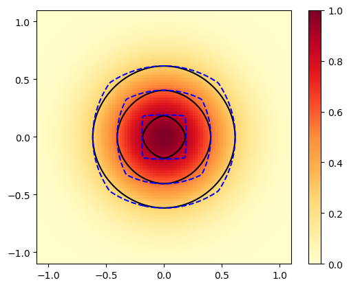
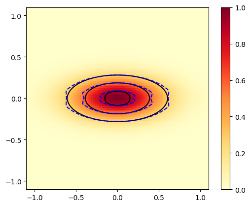
Figure 1: Tests of the eikonal equation. By adopting an explicitly spherical (top) or ellipsoidal (bottom) source, we compare the numerically obtained solution with an analytic solution on the $z=0$ plane. Shown in colormap is the analytic function $u(x,y,0)$ of Eq. 63 while the solid contours represent the numerical solution obtained from solving the flat eikonal equation Eq. 52. The numerical solution agrees very well with the analytic solution and maintains the same symmetry. For comparison, we also include the contours (dashed) obtained with the scheme implemented in HAD from Paper I, which is largely in agreement despite some irregularities along the diagonals.

IV.2 Magnetized, neutron star (cold)

We evolve an isolated, magnetized star using the LS220 EoS and compare the dominant oscillation frequencies with previous work. In particular, we construct a star of (gravitational) mass $1.72M_{\odot}$ with temperature $T=0.01$ MeV and assume beta-equilibrium to set $Y_{e}$. We perturb the star by adding a purely poloidal magnetic field with maximum magnitude $8\times 10^{14}$ G and evolve with a constant initial temperature of $T=0.05$ MeV, slightly higher than that at which it was constructed (but still much smaller than its Fermi energy). The star is evolved within a coarse-level domain spanning $[-150\mathrm{km},150\mathrm{km}]^{3}$ with four total levels of refinement achieving a finest level covering the entire star with a gridspacing of $\Delta x_{\mathrm{min}}=144$ m.

In Fig. 2 we plot changes to the central pressure and magnetic field along with the associated Fourier power spectral densities. Despite some initial transient stage, these central quantities maintain a steady average values avoiding excessive drift. The three dominant oscillation frequencies agree well with those obtained in Paper I and other works using non-linear perturbation theory.

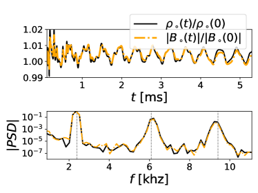
Figure 2: Perturbed, cold star with the LS220 EoS. The top panel shows the variations in central density, $\rho_{0}(t)/\rho_{0}(0)$, and in central magnetic field magnitude, $|B_{0}(t)|/|B_{0}(0)|$. The bottom panel shows the (normalized) power-spectral-density of the quantities in the top panel. The domain of this evolution spans $\left[-150\mathrm{km},150\mathrm{km}\right]^{3}$ with finest resolution $\Delta x_{\mathrm{min}}=144$ m. The reference frequencies noted in Table I of Paper 1 are shown with vertical, dashed, gray lines. Comparing to Fig. 4 of Paper I, the peak frequencies agree quite well.

IV.3 Rotating, magnetized neutron star (hot)

We construct a hot, rotating, magnetized star and evolve with and without neutrino cooling. In particular, we construct a $2.1M_{\odot}$ star spinning at $730$ Hz with an initial temperature of $12$ MeV described by the HShen EoS in beta equilibrium. The initial strength of the magnetic field at the center of the star is $|B_{\circ}|=1.8\times 10^{17}$ G. The computational grid is identical to that described in the previous section for the cold star.

In Fig. 3, we plot the maximum density and temperature versus time for evolutions of this star. Included in the plot is the result of the standard, unmagnetized evolution along with those of evolutions including leakage and both leakage and an initially poloidal magnetic field. As expected the maximum density (generally occurring at the center of the star) hardly depends on effects from the magnetic field and neutrino cooling. In contrast, the maximum temperature decreases faster for those runs including neutrino cooling as would be expected. However, this cooling is happening far from the central region of the star where the temperatures for the different runs are nearly identical. The optical depth decreases toward the surface (snapshots of the optical depths are shown in Fig. 4), allowing the neutrinos to escape. The magnetization, even at this high level, has essentially no effect on the total neutrino luminosity.

We display snapshots along the equatorial plane at $t=5.3$ ms of the star in Fig. 4. The optical depth and vertical component of the magnetic field are very circular, retaining the initial, axisymmetric structure of the star. The emission rates of the different species of neutrinos are also shown, with most of the emission occurring near the surface. These results show that the code maintains the stable, rotating star with neutrino cooling and magnetization present.

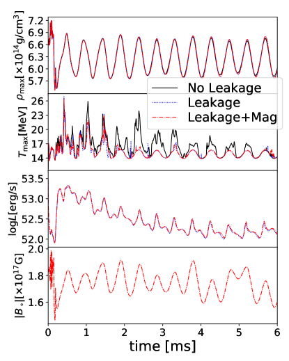
Figure 3: Hot, rapidly rotating star. A $2.1M_{\odot}$ (baryonic) star spinning at $730$ Hz with an initial temperature of $12$ MeV. The maximum density and maximum temperature are shown for all evolutions in the top two panels. The total neutrino luminosity for all species and central magnetic field strength are shown for the evolutions using leakage and with a magnetic field, respectively. With the leakage active, the star cools faster, as expected. An initial magnetization, even very large, has only a very small effect, also as expected. Snapshots of this star at $t=5.26$ ms are shown in Fig. 4.

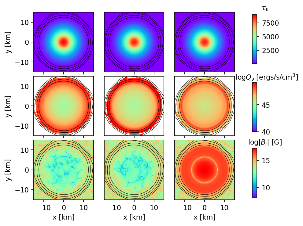
Figure 4: Hot, rapidly rotating star at late time ($t=5.26$ ms). From left to right are shown: Top: Optical depths for $\nu_{e}$, $\bar{\nu}_{e}$, and $\nu_{x}$, Middle: The neutrino luminosities $Q_{e}$, $Q_{a}$, and $Q_{x}$, and Bottom: The magnetic field components, $B_{x}$, $B_{y}$, and $B_{z}$. all along the equatorial plane. The time evolution for this magnetized star with leakage is shown in (red, dotted line) Fig. 3. The contour lines display constant density surfaces at $\log(\rho)=(10.5,11,12,13)\mathrm{g/cm}^{3}$.

IV.4 Binary neutron star merger

We conclude these results with a study of the coalescence of a binary neutron star system. In particular, we choose the same binary studied in Paper I, which uses the SH tabulated equation of state to enable easy comparison. We also investigate possible differences in the neutrino dynamics induced by the strong magnetic field produced during the merger, whose amplification is better captured by the LES.

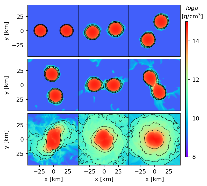
Figure 5: Binary neutron star with SH EoS. Snapshots of the density at various times $t=(0,1.92,3.84,5.76,7.68,9.6,11.52,13.44,18.24)$ms during the coalescence. Notice that the variations due both to the neutrino dynamics and by the magnetic field occur only from the merger onward. The contours display constant density surfaces at $\log\rho=(10.5,11,12,13)\mathrm{g/cm}^{3}$. The stars first make contact around the time $t=9.5$ms (i.e., close to the middle-right panel), and the remnant fluid has largely circularized by the latest time shown (almost $9$ ms after merger).

The initial data for the binary is constructed using the LORENE library, such that each star has baryonic mass $M_{B}=1.49M_{\odot}$ with a cold temperature of $T=0.01$ MeV. The binary has initial separation $45$ km, total ADM mass $M_{\mathrm{ADM}}=2.74M_{\odot}$, and orbital angular velocity $\Omega=1796\,\mathrm{rad\,s}^{-1}$. The electron fraction is set so that the stars are initially in $\beta$-equilibrium.

An old neutron star binary like what we model here is expected to be cold with, at most, a modest magnetic field. Our choice to set the stars at an initial temperature of $0.01$ MeV is consistent with this expectation and near the minimum temperature present in the EoS tables. Despite beginning cold, the stars reach much higher temperatures during merger due to shock heating and other processes. Similarly, the magnetic field, unless extraordinarily large, has essentially no effect during the early inspiral. During merger however, the magnetic field grows and can have significant dynamical effects, particularly on ejecta.

Our binary simulations are evolved in a domain spanning $[-768\mathrm{km},768\mathrm{km}]^{3}$, using adaptive mesh refinement with the finest grid spacing $\Delta x_{\mathrm{min}}=187$m covering the regions with density $\rho\geq 10^{13}\mathrm{g}/\mathrm{cm}^{3}$. The other refinement meshes have increasingly larger sizes, but with coarser resolutions (i.e., by a factor of either 4 or 2, chosen with parameters). The inspiral proceeds as expected, performing approximately 3.5 orbits before merger, as shown in the density snapshots on the equatorial plane displayed in Fig. 5.

Although we compare our results to those obtained in Paper I, the MHDuet code incorporates LES techniques with the gradient SGS model (i.e., with all the coefficients set to zero except the one corresponding to the magnetic field $C_{M}=1/2$) to faithfully capture the amplification of the magnetic field during the merger with moderately high grid resolutions, which our previous HAD code did not. We note again that this comparison will allow us to estimate the effect of magnetic fields on the neutrino-driven dynamics during the first milliseconds after the merger.

The dynamics of the magnetic field evolution can be observed in Fig. 6, where the field intensity and iso-density contours are displayed in the orbital plane for the standard simulation (top row) and the one with LES (bottom row). A thin, rotating shear layer arises at the time of the merger between the stars, prone to develop vortices at small scales induced by the Kelvin-Helmholtz instability. The LES case is able to capture more faithfully the amplification of the magnetic field, as observed qualitatively in Fig. 6. A more quantitative analysis is performed in Fig. 7, which displays the average magnetic field in the star, defined as

$${<}B{>}=\frac{\int|B|\,dV}{\int dV},$$ (65)

where the integration is restricted to regions where the mass density is above $10^{13}\,{\rm g/cm^{3}}$. Clearly in the LES simulation, the magnetic field gets amplified by almost 2 orders of magnitude with respect to the standard simulation during the first milliseconds after the merger. Notice that this large difference is reduced at late times, a result that has been observed previously when using medium-low resolutions like the ones considered here Aguilera-Miret:2020dhz ; 2021arXiv211208413P .

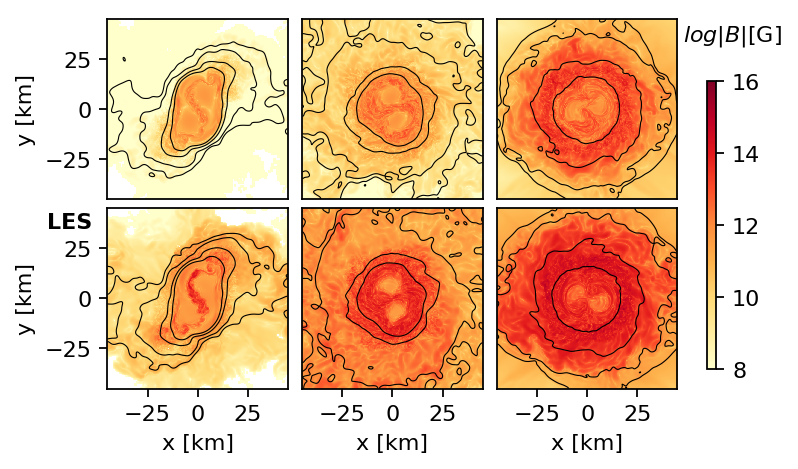
Figure 6: Binary neutron star with SH EoS. Snapshots of the magnetic field strength, and the same constant density iso-surfaces as in Fig. 5, after the merger at times $t=(11.52,13.44,18.24)$ms. The top row corresponds to the standard simulation while the bottom row shows the one with LES. Both simulations incorporate the leakage scheme.

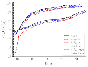
Figure 7: Binary neutron star with SH EoS. Average magnetic field strength as a function of time, starting approximately at the merger, for the standard simulation and the LES. Clearly, the magnetic field grows faster and reaches higher values with the LES, even though these simulations employ only medium resolution (see for instance Fig. 5 in Ref.2021arXiv211208413P to see the effect of the resolution on LES).

The neutrino emission and transport are dominated by the matter density, temperature, and electron fraction. Fig. 8 displays the temperature (in MeV) and the electron fraction, together with the resulting emission rates (in erg/s/cm³) at the final time of our simulations. We observe no qualitative differences between the standard simulation in the top row and the case with LES at the bottom, indicating that the magnetic field is not affecting significantly the dynamics of the neutrinos, except maybe by some small de-phasing. Again, a more quantitative analysis can be performed by computing the luminosity for each neutrino species, displayed in Fig. 9. These luminosities similarly show no significant difference between the standard and the LES cases.

Here, we initialize the stellar field with realistic values $B\leq 10^{12}$G, which might increase during the merger due to different MHD processes. On the other hand, in Paper I (and most work by other authors) a much larger magnetic field was set $B\geq 10^{15}$G. Here, the magnetic field grows to large values, but this growth takes time. In addition, the magnetic field that develops a few milliseconds after merger differs significantly. The field of Paper I retains large scale structure even after merger, but the growth of the magnetic field here develops via small scale turbulence with equipartition between toroidal and poloidal components. Its lack of significant large scale structure minimizes many MHD processes such as the magneto-rotational instability (MRI).

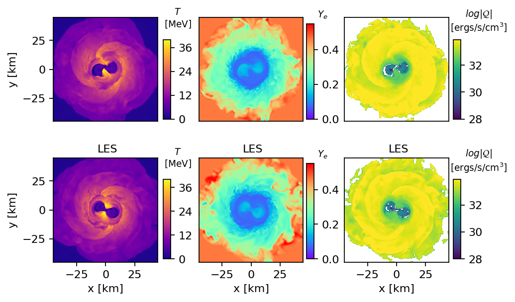
Figure 8: Binary neutron star with SH EoS. Snapshots of the temperature (left), electron fraction (middle) and neutrino emission rates (right) at the final time of the simulation $t=18.24$ ms, approximately 9 ms after the merger. The top row corresponds to the standard simulation, while the bottom row shows the LES case. Both of them include magnetic field, although with LES it is much stronger. Notice that the main difference is a small de-phasing between these two simulations, possibly due to the stronger magnetic field.

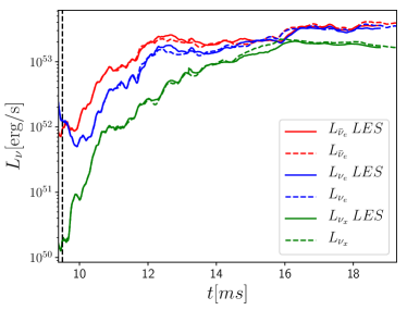
Figure 9: Binary neutron star with SH EoS. Luminosities of the different neutrino species as functions of time, starting approximately at the merger for both the standard simulation and the LES. Again, both of them are for stars with magnetic field. The much stronger magnetic field (roughly two orders of magnitude larger) of the LES simulation arising from its amplification during the turbulent phase of the merger produces only small deviations in the neutrino dynamics compared to the standard, magnetized simulation.

Finally, we compare the resulting gravitational waves in Fig.10. The gravitational radiation is described in terms of the Newman-Penrose scalar $\Psi_{4}$, which can be expanded in terms of spin-weighted $s=-2$ spherical harmonics rezbish ; brugman , namely

$$r\Psi_{4}(t,r,\theta,\phi)=\sum_{l,m}C_{l,m}(t,r)\,Y^{-2}_{l,m}(\theta,\phi).$$ (66)

The coefficients $C_{l,m}$ are extracted from spherical surfaces at a radius $r_{\mathrm{ext}}=300$ km. Only a small de-phasing at late times between the two simulations can be observed, which might suggest some non-negligible effects of the magnetic field braking the remnant.

Because of the importance of the gravitational waveform and its global nature, we study the convergence of this signal for three different resolutions. We consider the standard run discussed above, and run it with a finer grid and a less resolved grid such that the resolution is decreased by a factor of $1.25$ with each step down in resolution. We show the dominant mode $C_{2,2}$ in Fig. 11 along with the differences between successive resolutions. We also display the differences in the phase of the signals. By rescaling the finer difference by the factor expected for third order convergence, we see that the differences indicate at least third order convergence, as expected from previous versions of this code.

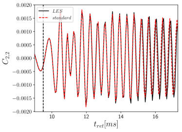
Figure 10: Binary neutron star with SH EoS. Main mode of the gravitational waveform as a function of the retarded time (i.e., subtracting the traveling time of the wave to the surface where it is computed), starting approximately at the merger, for the standard simulation and the LES. Again, no significant differences are observed due to the presence of strong magnetic fields.

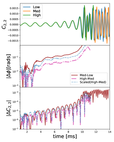
Figure 11: Convergence test of the binary GW signal. The primary mode $C_{2,2}$ for three different resolutions of the binary evolution (top). The medium and low resolutions differ from the high resolution by factors of $1.25$ and $\left(1.25\right)^{2}$. The differences in the phase of the signals (middle) and the absolute differences in the signals (bottom), both measures of the error, are shown, as is the rescaled difference expected between the higher two resolutions if the code converges to third order. The phase appears to converge better than third order while the simple differences in $C_{2,2}$ appear convergent at third order. The medium resolution shown here is the run whose results are presented in the previous figures.

V Conclusions

Here, we present the results of our extension of the MHDuet code, an independent implementation of the fully relativistic magnetohydrodynamics equations mhduet_webpage . The code is generated by the open-source software SIMFLOWNY, and runs under the mature SAMRAI infrastructure, which has been shown to reach exascale for simple problems. We have added both large eddy simulation (LES) methods developed to study the magnetic field amplification that occurs in the turbulent merger regime and a simplified neutrino transport via a leakage scheme. We present details about the adopted methods as well as tests of the code. Although simplified, the leakage scheme will soon be followed by more advanced approximations to model the neutrinos in combination with LES techniques.

For the sake of completeness, we have summarized the evolution equations that are solved for the space-time, the fluid, and the neutrinos, as well as the modifications needed for the LES with the sub-grid-scale gradient model. We have explained in detail the required steps to extend our formalism to microphysical, tabulated equations of state. Finally, we have reviewed the leakage scheme and how to calculate efficiently the optical depth of the neutrinos. In particular, we present two novel additions in this paper: (i) the extension of the gradient SGS model to realistic EoS and (ii) a more formal approximation to resolve the eikonal equation for the optical depth, which preserves well the symmetries of the problem.

We have performed several tests of the code, focusing on the new additions. We have found that the new solver for the eikonal equation is more accurate along diagonals than the original naive method. We have reproduced the oscillation modes of both cold and hot stars with realistic EoS, and also computed the luminosity of the neutrinos in such case. Finally, we have repeated a binary coalescence from Paper I, including both LES and leakage. Our findings indicate that the magnetic field does not affect significantly the dynamics of the neutrinos. Overall, we assess that the code is correct and agrees with previous results from other codes. The core of MHDuet , including its treatment of adaptive mesh boundaries, finite difference methods, and general approach to solving hyperbolic problems, is quite flexible and has already been applied to other problems such as boson star mergers Bezares:2022obu and an alternative theory of gravity PhysRevLett.128.091103 .

As previously mentioned, we plan to extend MHDuet to account for neutrinos in a more realistic way, using the M1 truncated-moments formalism with the Minerbo closure. Such an approach provides for neutrino absorption which has been shown to be important for a proper characterization of the secular ejecta from neutron star mergers. In addition, moment methods go much further than the leakage scheme with actual directional transport and scattering, which become increasingly important with longer evolutions of the post-merger.

Further studies with higher resolutions and with a realistic EoS chosen consistent with the latest observations from LIGO and Virgo Abbott:2018exr and NICER Bogdanov_2019 are needed to study the subtle effects of the magnetic field and neutrino dynamics on multi-messenger observables. In particular, with initial data consistent with GW170817, we plan to examine effects from the magnetic amplification during merger on angular momentum transfer and secular ejecta during the post-merger. Although GW170817 was a “golden” event and perhaps unique, we can hope that similar, close neutron star merger events will be observed in gravitational and electromagnetic bands, especially once third generation detectors come online.

Appendix A Extending SGS model to generic EoS

Here we extend the gradient SGS tensors from Refs. Carrasco:2019uzl ; Vigano:2020ouc , valid for EoS of the form $p=p(\rho,\epsilon)$, in order to accommodate the additional variables $Y_{e}$ and $D_{Y}$ (primitive and conserved, respectively) required for a general EoS $p=p(\rho,\epsilon,Y_{e})$. We follow the same notation as in Ref. Carrasco:2019uzl , where $C^{a}$ denotes the set of conserved evolved variables and $P^{a}$ is the set of primitive fields. Besides the new SGS tensor $H_{N_{Y}}^{k}$, the only other modification of the previous results arises in the term $H_{p}\equiv\nabla\frac{dp}{dC^{a}}\cdot\nabla C^{a}$ from the new dependence on the pressure, i.e., $p(\rho,\epsilon,Y_{e})$

$$\frac{dp}{dC^{a}}=\frac{d{p}}{d{\rho}}\frac{d{\rho}}{d{C^{a}}}+\frac{d{p}}{d{\epsilon}}\frac{d{\epsilon}}{d{C^{a}}}+\frac{d{p}}{d{Y_{e}}}\frac{d{Y_{e}}}{d{C^{a}}}.$$ (67)

The only non-zero additional elements of the Jacobian (conserved-to-primitive) $dC^{a}/dP^{b}$ and its inverse $dP^{a}/dC^{b}$ are, respectively,

$$\frac{dD_{Y}}{dY_{e}}=D\quad\text{, }\quad\frac{dD_{Y}}{dP^{a^{\prime}}}=Y_{e}\frac{dD}{dP^{a^{\prime}}}$$

$$\frac{dY_{e}}{dD_{Y}}=\frac{1}{D}\quad\text{, }\quad\frac{dY_{e}}{dD}=-\frac{Y_{e}}{D},$$

where $P^{a^{\prime}}$ denote the “old” set of primitive variables (i.e., excluding $Y_{e}$) and $C^{a^{\prime}}$ the “old” set of conserved variables (i.e., excluding $D_{Y}$). Hence, we note that the new variables are only partially coupled to the system through the field $D$. In particular, we note that $d{\rho}/d{D_{Y}}=d{\epsilon}/d{D_{Y}}=0$. We can now compute (67) and, therefore, obtain the following new expression for $H_{p}$

$$H_{p} = \nabla\left(\frac{d{p}}{d{\rho}}\frac{d{\rho}}{d{C^{a^{\prime}}}}+\frac{d{p}}{d{\epsilon}}\frac{d{\epsilon}}{d{C^{a^{\prime}}}}\right)\cdot\nabla C^{a^{\prime}}+\nabla\left(\frac{d{p}}{d{Y_{e}}}\frac{d{Y_{e}}}{d{C^{a}}}\right)\cdot\nabla C^{a}$$ (68)

$$= H^{\rm old}_{p}+\nabla\left(\frac{1}{D}\frac{d{p}}{d{Y_{e}}}\right)\cdot\nabla D_{Y}-\nabla\left(\frac{Y_{e}}{D}\frac{d{p}}{d{Y_{e}}}\right)\cdot\nabla D$$

$$= H^{\rm old}_{p}+\nabla\frac{d{p}}{d{Y_{e}}}\cdot\nabla Y_{e}-\frac{2}{D}\frac{d{p}}{d{Y_{e}}}\nabla Y_{e}\cdot\nabla D.$$

where $H^{\mathrm{old}}$ was the expression obtained for the EoS $p=p(\rho,\epsilon)$.

Appendix B Numerical schemes

Here we present an overview of the numerical schemes (i.e., the time integrator and the spatial discretization for smooth and for non-smooth solutions) available in Simflowny and their implementation in the SAMRAI infrastructure.

We employ the Method of Lines to separate the time from the space discretization. Within this approach, the time integration of the equations is performed with the standard fourth order Runge-Kutta (RK), that is written in the standard Butcher form in Table 1.

Table 1: Butcher tableau for the standard explicit fourth-order RK (with four sub-steps).

0	0	0	0	0
1/2	1/2	0	0	0
1/2	0	1/2	0	0
1	0	0	1	0
	1/6	2/6	2/6	1/6

The spatial discretization of the Einstein equations is performed using fourth-order, centered, finite differences. For some quantity $U_{i,j,k}$ defined at a gridpoint $(x_{i},y_{j},z_{k})$, we present the operators used to compute derivatives along the $x$-axis with similar expressions for derivatives along the $y$- and $z$-axes. The first order derivative operators can be written as

$$\partial_{x}U_{i,j,k} = \frac{1}{12\Delta x}\left(U_{i-2,j,k}-8\,U_{i-1,j,k}\right.$$ (69)

$$+ \left.8\,U_{i+1,j,k}-U_{i+2,j,k}\right)+{\cal O}(\Delta x^{4}).$$

The second order derivative is

$$\partial_{xx}U_{i,j,k} = \frac{1}{12\Delta x^{2}}\left(-U_{i-2,j,k}+16\,U_{i-1,j,k}-30\,U_{i,j,k}\right.$$ (70)

$$+ \left.16\,U_{i+1,j,k}-U_{i+2,j,k}\right)+{\cal O}(\Delta x^{4}).$$

The second order, mixed derivatives are obtained by applying the first order derivative operator twice. For instance, the $xy$-derivative would be just

$$\partial_{xy}U_{i,j,k} = \partial_{x}\left(\partial_{y}U_{i,j,k}\right)=\partial_{y}\left(\partial_{x}U_{i,j,k}\right).$$ (71)

We use centered derivative operators for all the derivative terms except for the advection terms, which are generically proportional to the shift vector $\beta^{i}$. In those cases, we use one-sided derivative schemes depending on the sign of the shift, namely

$$\partial_{x}U_{i,j,k}=\begin{dcases}&\frac{1}{12\Delta x}\left(-U_{i-3,j,k}+6\,U_{i-2,j,k}-18\,U_{i-1,j,k}\right.\\ &+\left.10\,U_{i,j,k}+3\,U_{i+1,j,k}\right)~{}~{}\text{if }~{}~{}\beta^{x}<0\\ &\frac{1}{12\Delta x}\left(U_{i+3,j,k}-6\,U_{i+2,j,k}+18\,U_{i+1,j,k}\right.\\ &-\left.10\,U_{i,j,k}-3\,U_{i-1,j,k}\right)~{}~{}\text{if }~{}~{}\beta^{x}\geq 0.\end{dcases}$$

A small amount of artificial dissipation is applied to the spacetime fields in order to filter the high frequency modes of the solution which are not truly represented in our numerical grid (i.e., their wavelength is smaller than the grid size $\Delta x$). We use the Kreiss-Oliger dissipation operator SBP3 that preserves the accuracy of our fourth-order operators and takes the form (i.e., for instance along the x-direction) (again, written in terms of the $x$-direction)

$$Q^{x}_{d}U_{i,j,k} = \sigma(\Delta x)^{5}\left(D^{x}_{+}\right)^{3}\left(D^{x}_{-}\right)^{3}U_{i,j,k}$$

$$= \frac{\sigma}{64\Delta x}\left(U_{i-3,j,k}-6\,U_{i-2,j,k}+15\,U_{i-1,j,k}\right.$$

$$- \left.20\,U_{i,j,k}+15\,U_{i+1,j,k}-6\,U_{i+2,j,k}+U_{i+3,j,k}\right)$$

where $\sigma\geq 0$ is the dissipation parameter.

The MHD equations are written in conservation law form

$$\partial_{t}{\bf U}+\partial_{k}F^{k}({\bf U})=S({\bf U})$$ (73)

where ${\bf U}$ is the vector of evolved fields and $F^{k}({\bf U})$, $S({\bf U})$ their corresponding fluxes and sources, which might be non-linear but depend only on the fields and not on their derivatives. This form of the equation allows us to use High-Resolution-Shock-Capturing (HRSC) methods (Toro:1997, ) to deal with the possible appearance of shocks and to take advantage of the existence of weak solutions in the equations.

A discrete conservative scheme of Eq. (73) (i.e., the change of the cell average is given by the difference in fluxes across the boundary of the cell) can be obtained by approximating the derivatives of the fluxes, for instance along the x-direction, as follows

$$\partial_{x}F\approx\frac{1}{\Delta x}(\hat{F}_{i+1/2}-\hat{F}_{i-1/2})$$ (74)

where the problem consists of finding a non-oscillatory, high-order approximation to the interface values of $\hat{F}_{i+1/2}$. Thus one can set $\hat{F}_{i+1/2}=R(F_{[s]})$, where $R()$ is a highly accurate reconstruction scheme providing a stable interface flux value from point-wise neighboring values, while the index $[s]$ spans through the interpolation stencil. The crucial issue in HRSC methods is how to approximate the solution of the Riemann problem, by reconstructing the fluxes at the interfaces with information from the left(L) and the right(R) states such that no spurious oscillations appear in the solutions.

We consider the following combination of the fluxes and the fields, at each gridpoint $x_{i}$,

$$F^{\pm}_{i}=\frac{1}{2}\left(F_{i}\pm\lambda U_{i}\right)$$ (75)

where $\lambda$ is the maximum propagation speed of the system in the neighboring points. Then, from the neighboring nodes $\{x_{i-n},..,x_{i+1+n}\}$ (i.e., where $n$ is the width of the stencil), we reconstruct the fluxes at the left and right of each interface as

$$F^{L}_{i+1/2}=R(\{F^{+}\})~{}~{},~{}~{}F^{R}_{i+1/2}=R(\{F^{-}\}).$$ (76)

The number $2(n+1)$ of such neighbors used in the reconstruction procedure depends on the order of the method. Simflowny already incorporates some commonly used reconstructions, such as Piecewise Parabolic Method (PPM) Colella:1982ee , the Weighted-Essentially-Non-Oscillatory (WENO) reconstruction methods Jiang:1996 ; Shu:1998 , and the fifth order Monotonic-Preserving scheme (MP5) suresh97 , as well as other implementations such as the Finite-Difference Osher-Chakravarthy (FDOC) families Bona:2009 . We typically use the MP5 scheme in our code MHDuet .

We use a flux formula to compute the final flux at each interface as

$$\hat{F}_{i+1/2}=F^{L}_{i+1/2}+F^{R}_{i+1/2}.$$ (77)

Note that this reconstruction method does not require the characteristic decomposition of the system of equations (i.e., the full spectrum of characteristic velocities).

References

- (1) B. P. Abbott, R. Abbott, T. D. Abbott, F. Acernese, K. Ackley, C. Adams, T. Adams, P. Addesso, R. X. Adhikari, V. B. Adya, C. Affeldt, M. Afrough, B. Agarwal, M. Agathos, K. Agatsuma, and N. Aggarwal, “Multi-messenger observations of a binary neutron star merger,” The Astrophysical Journal Letters 848 no. 2, (2017) L12. http://stacks.iop.org/2041-8205/848/i=2/a=L12.
- (2) LIGO Scientific Collaboration and Virgo Collaboration Collaboration, B. P. Abbott et al., “Gw170817: Observation of gravitational waves from a binary neutron star inspiral,” Phys. Rev. Lett. 119 (Oct, 2017) 161101. https://link.aps.org/doi/10.1103/PhysRevLett.119.161101.
- (3) A. Balasubramanian, A. Corsi, K. P. Mooley, M. Brightman, G. Hallinan, K. Hotokezaka, D. L. Kaplan, D. Lazzati, and E. J. Murphy, “Continued Radio Observations of GW170817 3.5 yr Post-merger,” Astrophys. J. Lett. 914 no. 1, (2021) L20, arXiv:2103.04821 [astro-ph.HE].
- (4) D. Radice, S. Bernuzzi, and A. Perego, “The Dynamics of Binary Neutron Star Mergers and GW170817,” Ann. Rev. Nucl. Part. Sci. 70 (2020) 95–119, arXiv:2002.03863 [astro-ph.HE].
- (5) R. Ciolfi, “Binary neutron star mergers after GW170817,” Front. Astron. Space Sci. 7 (2020) 27, arXiv:2005.02964 [astro-ph.HE].
- (6) J. Barnes, “The Physics of Kilonovae,” Front. in Phys. 8 (2020) 355.
- (7) R. Ciolfi, “The key role of magnetic fields in binary neutron star mergers,” General Relativity and Gravitation 52 no. 6, (June, 2020) 59, arXiv:2003.07572 [astro-ph.HE].
- (8) F. Foucart, P. Laguna, G. Lovelace, D. Radice, and H. Witek, “Snowmass2021 Cosmic Frontier White Paper: Numerical relativity for next-generation gravitational-wave probes of fundamental physics,” arXiv:2203.08139 [gr-qc].
- (9) C. Pacilio, A. Maselli, M. Fasano, and P. Pani, “Ranking the Love for the neutron star equation of state: the need for third-generation detectors,” arXiv:2104.10035 [gr-qc].
- (10) J. C. McKinney and R. D. Blandford, “Stability of relativistic jets from rotating, accreting black holes via fully three-dimensional magnetohydrodynamic simulations,” Monthly Notices of the Royal Astronomical Society: Letters 394 no. 1, (Mar, 2009) L126–L130. http://dx.doi.org/10.1111/j.1745-3933.2009.00625.x.
- (11) M. Liska, A. Tchekhovskoy, and E. Quataert, “Large-scale poloidal magnetic field dynamo leads to powerful jets in GRMHD simulations of black hole accretion with toroidal field,” Monthly Notices of the Royal Astronomical Society 494 no. 3, (04, 2020) 3656–3662, https://academic.oup.com/mnras/article-pdf/494/3/3656/33145099/staa955.pdf. https://doi.org/10.1093/mnras/staa955.
- (12) M. Ruiz, A. Tsokaros, and S. L. Shapiro, “Magnetohydrodynamic simulations of binary neutron star mergers in general relativity: Effects of magnetic field orientation on jet launching,” Phys. Rev. D 101 (Mar, 2020) 064042. https://link.aps.org/doi/10.1103/PhysRevD.101.064042.
- (13) P. Mösta, D. Radice, R. Haas, E. Schnetter, and S. Bernuzzi, “A Magnetar Engine for Short GRBs and Kilonovae,” ApJL 901 no. 2, (Oct., 2020) L37, arXiv:2003.06043 [astro-ph.HE].
- (14) F. Foucart, M. D. Duez, F. Hebert, L. E. Kidder, H. P. Pfeiffer, and M. A. Scheel, “Monte-Carlo Neutrino Transport in Neutron Star Merger Simulations,” ApJL 902 no. 1, (Oct., 2020) L27, arXiv:2008.08089 [astro-ph.HE].
- (15) D. Radice, S. Bernuzzi, A. Perego, and R. Haas, “A new moment-based general-relativistic neutrino-radiation transport code: Methods and first applications to neutron star mergers,” MNRAS 512 no. 1, (May, 2022) 1499–1521, arXiv:2111.14858 [astro-ph.HE].
- (16) D. Neilsen, S. L. Liebling, M. Anderson, L. Lehner, E. O’Connor, et al., “Magnetized Neutron Stars With Realistic Equations of State and Neutrino Cooling,” Phys.Rev. D89 (2014) 104029, arXiv:1403.3680 [gr-qc].
- (17) C. Palenzuela, S. Liebling, D. Neilsen, L. Lehner, O. Caballero, et al., “Effects of the microphysical Equation of State in the mergers of magnetized Neutron Stars With Neutrino Cooling,” arXiv:1505.01607 [gr-qc].
- (18) E. R. Most, L. J. Papenfort, and L. Rezzolla, “Beyond second-order convergence in simulations of magnetized binary neutron stars with realistic microphysics,” MNRAS 490 no. 3, (Dec., 2019) 3588–3600, arXiv:1907.10328 [astro-ph.HE].
- (19) F. Cipolletta, J. V. Kalinani, E. Giangrandi, B. Giacomazzo, R. Ciolfi, L. Sala, and B. Giudici, “Spritz: general relativistic magnetohydrodynamics with neutrinos,” Classical and Quantum Gravity 38 no. 8, (Apr., 2021) 085021, arXiv:2012.10174 [astro-ph.HE].
- (20) L. Sun, M. Ruiz, S. L. Shapiro, and A. Tsokaros, “Jet Launching from Binary Neutron Star Mergers: Incorporating Neutrino Transport and Magnetic Fields,” arXiv e-prints (Feb., 2022) arXiv:2202.12901, arXiv:2202.12901 [astro-ph.HE].
- (21) F. Carrasco, D. Viganò, and C. Palenzuela, “Gradient sub-grid-scale model for relativistic MHD Large Eddy Simulations,” arXiv:1908.01419 [astro-ph.HE].
- (22) D. Viganò, R. Aguilera-Miret, F. Carrasco, B. Miñano, and C. Palenzuela, “General relativistic MHD large eddy simulations with gradient subgrid-scale model,” Phys. Rev. D 101 no. 12, (2020) 123019, arXiv:2004.00870 [gr-qc].
- (23) R. Aguilera-Miret, D. Viganò, F. Carrasco, B. Miñano, and C. Palenzuela, “Turbulent magnetic-field amplification in the first 10 milliseconds after a binary neutron star merger: Comparing high-resolution and large-eddy simulations,” Phys. Rev. D 102 no. 10, (2020) 103006, arXiv:2009.06669 [gr-qc].
- (24) C. Palenzuela, R. Aguilera-Miret, F. Carrasco, R. Ciolfi, J. V. Kalinani, W. Kastaun, B. Miñano, and D. Viganò, “Turbulent magnetic field amplification in binary neutron star mergers,” arXiv e-prints (Dec., 2021) arXiv:2112.08413, arXiv:2112.08413 [gr-qc].
- (25) R. Aguilera-Miret, D. Viganò, and C. Palenzuela, “Universality of the Turbulent Magnetic Field in Hypermassive Neutron Stars Produced by Binary Mergers,” ApJL 926 no. 2, (Feb., 2022) L31, arXiv:2112.08406 [gr-qc].
- (26) S. L. Liebling, C. Palenzuela, and L. Lehner, “Effects of High Density Phase Transitions on Neutron Star Dynamics,” Class. Quant. Grav. 38 no. 11, (2021) 115007, arXiv:2010.12567 [gr-qc].
- (27) L. Lehner, S. L. Liebling, C. Palenzuela, O. L. Caballero, E. O’Connor, M. Anderson, and D. Neilsen, “Unequal mass binary neutron star mergers and multimessenger signals,” Class. Quant. Grav. 33 no. 18, (2016) 184002, arXiv:1603.00501 [gr-qc].
- (28) C. Palenzuela, B. Miñano, D. Viganò, A. Arbona, C. Bona-Casas, A. Rigo, M. Bezares, C. Bona, and J. Massó, “A Simflowny-based finite-difference code for high-performance computing in numerical relativity,” Class. Quant. Grav. 35 no. 18, (2018) 185007, arXiv:1806.04182 [physics.comp-ph].
- (29) D. Viganò, D. Martínez-Gómez, J. A. Pons, C. Palenzuela, F. Carrasco, B. Miñano, A. Arbona, C. Bona, and J. Massó, “A Simflowny-based high-performance 3D code for the generalized induction equation,” arXiv:1811.08198 [astro-ph.IM].
- (30) S. L. Liebling, C. Palenzuela, and L. Lehner, “Toward fidelity and scalability in non-vacuum mergers,” Class. Quant. Grav. 37 no. 13, (2020) 135006, arXiv:2002.07554 [gr-qc].
- (31) M. Bezares, C. Palenzuela, and C. Bona, “Final fate of compact boson star mergers,” Phys. Rev. D95 no. 12, (2017) 124005, arXiv:1705.01071 [gr-qc].
- (32) M. Bezares and C. Palenzuela, “Gravitational Waves from Dark Boson Star binary mergers,” Class. Quant. Grav. 35 no. 23, (2018) 234002, arXiv:1808.10732 [gr-qc].
- (33) M. Bezares, M. Bošković, S. Liebling, C. Palenzuela, P. Pani, and E. Barausse, “Gravitational waves and kicks from the merger of unequal mass, highly compact boson stars,” Phys. Rev. D 105 no. 6, (2022) 064067, arXiv:2201.06113 [gr-qc].
- (34) M. Bezares, R. Aguilera-Miret, L. ter Haar, M. Crisostomi, C. Palenzuela, and E. Barausse, “No evidence of kinetic screening in simulations of merging binary neutron stars beyond general relativity,” Phys. Rev. Lett. 128 (Mar, 2022) 091103. https://link.aps.org/doi/10.1103/PhysRevLett.128.091103.
- (35) D. Alic, C. Bona-Casas, C. Bona, L. Rezzolla, and C. Palenzuela, “Conformal and covariant formulation of the Z4 system with constraint-violation damping,” Phys. Rev. D 85 no. 6, (Mar, 2012) 064040, arXiv:1106.2254 [gr-qc].
- (36) M. Alcubierre, B. Brügmann, P. Diener, M. Koppitz, D. Pollney, E. Seidel, and R. Takahashi, “Gauge conditions for long-term numerical black hole evolutions without excision,” Physical Review D 67 no. 8, (Apr, 2003) . http://dx.doi.org/10.1103/PhysRevD.67.084023.
- (37) J. R. van Meter, J. G. Baker, M. Koppitz, and D.-I. Choi, “How to move a black hole without excision: Gauge conditions for the numerical evolution of a moving puncture,” Phys. Rev. D 73 no. 12, (June, 2006) 124011, arXiv:gr-qc/0605030 [gr-qc].
- (38) E. O’Connor and C. D. Ott, “A New Open-Source Code for Spherically-Symmetric Stellar Collapse to Neutron Stars and Black Holes,” Class. Quant. Grav. 27 (2010) 114103, arXiv:0912.2393 [astro-ph.HE].
- (39) F. Galeazzi, W. Kastaun, L. Rezzolla, and J. A. Font, “Implementation of a simplified approach to radiative transfer in general relativity,” Phys. Rev. D 88 no. 6, (Sept., 2013) 064009, arXiv:1306.4953 [gr-qc].
- (40) J. M. Lattimer and F. Douglas Swesty, “A generalized equation of state for hot, dense matter,” Nuclear Physics A 535 (Dec., 1991) 331–376.
- (41) H. Shen, H. Toki, K. Oyamatsu, and K. Sumiyoshi, “Relativistic Equation of State for Core-collapse Supernova Simulations,” ApJS 197 (Dec., 2011) 20, arXiv:1105.1666 [astro-ph.HE].
- (42) M. H. Ruffert, H. T. Janka, and G. Schaefer, “Coalescing neutron stars: A step towards physical models. I: Hydrodynamic evolution and gravitational- wave emission,” Astron. Astrophys. 311 (1996) 532–566, arXiv:astro-ph/9509006.
- (43) S. Rosswog and M. Liebendoerfer, “High resolution calculations of merging neutron stars. 2: Neutrino emission,” Mon.Not.Roy.Astron.Soc. 342 (2003) 673, arXiv:astro-ph/0302301 [astro-ph].
- (44) D. Viganò, R. Aguilera-Miret, and C. Palenzuela, “Extension of the subgrid-scale gradient model for compressible magnetohydrodynamics turbulent instabilities,” Physics of Fluids 31 no. 10, (Oct, 2019) 105102, arXiv:1904.04099 [physics.flu-dyn].
- (45) A. Arbona, A. Artigues, C. Bona-Casas, J. Massó, B. Miñano, A. Rigo, M. Trias, and C. Bona, “Simflowny: A general-purpose platform for the management of physical models and simulation problems,” Computer Physics Communications 184 no. 10, (2013) 2321–2331. http://www.sciencedirect.com/science/article/pii/S0010465513001471.
- (46) A. Arbona, B. Miñano, A. Rigo, C. Bona, C. Palenzuela, A. Artigues, C. Bona-Casas, and J. Massó, “Simflowny 2: An upgraded platform for scientific modelling and simulation,” Computer Physics Communications 229 (2018) 170–181. http://www.sciencedirect.com/science/article/pii/S0010465518300870.
- (47) C. Palenzuela, B. Miñano, A. Arbona, C. Bona-Casas, C. Bona, and J. Massó, “Simflowny 3: An upgraded platform for scientific modeling and simulation,” Computer Physics Communications 259 (2021) 107675. https://www.sciencedirect.com/science/article/pii/S0010465520303271.
- (48) R. D. Hornung and S. R. Kohn, “Managing application complexity in the samrai object-oriented framework,” Concurrency and Computation: Practice and Experience 14 no. 5, (2002) 347–368. http://dx.doi.org/10.1002/cpe.652.
- (49) B. T. Gunney and R. W. Anderson, “Advances in patch-based adaptive mesh refinement scalability,” Journal of Parallel and Distributed Computing 89 (2016) 65–84. http://www.sciencedirect.com/science/article/pii/S0743731515002129.
- (50) C.-W. Shu, Essentially non-oscillatory and weighted essentially non-oscillatory schemes for hyperbolic conservation laws, pp. 325–432. Springer Berlin Heidelberg, Berlin, Heidelberg, 1998. https://doi.org/10.1007/BFb0096355.
- (51) A. Suresh and H. Huynh, “Accurate monotonicity-preserving schemes with runge–kutta time stepping,” Journal of Computational Physics 136 no. 1, (1997) 83 – 99. http://www.sciencedirect.com/science/article/pii/S0021999197957454.
- (52) P. McCorquodale and P. Colella, “A high-order finite-volume method for conservation laws on locally refined grids,” Commun. Appl. Math. Comput. Sci. 6 no. 1, (2011) 1–25. https://doi.org/10.2140/camcos.2011.6.1.
- (53) B. Mongwane, “Toward a Consistent Framework for High Order Mesh Refinement Schemes in Numerical Relativity,” Gen.Rel.Grav. 47 no. 5, (2015) 60, arXiv:1504.07609 [gr-qc].
- (54) P. Cerdá-Durán, J. A. Font, L. Antón, and E. Müller, “A new general relativistic magnetohydrodynamics code for dynamical spacetimes,” A&A 492 no. 3, (Dec., 2008) 937–953, arXiv:0804.4572 [astro-ph].
- (55) D. M. Siegel, P. Mösta, D. Desai, and S. Wu, “Recovery Schemes for Primitive Variables in General-relativistic Magnetohydrodynamics,” ApJ 859 no. 1, (May, 2018) 71, arXiv:1712.07538 [astro-ph.HE].
- (56) J. A. Sethian, “Fast marching methods,” SIAM Review 41 no. 2, (1999) 199–235, https://doi.org/10.1137/S0036144598347059. https://doi.org/10.1137/S0036144598347059.
- (57) A. Chacon and A. Vladimirsky, “Fast two-scale methods for eikonal equations,” SIAM Journal on Scientific Computing 34 no. 2, (2012) A547–A578, https://doi.org/10.1137/10080909X. https://doi.org/10.1137/10080909X.
- (58) N. T. Bishop and L. Rezzolla, “Extraction of gravitational waves in numerical relativity,” Living Reviews in Relativity 19 (Oct., 2016) 2, arXiv:1606.02532 [gr-qc].
- (59) B. Brügmann, J. A. González, M. Hannam, S. Husa, U. Sperhake, and W. Tichy, “Calibration of moving puncture simulations,” Phys. Rev. D 77 no. 2, (Jan., 2008) 024027, gr-qc/0610128.
-
(60)
“MHDuet webpage.”
http://mhduet.liu.edu/, 2022. - (61) Virgo, LIGO Scientific Collaboration, B. P. Abbott et al., “GW170817: Measurements of neutron star radii and equation of state,” arXiv:1805.11581 [gr-qc].
- (62) S. Bogdanov, F. K. Lamb, S. Mahmoodifar, M. C. Miller, S. M. Morsink, T. E. Riley, T. E. Strohmayer, A. K. Tung, A. L. Watts, A. J. Dittmann, D. Chakrabarty, S. Guillot, Z. Arzoumanian, and K. C. Gendreau, “Constraining the neutron star mass–radius relation and dense matter equation of state with NICER. II. emission from hot spots on a rapidly rotating neutron star,” The Astrophysical Journal 887 no. 1, (Dec, 2019) L26. https://doi.org/10.3847%2F2041-8213%2Fab5968.
- (63) G. Calabrese, L. Lehner, O. Reula, O. Sarbach, and M. Tiglio, “Summation by parts and dissipation for domains with excised regions,” Class. Quant. Grav. 21 (2004) 5735–5758, gr-qc/0308007.
- (64) E. Toro, Riemann Solvers and Numerical Methods for Fluid Dynamics: A Practical Introduction. Springer, 1997. https://books.google.es/books?id=6QFAAQAAIAAJ.
- (65) P. Colella and P. R. Woodward, “The piecewise parabolic method (ppm) for gas dynamical simulations,” J. Comput. Phys. 54 (1984) 174–201.
- (66) G.-S. Jiang and C.-W. Shu, “Efficient implementation of weighted eno schemes,” Journal of Computational Physics 126 no. 1, (1996) 202 – 228. http://www.sciencedirect.com/science/article/pii/S0021999196901308.
- (67) C.-W. Shu, Essentially non-oscillatory and weighted essentially non-oscillatory schemes for hyperbolic conservation laws, pp. 325–432. Springer Berlin Heidelberg, Berlin, Heidelberg, 1998. https://doi.org/10.1007/BFb0096355.
- (68) C. Bona, C. Bona-Casas, and J. Terradas, “Linear high-resolution schemes for hyperbolic conservation laws: TVB numerical evidence,” Journal of Computational Physics 228 (Apr., 2009) 2266–2281, arXiv:0810.2185 [gr-qc].