Dynamical state of galaxy clusters evaluated from X-ray images

Abstract

X-ray images of galaxy clusters often show disturbed structures that are indication of cluster mergers. As a complementary to our previous work on dynamical state of 964 clusters observed by the Chandra, we process the X-ray images for 1308 clusters from XMM-Newton archival data, together with the images of 22 clusters newly released by the Chandra, and evaluate their dynamical state from these X-ray images. The concentration index $c$, the centroid shift $\omega$, the power ratio $P_{3}/P_{0}$ are calculated in circular regions with a certain radius of 500 kpc, and the morphology index $\delta$ is estimated within elliptical regions adaptive to the cluster size and shape. In addition, the dynamical parameters for 42 clusters previously estimated from Chandra images are upgraded based on the newly available redshifts. Good consistence is found between dynamical parameters derived from XMM-Newton and Chandra images for the overlapped sample of clusters in the two datasets. The dependence of mass scaling relations on dynamical state is shown by using data of 388 clusters. All data and related software are available on web-page http://zmtt.bao.ac.cn/galaxy_clusters/dyXimages/.

1 Introduction

Clusters of galaxies are in various dynamical states. Some of them are dynamically relaxed, but a large fraction of clusters are not in dynamical equilibrium (e.g., Chon & Böhringer, 2017; Lopes et al., 2018; Yuan & Han, 2020). The dynamical state is a fundamental characteristic of galaxy clusters, in additional to other properties such as the mass or the temperature of intracluster medium (ICM).

The dynamical state of galaxy clusters can be quantitatively figured out by various observational tracers. In optical, it can be roughly indicated by the redshift distribution of member galaxies (e.g., Yahil & Vidal, 1977; Dressler & Shectman, 1988; West & Bothun, 1990; Solanes et al., 1999; Halliday et al., 2004; Hou et al., 2009; Roberts et al., 2018; Yu et al., 2018), which is the 1-dimensional (1D) information along the line of sight. In principle, the dynamical state should be determined by the 3D velocities and mass distributions of all member galaxies and/or ICM (e.g., Colless & Dunn, 1996; Einasto et al., 2010, 2012). However, it is very hard to get the full 3D information in practice. The dynamical state can be well represented with 2D maps, because if a cluster is disturbed in 2D map it must be really disturbed in 3D though information on the radial dimension is missing. Analyses of the 2D position distributions of member galaxies have been tried for many years (e.g., Geller & Beers, 1982; West & Bothun, 1990; Flin & Krywult, 2006; Ramella et al., 2007; Aguerri & Sánchez-Janssen, 2010; Einasto et al., 2012; Wen & Han, 2013; Lopes et al., 2018; Klein et al., 2019). The largest sample of clusters is presented by Wen & Han (2013), who smoothed the optical flux-weighted maps of member galaxies in the sky plane, and calculated the relaxation factor $\Gamma$ for 2092 rich clusters. In X-ray, dynamical parameters of clusters can be obtained by analyzing the images of hot intracluster gas, though calculating the central cooling time (e.g., Bauer et al., 2005; Chen et al., 2007), the concentration index (e.g., Santos et al., 2008; Cuciti et al., 2015; Zhang et al., 2017; Liu et al., 2018), the centroid shift (e.g., Poole et al., 2006; Cassano et al., 2010, 2013; Donahue et al., 2016), the power ratio (e.g., Buote & Tsai, 1995; Weißmann et al., 2013a, b), or simply the morphology index (Yuan & Han, 2020). In microwave band, the dynamical state of clusters can also be derived from maps of Sunyaev-Zel’dovich (SZ) effect (e.g., Cialone et al., 2018).

Previously, high quality X-ray images are difficult to get, therefore dynamical parameters of only a limited sample (generally less than 100) of clusters were calculated (e.g., Buote & Tsai, 1995; Santos et al., 2008; Cassano et al., 2010, 2013; Weißmann et al., 2013a; Donahue et al., 2016; Zhang et al., 2017; Liu et al., 2018). Recent years, the Chandra and the XMM-Newton X-ray telescopes observed many clusters of galaxies. Weißmann et al. (2013b) calculated the power ratios for 129 clusters in the redshift range of $0.05<z<1.08$ from the Chandra and XMM-Newton images. Andrade-Santos et al. (2017) computed the concentration indexes for 214 clusters from Chandra images. Zenteno et al. (2020) derived the offset of brightest cluster galaxies to the brightness peak of hot gas indicated by SZ (SPT) or X-ray (Chandra/XMM-Newton) images for 288 clusters. Yuan & Han (2020) processed the released Chandra images for 964 clusters, and calculated the concentration indexes, the centroid shifts, the power ratios and also the morphology indexes.

The XMM-Newton X-ray telescope has observed more than 1000 clusters of galaxies with a larger field of view than the Chandra. As a continuation of Yuan & Han (2020), we calculate the dynamical parameters for 1308 clusters in the archived XMM-Newton data. In Section 2, we describe the procedures for cluster finding from the data and image processing. In Section 3, dynamical parameters are calculated, not only for these 1308 clusters, but also for clusters newly released by the Chandra. In Section 4, the influence of dynamical state on cluster mass estimation is discussed. Finally, a summary is given in Section 5.

Throughout this paper, the flat $\Lambda$CDM cosmology is adopted with $H_{0}=70$ km s^-1 Mpc^-1, $\Omega_{m}=0.3$ and $\Omega_{\Lambda}=0.7$.

2 Cluster samples and image processing

2.1 Galaxy clusters in X-ray data archives

As in Yuan & Han (2020), we find clusters in the archived data by two approaches: (1) targeted objects in proposed observations for galaxy clusters; and (2) serendipitously detected clusters.

First, in the XMM-Newton Science Archive Search system, we select the proposal category of “Groups of galaxies, Clusters of galaxies and Superclusters”, and find more than 2000 observations. For a cluster with multiple observations, we choose the one with the longest exposure time. For low redshift clusters (e.g., $z<0.05$), the field coverage should also be cared. After checking the raw images, discarding multiple observations and rejecting poor quality data, we get the targeted sample of 892 clusters.

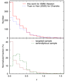
Figure 1: Upper panel: Redshift distribution for 1301 of 1308 galaxy clusters (solid) with available redshift observed by the XMM-Newton, compared to that (short-dashed) for clusters in Yuan & Han (2020) by the Chandra. Lower panel: Redshift distribution for clusters in the targeted sample (solid) and the serendipitous sample (dashed) detected by the XMM-Newton.

Second, we combined several large cluster catalogues (Abell et al., 1989; Piffaretti et al., 2011; Rykoff et al., 2014; Wen et al., 2012; Wen & Han, 2015; Wen et al., 2018; Zou et al., 2021; Koulouridis et al., 2021), and check if any clusters serendipitously observed in XMM-Newton observations in the released dataset. The instrument mode for the MOS1 and MOS2 is set as “full frame”, and the modes “full frame”, “extended full frame” and “large window” are chosen for the EPN sytem. Observations with any filters are adopted. After merging multiple items in outputs, we get a sample of 416 clusters serendipitously detected in any XMM-Newton observations. Together with 892 clusters in the targeted sample, we get 1308 clusters in total from the XMM-Newton data achieves (see Table 1).

Because of the larger field of view ($\sim 30^{\prime}\times 30^{\prime}$) of the XMM-Newton than that of ACIS-I ($16.9^{\prime}\times 16.9^{\prime}$) and that of ACIS-S ($8.3^{\prime}\times 50.6^{\prime}$) of the Chandra, we get many galaxy clusters at a low redshift observed by the XMM-Newton. The upper panel of Fig. 1 shows the redshift distribution of 1301 of 1308 clusters with available redshifts, compared with that of the Chandra clusters, see details in Yuan & Han (2020). As shown in the lower panel of Fig. 1, the targeted sample of clusters detected by XMM-Newton are mostly of low redshifts, probably observed for detailed studies. The serendipitous sample has larger fraction of clusters in the middle redshift, probably as a result of combination of a huge sample of known optical clusters and the good XMM-Newton sensitivity.

In addition, supplementary to the Chandra sample published in Yuan & Han (2020), 22 clusters are newly released by the Chandra satellite, which are also processed in this work.

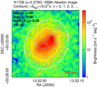
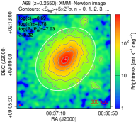
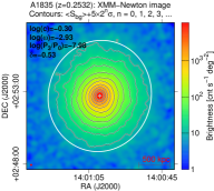
Figure 2: XMM-Newton images of A1758, A68 and A1835 after data processing. The image fluctuation $\sigma$ is calculated in a surrounding clean area after the mean brightness of background $\langle S_{\rm bg}\rangle$ is determined. The images are fitted with a model as indicated by the white ellipse at the level of $\langle S_{\rm bg}\rangle$+5$\sigma$, with the modeled cluster center indicated by the white cross. The smooth scale is indicated as the small red circle in the bottom-left corner, and the 500 kpc scale is plotted on the bottom-right corner.

Table 1: Dynamical parameters for 1308 clusters observed by the XMM-Newton (see http://zmtt.bao.ac.cn/galaxy_clusters/dyXimages/ for the full table).

Name	obsID	RA	DEC	$z$	${\rm log}_{10}(c)$	${\rm log}_{10}(\omega)$	${\rm log}_{10}(P_{3}/P_{0})$	$\kappa$	${\rm log}_{10}(\alpha)$	$\delta$	Notes
(1)	(2)	(3)	(4)	(5)	(6)	(7)	(8)	(9)	(10)	(11)	(12)
RXCJ0000.1+0816	0741581501	0.02958	8.27444	0.0396	-0.14$\pm$0.01	-4.04$\pm$0.08	-6.50$\pm$0.01	0.89	-2.46$\pm$0.01	-0.81$\pm$0.01	–
A2690	0125310101	0.09120	-25.13822	0.0840	-0.60$\pm$0.01	-1.86$\pm$0.02	-6.66$\pm$0.05	2.54	-1.33$\pm$0.01	1.16$\pm$0.01	–
XMMXCSJ0002-3556	0145020201	0.56708	-35.94272	0.7704	-0.64$\pm$0.03	-1.41$\pm$0.03	-5.81$\pm$0.11	2.45	-1.19$\pm$0.01	1.19$\pm$0.01	–
A2715	0655300101	0.68944	-34.67154	0.1160	-0.76$\pm$0.01	-1.52$\pm$0.01	-5.64$\pm$0.03	2.30	-0.55$\pm$0.01	1.51$\pm$0.01	–
A2697	0652010401	0.79826	-6.09169	0.2484	-0.66$\pm$0.02	-2.38$\pm$0.02	-6.67$\pm$0.13	1.11	-1.90$\pm$0.01	-0.27$\pm$0.01	–
A2717	0145020201	0.80042	-35.92722	0.0490	-0.39$\pm$0.01	-3.32$\pm$0.01	-7.54$\pm$0.05	1.03	-1.93$\pm$0.01	-0.35$\pm$0.01	c
A2700	0201900101	0.96083	2.06333	0.0924	-0.51$\pm$0.01	-3.05$\pm$0.03	-7.88$\pm$0.10	1.40	-2.29$\pm$0.01	-0.33$\pm$0.01	–
ZGXJ000402-355635	0145020201	1.00742	-35.94317	0.4974	-0.58$\pm$0.04	-2.12$\pm$0.05	-6.15$\pm$0.13	2.17	-1.42$\pm$0.01	0.83$\pm$0.01	–
WHLJ000524+161309	0783270101	1.35000	16.21917	0.1160	-0.73$\pm$0.01	-1.66$\pm$0.01	-6.62$\pm$0.03	2.05	-1.39$\pm$0.01	0.76$\pm$0.01	–
A2734	0675470801	2.83625	-28.85500	0.0625	-0.63$\pm$0.01	-2.66$\pm$0.03	-6.72$\pm$0.02	1.85	-1.37$\pm$0.01	0.62$\pm$0.01	c

Columns: (1) cluster name; (2) observation ID; (3-4) right ascension and declination in J2000; (5) redshift; (6) the concentration index; (7) the centroid shift; (8) the power ratio; (9) the profile parameter; (10) the asymmetry factor; (11) the morphology index; (12) Notes: “–” observed only by the XMM-Newton, “c” also observed by the Chandra.

2.2 X-ray image processing

The data of 1308 clusters of galaxies are processed in the XMM-Newton Science Analysis System (SAS, Gabriel et al., 2004, version: 18.0.0) with the latest Current Calibration Files (CCFs) synchronised to the CCF repository of the XMM-Newton. The Observation Data Files (ODFs) for all clusters are downloaded with the collected observation ID. The CCFs for a given cluster are selected from the repository with the command cifbuild, and the summary file for observation information is produced by running odfingest. To filter the effect of soft proton excesses, the event files are cleaned by emchain and mos-filter for the MOS systems, and by epchain and pn-filter for the PN system. To be consistent with data in Yuan & Han (2020), only photons in 0.5-5 keV are taken. After a series of routines (e.g., cheese, mos/pn-spectra, mos/pn-back, proton, …, see a thread as an example), we obtain the X-ray count image, the exposure image, the Quiescent Particle Background (QPB) image and the soft proton image for clusters. Images for MOS1, MOS2 and PN systems are merged with the routine comb. Then the background are subtracted and the exposure are corrected by the tool adapt. The Point Spread Function (PSF) for each cluster is generated with the SAS tool psfgen, that will be used to deconvolve the observed image.

To calculate the dynamical parameters, as done by Yuan & Han (2020), the point sources in the field must be discounted. The point sources are detected with the CIAO routine wavdetect, and the “holes” of subtracted images are filled with the tool dmfilth according to the ambient brightness (see the Section 2.2 in Yuan & Han, 2020, for details). To avoid possible biases caused by different physical scales indicated by the image pixel for clusters at different redshifts, the X-ray images of clusters are smoothed to a certain physical scale of 30 kpc with a circular Gaussian model. For few clusters with very low redshift $z<0.03$ the images are smoothed to 10 kpc. For 7 clusters without available redshifts, the images are smoothed to 5 arcseconds. The processed X-ray images for all clusters are available on the web-page: http://zmtt.bao.ac.cn/galaxy_clusters/dyXimages/, and three examples are given in Fig. 2. The images for 22 clusters newly released by the Chandra are processed in the same way as Yuan & Han (2020).

After all images are processed, we get 351 clusters which are common in both the Chandra and XMM-Newton databases.

3 Parameters for dynamical states

The dynamical state of galaxy clusters can be quantitatively determined from their X-ray images. In this section, we calculate three widely used parameters, i.e., the concentration index $c$, the centroid shift $\omega$ and the power ratio $P_{3}/P_{0}$, and also the morphology index $\delta$ defined in Yuan & Han (2020), which is derived in the elliptical regions adapting to the actual size and shape of clusters. Definitions for these dynamical parameters are as followings.

The concentration index $c$ is defined by Santos et al. (2008) as being

$$c=\frac{S_{\rm core}}{S_{\rm tot}}=\frac{\sum\limits_{R<\rm R_{\rm core}}f_{\rm obs}(x_{i},y_{i})}{\sum\limits_{R<\rm R_{ap}}f_{\rm obs}(x_{i},y_{i})},$$ (1)

where $f_{\rm obs}(x_{i},y_{i})$ is the brightness corresponding to the pixel $(x_{i},y_{i})$. Here the fluxes from the core and the whole regions of clusters, $S_{\rm core}$ and $S_{\rm tot}$, are integrations of X-ray images around the model-fitted center, i.e., the white crosses in Fig. 2, rather than around the brightness peak of images. To be consistent with previous works (e.g., Cassano et al., 2010, 2013; Yuan & Han, 2020), the core radius $R_{\rm core}$ and the radius for whole cluster $R_{\rm ap}$ are set as 100 kpc and 500 kpc, respectively. For relaxed clusters with a very bright core, the gas is gradually sink to the center, so that the concentration index $c$ should approach towards 1.0. For merging clusters with disturbed structures, the $c$ could be very small. Because of the large PSF of the XMM-Newton ($\sim$5” for EPIC-PN and $\sim$6” for EPIC-MOS, corresponding to $\sim$20 kpc if $z=0.2$), the cluster center and the concentration index are determined from PSF-deconvolved X-ray images (e.g., Lovisari et al., 2017).

For merging clusters, large offsets appear between the brightness peak and the centroid, i.e. the fitted cluster center (e.g., Kolokotronis et al., 2001; Zenteno et al., 2020). Based on the simulations by Poole et al. (2006), Cassano et al. (2010) clearly wrote the formula as being

$$\omega=[\frac{1}{n-1}\sum\limits_{i}(\Delta_{i}-\langle\Delta\rangle)^{2}]^{\frac{1}{2}}\times\frac{1}{R_{\rm ap}}.$$ (2)

Within the aperture radius of $R_{\rm ap}=500$kpc, the centroid can be found in a series of circular apertures with a decreasing step of 5%, so that a series of offsets can be obtained. The standard deviation of these offsets from all $i$th apertures are calculated and normalized to $R_{\rm ap}$, which is defined as $\omega$. A small $\omega$ implies a relaxed cluster.

Cluster mergers often trigger substructures and fluctuations in the X-ray images (see pictures in Mann & Ebeling, 2012). Buote & Tsai (1995) characterized substructures of clusters in various scales and defined the ratio between $P_{3}$ and $P_{0}$ as a good dynamical proxy. The $P_{m}$ is calculated as being

$$\begin{split}&P_{0}=[a_{0}\ln(R_{\rm ap})]^{2},\\ &P_{m}=\frac{1}{2m^{2}R_{\rm ap}^{2m}}(a_{m}^{2}+b_{m}^{2}).\end{split}$$ (3)

Often used is $m=3$ for $P_{3}$. The $a_{m}$ and $b_{m}$ is obtained through

$$\begin{split}a_{m}=\int_{r\leq R_{\rm ap}}f_{\rm obs}(x_{i},y_{i})(r)^{m}\cos(m\phi)dx_{i}dy_{i},\\ b_{m}=\int_{r\leq R_{\rm ap}}f_{\rm obs}(x_{i},y_{i})(r)^{m}\sin(m\phi)dx_{i}dy_{i},\end{split}$$ (4)

where $r$ is the distance of a pixel $(x_{i},y_{i})$ to the cluster center, $\phi$ is the position angle of the pixel $(x_{i},y_{i})$.

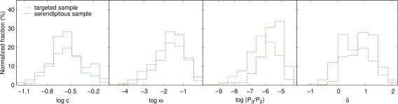
Figure 3: Distribution of dynamical parameters for clusters in the targeted sample (solid) and the serendipitous sample (dashed).

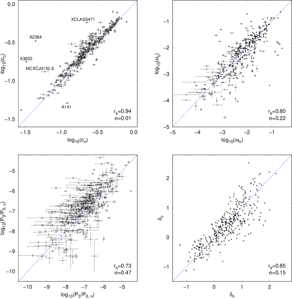
Figure 4: Comparison between the concentration indexes (upper-left), centroid shifts (upper-right), power ratios (lower-left) and morphology indexes (lower-right) for 351 clusters derived from XMM-Newton (X-axis, with a subscript “n”) and derived from Chandra images (Y-axis, with a subscript “c” ). The dotted line in each panel indicates equivalent values in X and Y axes. The name of 5 outliers are labeled in the top-left panel. The Spearman rank-order correlation coefficient $r_{\rm s}$ and the intrinsic scatter $\sigma$ are marked in each panel.

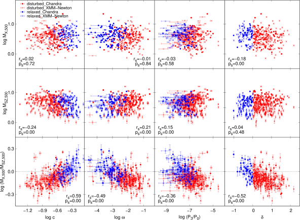
Figure 5: Dependence of mass estimation on the dynamical parameters. Top panels are for $M_{\rm X,500}$ (taken from Piffaretti et al., 2011), middle panels for $M_{\rm SZ,500}$ (taken from Planck Collaboration et al., 2016), and bottom panels for the deviations of the mass estimation expressed by the mass ratio in logarithm. Dynamical parameters of clusters are taken from Table 4. Dynamical parameters derived from XMM-Newton images are marked as crosses, while those from Chandra images are presented as dots. Clusters with $\delta\geq 0$ are regarded as disturbed clusters (red), while those with $\delta<0$ are classified as relaxed clusters (blue). The correlation coefficient $r_{\rm s}$ and relevant significance $p_{\rm s}$ are labelled in each panel.

Note that the concentration index, the centroid shift and the power ratio are all calculated in a circular region with a given radius of $R_{\rm ap}=500$ kpc, so that the distance or redshift of a cluster is desired for such calculations. In principle, one can use the mass-related radius $R_{500}$ for calculation within which the mean density of material is 500 times of the critical density of the Universe at the cluster redshift. Yuan & Han (2020) found that the values of concentration indexes, centroid shifts and power ratios derived in 500 kpc are well correlated with those from literature calculated in $R_{500}$ or a fraction of it (e.g., Weißmann et al., 2013a, b; Donahue et al., 2016; Andrade-Santos et al., 2017). As discussed in Yuan & Han (2020), we do not use it for calculations with following reasons. (1) The $R_{500}$ has to be derived during the process of mass estimation, so that the observation must have sufficient X-ray photons to derive the radial profiles of temperature and electron density, which may not be possible for many clusters. (2) The typical size of $R_{500}$ is about 1 Mpc (e.g., Piffaretti et al., 2011), leading a deficient CCD coverage for clusters with $z<0.1$ (over 400 clusters, see Fig. 1). (3) The $R_{500}$ is derived under the assumptions of spherical symmetry and virial equilibrium for clusters. Our motivation is deriving dynamical parameters for clusters as many as possible, here we simply take $R_{\rm ap}=500$ kpc for calculations.

Considering the actual size and shape of clusters, Yuan & Han (2020) defined a morphology index $\delta$, which is adoptive to any cluster regardless the redshift is available or not and what shape it has (i.e. not necessary circular). First the brightness profile of clusters is fitted with an elliptical $\beta$-model (Cavaliere & Fusco-Femiano, 1976):

$$f_{\rm mod}(x_{i},y_{i})=f_{\rm mod}(r)=A(1+(\frac{r}{r_{0}})^{2})^{-\beta}+C,$$ (5)

where

$$r(x_{i},y_{i})=\frac{\sqrt{x^{2}(1-\epsilon)^{2}+y^{2}}}{1-\epsilon},$$ (6)

and

$$\begin{split}x=(x_{i}-x_{0})\cos\theta+(y_{i}-y_{0})\sin\theta,\\ y=(y_{i}-y_{0})\cos\theta-(x_{i}-x_{0})\sin\theta.\end{split}$$ (7)

Here $(x_{0},y_{0})$, $A$, $r_{0}$ and $\beta$ are, respectively, the center, the maximum, the characteristic radius and the slope index of the best fitted model, $C$ stands for the average brightness of background, and $\epsilon$ and $\theta$ are the fitted ellipticity and the orientation angle. The profile parameter $\kappa$ is thus defined as

$$\kappa=\frac{1+\epsilon}{\beta}.$$ (8)

In the other hand, the asymmetry factor $\alpha$ can be calculated as being

$$\alpha=\frac{\sum\limits_{x_{i},y_{i}}{[f_{\rm obs}(x_{i},y_{i})-f_{\rm obs}(x_{i}^{\prime},y_{i}^{\prime})]^{2}}}{\sum\limits_{x_{i},y_{i}}{f^{2}_{\rm obs}(x_{i},y_{i})}}\times 100\;\%,$$ (9)

where $(x_{i},y_{i})$ and $(x_{i}^{\prime},y_{i}^{\prime})$ are the symmetric pixel pair to the center $(x_{0},y_{0})$. The morphology index $\delta$ finally defined as the combination of the profile parameter $\kappa$ and the asymmetry factor $\alpha$ as

$$\delta =0.68\rm{log_{10}}(\alpha)+0.73\kappa+0.21,$$ (10)

which can best separate the relaxed and disturbed clusters in the $\kappa-\alpha$ space (Yuan & Han, 2020).

We calculate the concentration index $c$, the centroid shift $\omega$ and the power ratio $P_{3}/P_{0}$ in a circular region for 1308 clusters found in the XMM-Newton archive, as listed in Table 1. The two morphology parameters $\kappa$ and $\alpha$, and the morphology index $\delta$ are calculated in an elliptical region with the size and shape adapting to the actual morphology of a cluster (see the white ellipses in Fig. 2).

Table 2: Dynamical parameters for 42 clusters in Yuan & Han (2020) with newly available redshifts and 22 clusters in the newly released Chandra data.

Name	obsID	RA	DEC	$z$	${\rm log}_{10}(c)$	${\rm log}_{10}(\omega)$	${\rm log}_{10}(P_{3}/P_{0})$	$\kappa$	${\rm log}_{10}(\alpha)$	$\delta$	Notes
(1)	(2)	(3)	(4)	(5)	(6)	(7)	(8)	(9)	(10)	(11)	(12)
SPTCLJ0013-4906	13462	3.33083	-49.11611	0.4075	-0.72$\pm$0.01	-1.50$\pm$0.01	-5.81$\pm$0.02	2.03	-0.48$\pm$0.01	1.37$\pm$0.01	1
SPTCLJ0033-6326	13483	8.46875	-63.44389	0.5963	-0.56$\pm$0.01	-2.04$\pm$0.02	-6.05$\pm$0.07	1.13	-0.98$\pm$0.01	0.37$\pm$0.01	1
SPTCLJ0058-6145	13479	14.58583	-61.76805	0.8300	-0.74$\pm$0.01	-2.20$\pm$0.01	-5.26$\pm$0.04	2.27	-0.84$\pm$0.01	1.30$\pm$0.01	1
SPTCLJ0102-4603	13485	15.67708	-46.07195	0.8405	-0.82$\pm$0.01	-1.35$\pm$0.01	-5.56$\pm$0.11	2.14	-0.50$\pm$0.01	1.43$\pm$0.01	1
SPTCLJ0123-4821	13491	20.79583	-48.35806	0.6550	-0.79$\pm$0.02	-1.82$\pm$0.01	-6.13$\pm$0.10	1.74	-0.92$\pm$0.01	0.86$\pm$0.01	1
RXCJ0138.0-2155	17186	24.51583	-21.92528	0.3380	-0.29$\pm$0.01	-3.51$\pm$0.01	-7.91$\pm$0.15	0.65	-1.63$\pm$0.01	-0.42$\pm$0.01	1
SPTCLJ0142-5032	13467	25.54583	-50.54000	0.6793	-0.80$\pm$0.05	-2.01$\pm$0.06	-5.94$\pm$0.17	2.28	-0.70$\pm$0.01	1.39$\pm$0.01	1
SPTCLJ0151-5954	13480	27.85708	-59.90805	1.0300	-0.86$\pm$0.01	-1.03$\pm$0.01	-6.57$\pm$0.16	2.86	-0.31$\pm$0.01	2.09$\pm$0.01	1
SPTCLJ0156-5541	13489	29.04208	-55.69806	1.2200	-0.63$\pm$0.01	-1.72$\pm$0.02	-7.92$\pm$0.55	1.46	-1.01$\pm$0.01	0.59$\pm$0.01	1
SPTCLJ0212-4656	13464	33.10792	-46.95000	0.6535	-0.90$\pm$0.01	-1.02$\pm$0.02	-5.32$\pm$0.04	2.51	-0.21$\pm$0.01	1.90$\pm$0.01	1
XCLASS1385	20783	35.78400	86.33700	0.1860	-0.52$\pm$0.01	-2.18$\pm$0.01	-5.04$\pm$0.01	2.16	-0.59$\pm$0.01	1.39$\pm$0.01	2
RXJ0236.0-5224	12096	39.02083	-52.41889	0.5900	-0.48$\pm$0.01	-1.93$\pm$0.02	-5.23$\pm$0.11	0.73	-0.75$\pm$0.01	0.23$\pm$0.01	1
SPTCLJ0252-4824	13494	43.21208	-48.41500	0.4207	-0.92$\pm$0.01	-1.11$\pm$0.01	-6.33$\pm$0.06	1.45	-0.71$\pm$0.01	0.78$\pm$0.01	1
SPTCLJ0307-5042	13476	46.96083	-50.70500	0.5500	-0.70$\pm$0.01	-2.76$\pm$0.02	-7.01$\pm$0.09	1.76	-0.99$\pm$0.01	0.82$\pm$0.01	1
CXO031027-203537	14236	47.61500	-20.59306	0.6916	-0.47$\pm$0.01	-2.17$\pm$0.01	-5.97$\pm$0.03	0.97	-1.38$\pm$0.01	-0.02$\pm$0.01	1
SPTCLJ0329-2330	18282	52.31750	-23.50306	1.2270	-0.72$\pm$0.01	-1.97$\pm$0.03	-6.47$\pm$0.06	1.69	-1.07$\pm$0.01	0.72$\pm$0.01	1
SPTCLJ0334-4659	13470	53.54708	-46.99611	0.4861	-0.44$\pm$0.01	-2.56$\pm$0.01	-6.86$\pm$0.07	1.13	-1.39$\pm$0.01	0.08$\pm$0.01	1
1WGAJ0337.8-2304	7991	54.46042	-23.07278	0.6200	-0.43$\pm$0.02	-2.16$\pm$0.02	-5.84$\pm$0.12	1.50	-1.31$\pm$0.01	0.42$\pm$0.01	1
PSZG208.57-44.31	18773	60.64958	-15.67500	0.8500	-0.56$\pm$0.01	-1.04$\pm$0.01	-3.55$\pm$0.03	2.58	-1.37$\pm$0.01	1.16$\pm$0.01	1
SPTCLJ0406-4804	13477	61.73083	-48.08194	0.7355	-0.64$\pm$0.01	-2.09$\pm$0.02	-5.31$\pm$0.05	2.04	-0.55$\pm$0.01	1.33$\pm$0.01	1
PSZ1G141.73+14.22	18289	70.25708	68.23528	0.8330	-0.62$\pm$0.03	-1.79$\pm$0.03	-7.95$\pm$0.55	1.72	-0.78$\pm$0.01	0.93$\pm$0.01	1
SPTCLJ0441-4854	13475	70.45084	-48.92389	0.8100	-0.49$\pm$0.02	-2.39$\pm$0.02	-5.87$\pm$0.11	0.87	-0.97$\pm$0.01	0.19$\pm$0.01	1
3C129.1	19965	72.51458	45.02417	0.0210	0.00$\pm$0.00	0.00$\pm$0.00	0.00$\pm$0.00	1.87	-1.59$\pm$0.01	0.49$\pm$0.01	1
SPTCLJ0456-5116	13474	74.11792	-51.27806	0.5619	-0.71$\pm$0.01	-1.93$\pm$0.03	-5.99$\pm$0.03	1.11	-0.92$\pm$0.01	0.40$\pm$0.01	1
PSZ1G127.02+26.21	18286	89.84666	86.22861	0.6300	-0.79$\pm$0.04	-1.41$\pm$0.19	-6.10$\pm$0.26	2.52	-0.50$\pm$0.01	1.71$\pm$0.01	1
PSZ1G224.01-11.14	18293	97.75291	-14.83500	0.6200	-0.77$\pm$0.01	-1.74$\pm$0.02	-6.78$\pm$0.18	1.91	-0.70$\pm$0.01	1.13$\pm$0.01	1
SPTCLJ0655-5234	13486	103.97375	-52.56805	0.4724	-0.76$\pm$0.01	-1.29$\pm$0.01	-5.82$\pm$0.01	1.20	-0.98$\pm$0.01	0.42$\pm$0.01	1
PSZ2G181.06+48.47	22650	144.85745	40.75748	0.2350	-0.99$\pm$0.01	-1.10$\pm$0.01	-5.49$\pm$0.01	2.13	-0.72$\pm$0.01	1.28$\pm$0.01	2
A1156	21709	166.23167	47.42083	0.2152	-0.79$\pm$0.01	-2.40$\pm$0.01	-8.53$\pm$0.49	1.73	-0.48$\pm$0.01	1.14$\pm$0.01	2
SDSSJ1142.8+1527	18277	175.69041	15.45778	1.1200	-0.52$\pm$0.02	-2.44$\pm$0.10	-6.23$\pm$0.12	2.18	-0.58$\pm$0.01	1.40$\pm$0.01	1
PSZ1G135.24+65.43	21715	184.77721	50.91310	0.5271	-0.97$\pm$0.02	-1.01$\pm$0.01	-5.83$\pm$0.20	1.75	-0.46$\pm$0.01	1.18$\pm$0.01	2
SPTCLJ1315-2806	23214	198.81100	-28.10910	1.3900	-0.45$\pm$0.01	-2.41$\pm$0.02	-5.14$\pm$0.05	1.24	-0.88$\pm$0.01	0.52$\pm$0.01	2
WHLJ132419.7+041907	23068	201.08197	4.31863	0.2615	-0.26$\pm$0.01	-3.27$\pm$0.01	-8.84$\pm$0.12	0.75	-2.03$\pm$0.01	-0.62$\pm$0.01	2
WHLJ133029.5+490848	21708	202.62276	49.14661	0.3353	-0.93$\pm$0.01	-1.29$\pm$0.01	-6.26$\pm$0.14	2.83	-0.48$\pm$0.01	1.95$\pm$0.01	2
SPTCLJ1342-2442	21567	205.50349	-24.70510	0.8100	-0.56$\pm$0.01	-1.52$\pm$0.01	-5.53$\pm$0.03	1.38	-0.71$\pm$0.01	0.74$\pm$0.01	2
WHLJ134737.4+501109	21714	206.90582	50.18583	0.2810	-0.31$\pm$0.01	-3.00$\pm$0.06	-6.93$\pm$0.05	0.85	-1.18$\pm$0.01	0.03$\pm$0.01	2
A1904	21712	215.53278	48.55620	0.0708	-0.89$\pm$0.01	-1.04$\pm$0.01	-5.57$\pm$0.01	2.30	-0.53$\pm$0.01	1.52$\pm$0.01	2
PSZ2G104.74+40.42	22641	236.59300	69.95050	0.6900	-1.07$\pm$0.03	-0.84$\pm$0.06	-5.79$\pm$0.43	1.45	-0.26$\pm$0.01	1.09$\pm$0.01	2
CIZAJ1809.0-0414	25087	272.25500	-4.24389	0.3050	-0.54$\pm$0.01	-3.07$\pm$0.02	-7.64$\pm$0.08	0.94	-1.77$\pm$0.01	-0.31$\pm$0.01	2
PSZ2G075.85+15.53	21544	287.78854	44.91729	—	—	—	—	0.81	-0.87$\pm$0.01	0.21$\pm$0.01	2
A3674	23363	305.20792	-30.03361	0.2073	-0.48$\pm$0.01	-2.01$\pm$0.01	-5.73$\pm$0.02	1.22	-1.16$\pm$0.01	0.31$\pm$0.01	2
SPTCLJ2215-3537	24614	333.76651	-35.62080	1.1600	-0.26$\pm$0.01	-2.59$\pm$0.01	-6.65$\pm$0.06	0.67	-0.89$\pm$0.01	0.10$\pm$0.01	2
SPTCLJ2218-4519	13501	334.74582	-45.31611	0.6365	-0.76$\pm$0.01	-1.68$\pm$0.01	-5.92$\pm$0.04	1.68	-0.86$\pm$0.01	0.85$\pm$0.01	1
PSZ1G048.22-51.60	18283	335.05209	-12.21639	0.5440	-0.72$\pm$0.01	-1.73$\pm$0.01	-6.21$\pm$0.05	1.49	-1.01$\pm$0.01	0.61$\pm$0.01	1
SPTCLJ2222-4834	13497	335.71210	-48.57695	0.6519	-0.51$\pm$0.01	-2.92$\pm$0.02	-6.39$\pm$0.04	1.45	-1.22$\pm$0.01	0.44$\pm$0.01	1
SPTCLJ2232-6000	13502	338.14084	-59.99805	0.5948	-0.41$\pm$0.01	-2.89$\pm$0.01	-6.58$\pm$0.03	0.99	-1.39$\pm$0.01	-0.01$\pm$0.01	1
SPTCLJ2233-5339	13504	338.31876	-53.65389	0.4396	-0.64$\pm$0.02	-1.57$\pm$0.02	-6.64$\pm$0.16	1.10	-1.11$\pm$0.01	0.26$\pm$0.01	1
SPTCLJ2236-4555	13507	339.21875	-45.93000	1.1600	-0.48$\pm$0.01	-2.22$\pm$0.01	-5.31$\pm$0.07	1.41	-0.53$\pm$0.01	0.88$\pm$0.01	1
SPTCLJ2245-6207	13499	341.26001	-62.11611	0.5800	-1.11$\pm$0.01	-1.74$\pm$0.02	-5.38$\pm$0.12	2.84	-0.22$\pm$0.01	2.13$\pm$0.01	1
SPTCLJ2258-4044	13495	344.70584	-40.74000	0.8971	-0.77$\pm$0.01	-1.92$\pm$0.01	-6.01$\pm$0.15	1.92	-0.64$\pm$0.01	1.17$\pm$0.01	1
SPTCLJ2259-6057	13498	344.75208	-60.96000	0.7500	-0.51$\pm$0.01	-2.43$\pm$0.01	-6.16$\pm$0.04	0.99	-1.13$\pm$0.01	0.16$\pm$0.01	1
SPTCLJ2301-4023	13505	345.47083	-40.38889	0.8349	-0.41$\pm$0.01	-1.83$\pm$0.05	-6.00$\pm$0.05	1.07	-0.91$\pm$0.01	0.38$\pm$0.01	1
SPTCLJ2306-5120	21549	346.61209	-51.33700	1.2700	-0.60$\pm$0.01	-1.62$\pm$0.02	-4.51$\pm$0.04	1.89	-0.79$\pm$0.01	1.05$\pm$0.01	2
SPTCLJ2315-2127	21571	348.82800	-21.45700	0.5400	-0.66$\pm$0.01	-2.45$\pm$0.03	-5.62$\pm$0.04	1.52	-0.97$\pm$0.01	0.66$\pm$0.01	2
SPTCLJ2317-3239	22654	349.45499	-32.66560	1.0500	-0.36$\pm$0.01	-2.78$\pm$0.01	-7.10$\pm$0.09	0.90	-1.38$\pm$0.01	-0.07$\pm$0.01	2
SPTCLJ2320-5233	21552	350.12509	-52.56410	0.7550	-0.48$\pm$0.04	-2.48$\pm$0.22	-3.39$\pm$1.28	2.24	-0.54$\pm$0.01	1.48$\pm$0.01	2
PSZ1G108.18-11.53	17213	350.62375	48.77500	0.3347	-1.05$\pm$0.01	-1.52$\pm$0.01	-5.52$\pm$0.13	2.69	-0.64$\pm$0.01	1.74$\pm$0.01	1
SPTCLJ2331-5736	22073	352.91891	-57.61550	1.3800	-1.01$\pm$0.02	-0.26$\pm$0.19	-6.28$\pm$0.29	2.87	-0.08$\pm$0.01	2.25$\pm$0.01	1
SPTCLJ2334-5308	21705	353.51501	-53.14100	1.2000	-0.39$\pm$0.03	-2.49$\pm$0.05	-3.98$\pm$0.07	1.07	-0.78$\pm$0.01	0.46$\pm$0.01	2
SPTCLJ2335-5434	23027	353.88101	-54.58600	0.8660	-0.32$\pm$0.01	-2.98$\pm$0.09	-4.39$\pm$0.06	1.00	-0.90$\pm$0.01	0.33$\pm$0.01	2
SPTCLJ2336-5252	23127	354.08771	-52.87250	1.2200	-0.43$\pm$0.02	-2.08$\pm$0.08	-3.34$\pm$0.03	1.38	-0.61$\pm$0.01	0.80$\pm$0.01	2
SPTCLJ2345-6406	13500	356.25000	-64.09889	0.9400	-0.79$\pm$0.01	-1.16$\pm$0.01	-5.53$\pm$0.02	1.42	-0.75$\pm$0.01	0.74$\pm$0.01	1
SPTCLJ2352-4657	13506	358.06790	-46.96000	0.7300	-0.66$\pm$0.01	-2.78$\pm$0.01	-5.68$\pm$0.05	2.10	-0.94$\pm$0.01	1.10$\pm$0.01	1
CODEX-59603	18636	359.43332	0.80194	0.0616	—	—	—	0.59	-1.69$\pm$0.01	-0.51$\pm$0.01	1

Columns: (1)-(11) same as in Table 1; (12) Notes: “1” for 42 clusters with newly available redshifts; “2” for clusters in newly released data.

In addition to the 1308 clusters from the XMM-Newton archive, the newly available redshifts are found for 42 clusters in the Chandra sample in Yuan & Han (2020), and we update their dynamical parameters. We smooth their images to 30 kpc, and re-calculate the dynamical parameters for these clusters, as listed in Table 2. Moreover, 22 newly-archived clusters are found in the Chandra database, their dynamical parameters are also calculated accordingly and listed in Table 2.

We present in Fig. 3 the distribution of dynamical parameters for 1308 clusters in the XMM-Newton sample, and find a continuous distribution from the disturbed to relaxed clusters. In general, the clusters in the serendipitous sample have a slightly higher fraction of disturbed clusters. In Fig. 4, we compare the values of dynamical parameters calculated based on XMM-Newton images and those based on Chandra images for 351 clusters which appear in both samples. They are very consistent and the dynamical parameters concentrate around the equivalent lines. The Spearman rank-order correlation coefficient $r_{\rm s}$ (defined in Press et al., 1992, p. 640) indicates a great degree of correlation. The intrinsic scatter $\sigma$ is calculated for the intrinsic dispersion of the correlation with data uncertainties subtracted (see the appendix of Yuan et al., 2015, for calculation). One can see that the concentration indexes have the best correlation among the four dynamical parameters calculated from X-ray images of the two satellites, except for A2384, A3653 and MCXCJ0152.6-1358, because the cluster center is now re-defined at a position between subclusters rather than at one subcluster by Yuan & Han (2020). The large departure for XCLASS471 is mainly caused by the poor quality of image observed by the Chandra. Also a correction was made to A141 because the bright central part should be kept as the cluster core, but that was mistakenly subtracted as a point source in Yuan & Han (2020).

In Appendix, we compose the samples of clusters, including the 964 clusters in Yuan & Han (2020), 22 clusters newly archived by the Chandra, and 1308 clusters here from XMM-Newton data. The better estimated dynamical parameters are taken if a cluster is in both datasets, finally the unified estimates for dynamical parameters are listed for 1844 clusters in Table 4.

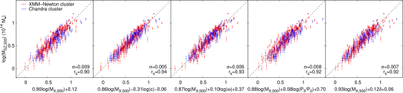
Figure 6: Including the dynamical parameters can improve the consistence between the mass estimations from the X-ray luminosity and the SZ effect. The mass data of 388 clusters are taken from Piffaretti et al. (2011) and Planck Collaboration et al. (2016), and the dynamical parameters from Table 4. The scaling relations thus can be improved as listed in Table 3.

Table 3: The scaling relations for mass estimations from X-ray data to that from the S-Z effect can be improved by considering dynamical state. The following formula are derived from 388 clusters.

Corrections to mass scales	$\sigma$	$r_{\rm s}$	$p_{\rm s}$
log${}_{10}(M_{\rm SZ,500})=0.90$log${}_{10}(M_{\rm X,500})+0.12$	0.009	0.90	0.00
log${}_{10}(M_{\rm SZ,500})=0.86$log${}_{10}(M_{\rm X,500})-0.31$log${}_{10}(c)-0.06$	0.005	0.94	0.00
log${}_{10}(M_{\rm SZ,500})=0.87$log${}_{10}(M_{\rm X,500})+0.10$log${}_{10}(\omega)+0.37$	0.006	0.93	0.00
log${}_{10}(M_{\rm SZ,500})=0.88$log${}_{10}(M_{\rm X,500})+0.08$log${}_{10}(P_{3}/P_{0})+0.70$	0.008	0.92	0.00
log${}_{10}(M_{\rm SZ,500})=0.93$log${}_{10}(M_{\rm X,500})+0.12\delta+0.06$	0.007	0.92	0.00

4 Influences of dynamical state on cluster mass estimations

Estimating masses of galaxy clusters is a key to various studies, such as the constraint of the cosmology parameters by using clusters (e.g., Vikhlinin et al., 2009; Böhringer et al., 2014). For this purpose the radial profiles of gas density and temperature of galaxy clusters should be derived first from X-ray images for a large sample of clusters. The total masses of clusters have been related to various observables, such as X-ray luminosities $L_{\rm X}$, gas temperatures $T$, intracluster gas masses $M_{\rm g}$, and the total energy of the ICM calculated through the SZ effect $Y_{\rm SZ}$ (e.g., Arnaud et al., 2005, 2007; Maughan, 2007; Morandi et al., 2007; Zhang et al., 2007; Zhang et al., 2008; Arnaud et al., 2010; Mantz et al., 2010; Reichert et al., 2011; Planck Collaboration et al., 2013). The scaling relations between masses and mass proxies are slightly shifted for subsamples of cool-core clusters and non-cool-core clusters (e.g., Chen et al., 2007; Zhao et al., 2013).

To verify the influences of dynamical state on cluster mass estimations, we take the masses $M_{\rm X,500}$ homogeneously derived by Piffaretti et al. (2011) for 1743 clusters mainly based on observations of ROSAT, and the masses estimated from SZ images $M_{\rm SZ,500}$ for 1653 clusters by Planck Collaboration et al. (2016). It has been widely accepted that cluster masses estimated from the integrated SZ signal are insensitive to the dynamical state of clusters (e.g., Motl et al., 2005; Bonaldi et al., 2007; Arnaud et al., 2010). Among these large samples, there are 388 clusters in our composite sample (Table 4) with dynamical parameters estimated. The X-ray and SZ mass estimates against dynamical parameters in the top and middle panels of Fig. 5 can be used to assess any dependence, the zero value of $p_{\rm s}$ indicates a robust correlation while none-zero value of $p_{\rm s}$ means no or fake correlation. A weak trend can be found for the $M_{\rm X,500}-\delta$, $M_{\rm SZ,500}-c$, $M_{\rm SZ,500}-\omega$ and $M_{\rm SZ,500}-P_{3}/P_{0}$ correlations, though the data scatter is rather large.

The deviation of mass estimates from the X-ray data, however, is clearly related to dynamical parameters. Because the X-ray mass $M_{\rm X,500}$ is mainly derived from thermal component of the ICM, while the SZ mass $M_{\rm SZ,500}$ is the integration of both the thermal and non-thermal parts. The dependence on dynamical parameters of mass estimate deviations indicate that the non-thermal energy in the ICM plays an important role in some disturbed clusters.

Any excellent scaling relation for mass estimation should diminish such a systematical deviation. If the SZ mass is taken as an ideal mass unaffected by the dynamical state of clusters, the scaling relations for the mass estimation from the X-ray measurements should include the small but systematical deviations caused by the dynamical state shown in the lowest panels of Fig. 5. As shown in the most left panel of Fig. 6 and also parameters in Table 3, the data scatter (i.e. the standard deviation $\sigma$) is the largest around the best fitted scaling line. However, when the dynamical parameters are included as the second term in the Table 3, the scatters in the other panels of Fig. 5 become smaller, especially for those data with large-deviations. The correlation parameter $r_{\rm s}$ in these plots is also improved (closer to 1.0), as listed in Table 3, though by only a small amount because of smaller weighted contributions to the mass estimation from dynamical parameters than that from the X-ray measurements themselves.

5 Summary

Dynamical state can be revealed from X-ray images. Following Yuan & Han (2020), we derive dynamical parameters for clusters of galaxies archived by the XMM-Newton satellite. We got data for 892 clusters from targeted observations, and also found 416 clusters serendipitously observed. The XMM-Newton images for these 1308 clusters are processed with the same procedures. We smoothed the X-ray images to a given physical scale of 30 kpc to calculate the concentration index, the centroid shift, the power ratio. The morphology index are calculated according to image sizes and shapes for all these clusters.

In addition, we calculated the dynamical parameters for 42 clusters in the Chandra sample of Yuan & Han (2020) because of the newly available redshifts, and also for 22 clusters in the newly released Chandra data.

Based on the results for 351 clusters which appear in both the XMM-Newton sample and Chandra sample, we found that dynamical parameters derived from XMM-Newton images are well consistent with those calculated with Chandra images.

We found the influence of dynamical state on cluster mass estimation. The scaling relation for masses estimation from the X-ray can be improved by including the dynamical parameters.

Data availability

The data underlying this article, including the full Table 1 and Table 4, the X-ray images for all clusters and the code for calculations, are available on the web-page http://zmtt.bao.ac.cn/galaxy_clusters/dyXimages/.

Appendix A Dynamical parameters derived from X-ray images of Chandra and XMM-Newton

Table 4: Dynamical parameters for 1844 clusters of galaxies derived from Chandra and XMM-Newton images. The full table is available on http://zmtt.bao.ac.cn/galaxy_clusters/dyXimages/.

Name	obsID	RA	DEC	$z$	${\rm log}_{10}(c)$	${\rm log}_{10}(\omega)$	${\rm log}_{10}(P_{3}/P_{0})$	$\kappa$	${\rm log}_{10}(\alpha)$	$\delta$	Note
(1)	(2)	(3)	(4)	(5)	(6)	(7)	(8)	(9)	(10)	(11)	(12)
RXCJ0000.1+0816	0741581501	0.02958	8.27444	0.0396	-0.14$\pm$0.01	-4.04$\pm$0.08	-6.50$\pm$0.01	0.89	-2.46$\pm$0.01	-0.81$\pm$0.01	2
A2690	0125310101	0.09120	-25.13822	0.0840	-0.60$\pm$0.01	-1.86$\pm$0.02	-6.66$\pm$0.05	2.54	-1.33$\pm$0.01	1.16$\pm$0.01	2
SPTCLJ0000-5748	18238	0.25000	-57.80695	0.7020	-0.29$\pm$0.01	-3.50$\pm$0.01	-8.15$\pm$0.22	0.80	-1.19$\pm$0.01	-0.02$\pm$0.01	1
SPTCLJ0001-5440	19761	0.40583	-54.66972	0.7300	-0.50$\pm$0.01	-1.53$\pm$0.01	-3.99$\pm$0.05	1.40	-0.34$\pm$0.01	1.00$\pm$0.01	1
XMMXCSJ0002-3556	0145020201	0.56708	-35.94272	0.7704	-0.64$\pm$0.03	-1.41$\pm$0.03	-5.81$\pm$0.11	2.45	-1.19$\pm$0.01	1.19$\pm$0.01	2
A2715	0655300101	0.68944	-34.67154	0.1160	-0.76$\pm$0.01	-1.52$\pm$0.01	-5.64$\pm$0.03	2.30	-0.55$\pm$0.01	1.51$\pm$0.01	2
A2697	0652010401	0.79826	-6.09169	0.2484	-0.66$\pm$0.02	-2.38$\pm$0.02	-6.67$\pm$0.13	1.11	-1.90$\pm$0.01	-0.27$\pm$0.01	2
A2717	0145020201	0.80042	-35.92722	0.0490	-0.39$\pm$0.01	-3.32$\pm$0.01	-7.54$\pm$0.05	1.03	-1.93$\pm$0.01	-0.35$\pm$0.01	4
A2700	0201900101	0.96083	2.06333	0.0924	-0.51$\pm$0.01	-3.05$\pm$0.03	-7.88$\pm$0.10	1.40	-2.29$\pm$0.01	-0.33$\pm$0.01	2
ZGXJ000402-355635	0145020201	1.00742	-35.94317	0.4974	-0.58$\pm$0.04	-2.12$\pm$0.05	-6.15$\pm$0.13	2.17	-1.42$\pm$0.01	0.83$\pm$0.01	2

Columns: (1) cluster name; (2) observation ID; (3-4) right ascension and declination in J2000; (5) redshift; (6) the concentration index; (7) the centroid shift; (8) the power ratio; (9) the profile parameter; (10) the asymmetry factor; (11) the morphology index; (12) Note: “1” cluster only observed by Chandra; “2” only observed by XMM-Newton; “3” cluster with both Chandra and XMM-Newton images, parameters derived from Chandra images are taken; “4” cluster with both but parameters from XMM-Newton; “5” cluster from newly released archive of Chandra, “6” clusters from Chandra with newly available redshift.

To ease the usage of dynamical parameters for 964 clusters in Yuan & Han (2020), for 64 clusters updated in this paper with Chandra images, and for 1308 clusters with XMM-Newton images, we make an uniform list for 1844 clusters, as presented in Table 4. For clusters with both Chandra and XMM-Newton observations, we choose the one with better quality of imaging, such as higher signal-to-noise ratio (e.g., MCXCJ0152.6-1358 and PSZ2G243.15-73.84) or better CCD coverage (e.g., A13 and A399).

References

- Abell et al. (1989) Abell G. O., Corwin Jr. H. G., Olowin R. P., 1989, ApJS, 70, 1
- Aguerri & Sánchez-Janssen (2010) Aguerri J. A. L., Sánchez-Janssen R., 2010, A&A, 521, A28
- Andrade-Santos et al. (2017) Andrade-Santos F., et al., 2017, ApJ, 843, 76
- Arnaud et al. (2005) Arnaud M., Pointecouteau E., Pratt G. W., 2005, A&A, 441, 893
- Arnaud et al. (2007) Arnaud M., Pointecouteau E., Pratt G. W., 2007, A&A, 474, L37
- Arnaud et al. (2010) Arnaud M., Pratt G. W., Piffaretti R., Böhringer H., Croston J. H., Pointecouteau E., 2010, A&A, 517, A92
- Bauer et al. (2005) Bauer F. E., Fabian A. C., Sanders J. S., Allen S. W., Johnstone R. M., 2005, MNRAS, 359, 1481
- Böhringer et al. (2014) Böhringer H., Chon G., Collins C. A., 2014, A&A, 570, A31
- Bonaldi et al. (2007) Bonaldi A., Tormen G., Dolag K., Moscardini L., 2007, MNRAS, 378, 1248
- Buote & Tsai (1995) Buote D. A., Tsai J. C., 1995, ApJ, 452, 522
- Cassano et al. (2010) Cassano R., Ettori S., Giacintucci S., Brunetti G., Markevitch M., Venturi T., Gitti M., 2010, ApJ, 721, L82
- Cassano et al. (2013) Cassano R., et al., 2013, ApJ, 777, 141
- Cavaliere & Fusco-Femiano (1976) Cavaliere A., Fusco-Femiano R., 1976, A&A, 49, 137
- Chen et al. (2007) Chen Y., Reiprich T. H., Böhringer H., Ikebe Y., Zhang Y.-Y., 2007, A&A, 466, 805
- Chon & Böhringer (2017) Chon G., Böhringer H., 2017, A&A, 606, L4
- Cialone et al. (2018) Cialone G., De Petris M., Sembolini F., Yepes G., Baldi A. S., Rasia E., 2018, MNRAS, 477, 139
- Colless & Dunn (1996) Colless M., Dunn A. M., 1996, ApJ, 458, 435
- Cuciti et al. (2015) Cuciti V., Cassano R., Brunetti G., Dallacasa D., Kale R., Ettori S., Venturi T., 2015, A&A, 580, A97
- Donahue et al. (2016) Donahue M., et al., 2016, ApJ, 819, 36
- Dressler & Shectman (1988) Dressler A., Shectman S. A., 1988, AJ, 95, 985
- Einasto et al. (2010) Einasto M., et al., 2010, A&A, 522, A92
- Einasto et al. (2012) Einasto M., et al., 2012, A&A, 540, A123
- Flin & Krywult (2006) Flin P., Krywult J., 2006, A&A, 450, 9
- Gabriel et al. (2004) Gabriel C., et al., 2004, in Ochsenbein F., Allen M. G., Egret D., eds, Astronomical Society of the Pacific Conference Series Vol. 314, Astronomical Data Analysis Software and Systems (ADASS) XIII. p. 759
- Geller & Beers (1982) Geller M. J., Beers T. C., 1982, PASP, 94, 421
- Halliday et al. (2004) Halliday C., et al., 2004, A&A, 427, 397
- Hou et al. (2009) Hou A., Parker L. C., Harris W. E., Wilman D. J., 2009, ApJ, 702, 1199
- Klein et al. (2019) Klein M., et al., 2019, Monthly Notices of the Royal Astronomical Society, 488, 739
- Kolokotronis et al. (2001) Kolokotronis V., Basilakos S., Plionis M., Georgantopoulos I., 2001, MNRAS, 320, 49
- Koulouridis et al. (2021) Koulouridis E., et al., 2021, A&A, 652, A12
- Liu et al. (2018) Liu A., Tozzi P., Yu H., De Grandi S., Ettori S., 2018, MNRAS,
- Lopes et al. (2018) Lopes P. A. A., Trevisan M., Laganá T. F., Durret F., Ribeiro A. L. B., Rembold S. B., 2018, MNRAS, 478, 5473
- Lovisari et al. (2017) Lovisari L., et al., 2017, ApJ, 846, 51
- Mann & Ebeling (2012) Mann A. W., Ebeling H., 2012, MNRAS, 420, 2120
- Mantz et al. (2010) Mantz A., Allen S. W., Ebeling H., Rapetti D., Drlica-Wagner A., 2010, MNRAS, 406, 1773
- Maughan (2007) Maughan B. J., 2007, ApJ, 668, 772
- Morandi et al. (2007) Morandi A., Ettori S., Moscardini L., 2007, MNRAS, 379, 518
- Motl et al. (2005) Motl P. M., Hallman E. J., Burns J. O., Norman M. L., 2005, ApJ, 623, L63
- Piffaretti et al. (2011) Piffaretti R., Arnaud M., Pratt G. W., Pointecouteau E., Melin J.-B., 2011, A&A, 534, A109
- Planck Collaboration et al. (2013) Planck Collaboration et al., 2013, A&A, 550, A129
- Planck Collaboration et al. (2016) Planck Collaboration et al., 2016, A&A, 594, A27
- Poole et al. (2006) Poole G. B., Fardal M. A., Babul A., McCarthy I. G., Quinn T., Wadsley J., 2006, MNRAS, 373, 881
- Press et al. (1992) Press W. H., Teukolsky S. A., Vetterling W. T., Flannery B. P., 1992, Numerical recipes in FORTRAN. The art of scientific computing
- Ramella et al. (2007) Ramella M., et al., 2007, A&A, 470, 39
- Reichert et al. (2011) Reichert A., Böhringer H., Fassbender R., Mühlegger M., 2011, A&A, 535, A4
- Roberts et al. (2018) Roberts I. D., Parker L. C., Hlavacek-Larrondo J., 2018, MNRAS, 475, 4704
- Rykoff et al. (2014) Rykoff E. S., et al., 2014, ApJ, 785, 104
- Santos et al. (2008) Santos J. S., Rosati P., Tozzi P., Böhringer H., Ettori S., Bignamini A., 2008, A&A, 483, 35
- Solanes et al. (1999) Solanes J. M., Salvador-Solé E., González-Casado G., 1999, A&A, 343, 733
- Vikhlinin et al. (2009) Vikhlinin A., et al., 2009, ApJ, 692, 1060
- Weißmann et al. (2013a) Weißmann A., Böhringer H., Šuhada R., Ameglio S., 2013a, A&A, 549, A19
- Weißmann et al. (2013b) Weißmann A., Böhringer H., Chon G., 2013b, A&A, 555, A147
- Wen & Han (2013) Wen Z. L., Han J. L., 2013, MNRAS, 436, 275
- Wen & Han (2015) Wen Z. L., Han J. L., 2015, MNRAS, 448, 2
- Wen et al. (2012) Wen Z. L., Han J. L., Liu F. S., 2012, ApJS, 199, 34
- Wen et al. (2018) Wen Z. L., Han J. L., Yang F., 2018, MNRAS, 475, 343
- West & Bothun (1990) West M. J., Bothun G. D., 1990, ApJ, 350, 36
- Yahil & Vidal (1977) Yahil A., Vidal N. V., 1977, ApJ, 214, 347
- Yu et al. (2018) Yu H., Diaferio A., Serra A. L., Baldi M., 2018, ApJ, 860, 118
- Yuan & Han (2020) Yuan Z. S., Han J. L., 2020, MNRAS, 497, 5485
- Yuan et al. (2015) Yuan Z. S., Han J. L., Wen Z. L., 2015, ApJ, 813, 77
- Zenteno et al. (2020) Zenteno A., et al., 2020, MNRAS, 495, 705
- Zhang et al. (2007) Zhang Y.-Y., Finoguenov A., Böhringer H., Kneib J.-P., Smith G. P., Czoske O., Soucail G., 2007, A&A, 467, 437
- Zhang et al. (2008) Zhang Y.-Y., Finoguenov A., Böhringer H., Kneib J.-P., Smith G. P., Kneissl R., Okabe N., Dahle H., 2008, A&A, 482, 451
- Zhang et al. (2017) Zhang Y.-Y., et al., 2017, A&A, 599, A138
- Zhao et al. (2013) Zhao H.-H., Jia S.-M., Chen Y., Li C.-K., Song L.-M., Xie F., 2013, ApJ, 778, 124
- Zou et al. (2021) Zou H., et al., 2021, ApJS, 253, 56