Abstract

Contrastive learning is a highly effective method for learning representations from unlabeled data. Recent works show that contrastive representations can transfer across domains, leading to simple state-of-the-art algorithms for unsupervised domain adaptation. In particular, a linear classifier trained to separate the representations on the source domain can also predict classes on the target domain accurately, even though the representations of the two domains are far from each other. We refer to this phenomenon as linear transferability. This paper analyzes when and why contrastive representations exhibit linear transferability in a general unsupervised domain adaptation setting. We prove that linear transferability can occur when data from the same class in different domains (e.g., photo dogs and cartoon dogs) are more related with each other than data from different classes in different domains (e.g., photo dogs and cartoon cats) are. Our analyses are in a realistic regime where the source and target domains can have unbounded density ratios and be weakly related, and they have distant representations across domains.

1 Introduction

In recent years, contrastive learning and related ideas have been shown to be highly effective for representation learning (Chen et al., 2020a, b, He et al., 2020, Caron et al., 2020, Chen et al., 2020c, Gao et al., 2021, Su et al., 2021, Chen and He, 2020). Contrastive learning trains representations on unlabeled data by encouraging positive pairs (e.g., augmentations of the same image) to have closer representations than negative pairs (e.g., augmentations of two random images). The learned representations are almost linearly separable: one can train a linear classifier on top of the fixed representations and achieve strong performance on many natural downstream tasks (Chen et al., 2020a). Prior theoretical works analyze contrastive learning by proving that semantically similar datapoints (e.g., datapoints from the same class) are mapped to geometrically nearby representations (Arora et al., 2019, Tosh et al., 2020, 2021, HaoChen et al., 2021). In other words, representations form clusters in the Euclidean space that respect the semantic similarity; therefore, they are linearly separable for downstream tasks where datapoints in the same semantic cluster have the same label.

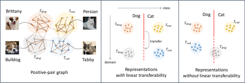
Figure 1: The linear transferability of representations. We demonstrate the linear transferability of representations when the unlabeled data contains images of two breeds of dogs (Brittanys, Bulldogs) and two breeds of cats (Persians, Tabbies). Left: A visualization of the positive-pair graph with four semantic clusters. Inter-cluster edges (dashed) have a much smaller weight than intra-cluster edges (solid). Inter-cluster edges between two breeds of dogs (or cats) have more weight than that between a dog cluster and a cat cluster. Middle and right: A visualization of two different types of representations: both have linear separability, but only the middle one has linear transferability. The red line is the decision boundary of a dog-vs-cat linear classifier trained in the representation space on labeled Brittanys ($S_{\text{dog}}$) vs. Persians ($S_{\text{cat}}$) images. The representation has linear transferability if this classifier is accurate on unlabeled Bulldogs ($T_{\text{dog}}$) vs. Tabbies ($T_{\text{cat}}$) images.

Intriguingly, recent empirical works show that contrastive representations carry richer information beyond the cluster memberships—they can transfer across domains in a linear way as elaborated below. Contrastive learning is used in many unsupervised domain adaptation algorithms(Thota and Leontidis, 2021, Sagawa et al., 2022) and the transferability leads to simple state-of-the-art algorithms (Shen et al., 2022, Park et al., 2020, Wang et al., 2021). In particular, Shen et al. (2022) observe that the relationship between two clusters can be captured by their relative positions in the representation space. For instance, as shown in Figure 1 (middle), suppose $S_{\text{dog}}$ and $S_{\text{cat}}$ are two classes in a source domain (e.g., Brittany dogs and Persian cats), and $T_{\text{dog}}$ and $T_{\text{cat}}$ are two classes in a target domain (e.g., Bulldogs and Tabby cats). A linear classifier trained to separate the representations of $S_{\text{dog}}$ and $S_{\text{cat}}$ turns out to classify $T_{\text{dog}}$ and $T_{\text{cat}}$ as well. This suggests the four clusters of representations are not located in the Euclidean space randomly (e.g., as in Figure 1 (right)), but rather in a more aligned position as in Figure 1 (middle). We refer to this phenomenon as the linear transferability of contrastive representations.

This paper analyzes when and why contrastive representations exhibit linear transferability in a general unsupervised domain adaptation setting. Evidently, linear transferability can only occur when clusters corresponding to the same class in two domains (e.g., Brittany dogs and Bulldogs) are somewhat related with each other. Somewhat surprisingly, we found that a weak relationship suffices: linear transferability occurs as long as corresponding classes in different domains are more related than different classes in different domains. Concretely, under this assumption (Assumptions 3.1 or 3.3), a linear head learned with labeled data on one domain (Algorithm 1) can successfully predict the classes on the other domain (Theorems 3.2 and 3.4). Notably, our analysis provably shows that representations from contrastive learning do not only encode cluster identities but also capture the inter-cluster relationship, hence explains the empirical success of contrastive learning for domain adaptation.

Compared to previous theoretical works on unsupervised domain adaptation (Shimodaira, 2000, Huang et al., 2006, Sugiyama et al., 2007, Gretton et al., 2008, Ben-David et al., 2010, Mansour et al., 2009, Kumar et al., 2020, Chen et al., 2020d, Cai et al., 2021), our results analyze a modern, practical algorithm with weaker and more realistic assumptions. We do not require bounded density ratios or overlap between the source and target domains, which were assumed in some classical works (Sugiyama et al., 2007, Ben-David et al., 2010, Zhang et al., 2019, Zhao et al., 2019). Another line of prior works (Kumar et al., 2020, Chen et al., 2020d) assume that data is Gaussian or near-Gaussian, whereas our result allows more general data distribution. Cai et al. (2021) analyze pseudolabeling algorithms for unsupervised domain adaptation, but require that the same-class cross-domain data are more related with each other (i.e., more likely to form positive pairs) than cross-class same-domain data are. We analyze a contrastive learning algorithm with strong empirical performance, and only require that the same-class cross-domain data are more related with each other than cross-class cross-domain data, which is intuitively and empirically more realistic as shown in Shen et al. (2022). (See related work and discussion below Assumption 3.1 for details).

Technically, we significantly extend the framework of HaoChen et al. (2021) to allow distribution shift—our setting only has labels on one subpopulation of the data (the source domain). Studying transferability to unlabeled subpopulations requires both novel assumptions (Assumptions 3.1 and 3.3) and novel analysis techniques (as discussed in Section 4).

Our analysis also introduces a variant of the linear probe—instead of training the linear head with the logistic loss, we learn it by directly computing the average representations within a class, multiplied by a preconditioner matrix (Algorithm 1). We empirically test this linear classifier on benchmark datasets and show that it achieves superior domain adaptation performance in Section 5.

Additional Related Works.

A number of papers have analyzed the linear separability of representations from contrastive learning (Arora et al., 2019, Tosh et al., 2020, 2021, HaoChen et al., 2021) and self-supervised learning (Lee et al., 2020), whereas we analyze the linear transferability.  Shen et al. (2022) also analyze the linear transferability but only for toy examples where the data is generated by a stochastic block model. Their technique requires a strong symmetry of the positive-pair graph (which likely does not hold in practice) so that top eigenvectors can be analytically derived. Our analysis is much more general and does not rely on explicit, clean form of the eigenvectors (which is impossible for general graphs).

Empirically, pre-training on a larger unlabeled dataset and then fine-tuning on a smaller labeled dataset is one of the most successful approaches for handling distribution shift (Blitzer et al., 2007, Ziser and Reichart, 2018, 2017, Ben-David et al., 2020, Chen et al., 2012, Xie et al., 2020, Jean et al., 2016, Hendrycks et al., 2020, Kim et al., 2022, Kumar et al., 2022, Sagawa et al., 2022, Thota and Leontidis, 2021, Shen et al., 2022). Recent advances in the scale of unlabeled data, such as in BERT and CLIP, have increased the importance of this approach (Wortsman et al., 2022, 2021). Despite the empirical progress, there has been limited theoretical understanding of why pre-training helps domain shift. Our work provides the first analysis that shows pre-trained representations with a supervised linear head trained on one domain can provably generalize to another domain.

2 Preliminaries

In this section, we introduce the contrastive loss, define the positive-pair graph, and introduce the basic assumptions on the clustering structure in the positive-pair graph.

Positive pairs.

Contrastive learning algorithms rely on the notion of “positive pairs”, which are pairs of semantically similar/related data. Let $\mathcal{X}$ be the set of population data and $P_{+}$ be the distribution of positive pairs of data satisfying $P_{+}(x,x^{\prime})=P_{+}(x^{\prime},x)$ for any $x,x^{\prime}\in\mathcal{X}$. We note that though a positive pair typically consists of semantically related data, the vast majority of semantically related pairs are not positive pairs. In the context of computer vision problems (Chen et al., 2020a), these pairs are usually generated via data augmentation on the same image.

For the ease of exposition, we assume $\mathcal{X}$ is a finite but large set (e.g., all real vectors in $\mathbb{R}^{d}$ with bounded precision) of size $N$. We use $P_{\mathcal{X}}$ to denote the marginal distribution of $P_{+}$, i.e., $P_{\mathcal{X}}(x):=\sum_{x^{\prime}\in\mathcal{X}}P_{+}(x,x^{\prime})$. Following the terminology in the literature (Arora et al., 2019), we call $(x,x^{\prime})$ a “negative pair” if $x$ and $x^{\prime}$ are independent random samples from $P_{\mathcal{X}}$.

Generalized spectral contrastive loss.

Contrastive learning trains a representation function (feature extractor) by minimizing a certain form of contrastive loss. Formally, let $f:\mathcal{X}\rightarrow\mathbb{R}^{k}$ be a mapping from data to $k$-dimensional features. In this paper, we consider a more general version of the spectral contrastive loss proposed in HaoChen et al. (2021). Let $I_{k\times k}$ be the $k$-dimensional identity matrix. We consider the following loss with regularization strength $\sigma>0$:

$$\mathcal{L}_{\sigma}(f)=\underset{(x,x^{+})\sim P_{+}}{\mathrm{\mathbb{E}}}\big{[}\left\lVert f(x)-f(x^{+})\right\rVert_{2}^{2}\big{]}+\sigma\cdot R(f),$$ (1)

where the regularizer is defined as

$$R(f)=\Big{\|}\underset{x\sim P_{\mathcal{X}}}{\mathrm{\mathbb{E}}}\big{[}f(x)f(x)^{\top}\big{]}-I_{k\times k}\Big{\|}_{F}^{2}.$$ (2)

The loss $\mathcal{L}_{\sigma}$ intuitively minimizes the closeness of positive pairs via its first term, while regularizing the representations’ covariance to be identity, avoiding all the representations to collapse to the same point. Simple algebra shows that $\mathcal{L}_{\sigma}$ recovers the original spectral contrastive loss when $\sigma=1$ (see Proposition B.1 for a formal derivation). We note that this loss is similar in spirit to the recently proposed Barlow Twins loss (Zbontar et al., 2021).

The positive-pair graph.

One useful way to think of positive pairs is through a graph defined by their distribution. Let the positive-pair graph be a weighted undirected graph $G(\mathcal{X},w)$ such that the vertex set is $\mathcal{X}$, and for $x,x^{\prime}\in\mathcal{X}$, the undirected edge $(x,x^{\prime})$ has weight $w(x,x^{\prime})=P_{+}(x,x^{\prime})$. This graph was introduced by HaoChen et al. (2021) as the augmentation graph when the positive pairs are generated from data augmentation. We introduce a new name to indicate the more general applications of the graph into other use cases of contrastive learning (e.g. see Gao et al. (2021)). We use $w(x)=P_{\mathcal{X}}(x)=\sum_{x^{\prime}\in\mathcal{X}}w(x,x^{\prime})$ to denote the total weight of edges connected to a vertex $x$. We call $\bar{{A}}\in\mathbb{R}^{N\times N}$ the normalized adjacency matrix of $G(\mathcal{X},w)$ if $\bar{{A}}_{xx^{\prime}}={w(x,x^{\prime})}/{\sqrt{w(x)w(x^{\prime})}}$, and call $\mathcal{L}:=I_{N\times N}-\bar{{A}}$ the Laplacian of $G(\mathcal{X},w)$.

2.1 Clustering assumptions

Previous work accredits the success of contrastive learning to the clustering structure of the positive-pair graph—because the positive pairs connect data with similar semantic contents, the graph can be partitioned into many semantically meaningful clusters. To formally describe the clustering structure of the graph, we will use the notion of expansion. For any subset $A$ of vertices, let $w(A)\triangleq\sum_{x\in A}w(x)$ be the total weights of vertices in $A$. For any subsets $A,B$ of vertices, let $w(A,B)\triangleq\sum_{x\in A,x^{\prime}\in B}w(x,x^{\prime})$ be the total weights between set $A$ and $B$. We abuse notation and use $w(x,B)$ to refer to $w(\{x\},B)$ when the first set is a singleton.

Definition 2.1 (Expansion).

Let $A,B$ be two disjoint subsets of $\mathcal{X}$. We use $\phi(A,B)$, $\bar{\phi}(A,B)$ and $\underline{\phi}(A,B)$ to denote the expansion, max-expansion and min-expansion from $A$ to $B$ respectively, defined as

$$\phi(A,B)=\frac{w(A,B)}{w(A)}\,,\quad\quad\bar{\phi}(A,B)=\max_{x\in A}\frac{w(x,B)}{w(x)}\,,\quad\quad\underline{\phi}(A,B)=\min_{x\in A}\frac{w(x,B)}{w(x)}$$ (3)

Note that $\underline{\phi}(A,B)\leq\phi(A,B)\leq\bar{\phi}(A,B)$.

Intuitively, $\phi(A,B)$ is the average proportion of edges adjacent to vertices in $A$ that go to $B$, whereas the max-(min-)expansion is an upper (lower) bound of this proportion for each $x\in A$.

Our basic assumption on the positive-pair graph is that the vertex set $\mathcal{X}$ can be partitioned into $m$ groups $C_{1},\dots,C_{m}$ with small connections (expansions) across each other.

Assumption 2.2 (Cross-cluster connections).

For some $\alpha\in(0,1)$, we assume that the vertices of the positive-pair graph $G$ can be partition into $m$ disjoint clusters $C_{1},\dots,C_{m}$ such that for any $i\in[m]$,

$$\bar{\phi}(C_{i},\mathcal{X}\backslash C_{i})\leq\alpha$$ (4)

We will mostly work with the regime where $\alpha\ll 1$. Intuitively, each $C_{i}$ corresponds to all the data with a certain semantic meaning. For instance, $C_{i}$ may contain dogs from a certain breed. Our assumption is slightly stronger than in HaoChen et al. (2021). In particular, they assume that the average expansions cross clusters is small, i.e., $\sum_{i\in[m]}\phi(C_{i},\mathcal{X}\backslash C_{i})\cdot w(C_{i})\leq\alpha,$ whereas we assume that the max-expansion is smaller than $\alpha$ for each cluster. In fact, since $\sum_{i\in[m]}w(C_{i})=1$ and $\phi(C_{i},\mathcal{X}\backslash C_{i})\leq\bar{\phi}(C_{i},\mathcal{X}\backslash C_{i})$, Assumption 2.2 directly implies their assumption. However, we note that Assumption 2.2 is still realistic in many domains. For instance, any bulldog $x$ has way more neighbors that are still bulldogs than neighbors that are Brittany dog, which suggests the max-expansion between bulldogs and Brittany dogs is small.

We also introduce the following assumption about intra-cluster expansion that guarantees each cluster can not broken into two well-separated sub-clusters.

Assumption 2.3 (Intra-cluster conductance).

For all $i\in[m]$, assume the conductance of the subgraph restricted to $C_{i}$ is large, that is, every subset $A$ of $C_{i}$ with at most half the size of $C_{i}$ expands to the rest:

$$\forall A\subset C_{i}\textup{ satisfying }w(A)\leq w(C_{i})/2,~{}\phi(A,C_{i}\backslash A)\geq\gamma.$$ (5)

We have $\gamma<1$ and we typically work with the regime where $\gamma$ is decently large (e.g., $\Omega(1)$, or inverse polynomial in dimension) and much larger than the cross-cluster connections $\alpha$. This is the same regime where prior work HaoChen et al. (2021) guarantees the representations of clusters are linearly separable.

We also remark that all the assumptions are on the population positive-pair graph, which is sparse but has reasonable connected components (as partially evaluated in Wei et al. (2020)). The rest of the paper assumes access to population data, but the main results can be extended to polynomial sample results by levering a model class for representation functions with bounded Rademacher complexity as shown in  HaoChen et al. (2021).

3 Main Results on Linear Transferability

In this section, we analyze the linear transferability of contrastive representations by showing that representations encode information about the relative strength of relationships between clusters.

Let $S$ and $T$ be two disjoint subsets of $\mathcal{X}$, each formed by $r$ clusters corresponding to $r$ classes. We say a representation function has linear transferability from the source domain $S$ to the target domain $T$ if a linear head trained on labeled data from $S$ can accurately predict the class labels on $T$. E.g., the representations in Fig. 1 (middle) has linear transferability because the max-margin linear classifier trained on $S_{\text{dog}}$ vs. $S_{\text{cat}}$ also works well on $T_{\text{dog}}$ vs. $T_{cat}$. We note that linear separability is a different, weaker notion, which only requires the four groups of representations to be linearly separable from each other.

Mathematically, we assume that the source domain and target domain are formed by $r$ clusters among $C_{1},\dots,C_{m}$ for $r\leq m/2$. Without loss of generality, assume that the source domain consists of cluster $S_{1}=C_{1},\dots,S_{r}=C_{r}$ and the target domain consists of $T_{1}=C_{r+1},\dots,T_{r}=C_{2r}$. Thus, $S=\cup_{i\in[r]}S_{i}$ and $T=\cup_{i\in[r]}T_{i}$. We assume that the correct label for data in $S_{i}$ and $T_{i}$ is the cluster identity $i$. Contrastive representations are trained on (samples of) the entire population data (which includes all $C_{i}$’s). The linear head is trained on the source with labels, and tested on the target.

Our key assumption is that the source and target classes are related correspondingly in the sense that there are more same-class cross-domain connections (between $S_{i}$ and $T_{i}$) than cross-class cross-domain connections (between $S_{i}$ and $T_{j}$ with $i\neq j$), formalized below.

Assumption 3.1 (Relative expansion).

Let $\rho\triangleq\min_{i\in[r]}\underline{\phi}(T_{i},S_{i})$ be the minimum min-expansions from $T_{i}$ to $S_{i}$. For some sufficiently large universal constant $c$ (e.g., $c=8$ works), we assume that $\rho\geq c\cdot\alpha^{2}$ and that

$$\rho=\min_{i\in[r]}\underline{\phi}(T_{i},S_{i})\geq c\cdot\max_{i\neq j}\cdot\bar{\phi}(T_{i},S_{j})$$ (6)

Intuitively, equation (6) says that every vertex in $T_{i}$ has more edges connected to $S_{i}$ than to $S_{j}$. The condition $\rho\gtrsim\alpha^{2}$ says that the min-expansion $\rho$ is bigger than the square of max-expansion $\alpha$. This is reasonable because $\alpha\ll 1$ and thus $\alpha^{2}\ll\alpha$, and we consider the min-expansion $\rho$ and max-expansion $\alpha$ to be somewhat comparable. In Section 3.1 we will relax this assumption and study the case when the average expansion $\phi(T_{i},S_{i})$ is larger than $\phi(T_{i},S_{j})$.

Our assumption is weaker than that in the prior work (Cai et al., 2021) which also assumes expansion from $S_{i}$ to $T_{i}$ (though their goal is to study label propagation rather than contrastive learning). They assume the same-class cross-domain conductance $\phi(T_{i},S_{i})$ to be larger than the cross-class same-domain conductance $\phi(S_{i},S_{j})$. Such an assumption limits the application to situations where the domains are far away from each other (such as DomainNet (Peng et al., 2019)).

Moreover, consider an interesting scenario with four clusters: photo dog, photo cat, sketch dog, and sketch cat.  Shen et al. (2022) empirically showed that transferability can occur in the following two settings: (a) we view photo and sketch as domains: the source domain is photo dog vs photo cat, and the target domain is sketch dog vs sketch cat; (b) we view cat and dog as domains, whereas photo and sketch are classes: the source domain is photo dog vs sketch dog, and the target is photo cat vs sketch cat. The condition that cross-domain expansion is larger than cross-class expansion will fail to explain the transferability for one of these settings—if $\phi(\textup{photo dog},\textup{sketch dog})<\phi(\textup{photo dog},\textup{photo cat})$, then it cannot explain (a), whereas if $\phi(\textup{photo dog},\textup{sketch dog})>\phi(\textup{photo dog},\textup{photo cat})$, it cannot explain (b). In contrast, our assumption only requires conditions such as $\phi(\textup{photo dog},\textup{sketch dog})>\phi(\textup{photo dog},\textup{sketch cat})$, hence works for both settings.

We will propose a simple and novel linear head that enables linear transferability. Let $\mathcal{P}_{S}$ be the data distribution restricted to the source domain. For $i\in[r]$, we construct the following average representation for class $i$ in the source:

$$b_{i}=\mathop{\mathbb{E}}_{x\sim\mathcal{P}_{S}}\left[\mathbbm{1}\left[x\in S_{i}\right]\cdot f(x)\right]\in\mathbb{R}^{k}.$$ (7)

One of the most natural linear head is to use the average feature $b_{i}$’s as the weight vector for class $i$, as in many practical few shot learning algorithms (Snell et al., 2017). That is, we predict

$$g(x)=\operatorname*{arg\,max}_{i\in[r]}\left\langle f(x),b_{i}\right\rangle.$$ (8)

This classifier can transfer to the target under relatively strong assumptions (see the special cases in the proof sketch in Section 4), but is vulnerable to complex asymmetric structures in the graph. To strengthen the result, we consider a variant of this classifier with a proper preconditioning.

To do so, we first define the representation covariance matrix which will play an important role: $\Sigma=\mathop{\mathbb{E}}_{x\sim P_{\mathcal{X}}}[f(x)f(x)^{\top}].$ The computation of this matrix only uses unlabeled data. Since $\Sigma\in\mathbb{R}^{k\times k}$ is a low-dimensional matrix for $k$ not too large, we can accurately estimate it using finite samples from $P_{\mathcal{X}}$. For the ease of theoretical analysis, we assume that we can compute this matrix exactly. Now we define a family of linear heads on the target domain: for $t\in\mathbb{Z}^{+}$, define

$$g_{t}(x)=\operatorname*{arg\,max}_{i\in[r]}\left\langle f(x),\Sigma^{t-1}b_{i}\right\rangle.$$ (9)

The case when $t=1$ corresponds to the linear head in equation (8). When $t$ is large, $g_{t}$ will care more about the correlation between $f(x)$ and $b_{i}$ in those directions where the representation variance is large. Intuitively, directions with larger variance tend to contain information also in a more robust way, hence the preconditioner has a “de-noising” effect. See Section 4 for more on why the preconditioning improve the target error. Algorithm 1 gives the pseudocode for this linear classification algorithm.

Algorithm 1 Preconditioned feature averaging (PFA)

1:Pre-trained representation extractor $f$, unlabeled data $P_{\mathcal{X}}$, source domain labeled data $\mathcal{P}_{S}$, target domain test data $\tilde{x}$, integer $t\in\mathbb{Z}^{+}$

2:Compute the preconditioner matrix $\Sigma:=\mathop{\mathbb{E}}_{x\sim P_{\mathcal{X}}}\left[f(x)f(x)^{\top}\right].$

3:for every class $i\in[r]$ do

4:     Compute the mean feature of the class $i$: $b_{i}:=\mathop{\mathbb{E}}_{(x,y)\sim\mathcal{P}_{S}}\left[\mathbbm{1}\left[y=i\right]\cdot f(x)\right].$

5:return prediction $\operatorname*{arg\,max}_{i\in[r]}\left\langle f(x),\Sigma^{t-1}b_{i}\right\rangle.$

We note that this linear head is different from prior work (Shen et al., 2022) where the linear head is trained with logistic loss. We made this modification since this head is more amenable to theoretical analysis. In Section 5 we show that this linear head also achieves superior empirical performance.

The error of a head $g$ on the target domain is defined as: $\mathcal{E}_{T}(g)=\mathop{\mathbb{E}}_{x\sim\mathcal{P}_{T}}\left[\mathbbm{1}\left[x\notin T_{g(x)}\right]\right].$ The following theorem (proved in Appendix E) shows that the linear head $g_{t}$ achieves high accuracy on the target domain with a properly chosen $t$:

Theorem 3.2.

Suppose that Assumption 2.2 and 3.1 holds, $P_{\mathcal{X}}(S)/P_{\mathcal{X}}(T)\leq O(1)$. Let $f$ be a minimizer of the contrastive loss $\mathcal{L}_{2}(\cdot)$ and the head $g_{t}$ be defined in (9). Then, for any $1\leq t\leq\rho/(8\alpha^{2})$, we have $\mathcal{E}_{T}(g_{t})\lesssim\frac{r}{\alpha^{2}\lambda_{k+1}^{2}}\cdot\exp(-\frac{1}{2}t\lambda_{k+1}),$ where $\lambda_{k+1}$ is the $k$+$1$-th smallest eigenvalue of the Laplacian of the positive-pair graph. Furthermore, suppose Assumption 2.3 also holds and $k\geq 2m$, with $t=\rho/(8\alpha^{2})$, we have

$$\mathcal{E}_{T}(g_{t})\lesssim\frac{r}{\alpha^{2}\gamma^{4}}\cdot\exp\left(-\Omega\left(\frac{\rho\gamma^{2}}{\alpha^{2}}\right)\right).$$ (10)

To see that RHS of equation (51) implies small error, one can consider a reasonable setting where the intra-cluster conductance is on the order of constants (i.e., $\gamma\geq\Omega(1)$). In this case, so long as $\rho\gg\alpha^{2}\log(r/\alpha)$, we would have error bound $\mathcal{E}_{T}(g_{t})\ll 1$. In general, as long as $\gamma\gg\alpha^{1/2}$ (the intra-cluster conductance is much larger than cross-cluster connections or its square root) and $\rho$ is comparable to $\alpha$, we have $\rho\gamma^{2}\gg\alpha^{2}$ and thus a small upper bound of the error.

Theorem 3.2 shows that the error decreases as $t$ increases. Intuitively, the PFA algorithm can be thought of as computing a low-rank approximation of a “smoothed” graph with normalized adjacency matrix $\bar{{A}}^{t}$, where $\bar{{A}}$ is the normalized adjacency matrix of the original positive-pair graph. A larger $t$ will make the low-rank approximation of $\bar{{A}}^{t}$ more accurate, hence a smaller error. However, there’s also an upper bound $t\leq\rho/(8\alpha^{2})$, since when $t$ is larger than this limit, the graph would be smoothed too much, hence the corresponding relationship in the graph between source and target classes would be erased. A more formal argument can be found in Section 4.

We also note that our theorem allows “overparameterization” in the sense that a larger representation dimension $k$ always leads to a smaller error bound (since $\lambda_{k+1}$ is non-decreasing in $k$). Moreover, our theorem can be easily generalized to the setting where only polynomial samples of data are used to train the representations and the linear head, assuming the realizability of the function class.

3.1 Linear transferability with average relative expansion

In this section, we relax Assumption 3.1 and only assume that the total connections from $T_{i}$ to $S_{i}$ is larger than that from $T_{i}$ to $S_{j}$, formalized below.

Assumption 3.3 (Average relative expansion (weaker version of Assumption 3.1)).

For some sufficiently large $\tau>0$, we assume that

$$\forall i,~{}~{}\phi(T_{i},S_{i})\geq\tau\cdot\alpha^{2}~{}~{}~{}~{}\textup{ and }~{}~{}~{}\forall i\neq j,~{}~{}\phi(T_{i},S_{i})\geq\tau\cdot\phi(T_{i},S_{j})$$ (11)

The following theorem (proved in Appendix F) generalizes Theorem 3.2 in this setting.

Theorem 3.4.

Suppose Assumptions 2.2, 2.3 and3.3 hold, $P_{\mathcal{X}}(S)/P_{\mathcal{X}}(T)\leq O(1)$, and feature dimension $k\geq 2m$. Then, for some $t=\Omega\left(\frac{1}{\gamma^{2}}\cdot\log\left(\frac{1}{\alpha}\right)\right)$, we have

$$\mathcal{E}_{T}(g_{t})\lesssim\frac{r}{\tau\gamma^{8}}\cdot\log^{2}\big{(}\frac{1}{\alpha}\big{)}.$$ (12)

Again, consider a reasonable setting where the intra-cluster conductance is on the order of constants (i.e., $\gamma\geq\Omega(1)$). In this case, so long as $\tau$, the gap between same-class cross-domain connection and cross-class cross-domain connection is sufficiently large (e.g., $\tau\gg\log^{2}(r/\alpha)$), we would have an error bound $\mathcal{E}_{T}(g_{t})\ll 1$.

We note that the intra-cluster connections (Assumption 2.3) are necessary, when we only use the average relative expansion (Assumption 3.3 as opposed to Assumption 3.1). Otherwise, there may exist subset $\tilde{T}_{i}\subset T_{i}$ that is completely disconnected from $\mathcal{X}\backslash\tilde{T}_{i}$, hence no linear head trained on the source can be accurate on $\tilde{T}_{i}$.

4 Proof Sketch

Key challenge: The analysis will involve careful understanding of how the spectrum of the normalized adjacency matrix of the positive-pair graph is influenced by three types of connections: (i) intra-cluster connections; (ii) connections between same-class cross-domain clusters (between $S_{i}$ and $T_{i}$), and (iii) connections between cross-class and cross-domain clusters (between $S_{i}$ and $T_{j}$ for $i\neq j$). Type (i) connections have the dominating contribution to the spectrum of the graph, contributing to the top eigenvalues. When analyzing the linear separability of the representations of the clusters,  HaoChen et al. (2021) essentially show that type (ii) and (iii) are negligible compared to type (i) connections. However, this paper focuses on the linear transferability, where we need to compare how type (ii) and type (iii) connections influence the spectrum of the normalized adjancency matrix. However, such a comparison is challenging because they are both low-order terms compared to type (i) connections. Essentially, we develop a technique that can take out the influence of the type (i) connections so that they don’t negatively influence our comparisons between type (ii) and type (iii) connections.

Below we give a proof sketch of a sligthly weaker version of Theorem 3.2 under a simplified setting. First, we assume $r=2$, that is, there are two source classes $S_{1}$ and $S_{2}$, and two target classes $T_{1}$ and $T_{2}$. Second, we assume the marginal distribution over $x$ is uniform, that is, $w(x)=1/N$ as this case typically capture the gist of the problem in spectral graph theory. Third, we will consider the simpler case where the normalized adjacency matrix $\bar{{A}}$ is PSD, and the regularization strength $\sigma=1$.

Let $\tilde{f}(x)=\sqrt{w(x)}\cdot f(x)$ and $\widetilde{F}\in\mathbb{R}^{N\times k}$ be the matrix with $\tilde{f}(x)$ on its $x$-th row. HaoChen et al. (2021) (or Proposition C.1) showed that matrix $\widetilde{F}\widetilde{F}^{\top}$ contains the top-$k$ eigenvectors of $\bar{{A}}$. We will first give a proof for the case where $\widetilde{F}\widetilde{F}^{\top}$ exactly (Section 4.1) or near exactly (Section 4.2) recovers $\bar{{A}}$. Then we’ll give a proof for the more realistic case where $\widetilde{F}\widetilde{F}^{\top}$ is not guaranteed to approximate $\bar{{A}}$ accurately (Section 4.3).

4.1 Warmup case: when $k=\infty$ and $\widetilde{F}\widetilde{F}^{\top}=\bar{{A}}$

In this extremely simplified setting, the inner product between the embeddings perfectly represents the graph (that is, $\langle\tilde{f}(x),\tilde{f}(x^{\prime})\rangle=\bar{{A}}_{x,x^{\prime}}$). As a result, the connections between subsets of vertices, a graph quantity, can be written as a linear algebraic quantity involving $\widetilde{F}$:

$$w(A,B) =\frac{1}{N}\cdot\mathbf{1}_{A}^{\top}\bar{{A}}\mathbf{1}_{B}=\frac{1}{N}\cdot\mathbf{1}_{A}^{\top}\widetilde{F}\widetilde{F}^{\top}\mathbf{1}_{B}$$ (13)

where $\mathbf{1}_{A}\in\{0,1\}^{N}$ is the indicator vector for the set $A$, and we used the assumption $w(x)=1/N$.

We start by considering the simple linear classifier which computes the difference between the means of the representations in two clusters.

$$v=\mathop{\mathbb{E}}_{x\sim S_{1}}\left[f(x)\right]-\mathop{\mathbb{E}}_{x\sim S_{2}}\left[f(x)\right]=\widetilde{F}^{\top}(\mathbf{1}_{S_{1}}-\mathbf{1}_{S_{2}})\in\mathbb{R}^{k}$$ (14)

This classifier corresponds to the head $g_{1}$ defined in Section 3, which suffices for the special case when $\widetilde{F}\widetilde{F}^{\top}=\bar{{A}}$. Applying $v$ to any data point $x\in T_{1}\cup T_{2}$ results in the output $\hat{y}(x)=f(x)^{\top}v$. For notational simplicity, we consider $\hat{\hat{y}}(x)=\tilde{f}(x)^{\top}v=\sqrt{w(x)}f(x)^{\top}\widetilde{F}^{\top}(\mathbf{1}_{S_{1}}-\mathbf{1}_{S_{2}})$. Because $\hat{y}(x)$ and $\hat{\hat{y}}(x)$ has the same sign, it suffice to show that $\hat{\hat{y}}(x)>0$ for $x\in T_{1}$ and $\hat{\hat{y}}(x)<0$ for $x\in T_{2}$. Using equation (13) that links the linear algebraic quantity to the graph quantity,

$$\hat{\hat{y}}(x) =\mathbf{1}_{x}^{\top}\widetilde{F}\widetilde{F}^{\top}(\mathbf{1}_{S_{1}}-\mathbf{1}_{S_{2}})=\mathbf{1}_{x}^{\top}\bar{{A}}(\mathbf{1}_{S_{1}}-\mathbf{1}_{S_{2}})=N\cdot\left(w(x,S_{1})-w(x,S_{2})\right)$$ (15)

In other words, the output $\hat{\hat{y}}$ depends on the relative expansions from $x$ to $S_{1}$ and from $x$ to $S_{2}$. By Assumption 3.1 or Assumption 3.3, we have that when $x\in T_{1}$, $x$ has more expansion to $S_{1}$ than $S_{2}$, and vice versa for $x\in T_{2}$. Formally, by Assumption 3.1, we have that

$$\forall x\in T_{1},~{}\phi(x,S_{1})\geq\rho\gtrsim\phi(x,S_{2})\textup{ and }\forall x\in T_{2},~{}\phi(x,S_{2})\geq\rho\gtrsim\phi(x,S_{1})$$ (16)

Because $\phi(x,S_{i})=w(x,S_{i})/w(x)=N\cdot w(x,S_{i})$, we have for $x\in T_{1}$, $w(x,S_{1})>w(x,S_{2})$, and therefore by equation (15), $\hat{\hat{y}}(x)>0$. Similary when $x\in T_{2}$, $\hat{\hat{y}}(x)<0$.

4.2 When $k\ll N$ and $\bar{{A}}$ is almost rank-$k$

Assuming $k=\infty$ is unrealistic since in most cases the feature is low-dimensional, i.e., $k\ll N$. However, so long as $\bar{{A}}$ is almost rank-$k$, the above argument still works with minor modification. More concretely, suppose $\bar{{A}}$’s ($k$+1)-th largest eigenvalue, $1-\lambda_{k+1}$, is less than $\epsilon$. Then we have $\|\bar{{A}}-\widetilde{F}\widetilde{F}^{\top}\|_{\textup{op}}=1-\lambda_{k+1}\leq\epsilon$. It turns out that when $\epsilon\ll 1$, we can straightforwardly adapt the proofs for the warm-up case with an additional $\epsilon$ error in the final target performance. The error comes from second step of equation (15).

4.3 When $\bar{{A}}$ is far from low-rank

Unfortunately, a realistic graph’s $\lambda_{k+1}$ is typically not close to 1 when $k\ll N$ (unless there’s very strong symmetry in the graph as those cases in Shen et al. (2022)). We aim to solve the more realistic and interesting case where $\lambda_{k+1}$ is a relatively small constant, e.g., $1/3$ or inverse polynomial in $d$. The previous argument stops working because $\widetilde{F}\widetilde{F}^{\top}$ is a very noisy approximation of $\bar{{A}}$: the error $\|\bar{{A}}-\widetilde{F}\widetilde{F}^{\top}\|_{\textup{op}}=1-\lambda_{k+1}$ is non-negligible and can be larger than $\|\widetilde{F}\widetilde{F}^{\top}\|_{\textup{op}}=\lambda_{k}$. Our main approach is considering the power of $\bar{{A}}$, which reduces the negative impact of smaller eigenvalues. Concretely, though $\|\bar{{A}}-\widetilde{F}\widetilde{F}^{\top}\|_{\textup{op}}=1-\lambda_{k+1}$ is non-negligible, $(\widetilde{F}\widetilde{F}^{\top})^{t}$ is a much better approximation of $\bar{{A}}^{t}$:

$$\|\bar{{A}}^{t}-(\widetilde{F}\widetilde{F}^{\top})^{t}\|_{\textup{op}}=(1-\lambda_{k+1})^{t}=\epsilon$$ (17)

when $t\geq\Omega(\log(1/\epsilon))$. Inspired by this, we consider the transformed linear classifier $v^{\prime}=\Sigma^{t-1}\widetilde{F}^{\top}(\mathbf{1}_{S_{1}}-\mathbf{1}_{S_{2}})$, where $\Sigma=\widetilde{F}^{\top}\widetilde{F}$ is the covariance matrix of the representations. Intuitively, multiplying $\Sigma$ forces the linear head to pay more attention to those large-variance directions of the representations, which are potentially more robust. The classifier outputs the following on a target datapoint $x$ (with a rescaling of $\sqrt{w(x)}$ for convenience)

$$\hat{\hat{y}}^{\prime}(x) =\sqrt{w(x)}f(x)^{\top}v=\mathbf{1}_{x}^{\top}\widetilde{F}\Sigma^{t-1}\widetilde{F}^{t}(\mathbf{1}_{S_{1}}-\mathbf{1}_{S_{2}})$$

$$=\mathbf{1}_{x}^{\top}(\widetilde{F}\widetilde{F}^{\top})^{t}(\mathbf{1}_{S_{1}}-\mathbf{1}_{S_{2}})\approx\mathbf{1}_{x}^{\top}\bar{{A}}^{t}(\mathbf{1}_{S_{1}}-\mathbf{1}_{S_{2}})$$ (18)

where the last step uses equation (17). Thus, to understand the sign of $\hat{\hat{y}}^{\prime}(x)$, it suffices to compare $\mathbf{1}_{x}^{\top}\bar{{A}}^{t}\mathbf{1}_{S_{1}}$ with $\mathbf{1}_{x}^{\top}\bar{{A}}^{t}\mathbf{1}_{S_{2}}$. In other words, it suffices to prove that for $x\in T_{1}$, $\mathbf{1}_{x}^{\top}\bar{{A}}^{t}\mathbf{1}_{S_{1}}>\mathbf{1}_{x}^{\top}\bar{{A}}^{t}\mathbf{1}_{S_{2}}$.

We control the quantity $\mathbf{1}_{x}^{\top}\bar{{A}}^{t}\mathbf{1}_{S_{1}}$ by leveraging the following connection between $\bar{{A}}$ and a random walk on the graph. First, let $D=\textup{diag}(w)$ be the diagonal matrix with $D_{xx}=w(x)$, $A\in\mathbb{R}^{N\times N}$ be the adjacency matrix, i.e., $A_{xx^{\prime}}=w(x,x^{\prime})$. Observe that $AD^{-1}$ is a transition matrix that defines a random walk on the graph, and $(AD^{-1})^{t}$ correspond to the transition matrix for $t$ steps of the random walk, denoted by $x_{0},x_{t},\dots,x_{t}$. Because $\bar{{A}}^{t}=(D^{-1/2}AD^{-1/2})^{t}=D^{1/2}(D^{-1}A)^{t}D^{-1/2}$ and $D=1/N\cdot I_{N\times N}$, we can verify that $\mathbf{1}_{x}^{\top}\bar{{A}}^{t}\mathbf{1}_{S_{1}}=\Pr[x_{t}\in S_{1}\mid x_{0}=x]$. That is, $\mathbf{1}_{x}^{\top}\bar{{A}}^{t}\mathbf{1}_{S_{1}}$ and $\mathbf{1}_{x}^{\top}\bar{{A}}^{t}\mathbf{1}_{S_{2}}$ are the probabilities to arrive at $S_{1}$ and $S_{2}$, respectively. form $x_{0}=x$. Therefore, to prove that $\mathbf{1}_{x}^{\top}\bar{{A}}^{t}\mathbf{1}_{S_{1}}-\mathbf{1}_{x}^{\top}\bar{{A}}^{t}\mathbf{1}_{S_{2}}>0$ for most $x\in T_{1}$, it suffices to prove that a $t$-step random walk starting from $T_{1}$ is more likely to arrive at $S_{1}$ than $S_{2}$. Intuitively, because $T_{1}$ has more connections to $S_{1}$ than $S_{2}$, hence a random walk starting from $T_{1}$ is more likely to arrive at $S_{1}$ than at $S_{2}$. In Section E, we prove this by induction.

5 Simulations

We empirically show that our proposed Algorithm 1 achieves good performance on the unsupervised domain adaptation problem. We conduct experiments on BREEDS (Santurkar et al., 2020)—a dataset for evaluating unsupervised domain adaptation algorithms (where the source and target domains are constructed from ImageNet images). For pre-training, we run the spectral contrastive learning algorithm (HaoChen et al., 2021) on the joint set of source and target domain data. Unlike the previous convention of discarding the projection head, we use the output after projection MLP as representations, because we find that it significantly improves the performance (for models learned by spectral contrastive loss) and is more consistent with the theoretical formulation. Given the pre-trained representations, we run Algorithm 1 with different choices of $t$. For comparison, we use the linear probing baseline where we train a linear head with logistic regression on the source domain. The table below lists the test accuracy on the target domain for Living-17 and Entity-30—two datasets constructed by BREEDS. Additional details can be found in Section A.

	Linear probe	PFA (ours, $t=1$)	PFA (ours, $t=2$)
Living-17	54.7	67.4	72.0
Entity-30	46.4	62.3	65.1

Our experiments show that Algorithm 1 achieves better domain adaptation performance than linear probing given the pre-trained representations. When $t=1$, our algorithm is simply computing the mean features of each class in the source domain, and then using them as the weight of a linear classifier. Despite having a lower accuracy than linear probing on the source domain (see section A for the source domain accuracy), this simple algorithm achieves much higher accuracy on the target domain. When $t=2$, our algorithm incorporates the additional preconditioner matrix into the linear classifier, which further improves the domain adaptation performance. We note that our results on Entity-30 is better than Shen et al. (2022) who compare with many state-of-the-art unsupervised domain adaptation methods, suggesting the superior performance of our algorithm.

6 Conclusion

In this paper, we study the linear transferability of contrastive representations, propose a simple linear classifier that can be directly computed from the labeled source domain, and prove that this classifier transfers to target domains when the positive-pair graph contains more cross-domain connections between the same class than cross-domain connections between different classes. We hope that our study can facilitate future theoretical analyses of the properties of self-supervised representations and inspire new practical algorithms.

Appendix A Additional experiment details

Unlike the previous convention of discarding the projection head and using the pre-MLP layers as the features Chen et al. (2020a), we use the final output of the neural nets as representations, because we find that it significantly improves the performance (for models learned by spectral contrastive loss) and is more consistent with the theoretical formulation.

For the architecture, we use ResNet50 followed by a 3-layer MLP projection head, where the hidden and output dimensions are 1024. For pre-training, we use the spectral contrastive learning algorithm HaoChen et al. (2021) with hyperparameter $\mu=10$, and use the same augmentation strategy as described in Chen and He (2020). We train the neural network using SGD with momentum 0.9. The learning rate starts at 0.05 and decreases to 0 with a cosine schedule. We use weight decay 0.0001 and train for 800 epochs with batch size 256.

For linear probe experiments, we train a linear head using SGD with batch size 256 and weight decay 0 for 100 epochs, learning rate starts at 30.0 and is decayed by 10x at the 60th and 80th epochs. The classification accuracy on the source and target domains are listed in Table 1:

	linear probe	Ours (t=1)	Ours (t=2)
Living-17	91.3 / 54.7	92.6 / 67.4	90.5 / 72.0
Entity-30	84.8 / 46.4	82.8 / 62.3	77.3 / 65.1

Table 1: Accuracy (%) of linear probing and Algorithm 1 on the source and target domain. The number before and after slash are on the source and target domains, respectively. The numbers after slash are the same as in Table 5.

Appendix B The generalized spectral contrastive loss

Recall that the spectral contrastive loss HaoChen et al. (2021) is defined as

$$\mathcal{L}_{\textup{scl}}(f)=-2\cdot\mathop{\mathbb{E}}_{(x,x^{+})\sim P_{+}}\left[f(x)^{\top}f(x^{+})\right]+\mathop{\mathbb{E}}_{x,x^{\prime}\sim P_{\mathcal{X}}}\left[(f(x)^{\top}f(x^{\prime}))^{2}\right]$$ (19)

The following proposition shows that the generalized spectral contrastive loss $\mathcal{L}_{\sigma}$ recovers the spectral contrastive loss when $\sigma=1$.

Proposition B.1.

For all $f:\mathcal{X}\rightarrow\mathbb{R}^{k}$, we have

$$\mathcal{L}_{1}(f)=\mathcal{L}_{\textup{scl}}(f)+c,$$ (20)

where $c$ does not depend on $f$.

Proof of Proposition B.1.

Define matrix $\widetilde{F}\in\mathbb{R}^{N\times k}$ be such that the $x$-th row of it contains $\sqrt{w(x)}\cdot f(x)$. We have

$$\mathcal{L}_{\sigma}(f) =\mathop{\mathbb{E}}_{(x,x^{+})\sim P_{+}}\left[\left\lVert f(x)-f(x^{+})\right\rVert_{2}^{2}\right]+\sigma\cdot\left\lVert\mathop{\mathbb{E}}_{x\sim P_{\mathcal{X}}}\left[f(x)f(x)^{\top}\right]-I_{k}\right\rVert_{F}^{2}$$ (21)

$$=\sum_{x,x^{\prime}\in\mathcal{X}}w(x,x^{\prime})\left\lVert f(x)-f(x^{\prime})\right\rVert_{2}^{2}+\sigma\cdot\left\lVert\widetilde{F}^{\top}\widetilde{F}-I_{k}\right\rVert_{F}^{2}$$ (22)

$$=2\sum_{x\in\mathcal{X}}w(x)\left\lVert f(x)\right\rVert_{2}^{2}-2\sum_{x,x^{\prime}\in\mathcal{X}}w(x,x^{\prime})f(x)^{\top}f(x^{\prime})+\sigma\cdot\operatorname{Tr}\left(\left(\widetilde{F}^{\top}\widetilde{F}-I_{k}\right)^{2}\right)$$ (23)

$$=2\operatorname{Tr}\left(\widetilde{F}\widetilde{F}^{\top}\right)-2\mathop{\mathbb{E}}_{(x,x^{+})\sim P_{+}}\left[f(x)^{\top}f(x^{+})\right]+\sigma\operatorname{Tr}\left(\left(\widetilde{F}^{\top}\widetilde{F}\right)^{2}\right)-2\sigma\operatorname{Tr}\left(\widetilde{F}^{\top}\widetilde{F}\right)+\textup{const}.$$ (24)

When $\sigma=1$, notice that $\operatorname{Tr}\left(\widetilde{F}\widetilde{F}^{\top}\right)=\operatorname{Tr}\left(\widetilde{F}^{\top}\widetilde{F}\right)$ and $\operatorname{Tr}\left(\left(\widetilde{F}\widetilde{F}^{\top}\right)^{2}\right)=\operatorname{Tr}\left(\left(\widetilde{F}^{\top}\widetilde{F}\right)^{2}\right)$, we have

$$\mathcal{L}_{1}(f) =-2\mathop{\mathbb{E}}_{(x,x^{+})\sim P_{+}}\left[f(x)^{\top}f(x^{+})\right]+\operatorname{Tr}\left(\left(\widetilde{F}\widetilde{F}^{\top}\right)^{2}\right)+\textup{const}$$ (25)

$$=-2\mathop{\mathbb{E}}_{(x,x^{+})\sim P_{+}}\left[f(x)^{\top}f(x^{+})\right]+\mathop{\mathbb{E}}_{x,x^{\prime}\sim P_{\mathcal{X}}}\left[\left(f(x)^{\top}f(x^{\prime})\right)^{2}\right]+\textup{const}.$$ (26)

$$=\mathcal{L}_{\textup{scl}}(f)+\textup{const}.$$ (27)

∎

Appendix C Relationship between contrastive representations and spectral decomposition

HaoChen et al. (2021) showed that minimizing spectral contrastive loss is equivalent to spectral clustering on the positive-pair graph. We introduce basic concepts in spectral graph theory and extend this result slightly to the generalized spectral contrastive loss. We call $\bar{{A}}\in\mathbb{R}^{N\times N}$ the normalized adjacency matrix of $G(\mathcal{X},w)$ if $\bar{{A}}_{xx^{\prime}}={w(x,x^{\prime})}/{\sqrt{w(x)w(x^{\prime})}}$. Let $\mathcal{L}:=I_{N\times N}-\bar{{A}}$ be the Laplacian of $G(\mathcal{X},w)$. It is well-known (Chung and Graham, 1997) that $\mathcal{L}$ is a PSD matrix with all eigenvalues in $[0,2]$. We use $\lambda_{i}$ to denote the $i$-th smallest eigenvalue of $\mathcal{L}$. For a symmetric matrix $M$, we say $M_{[k]}$ is the best rank-$k$ PSD approximation of $M$ if it is a rank-$k$ PSD matrix that minimizes $\left\lVert M_{[k]}-M\right\rVert_{F}^{2}$.

Representations learned from $\mathcal{L}_{\sigma}$ turn out to be closely related to the low-rank approximation of $\bar{{A}}$, as shown in the following Proposition.

Proposition C.1.

Let $f:\mathcal{X}\rightarrow\mathbb{R}^{k}$ be a minimizer of $\mathcal{L}_{1}(\cdot)$, $F\in\mathbb{R}^{N\times k}$ be the matrix where the $x$-th row contains $f(x)$, and $D=\textup{diag}(w)$ be the diagonal matrix with $D_{xx}=w(x)$. Then, we have

$${D}^{1/2}FF^{\top}{D}^{1/2}=\bar{{A}}_{[k]}.$$ (28)

More generally, when $f:\mathcal{X}\rightarrow\mathbb{R}^{k}$ is a minimizer of $\mathcal{L}_{\sigma}(\cdot)$, ${D}^{1/2}FF^{\top}{D}^{1/2}$ is the best rank-$k$ PSD approximation of $\frac{1}{\sigma}\cdot\bar{{A}}+(1-\frac{1}{\sigma})\cdot I_{N\times N}$.

Remark C.2.

Proposition C.1 can be seen as a simple extension of Lemma 3.2 in HaoChen et al. (2021), which correspond to the case when $\sigma=1$. The extension is helpful because we will work with $\sigma>1$. E.g., we set $\sigma=2$ in Section 3, which makes $\frac{1}{\sigma}\cdot\bar{{A}}+(1-\frac{1}{\sigma})\cdot I_{N\times N}$ a PSD matrix; hence its best rank-$k$ PSD approximation is the same as best rank-$k$ approximation.

Proof of Proposition C.1.

Define $\widetilde{F}:=D^{\frac{1}{2}}F$. Following the Proof of Proposition B.1, we have

$$\mathcal{L}_{\sigma}(f)=2\operatorname{Tr}\left(\widetilde{F}\widetilde{F}^{\top}\right)-2\mathop{\mathbb{E}}_{(x,x^{+})\sim P_{+}}\left[f(x)^{\top}f(x^{+})\right]+\sigma\operatorname{Tr}\left(\left(\widetilde{F}^{\top}\widetilde{F}\right)^{2}\right)-2\sigma\operatorname{Tr}\left(\widetilde{F}^{\top}\widetilde{F}\right)+\textup{const}.$$ (29)

Notice that $\operatorname{Tr}\left(\widetilde{F}\widetilde{F}^{\top}\right)=\operatorname{Tr}\left(\widetilde{F}^{\top}\widetilde{F}\right)$ and $\operatorname{Tr}\left(\left(\widetilde{F}\widetilde{F}^{\top}\right)^{2}\right)=\operatorname{Tr}\left(\left(\widetilde{F}^{\top}\widetilde{F}\right)^{2}\right)$, we have

$$\mathcal{L}_{\sigma}(f) =\sigma\operatorname{Tr}\left(\left(\widetilde{F}\widetilde{F}^{\top}\right)^{2}\right)-2\operatorname{Tr}\left(\left(\bar{{A}}+(\sigma-1)I_{N\times N}\right)\widetilde{F}\widetilde{F}^{\top}\right)+\textup{const}$$ (30)

$$=\sigma\left\lVert\widetilde{F}\widetilde{F}^{\top}-\left(\frac{1}{\sigma}\bar{{A}}+(1-\frac{1}{\sigma})I_{N\times N}\right)\right\rVert_{F}^{2}+\textup{const}.$$ (31)

Therefore, directly applying Eckart-Young-Mirsky theorem finishes the proof. ∎

Appendix D Improved bound on linear separability

Let $f:\mathcal{X}\rightarrow\mathbb{R}^{k}$ be a representation function with dimension $k>m$. For a matrix $B\in\mathbb{R}^{k\times m}$, we define the linear head as $g_{B}(x)=\operatorname*{arg\,max}_{i\in[m]}(B^{\top}f(x))_{i}$. The linear probing error of $f$ is the minimal possible error of using such a linear head to predict which cluster a datapoint belongs to:

$$\mathcal{E}(f):=\min_{B\in\mathbb{R}^{k\times m}}\mathop{\mathbb{E}}_{x\sim P_{\mathcal{X}}}\left[\mathbbm{1}\left[x\notin C_{g_{B}(x)}\right]\right].$$ (32)

We say the representation $f$ has linear separability if the linear probing error is small.

HaoChen et al. (2021) prove the linear separability of spectral contrastive representations. In particular, they prove that $\mathcal{E}(f)\leq O(\alpha/\lambda_{k+1})$ where $\lambda_{k+1}$ is the ($k$+1)-th smallest eigenvalue of the Laplacian. When $k$ is set to be large enough—larger than the total number of distinct semantic meanings in the graph—$G$ cannot be partitioned into $k$ disconnected clusters, hence $\lambda_{k+1}$ is big (e.g., on the order of constant) according to Cheeger’s inequality, and we have $\mathcal{E}(f)\leq O(\alpha)$.

The lemma below shows that Assumption 2.2 enables a better bound on the linear probing errors.

Lemma D.1.

Suppose that Assumption 2.2 holds. Let $f:\mathcal{X}\rightarrow\mathbb{R}^{k}$ be a minimizer of the generalized spectral contrastive loss $\mathcal{L}_{\sigma}(\cdot)$ for $\sigma\geq\lambda_{k}$. Then, the linear probing error satisfies

$$\mathcal{E}(f)\lesssim{m\alpha^{2}}/{\lambda_{k+1}^{2}}.$$ (33)

where $\lambda_{k+1}$ is the $(k+1)$-th smallest eigenvalue of the Laplacian matrix of $G(\mathcal{X},w)$.

Remark D.2.

Since the separation assumption inherently implies small $\lambda_{m}$ (according to Cheeger’s inequality), one needs to choose the representation dimension $k>m$ for the bound to be non-vacuous. When $m\leq O(1)$ and $\lambda_{k+1}\geq\Omega(1)$, Lemma D.1 implies that the linear probing error of $f$ is at most $O(\alpha^{2})$, which improves upon the previous $O(\alpha)$ bound.

We first introduce the following claim, which controls the Rayleigh quotient for Laplacian square $\mathcal{L}^{2}$ and the indicator vector of one cluster.

Claim D.3.

Suppose that Assumption 2.2 holds. Let $i\in[m]$ be the index of one cluster. Let $g_{i}\in\mathbb{R}^{N}$ be a vector such that its $x$-th dimension is $\sqrt{w(x)}$ when ${x}\in C_{i}$, $0$ otherwise. Then, we have

$$g_{i}^{\top}\mathcal{L}^{2}g_{i}\leq 2\alpha^{2}\left\lVert g_{i}\right\rVert_{2}^{2}.$$ (34)

Proof of Claim D.3.

We first bound every dimension of the vector $\mathcal{L}g_{i}=(I-\bar{{A}})g_{i}$. Let $x\in C_{i}$, we have

$$(\bar{{A}}g_{i})_{x} =\sum_{\tilde{x}\in C_{i}}\frac{w(x,\tilde{x})}{\sqrt{w(x)}\sqrt{\tilde{x}}}\sqrt{\tilde{x}}$$ (35)

$$=\left(\sum_{\tilde{x}\in C_{i}}w(x,\tilde{x})\right)\cdot\frac{1}{\sqrt{w(x)}}$$ (36)

$$\begin{cases}\geq\frac{1}{\sqrt{w(x)}(1-\alpha)}\cdot\sum_{\tilde{x}\in\mathcal{X}}w(x,\tilde{x})=(1-\alpha)\sqrt{w(x)}.\\ \leq\frac{1}{\sqrt{w(x)}}\cdot\sum_{\tilde{x}\in\mathcal{X}}w(x,\tilde{x})=\sqrt{w(x)}.\end{cases}$$ (37)

Let $x^{\prime}\notin C_{i}$, we have

$$(\bar{{A}}g_{i})_{x^{\prime}} =\sum_{\tilde{x}\in C_{i}}\frac{w(x^{\prime},\tilde{x})}{\sqrt{w(x^{\prime})}\sqrt{w(\tilde{x})}}\cdot\sqrt{w(\tilde{x})}$$ (38)

$$=\frac{1}{\sqrt{w(x^{\prime})}}\cdot\sum_{\tilde{x}\in C_{i}}w(x^{\prime},\tilde{x})$$ (39)

$$\begin{cases}\leq\alpha\sqrt{w(x^{\prime})}\\ \geq 0.\end{cases}$$ (40)

Therefore, we have $((I-\bar{{A}})g_{i})_{x}\in[0,\alpha\sqrt{w(x)}]$ for any $x\in C_{i}$, and $((I-\bar{{A}})g_{i})_{x^{\prime}}\in[-\alpha\sqrt{w(x)},0]$ for any $x^{\prime}\notin C_{i}$. Let $g^{\prime}_{i}\triangleq(I-\bar{{A}})g_{i}$ as a shorthand, we have

$$g_{i}^{\top}\bar{{A}}g^{\prime}_{i} =\sum_{\tilde{x}\in C_{i},x\in C_{i}}\frac{w(w,\tilde{x})}{\sqrt{w(\tilde{x})}\sqrt{w(x)}}\cdot\sqrt{w(\tilde{x})}\cdot(g^{\prime}_{i})_{x}+\sum_{\tilde{x}\in C_{i},x^{\prime}\notin C_{i}}\frac{w(\tilde{x},x^{\prime})}{\sqrt{w(\tilde{x})}\sqrt{{w(x^{\prime})}}}\cdot\sqrt{w(\tilde{x})}\cdot(g^{\prime}_{i})_{x^{\prime}}$$ (41)

$$=\sum_{\tilde{x}\in C_{i},x\in C_{i}}\frac{w(w,\tilde{x})}{\sqrt{w(x)}}\cdot(g^{\prime}_{i})_{x}+\sum_{\tilde{x}\in C_{i},x^{\prime}\notin C_{i}}\frac{w(\tilde{x},x^{\prime})}{\sqrt{{w(x^{\prime})}}}\cdot(g^{\prime}_{i})_{x^{\prime}}.$$ (42)

Also notice that

$$g_{i}^{\top}Ig^{\prime}_{i}=\sum_{x\in C_{i}}\sqrt{w(x)}\cdot(g^{\prime}_{i})_{x}.$$ (43)

Therefore, we have

$$g_{i}^{\top}(I-\bar{{A}})g^{\prime}_{i}=Q_{1}+Q_{2},$$ (44)

where

$$Q_{1} \triangleq\sum_{x\in C_{i}}\sqrt{w(x)}\cdot(g^{\prime}_{i})_{x}-\sum_{\tilde{x}\in C_{i},x\in C_{i}}\frac{w(\tilde{x},x)}{\sqrt{w(x)}}\cdot(g^{\prime}_{i})_{x}$$ (45)

$$=\sum_{x\in C_{i}}\left(\frac{\sum_{\tilde{x}\notin C_{i}}w(\tilde{x},x)}{\sqrt{w(x)}}(g^{\prime}_{i})_{x}\right)\in\left[0,\alpha^{2}\sum_{x\in C_{i}}w(x)\right],$$ (46)

and

$$Q_{2}\triangleq-\sum_{\tilde{x}\in C_{i},x^{\prime}\notin C_{i}}\frac{w(\tilde{x},x^{\prime})}{\sqrt{w(x^{\prime})}}(g^{\prime}_{i})_{x^{\prime}}\in\left[0,\alpha^{2}\sum_{x\in C_{i}}w(x)\right].$$ (47)

As a result, we have

$$g_{i}^{\top}\mathcal{L}^{2}g_{i}=g_{i}^{\top}(I-\bar{{A}})g^{\prime}_{i}\leq 2\alpha^{2}\sum_{x\in C_{i}}w(x)=2\alpha^{2}\left\lVert g_{i}\right\rVert_{2}^{2}.$$ (48)

∎

Now we use the above claim to prove Lemma D.1.

Proof of Lemma D.1.

Define matrix $\widetilde{F}\in\mathbb{R}^{N\times k}$ be such that the $x$-th row of it contains $\sqrt{w(x)}\cdot f(x)$. According to Proposition C.1, the column span of $\widetilde{F}$ is exactly the span of the $k$ largest positive eigenvectors of $\frac{1}{\sigma}\cdot\bar{{A}}+(1-\frac{1}{\sigma})\cdot I_{N\times N}$, hence is the span of the $k$ smallest eigenvectors of $\mathcal{L}$. For every $i\in[m]$, define vector $g_{i}\in\mathbb{R}^{N}$ be a vector such that its $x$-th dimension is $\sqrt{w(x)}$ when $x\in C_{i}$, $0$ otherwise. Let vector $B_{i}\in\mathbb{R}^{k}$ be such that $\widetilde{F}B_{i}$ is the projection of $g_{i}$ onto the span of the $k$ smallest eigenvectors of $\mathcal{L}$. Let $B\in\mathbb{R}^{k\times m}$ be the matrix where $B_{i}$ is the $i$-th column.

For any $i\in[m]$, we have

$$\sum_{x\in\mathcal{X}}w(x)\left(B_{i}^{\top}f(x)-\mathbbm{1}\left[\tau({x})=c\right]\right)^{2} =\left\lVert\widetilde{F}B_{i}-g_{i}\right\rVert_{2}^{2}\leq\frac{g_{i}^{\top}\mathcal{L}^{2}g_{i}}{\lambda_{k+1}^{2}}\leq\frac{2\alpha^{2}}{\lambda_{k+1}^{2}},$$ (49)

where the first inequlity uses the fact that $\widetilde{F}B_{i}$ is the projection of $g_{i}$ onto the top $k$ eigenspan, and the second inequality is by Claim D.3. Let $\tau:\mathcal{X}\rightarrow[m]$ be the cluster index function such that $x\in C_{\tau(x)}$ for $x\in\mathcal{X}$. Summing the above equation over $i\in[m]$ gives

$$\mathop{\mathbb{E}}_{x\sim P_{\mathcal{X}}}\left[\left\lVert B^{\top}f(x)-e_{\tau({x})}\right\rVert_{2}^{2}\right]\leq\frac{2m\alpha^{2}}{\lambda_{k+1}^{2}}.$$ (50)

Finally, we finish the proof by noticing that $g_{f,B}(x)\neq\tau(x)$ only if $\left\lVert B^{\top}f(x)-e_{\tau({x})}\right\rVert_{2}^{2}\geq\frac{1}{2}$.

∎

Appendix E Proof of Theorem 3.2

We prove the following theorem which directly implies Theorem 3.2.

Theorem E.1.

Suppose that Assumption 2.2 and 3.1 holds, and $P_{\mathcal{X}}(S)/P_{\mathcal{X}}(T)\leq O(1)$. Let $f$ be a minimizer of the contrastive loss $\mathcal{L}_{2}(\cdot)$ and the head $g_{t}$ be defined in (9). Then, for any $1\leq t\leq\rho/(8\alpha^{2})$, we have

$$\mathcal{E}_{T}(g_{t})\lesssim\frac{r}{\alpha^{2}\lambda_{k+1}^{2}}\cdot\big{(}1-\lambda_{k+1}/2\big{)}^{t},$$ (51)

where $\lambda_{k+1}$ is the $k$+$1$-th smallest eigenvalue of the Laplacian of the positive-pair graph.

We first introduce the following lemma, which says that the indicator vector of a cluster wouldn’t change much after multiplying $\bar{{A}}$ a few times.

Lemma E.2.

Suppose Assumption 2.2 holds. For every $i\in[m]$, define $g_{i}\in\mathbb{R}^{N}$ be such that the $x$-th dimension of it is

$$(g_{i})_{x}=\begin{cases}\sqrt{w(x)}&\text{if }x\in C_{i}\\ 0&\text{otherwise}\end{cases}$$ (52)

Then, for any two clusters $i\neq j$ in $[m]$, the following holds for any integer $t\in[0,\frac{1}{\alpha}]$:

• For any $x\in C_{i}$, we have

  $$\left(\left(\frac{1}{2}I+\frac{1}{2}\bar{{A}}\right)^{t}g_{i}\right)_{x}\in\left[(1-t\alpha)\sqrt{w(x)},\sqrt{w(x)}\right].$$ (53)

• For any $x\notin C_{i}$, we have

  $$\left(\left(\frac{1}{2}I+\frac{1}{2}\bar{{A}}\right)^{t}g_{i}\right)_{x}\in\left[0,t\alpha\sqrt{w(x)}\right].$$ (54)

Proof of Lemma E.2.

We prove this lemma by induction. When $t=0$, obviously equations (53) and (54) are all true. Assume they are true for $t=l$, we prove that they are still true at $t=l+1$ so long as $l\leq\frac{1}{\alpha}$. We define shorthands $g^{\prime}_{i}=\left(\frac{1}{2}I+\frac{1}{2}\bar{{A}}\right)^{l}g_{i}$ and $g^{\prime}_{j}=\left(\frac{1}{2}I+\frac{1}{2}\bar{{A}}\right)^{l}g_{j}$.

For the induction of Equation (53), let $x\in C_{i}$. On one hand, we have

$$\sqrt{w(x)}\left(\bar{{A}}g^{\prime}_{i}\right)_{x} =\sum_{\tilde{x}\in C_{i}}\frac{w(x,\tilde{x})}{\sqrt{w(\tilde{x})}}(g^{\prime}_{i})_{\tilde{x}}+\sum_{\tilde{x}\notin C_{i}}\frac{w(x,\tilde{x})}{\sqrt{w(\tilde{x})}}(g^{\prime}_{i})_{\tilde{x}}$$ (55)

$$\leq\sum_{\tilde{x}\in C_{i}}\frac{w(x,\tilde{x})}{\sqrt{w(\tilde{x})}}\sqrt{w(\tilde{x})}+\sum_{\tilde{x}\notin C_{i}}w(x,\tilde{x})(l\alpha)$$ (56)

$$\leq\sum_{\tilde{x}\in\mathcal{X}}w(x,\tilde{x})=w(x),$$ (57)

where the first inequality uses Equations (53) and (54) at $t=l$, and the second inquality uses $l\leq\frac{1}{\alpha}$. On the other hand, we have

$$\sqrt{w(x)}\left(\bar{{A}}g^{\prime}_{i}\right)_{x} =\sum_{\tilde{x}\in C_{i}}\frac{w(x,\tilde{x})}{\sqrt{w(\tilde{x})}}(g^{\prime}_{i})_{\tilde{x}}+\sum_{\tilde{x}\notin C_{i}}\frac{w(x,\tilde{x})}{\sqrt{w(\tilde{x})}}(g^{\prime}_{i})_{\tilde{x}}$$ (58)

$$\geq\sum_{\tilde{x}\in C_{i}}\frac{w(x,\tilde{x})}{\sqrt{w(\tilde{x})}}(1-l\alpha)\sqrt{w(\tilde{x})}$$ (59)

$$\geq(1-l\alpha)(1-\alpha)w(x)\geq(1-(l+1)\alpha)w(x),$$ (60)

where the first inequality uses Equations (53) and (54) at $t=l$, and the second inquality uses the definition of $\alpha$-max-connection. Combining them gives us $\sqrt{w(x)}\left(\bar{{A}}g^{\prime}_{i}\right)_{x}\in[(1-(l+1))\sqrt{w(x)},\sqrt{w(x)}]$, which directly leads to

$$\left(\left(\frac{1}{2}I+\frac{1}{2}\bar{{A}}\right)^{l+1}g_{i}\right)_{x}=\frac{1}{2}(g^{\prime}_{i})_{x}+\frac{1}{2}(\bar{{A}}g^{\prime}_{i})_{x}\in\left[(1-(l+1)\alpha)\sqrt{w(x)},\sqrt{w(x)}\right].$$ (61)

For the induction of Equation (54), let $x\notin C_{i}$. Since $\bar{{A}}$ and $g_{i}$ are both element-wise nonnegative, we have $\bar{{A}}g^{\prime}_{i}$ is element-wise nonnegative, hence $(\bar{{A}}g^{\prime}_{i})_{x}\geq 0$. On the other hand, we have

$$\sqrt{w(x)}\left(\bar{{A}}g^{\prime}_{i}\right)_{x} =\sum_{\tilde{x}\in C_{i}}\frac{w(x,\tilde{x})}{\sqrt{w(\tilde{x})}}(g^{\prime}_{i})_{\tilde{x}}+\sum_{\tilde{x}\notin C_{i}}\frac{w(x,\tilde{x})}{\sqrt{w(\tilde{x})}}(g^{\prime}_{i})_{\tilde{x}}$$ (62)

$$\leq\sum_{\tilde{x}\in C_{i}}\frac{w(x,\tilde{x})}{\sqrt{w(\tilde{x})}}\sqrt{w(\tilde{x})}+l\alpha\cdot\sum_{\tilde{x}\notin C_{i}}\frac{w(x,\tilde{x})}{\sqrt{w(\tilde{x})}}\sqrt{w(\tilde{x})}$$ (63)

$$\leq\alpha w(x)+l\alpha w(x)=(l+1)\alpha w(x),$$ (64)

where the first inequality uses Equations (53) and (54) at $t=l$, and the second inequality is by $\alpha$-max-connection. Hence we have $(\bar{{A}}g^{\prime}_{i})_{x}\in[0,(l+1)\alpha w(x)]$ which directly leads to

$$\left(\left(\frac{1}{2}I+\frac{1}{2}\bar{{A}}\right)^{l+1}g_{i}\right)_{x}=\frac{1}{2}(g^{\prime}_{i})_{x}+\frac{1}{2}(\bar{{A}}g^{\prime}_{i})_{x}\in\left[0,(l+1)\alpha\sqrt{w(x)}\right].$$ (65)

∎

The following lemma shows that a random walk starting from $T_{i}$ is more likely to arrive at $S_{i}$ than in $S_{j}$ for $j\neq i$.

Lemma E.3.

Suppose that Assumptions 2.2 and  3.1 hold. For every $i\in[r]$, define $g_{i}\in\mathbb{R}^{N}$ be such that the $x$-th dimension of it is

$$(g_{i})_{x}=\begin{cases}\sqrt{w(x)}&\text{if }x\in S_{i}\\ 0&\text{otherwise}\end{cases}$$ (66)

Then, for any two classes $i\neq j$ in $[r]$, we have the following holds for any integer $t\in[0,\frac{\rho}{8\alpha^{2}}]$ and $x\in T_{i}$:

$$\left(\left(\frac{1}{2}I+\frac{1}{2}\bar{{A}}\right)^{t}g_{i}\right)_{x}-\left(\left(\frac{1}{2}I+\frac{1}{2}\bar{{A}}\right)^{t}g_{j}\right)_{x}\geq\begin{cases}0&\text{if }t=0\\ \frac{1}{4}\rho\sqrt{w(x)}&\text{if }t\geq 1\end{cases}.$$ (67)

Proof of Lemma E.3.

We prove this lemma by induction. When $t=0$, obviously equation (67) is true. Assume it is true for $t=l$, we prove that they are still true at $t=l+1$ so long as $l\leq\frac{\rho}{8\alpha^{2}}$.

We define shorthands $g^{\prime}_{i}=\left(\frac{1}{2}I+\frac{1}{2}\bar{{A}}\right)^{l}g_{i}$ and $g^{\prime}_{j}=\left(\frac{1}{2}I+\frac{1}{2}\bar{{A}}\right)^{l}g_{j}$.

Let $x\in T_{i}$, we notice that

$$\sqrt{w(x)}\left(\bar{{A}}g^{\prime}_{i}-\bar{{A}}g^{\prime}_{j}\right)_{x}=\underbrace{\sum_{\tilde{x}\in S_{i}}\frac{w(x,\tilde{x})}{\sqrt{x_{\tilde{x}}}}\left((g^{\prime}_{i})_{\tilde{x}}-(g^{\prime}_{j})_{\tilde{x}}\right)}_{Q_{1}}+\underbrace{\sum_{\tilde{x}\in S_{j}}\frac{w(x,\tilde{x})}{\sqrt{x_{\tilde{x}}}}\left((g^{\prime}_{i})_{\tilde{x}}-(g^{\prime}_{j})_{\tilde{x}}\right)}_{Q_{2}}$$ (68)

$$+\underbrace{\sum_{\tilde{x}\in T_{i}}\frac{w(x,\tilde{x})}{\sqrt{x_{\tilde{x}}}}\left((g^{\prime}_{i})_{\tilde{x}}-(g^{\prime}_{j})_{\tilde{x}}\right)}_{Q_{3}}+\underbrace{\sum_{\tilde{x}\notin S_{i}\cup S_{j}\cup T_{i}}\frac{w(x,\tilde{x})}{\sqrt{x_{\tilde{x}}}}\left((g^{\prime}_{i})_{\tilde{x}}-(g^{\prime}_{j})_{\tilde{x}}\right)}_{Q_{4}}$$ (69)

Since $\rho\leq\alpha$ must be true for the assumptions to be valid, we know $l\leq\frac{\rho}{8\alpha^{2}}\leq\frac{1}{\alpha}$, hence we apply Lemma E.2 and have Equations (53) and (54) hold at $t=l$. Using them together with Equation (67) at $t=l$ and Assumption 3.1, we have

$$Q_{1}\geq\sum_{\tilde{x}\in S_{i}}\frac{w(x,\tilde{x})}{\sqrt{w(\tilde{x})}}(1-2l\alpha)\sqrt{w(\tilde{x})}\geq(1-2l\alpha)\rho w(x),$$ (70)

$$Q_{2}\geq-\sum_{\tilde{x}\in S_{j}}\frac{w(x,\tilde{x})}{\sqrt{w(\tilde{x})}}\sqrt{w(\tilde{x})}\geq-\frac{\rho}{c}w(x),$$ (71)

$$Q_{3}\geq 0,$$ (72)

and

$$Q_{4}\geq-\sum_{\tilde{x}\notin S_{i}\cup S_{j}\cup T_{i}}\frac{w(x,\tilde{x})}{\sqrt{w(\tilde{x})}}(l\alpha)\sqrt{w(x)}\geq-l\alpha^{2}w(x).$$ (73)

Combining them gives us

$$\sqrt{w(x)}\left(\bar{{A}}g^{\prime}_{i}-\bar{{A}}g^{\prime}_{j}\right)_{x}\geq\left(\rho-\left(\frac{\rho}{c}+2l\alpha\rho+l\alpha^{2}\right)\right)w(x).$$ (74)

Since $\frac{\rho}{c}\leq\frac{1}{8}\rho$, $l\leq\frac{\rho}{8\alpha^{2}}$ and $\rho\leq\alpha$, we have $\sqrt{w(x)}\left(\bar{{A}}g^{\prime}_{i}-\bar{{A}}g^{\prime}_{j}\right)_{x}\geq\frac{1}{2}\rho w(x)$ hence $(\bar{{A}}g^{\prime}_{i}-\bar{{A}}g^{\prime}_{j})_{x}\geq\frac{1}{2}\rho\sqrt{w(x)}$. As a result, we have

$$\left(\left(\frac{1}{2}I+\frac{1}{2}\bar{{A}}\right)^{l+1}g_{i}\right)_{x}-\left(\left(\frac{1}{2}I+\frac{1}{2}\bar{{A}}\right)^{l+1}g_{j}\right)_{x}\geq\frac{1}{4}\rho\sqrt{w(x)}.$$ (75)

∎

The following lemma shows that the power of $\bar{{A}}$ can be low-rank approximated with a small error.

Lemma E.4.

Suppose that Assumption 2.2 holds. For every $i\in[r]$, define $g_{i}\in\mathbb{R}^{N}$ be such that the $x$-th dimension of it is

$$(g_{i})_{x}=\begin{cases}\sqrt{w(x)}&\text{if }x\in S_{i}\\ 0&\text{otherwise}\end{cases}$$ (76)

Let $f:\mathcal{X}\rightarrow\mathbb{R}^{k}$ be a minimizer of the generalized spectral contrastive loss $\mathcal{L}_{2}(\cdot)$. Define matrix $\widetilde{F}\in\mathbb{R}^{N\times k}$ be such that the $x$-th row of it contains $\sqrt{w(x)}\cdot f(x)$. Then, we have

$$\left\lVert\left(\frac{1}{2}I+\frac{1}{2}\bar{{A}}\right)^{t}g_{i}-\left(\widetilde{F}\widetilde{F}^{\top}\right)^{t}g_{i}\right\rVert_{2}^{2}\leq\frac{2\epsilon_{t}\alpha^{2}}{\lambda_{k+1}^{2}}\left\lVert g_{i}\right\rVert_{2}^{2},$$ (77)

where

$$\epsilon_{t}=(1-\frac{1}{2}\lambda_{k+1})^{2t}.$$ (78)

Proof of Lemma E.4.

Let $\Pi_{k}(g_{i})$ be the projection of $g_{i}$ onto the column span of $\widetilde{F}$. Notice that every eigenvalue of $\mathcal{L}$ is in the range $[0,2]$, by Theorem D.1 we have

$$\left\lVert g_{i}-\Pi_{k}(g_{i})\right\rVert_{2}^{2}\leq\frac{2\alpha^{2}}{\lambda_{k+1}^{2}}.$$ (79)

Therefore, notice that $\widetilde{F}\widetilde{F}^{\top}$ is exactly the top $k$ components of $\frac{1}{2}I+\frac{1}{2}\bar{{A}}$, we have

$$\left\lVert\left(\frac{1}{2}I+\frac{1}{2}\bar{{A}}\right)^{t}g_{i}-\left(\widetilde{F}\widetilde{F}^{\top}\right)^{t}g_{i}\right\rVert_{2}^{2} \leq\left(1-\frac{1}{2}\lambda_{k+1}\right)^{2t}\left\lVert g_{i}-\Pi_{k}(g_{i})\right\rVert_{2}^{2} \leq\frac{2\epsilon_{t}\alpha^{2}}{\lambda_{k+1}^{2}}\left\lVert g_{i}\right\rVert_{2}^{2}.$$ (80)

∎

Using the above lemmas, we finish the proof of Theorem E.1.

Proof of Theorem E.1.

For every $i\in[r]$, define $g_{i}\in\mathbb{R}^{N}$ be such that the $x$-th dimension of it is

$$(g_{i})_{x}=\begin{cases}\sqrt{w(x)}&\text{if }x\in S_{i}\\ 0&\text{otherwise}\end{cases}$$ (81)

Define matrix $\widetilde{F}\in\mathbb{R}^{N\times k}$ be such that the $x$-th row of it contains $\sqrt{w(x)}\cdot f(x)$.

Let $i\neq j$ be two different classes in $[r]$. By Lemma E.4 we know that

$$\left\lVert\left(\frac{1}{2}I+\frac{1}{2}\bar{{A}}\right)^{t}g_{i}-\left(\widetilde{F}\widetilde{F}^{\top}\right)^{t}g_{i}\right\rVert_{2}^{2}\leq\frac{2\epsilon_{t}\alpha^{2}}{\lambda_{k+1}^{2}}\left\lVert g_{i}\right\rVert_{2}^{2},$$ (82)

and

$$\left\lVert\left(\frac{1}{2}I+\frac{1}{2}\bar{{A}}\right)^{t}g_{j}-\left(\widetilde{F}\widetilde{F}^{\top}\right)^{t}g_{j}\right\rVert_{2}^{2}\leq\frac{2\epsilon_{t}\alpha^{2}}{\lambda_{k+1}^{2}}\left\lVert g_{j}\right\rVert_{2}^{2}.$$ (83)

Define shorthand

$$Q_{i,j}=\left(\left(\widetilde{F}\widetilde{F}^{\top}\right)^{t}g_{i}-\left(\widetilde{F}\widetilde{F}^{\top}\right)^{t}g_{j}\right)-\left(\left(\frac{1}{2}I+\frac{1}{2}\bar{{A}}\right)^{t}g_{i}-\left(\frac{1}{2}I+\frac{1}{2}\bar{{A}}\right)^{t}g_{j}\right).$$ (84)

From Equations (82) and (83) we have

$$\left\lVert Q_{i,j}\right\rVert_{2}^{2}\leq\frac{4\epsilon_{t}\alpha^{2}}{\lambda_{k+1}^{2}}\left(\left\lVert g_{i}\right\rVert_{2}^{2}+\left\lVert g_{j}\right\rVert_{2}^{2}\right).$$ (85)

Recall that

$$\Sigma=\mathop{\mathbb{E}}_{x\sim P_{\mathcal{X}}}\left[f(x)f(x)^{\top}\right]=\widetilde{F}^{\top}\widetilde{F},$$ (86)

and for $i\in[r]$,

$$b_{i}=\mathop{\mathbb{E}}_{x\sim\mathcal{P}_{S}}\left[\mathbbm{1}\left[x\in S_{i}\right]\cdot f(x)\right]=\frac{\widetilde{F}^{\top}g_{i}}{\mathcal{P}_{\mathcal{X}}(S)}.$$ (87)

We can rewrite the prediction for any $x\in T$,

$$g_{t}(x)=\operatorname*{arg\,max}_{i\in[r]}f(x)^{\top}\Sigma^{t-1}b_{i}=\operatorname*{arg\,max}_{i\in[r]}\left((\widetilde{F}\widetilde{F}^{\top})^{t}g_{i}\right)_{x}.$$ (88)

Therefore, for $x\in T_{i}$, in order for $g_{t}(x)=j\neq i$, there must be

$$\left(\left(\widetilde{F}\widetilde{F}^{\top}\right)^{t}g_{i}-\left(\widetilde{F}\widetilde{F}^{\top}\right)^{t}g_{j}\right)_{x}\leq 0.$$ (89)

On the other hand, we know from Lemma E.3 that

$$\left(\left(\frac{1}{2}I+\frac{1}{2}\bar{{A}}\right)^{t}g_{i}-\left(\frac{1}{2}I+\frac{1}{2}\bar{{A}}\right)^{t}g_{j}\right)_{x}\geq\frac{1}{4}\rho\sqrt{w(x)}.$$ (90)

Therefore, whenever $x\in T_{i}$, in order for $g_{t}(x)=j$, there has to be

$$(Q_{ij})_{x}\leq-\frac{1}{4}\rho\sqrt{w(x)}.$$ (91)

Finally, we can bound the target error as follows:

$$\mathop{\mathbb{E}}_{x\sim\mathcal{P}_{T}}\left[\mathbbm{1}\left[g_{t}(x)\neq y({x})\right]\right] =\frac{1}{\mathcal{P}_{\mathcal{X}}(T)}\sum_{x\in T}\mathbbm{1}\left[g_{t}(x)\neq y({x})\right]\cdot w(x)$$ (92)

$$=\frac{1}{\mathcal{P}_{\mathcal{X}}(T)}\sum_{i\in[r]}\sum_{j\neq i}\sum_{x\in T_{i}}\mathbbm{1}\left[g_{t}(x)=j\right]\cdot w(x)$$ (93)

$$\leq\frac{1}{\mathcal{P}_{\mathcal{X}}(T)}\sum_{i\in[r]}\sum_{j\neq i}\sum_{x\in T_{i}}\frac{(Q_{ij})_{x}^{2}w(x)}{\frac{1}{16}\rho^{2}w(x)}$$ (94)

$$\leq\frac{1}{\mathcal{P}_{\mathcal{X}}(T)}\frac{32r}{\rho^{2}}\cdot\frac{4\epsilon_{t}\alpha^{2}}{\lambda_{k+1}^{2}}\sum_{i\in[r]}\left\lVert g_{i}\right\rVert_{2}^{2}$$ (95)

$$=\frac{128\epsilon_{t}r\alpha^{2}}{\rho^{2}\lambda_{k+1}^{2}}\cdot\frac{\mathcal{P}_{\mathcal{X}}(S)}{\mathcal{P}_{\mathcal{X}}(T)},$$ (96)

where the first inequality is from Equation (91) and the second inequality follows Equation (85). Notice that Assumption 3.1 we have $\alpha^{2}\lesssim\rho$, hence we finish the proof.

∎

Appendix F Proof of Theorem 3.4

We prove the following theorem which directly implies Theorem 3.4.

Theorem F.1.

Suppose Assumptions 2.2, 3.3 and 2.3 hold and $P_{\mathcal{X}}(S)/P_{\mathcal{X}}(T)\leq O(1)$. Let $g_{t}$ be defined the same as in Theorem 3.2. Then, for any $1\leq t\leq\frac{1}{\alpha}$, we have

$$\mathcal{E}_{T}(g_{t})\lesssim\frac{r}{\lambda_{k+1}^{2}}\cdot\max\big{\{}\frac{1}{\tau^{2}\alpha^{4}}\big{(}1-\frac{1}{4}\min\{\gamma^{2},\lambda_{k+1}\}\big{)}^{t},\frac{t^{2}}{\tau}\big{\}},$$ (97)

where $\lambda_{k+1}$ is the $k$+$1$-th smallest eigenvalue of the Laplacian of the positive-pair graph.

For every $i\in[r]$, we consider a graph $G(T_{i},w)$ that is $G(\mathcal{X},w)$ restricted on $T_{i}$. We use $\lambda_{T_{i}}$ to denote the second smallest eigenvalue of the Laplacian of $G(T_{i},w)$. For $x\in T_{i}$, we use $\hat{w}_{x}=\sum_{x^{\prime}\in T_{i}}w(x,x^{\prime})$ to denote the total weight of $x$ in the restricted graph $G(T_{i},w)$. We use $\bar{{A}}_{T_{i}}$ to denote the normalized adjacency matrix of $G(T_{i},w)$.

The following lemma shows the relationship between intra-class expansion and the eigvenvalue of the restricted graph’s Laplacian.

Lemma F.2.

Suppose that Assumption 2.3 holds. Then, we have

$$\lambda_{T_{i}}\geq\frac{\gamma^{2}}{2}.$$ (98)

Proof.

For set $H\subset T_{i}$, we use $\hat{w}(H)=\sum_{x\in H,x^{\prime}\in T_{i}}w(x,x^{\prime})$ to denote the size of set $S$ in restricted graph $G(T_{i},w)$. Clearly $\hat{w}(H)\leq w(H)$. We have

$$\min_{H\subseteq T_{i}}\frac{w(H,T_{i}\backslash H)}{\min\{\hat{w}(H),\hat{w}(T_{i}\backslash H)\}}\geq\min_{H\subseteq T_{i}}\frac{w(H,T_{i}\backslash H)}{\min\{{w}(H),{w}(T_{i}\backslash H)\}}\geq\gamma.$$ (99)

Directly applying Cheeger’s Inequality finishes the proof. ∎

For every $i\in[r]$, define $g_{i}\in\mathbb{R}^{N}$ be such that the $x$-th dimension of it is

$$(g_{i})_{x}=\begin{cases}\sqrt{w(x)}&\text{if }x\in S_{i}\\ 0&\text{otherwise}\end{cases}$$ (100)

The following lemma lower bounds the probability that a random walk starting from $T_{i}$ arrives at $S_{i}$.

Lemma F.3.

Suppose that Assumption 2.2 holds. For every $i\in[r]$ and $t\geq 0$, there exists vectors $\Delta_{i}\in\mathbb{R}^{|T_{i}|}$ such that for any $x\in T_{i}$,

$$\left(\left(\frac{1}{2}I+\frac{1}{2}\bar{{A}}\right)^{t}g_{i}\right)_{x}\geq\frac{1}{2}(1-\alpha)^{t}\rho_{i}\sqrt{w(x)}+(\Delta_{i})_{x},$$ (101)

where $\rho_{i}:=\phi(T_{i},S_{i})$, and

$$\left\lVert\Delta_{i}\right\rVert^{2}\leq\left(1-\frac{\lambda_{T_{i}}}{2}\right)^{2(t-1)}\mathcal{P}_{\mathcal{X}}(T_{i}).$$ (102)

Proof of Lemma F.3.

Recall that $\bar{{A}}_{T_{i}}$ is the normalized adjacency matrix of the restircted graph on $T_{i}$. We first notice that for any $x,x^{\prime}\in T_{i}$,

$$\left(\frac{1}{2}I+\frac{1}{2}\bar{{A}}\right)_{xx^{\prime}}\geq(1-\alpha)\left(\frac{1}{2}I+\frac{1}{2}\bar{{A}}_{T_{i}}\right)_{xx^{\prime}},$$ (103)

where we use the Assumption 2.2. Thus, we have

$$\left(\left(\frac{1}{2}I+\frac{1}{2}\bar{{A}}\right)^{t}g_{i}\right)_{T_{i}}\geq\frac{1}{2}(1-\alpha)^{t-1}\left(\frac{1}{2}I+\frac{1}{2}\bar{{A}}_{T_{i}}\right)^{t-1}\left(\bar{{A}}g_{i}\right)_{T_{i}},$$ (104)

here we use $(\cdot)_{T_{i}}$ to denote restricting a vector in $\mathbb{R}^{N}$ to those dimensions in $T_{i}$.

Let vector $u\in\mathbb{R}^{|T_{i}|}$ be such that its $x$-th dimension is $\sqrt{{w}_{x}}$, $\tilde{u}\in\mathbb{R}^{|T_{i}|}$ be such that its $x$-th dimension is $\sqrt{\hat{w}_{x}}$. It’s standard result that $u$ is the top eigenvector of $\bar{{A}}_{T_{i}}$ with eigenvalue 1. Let $v_{1}$ be the projection of vector $\left(\bar{{A}}g_{i}\right)_{T_{i}}$ onto $\tilde{u}$ and $v_{2}=\left(\bar{{A}}g_{i}\right)_{T_{i}}-v_{1}$. We have

$$\left(\frac{1}{2}I+\frac{1}{2}\bar{{A}}_{T_{i}}\right)^{t-1}v_{1}=v_{1} =\frac{\tilde{u}^{\top}\left(\bar{{A}}g_{i}\right)_{T_{i}}}{\left\lVert\tilde{u}\right\rVert^{2}}\tilde{u} \geq(1-\alpha)\frac{{u}^{\top}\left(\bar{{A}}g_{i}\right)_{T_{i}}}{\left\lVert{u}\right\rVert^{2}}{u}\geq(1-\alpha)\rho_{i}u.$$ (105)

$$\left\lVert\left(\frac{1}{2}I+\frac{1}{2}\bar{{A}}_{T_{i}}\right)^{t-1}v_{2}\right\rVert\leq\left(1-\frac{\lambda_{T_{i}}}{2}\right)^{t-1}\left\lVert v_{2}\right\rVert\leq\left(1-\frac{\lambda_{T_{i}}}{2}\right)^{t-1}\left\lVert\left(\bar{{A}}g_{i}\right)_{T_{i}}\right\rVert$$ (106)

$$\leq\left(1-\frac{\lambda_{T_{i}}}{2}\right)^{t-1}\left\lVert u\right\rVert\leq\left(1-\frac{\lambda_{T_{i}}}{2}\right)^{t-1}\sqrt{\mathcal{P}_{\mathcal{X}}(T_{i})}.$$ (107)

Setting $\Delta_{i}=\frac{1}{2}(1-\alpha)^{t-1}\left(\frac{1}{2}I+\frac{1}{2}\bar{{A}}_{T_{i}}\right)^{t-1}v_{2}$ finishes the proof. ∎

The following lemma upper bounds the probability that a random walk starting from $T_{i}$ arrives at $S_{j}$ for $j\neq i$.

Lemma F.4.

Suppose that Assumption 2.2 holds. For every $i\neq j$ in $[r]$ and $t\in[0,\frac{1}{\alpha}]$, we have

$$\sum_{x\in T_{i}}\sqrt{w(x)}\left(\left(\frac{1}{2}I+\frac{1}{2}\bar{{A}}\right)^{t}g_{j}\right)_{x}\leq(t^{2}\alpha^{2}+t\beta_{i,j})\mathcal{P}_{\mathcal{X}}(T_{i}),$$ (108)

where $\beta_{i,j}:=\phi(T_{i},S_{j})$ .

Proof of Lemma F.4.

We prove with induction. When $t=0$ clearly Equation 108 is true. Assume Equation 108 holds for $t=l$. Define shorthand

$$g^{\prime}_{j}=\left(\frac{1}{2}I+\frac{1}{2}\bar{{A}}\right)^{l}g_{j}.$$ (109)

We have

$$\sum_{x\in T_{i}}\sqrt{w(x)}\left(\left(\frac{1}{2}I+\frac{1}{2}\bar{{A}}\right)^{l+1}g_{j}\right)_{x}=\frac{1}{2}\sum_{x\in T_{i}}\sqrt{w(x)}(g^{\prime}_{j})_{x}+\frac{1}{2}\underbrace{\sum_{x\in T_{i}}\sum_{x^{\prime}\in T_{i}}\sqrt{w(x)}\bar{{A}}_{xx^{\prime}}(g^{\prime}_{j})_{x^{\prime}}}_{Q_{1}}$$ (110)

$$+\frac{1}{2}\underbrace{\sum_{x\in T_{i}}\sum_{x^{\prime}\in S_{j}}\sqrt{w(x)}\bar{{A}}_{xx^{\prime}}(g^{\prime}_{j})_{x^{\prime}}}_{Q_{2}}+\frac{1}{2}\underbrace{\sum_{x\in T_{i}}\sum_{x^{\prime}\notin T_{i}\cup S_{j}}\sqrt{w(x)}\bar{{A}}_{xx^{\prime}}(g^{\prime}_{j})_{x^{\prime}}}_{Q_{3}}$$ (111)

Using Equation 108 at $t=l$, we have

$$Q_{1}\leq\sum_{x^{\prime}\in T_{i}}\sqrt{w(x^{\prime})}(g^{\prime}_{j})_{x^{\prime}}\leq(l^{2}\alpha^{2}+l\beta_{i,j})\mathcal{P}_{\mathcal{X}}(T_{i}).$$ (112)

Lemma E.2 tells us $(g_{i})_{x^{\prime}}\leq\sqrt{w(x^{\prime})}$ for $x^{\prime}\in S_{j}$, so by the definition of $\beta_{i,j}$ we have

$$Q_{2}\leq\sum_{x\in T_{i}}\sum_{x^{\prime}\in S_{j}}\sqrt{w(x)}\bar{{A}}_{xx^{\prime}}\sqrt{w(x^{\prime})}\leq\beta_{i,j}\mathcal{P}_{\mathcal{X}}(T_{i}).$$ (113)

Lemma E.2 also tells us $(g_{i})_{x^{\prime}}\leq l\alpha\sqrt{w(x^{\prime})}$ for $x^{\prime}\notin S_{j}$, so by Assumption 2.2 we have

$$Q_{3}\leq l\alpha\sum_{x\in T_{i}}\sum_{x^{\prime}\notin T_{i}\cup S_{j}}\sqrt{w(x)}\bar{{A}}_{xx^{\prime}}\sqrt{w(x^{\prime})}\leq l\alpha^{2}\mathcal{P}_{\mathcal{X}}(T_{i}).$$ (114)

Adding these three terms finishes the proof for $t=l+1$. ∎

Now we use the above lemmas to finish the proof of Theorem F.1.

Proof of Theorem F.1.

For $i\neq j\in[r]$, define

$$Q_{i,j}:=\left(\left(\widetilde{F}\widetilde{F}^{\top}\right)^{t}g_{i}-\left(\widetilde{F}\widetilde{F}^{\top}\right)^{t}g_{j}\right)_{T_{i}}-\left(\left(\frac{1}{2}I+\frac{1}{2}\bar{{A}}\right)^{t}g_{i}-\left(\frac{1}{2}I+\frac{1}{2}\bar{{A}}\right)^{t}g_{j}\right)_{T_{i}}.$$ (115)

Let $\Delta_{i}$ be the vector in Lemma F.3, and

$$\Lambda_{j}:=\left(\left(\frac{1}{2}I+\frac{1}{2}\bar{{A}}\right)^{t}g_{j}\right)_{T_{i}}.$$ (116)

Using Lemma F.3 and $t\leq\frac{1}{2\alpha}$, we know for $x\in T_{i}$,

$$\left(\left(\widetilde{F}\widetilde{F}^{\top}\right)^{t}g_{i}-\left(\widetilde{F}\widetilde{F}^{\top}\right)^{t}g_{j}\right)_{x} \geq\frac{1}{2}(1-\alpha)^{t}\rho\sqrt{w(x)}+\left(Q_{i,j}\right)_{x}+(\Delta_{i})_{x}-\left(\Lambda_{j}\right)_{x}$$ (117)

$$\geq\frac{1}{4}\rho_{i}\sqrt{w(x)}+\left(Q_{i,j}\right)_{x}+(\Delta_{i})_{x}-\left(\Lambda_{j}\right)_{x},$$ (118)

where $\rho_{i}=\phi(T_{i},S_{i})$.

When $g_{t}(x)=j$, at least one of $|\left(\Delta_{i}\right)_{x}|$, $|(Q_{i,j})_{x}|$ and $(\Lambda_{j})_{x}$ is at least $\frac{1}{12}\rho_{i}\sqrt{w(x)}$. Thus, we have

$$\sum_{x\in T_{i}}w(x)\mathbbm{1}\left[g_{t}(x)=j\right] \leq\sum_{x\in T_{i}}w(x)\mathbbm{1}\left[(\Delta_{i})_{x}^{2}\geq\frac{1}{144}\rho_{i}^{2}w(x)\right]+\sum_{x\in T_{i}}w(x)\mathbbm{1}\left[(Q_{i,j})_{x}^{2}\geq\frac{1}{144}\rho_{i}^{2}w(x)\right]$$ (119)

$$+\sum_{x\in T_{i}}w(x)\mathbbm{1}\left[(\Lambda_{j})_{x}\geq\frac{1}{12}\rho_{i}\sqrt{w(x)}\right]$$ (120)

$$\leq\frac{144}{\rho_{i}^{2}}\left\lVert\Delta_{i}\right\rVert_{2}^{2}+\frac{144}{\rho_{i}^{2}}\left\lVert Q_{i,j}\right\rVert_{2}^{2}+\frac{12}{\rho_{i}}\sum_{x\in T_{i}}\sqrt{w(x)}\left(\left(\frac{1}{2}I+\frac{1}{2}\bar{{A}}\right)^{t}g_{j}\right)_{x}$$ (121)

Using Lemma E.4 we know

$$\left\lVert Q_{i,j}\right\rVert_{2}^{2}\leq\frac{4\epsilon_{t}\alpha^{2}}{\lambda_{k+1}^{2}}\left(\mathcal{P}_{\mathcal{X}}(S_{i})+\mathcal{P}_{\mathcal{X}}(S_{j})\right),$$ (122)

where

$$\epsilon_{t}:=(1-\frac{1}{2}\lambda_{k+1})^{2t}.$$ (123)

Using Lemma F.3 and Lemma F.2 we know

$$\left\lVert\Delta_{i}\right\rVert_{2}^{2}\leq\left(1-\frac{\gamma^{2}}{4}\right)^{2(t-1)}\mathcal{P}_{\mathcal{X}}(T_{i}).$$ (124)

Using Lemma F.4 we know

$$\sum_{x\in T_{i}}\sqrt{w(x)}\left(\left(\frac{1}{2}I+\frac{1}{2}\bar{{A}}\right)^{t}g_{j}\right)_{x}\leq(t^{2}\alpha^{2}+t\beta_{i,j})\mathcal{P}_{\mathcal{X}}(T_{i}),$$ (125)

where $\beta_{i,j}:=\phi(T_{i},S_{j})$ .

Let $\rho:=\min_{i\in[r]}\rho_{i}$. Plugging Equations (122), (124) and (125) into Equation (121) and summing over all $i$ and $j$ gives

$$\sum_{x\in T}w(x)\mathbbm{1}\left[g_{t}(x)\neq y({x})\right]\leq\frac{144r}{\rho^{2}}\left(1-\frac{\gamma^{2}}{4}\right)^{2(t-1)}\mathcal{P}_{\mathcal{X}}(T)+\frac{1152r\epsilon_{t}\alpha^{2}}{\rho^{2}\lambda_{k+1}^{2}}\mathcal{P}_{\mathcal{X}}(S)$$ (126)

$$+\frac{12rt^{2}\alpha^{2}}{\rho}\mathcal{P}_{\mathcal{X}}(T)+\max_{i\neq j}\left\{\frac{\beta_{i,j}}{\rho_{i}}\right\}12rt\mathcal{P}_{\mathcal{X}}(T).$$ (127)

Noticing that $\rho\geq\tau\alpha^{2}$ and $\rho_{i}\geq\tau\beta_{i,j}$ finishes the proof.

∎

References

• Arora et al. (2019) Sanjeev Arora, Hrishikesh Khandeparkar, Mikhail Khodak, Orestis Plevrakis, and Nikunj Saunshi. A theoretical analysis of contrastive unsupervised representation learning. In International Conference on Machine Learning, 2019.
• Ben-David et al. (2020) Eyal Ben-David, Carmel Rabinovitz, and Roi Reichart. Perl: Pivot-based domain adaptation for pre-trained deep contextualized embedding models. Transactions of the Association for Computational Linguistics, 8:504–521, 2020.
• Ben-David et al. (2010) Shai Ben-David, John Blitzer, Koby Crammer, Alex Kulesza, Fernando Pereira, and Jennifer Wortman Vaughan. A theory of learning from different domains. Machine learning, 79(1-2):151–175, 2010.
• Blitzer et al. (2007) John Blitzer, Mark Dredze, and Fernando Pereira. Biographies, bollywood, boom-boxes and blenders: Domain adaptation for sentiment classification. In Proceedings of the 45th annual meeting of the association of computational linguistics, pages 440–447, 2007.
• Bobkov et al. (1997) Sergey G Bobkov et al. An isoperimetric inequality on the discrete cube, and an elementary proof of the isoperimetric inequality in gauss space. The Annals of Probability, 25(1):206–214, 1997.
• Cai et al. (2021) Tianle Cai, Ruiqi Gao, Jason Lee, and Qi Lei. A theory of label propagation for subpopulation shift. In International Conference on Machine Learning, pages 1170–1182. PMLR, 2021.
• Caron et al. (2020) Mathilde Caron, Ishan Misra, Julien Mairal, Priya Goyal, Piotr Bojanowski, and Armand Joulin. Unsupervised learning of visual features by contrasting cluster assignments. arXiv preprint arXiv:2006.09882, 33:9912–9924, 2020.
• Chen et al. (2012) Minmin Chen, Zhixiang Xu, Kilian Q Weinberger, and Fei Sha. Marginalized denoising autoencoders for domain adaptation. In Proceedings of the 29th International Coference on International Conference on Machine Learning, pages 1627–1634, 2012.
• Chen et al. (2020a) Ting Chen, Simon Kornblith, Mohammad Norouzi, and Geoffrey Hinton. A simple framework for contrastive learning of visual representations. In International conference on machine learning, volume 119 of Proceedings of Machine Learning Research, pages 1597–1607. PMLR, PMLR, 13–18 Jul 2020a.
• Chen et al. (2020b) Ting Chen, Simon Kornblith, Kevin Swersky, Mohammad Norouzi, and Geoffrey Hinton. Big self-supervised models are strong semi-supervised learners. arXiv preprint arXiv:2006.10029, 2020b.
• Chen and He (2020) Xinlei Chen and Kaiming He. Exploring simple siamese representation learning. arXiv preprint arXiv:2011.10566, pages 15750–15758, June 2020.
• Chen et al. (2020c) Xinlei Chen, Haoqi Fan, Ross Girshick, and Kaiming He. Improved baselines with momentum contrastive learning. arXiv preprint arXiv:2003.04297, 2020c.
• Chen et al. (2020d) Yining Chen, Colin Wei, Ananya Kumar, and Tengyu Ma. Self-training avoids using spurious features under domain shift. In Advances in Neural Information Processing Systems (NeurIPS), 2020d.
• Chung and Graham (1997) Fan RK Chung and Fan Chung Graham. Spectral graph theory. Number 92. American Mathematical Soc., 1997.
• Gao et al. (2021) Tianyu Gao, Xingcheng Yao, and Danqi Chen. Simcse: Simple contrastive learning of sentence embeddings. arXiv preprint arXiv:2104.08821, 2021.
• Gretton et al. (2008) Arthur Gretton, Alex Smola, Jiayuan Huang, Marcel Schmittfull, Karsten Borgwardt, and Bernhard Schölkopf. Covariate shift by kernel mean matching. In Dataset Shift in Machine Learning. 2008.
• HaoChen et al. (2021) Jeff Z. HaoChen, Colin Wei, Adrien Gaidon, and Tengyu Ma. Provable guarantees for self-supervised deep learning with spectral contrastive loss, 2021.
• He et al. (2020) Kaiming He, Haoqi Fan, Yuxin Wu, Saining Xie, and Ross Girshick. Momentum contrast for unsupervised visual representation learning. In Proceedings of the IEEE/CVF Conference on Computer Vision and Pattern Recognition, pages 9729–9738, June 2020.
• Hendrycks et al. (2020) Dan Hendrycks, Xiaoyuan Liu, Eric Wallace, Adam Dziedzic, Rishabh Krishnan, and Dawn Song. Pretrained transformers improve out-of-distribution robustness. In Proceedings of the 58th Annual Meeting of the Association for Computational Linguistics, pages 2744–2751, 2020.
• Huang et al. (2006) Jiayuan Huang, Arthur Gretton, Karsten M Borgwardt, Bernhard Schölkopf, and Alex J Smola. Correcting sample selection bias by unlabeled data. In Advances in neural information processing systems, pages 601–608, 2006.
• Jean et al. (2016) Neal Jean, Marshall Burke, Michael Xie, W. Matthew Davis, David B. Lobell, and Stefano Ermon. Combining satellite imagery and machine learning to predict poverty. Science, 353, 2016.
• Kim et al. (2022) Donghyun Kim, Kaihong Wang, Stan Sclaroff, and Kate Saenko. A broad study of pre-training for domain generalization and adaptation. arXiv preprint arXiv:2203.11819, 2022.
• Kumar et al. (2020) Ananya Kumar, Tengyu Ma, and Percy Liang. Understanding self-training for gradual domain adaptation. In International Conference on Machine Learning (ICML), 2020.
• Kumar et al. (2022) Ananya Kumar, Aditi Raghunathan, Robbie Jones, Tengyu Ma, and Percy Liang. Fine-tuning can distort pretrained features and underperform out-of-distribution. arXiv preprint arXiv:2202.10054, 2022.
• Lee et al. (2014) James R Lee, Shayan Oveis Gharan, and Luca Trevisan. Multiway spectral partitioning and higher-order cheeger inequalities. Journal of the ACM (JACM), 61(6):1–30, 2014.
• Lee et al. (2020) Jason D Lee, Qi Lei, Nikunj Saunshi, and Jiacheng Zhuo. Predicting what you already know helps: Provable self-supervised learning. arXiv preprint arXiv:2008.01064, 2020.
• Louis and Makarychev (2014) Anand Louis and Konstantin Makarychev. Approximation algorithm for sparsest k-partitioning. In Proceedings of the twenty-fifth annual ACM-SIAM symposium on Discrete algorithms, pages 1244–1255. SIAM, 2014.
• Mansour et al. (2009) Yishay Mansour, Mehryar Mohri, and Afshin Rostamizadeh. Domain adaptation: Learning bounds and algorithms. arXiv preprint arXiv:0902.3430, 2009.
• Park et al. (2020) Changhwa Park, Jonghyun Lee, Jaeyoon Yoo, Minhoe Hur, and Sungroh Yoon. Joint contrastive learning for unsupervised domain adaptation. arXiv preprint arXiv:2006.10297, 2020.
• Peng et al. (2019) Xingchao Peng, Qinxun Bai, Xide Xia, Zijun Huang, Kate Saenko, and Bo Wang. Moment matching for multi-source domain adaptation. In Proceedings of the IEEE International Conference on Computer Vision, pages 1406–1415, 2019.
• Sagawa et al. (2022) Shiori Sagawa, Pang Wei Koh, Tony Lee, Irena Gao, Kendrick Shen Sang Michael Xie, Ananya Kumar, Weihua Hu, Michihiro Yasunaga, Sara Beery Henrik Marklund, Etienne David, Ian Stavness, Wei Guo, Jure Leskovec, Tatsunori Hashimoto Kate Saenko, Sergey Levine, Chelsea Finn, and Percy Liang. Extending the wilds benchmark for unsupervised adaptation. In International Conference on Learning Representations, 2022.
• Santurkar et al. (2020) Shibani Santurkar, Dimitris Tsipras, and Aleksander Madry. Breeds: Benchmarks for subpopulation shift. arXiv, 2020.
• Shen et al. (2022) Kendrick Shen, Robbie Jones, Ananya Kumar, Sang Michael Xie, Jeff Z. HaoChen, Tengyu Ma, and Percy Liang. Connect, not collapse: Explaining contrastive learning for unsupervised domain adaptation. arXiv preprint arXiv:2204.00570, 2022.
• Shimodaira (2000) Hidetoshi Shimodaira. Improving predictive inference under covariate shift by weighting the log-likelihood function. Journal of statistical planning and inference, 90(2):227–244, 2000.
• Snell et al. (2017) Jake Snell, Kevin Swersky, and Richard Zemel. Prototypical networks for few-shot learning. Advances in neural information processing systems, 30, 2017.
• Su et al. (2021) Yixuan Su, Fangyu Liu, Zaiqiao Meng, Tian Lan, Lei Shu, Ehsan Shareghi, and Nigel Collier. Tacl: Improving bert pre-training with token-aware contrastive learning, 2021.
• Sugiyama et al. (2007) Masashi Sugiyama, Matthias Krauledat, and Klaus-Robert MÞller. Covariate shift adaptation by importance weighted cross validation. Journal of Machine Learning Research, 8(May):985–1005, 2007.
• Thota and Leontidis (2021) Mamatha Thota and Georgios Leontidis. Contrastive domain adaptation. In Proceedings of the IEEE/CVF Conference on Computer Vision and Pattern Recognition, pages 2209–2218, 2021.
• Tosh et al. (2020) Christopher Tosh, Akshay Krishnamurthy, and Daniel Hsu. Contrastive estimation reveals topic posterior information to linear models. arXiv:2003.02234, 2020.
• Tosh et al. (2021) Christopher Tosh, Akshay Krishnamurthy, and Daniel Hsu. Contrastive learning, multi-view redundancy, and linear models. In Algorithmic Learning Theory, pages 1179–1206. PMLR, 2021.
• Wang et al. (2021) Rui Wang, Zuxuan Wu, Zejia Weng, Jingjing Chen, Guo-Jun Qi, and Yu-Gang Jiang. Cross-domain contrastive learning for unsupervised domain adaptation. arXiv preprint arXiv:2106.05528, 2021.
• Wei et al. (2020) Colin Wei, Kendrick Shen, Yining Chen, and Tengyu Ma. Theoretical analysis of self-training with deep networks on unlabeled data, 2020. URL https://openreview.net/forum?id=rC8sJ4i6kaH.
• Wortsman et al. (2021) Mitchell Wortsman, Gabriel Ilharco, Mike Li, Jong Wook Kim, Hannaneh Hajishirzi, Ali Farhadi, Hongseok Namkoong, and Ludwig Schmidt. Robust fine-tuning of zero-shot models. arXiv preprint arXiv:2109.01903, 2021.
• Wortsman et al. (2022) Mitchell Wortsman, Gabriel Ilharco, Samir Yitzhak Gadre, Rebecca Roelofs, Raphael Gontijo-Lopes, Ari S Morcos, Hongseok Namkoong, Ali Farhadi, Yair Carmon, Simon Kornblith, et al. Model soups: averaging weights of multiple fine-tuned models improves accuracy without increasing inference time. arXiv preprint arXiv:2203.05482, 2022.
• Xie et al. (2020) Sang Michael Xie, Ananya Kumar, Robbie Jones, Fereshte Khani, Tengyu Ma, and Percy Liang. In-n-out: Pre-training and self-training using auxiliary information for out-of-distribution robustness. In International Conference on Learning Representations, 2020.
• Zbontar et al. (2021) Jure Zbontar, Li Jing, Ishan Misra, Yann LeCun, and Stéphane Deny. Barlow twins: Self-supervised learning via redundancy reduction. arXiv preprint arXiv:2103.03230, 2021.
• Zhang et al. (2019) Yuchen Zhang, Tianle Liu, Mingsheng Long, and Michael I Jordan. Bridging theory and algorithm for domain adaptation. arXiv preprint arXiv:1904.05801, pages 7404–7413, 2019.
• Zhao et al. (2019) Han Zhao, Remi Tachet Des Combes, Kun Zhang, and Geoffrey Gordon. On learning invariant representations for domain adaptation. In Proceedings of the 36th International Conference on Machine Learning, pages 7523–7532. PMLR, 09–15 Jun 2019. URL http://proceedings.mlr.press/v97/zhao19a.html.
• Ziser and Reichart (2017) Yftah Ziser and Roi Reichart. Neural structural correspondence learning for domain adaptation. In Proceedings of the 21st Conference on Computational Natural Language Learning (CoNLL 2017), pages 400–410, 2017.
• Ziser and Reichart (2018) Yftah Ziser and Roi Reichart. Deep pivot-based modeling for cross-language cross-domain transfer with minimal guidance. In Proceedings of the 2018 Conference on Empirical Methods in Natural Language Processing, pages 238–249, 2018.