Behavioral uncertainty quantification for data-driven control

Abstract

This paper explores the problem of uncertainty quantification in the behavioral setting for data-driven control. Building on classical ideas from robust control, the problem is regarded as that of selecting a metric which is best suited to a data-based description of uncertainties. Leveraging on Willems’ fundamental lemma, restricted behaviors are viewed as subspaces of fixed dimension, which may be represented by data matrices. Consequently, metrics between restricted behaviors are defined as distances between points on the Grassmannian, i.e., the set of all subspaces of equal dimension in a given vector space. A new metric is defined on the set of restricted behaviors as a direct finite-time counterpart of the classical gap metric. The metric is shown to capture parametric uncertainty for the class of autoregressive (AR) models. Numerical simulations illustrate the value of the metric with a data-driven mode recognition and control case study.

I Introduction

In a typical control design problem, the role of data (time series) has been long dictated by indirect approaches [1, 2], where system identification is sequentially followed by model-based control. However, the advent of large data sets and the ever-increasing computing power, combined with the ongoing revolution brought about by machine learning technologies, has recently triggered a renewed appreciation for direct approaches, where the objective is to infer optimal decisions directly from measured data.

A cornerstone of this newly emerging trend in control is a far-reaching result due to Willems and co-authors [3], commonly known as the fundamental lemma. Leveraging on the behavioral approach to system theory [4, 5], the fundamental lemma establishes that parametric models of a data-generating linear time-invariant (LTI) system may be replaced by raw data, provided the dynamics are sufficiently excited. Following the contributions [6, 7, 8], the number of new data-driven control algorithms has boomed over the past few years, see, e.g., [9] for a recent overview. A convincing demonstration of the potential of direct approaches to data-driven control is the successful implementation of the DeePC algorithm [6] in a wide range of experimental case studies, including aerial robotics [10], synchronous motor drives [11], grid-connected power converters [12].

The new wave of data-driven control algorithms has primarily modeled uncertainty by ellipsoids  [10, 13, 14, 15, 16, 17]. While effective in many circumstances, this approach disregards the geometric structure of the data, leading to a possibly coarse characterization of uncertainty.

This paper explores the problem of uncertainty quantification in data-driven control of LTI systems. We seek a data-based behavioral description of uncertainty. Building on the rich legacy of robust control theory [18, 19, 20, 21], we identify the problem of uncertainty quantification with that of selecting a “natural” metric to study robustness questions. The starting point of our analysis is a seemingly elementary, yet profound consequence of the fundamental lemma: restricted behaviors may be regarded as subspaces of fixed dimension and represented directly by data matrices. Building on this premise, we identify restricted behaviors with points on the Grassmannian $\operatorname{Gr}(k,N)$, i.e., the set of all subspaces of dimension $k$ in $\mathbb{R}^{N}$, endowed with the structure of a (quotient) manifold. The $L$-gap metric is then introduced as a direct finite-time counterpart of the classical gap metric [18, 19, 20, 21], which measures the distance between graphs of input-output operators and allows one to compare the closed-loop behavior of different systems subject to the same feedback controller.

Contributions: The contributions of the paper are fourfold: (i) we define a new (representation free) metric on the set of restricted behaviors; we show that the metric is easily computed via measured data and readily understood in terms of trajectories; (ii) we show the our metric can be used for uncertainty quantification for behaviors described by AR models; (iii) we connect the $L$-gap to the classical $\ell_{2}$-gap from robust control theory; and (iv) we demonstrate the benefits brought by the $L$-gap in a data-driven mode recognition and control case study.

Paper organization: The remainder of this paper is organized as follows. Section II provides basic definitions regarding behavioral systems. Section III introduces a new metric between restricted behaviors, which is then used for uncertainty quantification purposes and shown to be closely connected to the classical $\ell_{2}$-gap. Section IV illustrates the theory with a numerical case study. Section V provides a summary of the main results and an outlook to future research directions.

Notation: The set of positive and non-negative integers are denoted by $\mathbb{N}$ and $\mathbb{Z}_{+}$, respectively. The set of positive integers $\{1,\dots,p\}$ is denoted by $\mathbf{p}$ for all ${p\in\mathbb{N}}$. The set of real numbers is denoted by $\mathbb{R}$. The transpose, image, and kernel of the matrix ${M\in\mathbb{R}^{p\times m}}$ are denoted by $M^{\mathsf{T}}$, $\operatorname{im}M$, and $\ker M$, respectively. A map $f$ from $X$ to $Y$ is denoted by $f:X\to Y$; $(Y)^{X}$ denotes the set of all such maps. The $t$-shift is defined as $(\sigma^{t}f)(t^{\prime})=f(t+t^{\prime})$ for all ${t,t^{\prime}\in\mathbb{Z}_{+}}$.

II Behavioral systems

II-A Preliminaries in behavioral system theory

Following [5], we introduce some basic notions and results on behavioral systems.

Definition 1.

A dynamical system $\Sigma$ is a triple $\Sigma=(\mathbb{Z}_{+},\mathbb{R}^{q},\mathcal{B}),$ where $\mathbb{Z}_{+}$ is the time set, $\mathbb{R}^{q}$ is the signal space, and $\mathcal{B}\subseteq(\mathbb{R}^{q})^{\mathbb{Z}_{+}}$ is the behavior of the system.

Definition 2.

A dynamical system $\Sigma=(\mathbb{Z}_{+},\mathbb{R}^{q},\mathcal{B})$ is linear if $\mathcal{B}$ is a linear subspace of $(\mathbb{R}^{q})^{\mathbb{Z}_{+}}$, time invariant if ${\sigma^{t}(\mathcal{B})\subseteq\mathcal{B}}$ for all ${t\in\mathbb{Z}_{+}}$, and complete if ${\mathcal{B}}$ is closed in the topology of pointwise convergence.

The structure of an LTI dynamical system is characterized by a set of integer invariants known as structure indices [4, Section 7]. The most important ones are the number of inputs (or free variables) $m$, the lag $l$, and the order $n$. The structure indices are intrinsic properties of a dynamical system, as they do not depend on its representation. The complexity of a dynamical system is defined as $c=(m,l,n)$. The class of all complete linear, time invariant systems (with complexity $c$) is denoted by $\mathcal{L}^{q}$ ($\mathcal{L}^{q,c}$). By a convenient abuse of notation, we shall also write $\mathcal{B}\in\mathcal{L}^{q}$ ($\mathcal{B}\in\mathcal{L}^{q,c}$).

Definition 3.

Let $\mathcal{B}\in\mathcal{L}^{q}$ and ${T\in\mathbb{N}}$. The restricted behavior (in the interval $[1,T]$) is the set $\mathcal{B}|_{T}=\{w=\text{col}(w_{1},\ldots,w_{T})\in\mathbb{R}^{qT}\,|\,\exists\,v\in\mathcal{B}\,:\,w_{t}=v_{t},\,\forall\,t\in\mathbf{T}\}.$ A vector ${w\in\mathcal{B}|_{T}}$ is a $T$-length trajectory of the dynamical system $\mathcal{B}$.

The following lemma characterizes the dimension of a restricted behavior ${\mathcal{B}|_{L}\in\mathcal{L}^{q,c}}$ in terms of its complexity.

Lemma 1.

[22, Lemma 2.1] Let ${\mathcal{B}\in\mathcal{L}^{q,c}}$. Then $\mathcal{B}|_{L}$ is a subspace of $\mathbb{R}^{qL}$, the dimension of which is ${\dim\mathcal{B}|_{L}=mL+n,}$ for ${L>l}$.

Definition 4.

A dynamical system $\mathcal{B}\in\mathcal{L}^{q}$ is controllable if for every ${T\in\mathbb{N}}$, ${w^{1}\in\mathcal{B}|_{T}}$, and ${w^{2}\in\mathcal{B}}$ there exists ${T^{\prime}\in\mathbb{Z}_{+}}$, and ${w\in\mathcal{B}}$ such that ${w_{t}=w^{1}_{t}}$ for ${t\in\mathbf{T}}$ and ${w_{t}=w^{2}_{t-T-T^{\prime}}}$ for ${t>T+T^{\prime}}$.

In other words, a dynamical system is controllable if any two trajectories can be patched together in finite time.

II-B The fundamental lemma

Given a $T$-length trajectory ${w\in\mathbb{R}^{qT}}$ of a controllable dynamical system ${\mathcal{B}\in\mathcal{L}^{q}}$, one may obtain a non-parametric representation of the restricted behavior using a result first presented in [3], which over time became known as the fundamental lemma. To state this result, we introduce some preliminary notions.

Definition 5.

The Hankel matrix of depth ${L\in\mathbf{T}}$ associated with ${w\in\mathbb{R}^{qT}}$ is defined as

Definition 6.

A vector ${u\in\mathbb{R}^{mT}}$ is persistently exciting of order $L$ if $H_{L}(u)$ is full row rank, i.e., ${\operatorname{rank}H_{L}(u)=mL}$.

Persistency of excitation plays a key role in system identification and adaptive control [1, 2, 23]. A necessary condition for ${u\in\mathbb{R}^{mT}}$ to be persistently exciting of order $L$ is that $H_{L}(u)$ has at least as many columns as rows, i.e., ${T\geq T_{\min}=(m+1)L-1}$. We are now ready to state the fundamental lemma [3].

Lemma 2 (Fundamental lemma).

Consider a controllable dynamical system ${\mathcal{B}\in\mathcal{L}^{q}}$, with input/output partition ${w=(u,y)}$. Assume ${w^{d}=(u^{d},y^{d})\in\mathcal{B}|_{T}}$ and $u^{d}$ is persistently exciting of order $L+n$. Then ${\mathcal{B}|_{L}=\operatorname{im}H_{L}(w^{d}).}$

Lemma 2 is of paramount importance in data-driven control [24]. It provides conditions for the restricted behavior $\mathcal{B}|_{L}$ to be completely characterized by the image of the Hankel matrix $H_{L}(w^{d})$. As a result, the subspace ${\operatorname{im}H_{L}(w^{d})}$ can be regarded as a non-parametric representation of the dynamical system $\mathcal{B}$, so long as $L$-length trajectories are considered. The controllability and persistency of excitation assumptions can be removed by focusing on behaviors of fixed complexity and using the rank condition

$$\operatorname{rank}H_{L}(w^{d})=mL+n.$$ (1)

Lemma 3.

[24, Corollary 19] Consider a dynamical system ${\mathcal{B}\in\mathcal{L}^{q,c}}$ and an associated $T$-length trajectory ${w^{d}\in\mathcal{B}|_{T}}$. For ${L>l}$, ${\mathcal{B}|_{L}=\operatorname{im}H_{L}(w^{d})}$ if and only if (1) holds.

For convenience, in the sequel a $T$-length trajectory ${w^{d}}$ of a dynamical system ${\mathcal{B}\in\mathcal{L}^{q,c}}$ is said to be sufficiently excited of order ${L}$ if it satisfies the rank condition (1). All of these “low rank” results hold obviously for the deterministic LTI case, but they can also be used to design effective de-noising schemes by low-rank approximation [9].

III A metric on restricted behaviors

This section explores the issue of uncertainty quantification using a data-based behavioral description of uncertainties. The starting point of our analysis is a seemingly elementary, yet profound consequence of the fundamental lemma: restricted behaviors may be regarded as subspaces of equal dimension, which may be represented directly by data matrices. Thus, restricted behaviors may be identified with points on the Grassmannian $\operatorname{Gr}(k,N)$, i.e., the set of all subspaces of dimension $k$ in $\mathbb{R}^{N}$, endowed with the structure of a (quotient) manifold [25, p.63]. Metrics between restricted behaviors thus arise from the underlying Grassmannian structure.

Proposition 1.

The function $d$ is a metric on the set of all restricted behaviors $\mathcal{B}|_{L}\in\mathcal{L}^{q,c}$, with ${L>l}$, whenever $d$ is a metric on $\operatorname{Gr}(mL+n,qL)$.

Proof.

Let ${L>l}$ and let $d$ be a metric on $\operatorname{Gr}(mL+n,qL)$. By Lemma 1, the set of all restricted behaviors ${\mathcal{B}|_{L}\in\mathcal{L}^{q,c}}$ is a subset of $\operatorname{Gr}(mL+n,qL)$. Then the set of all restricted behaviors $\mathcal{B}|_{L}\in\mathcal{L}^{q,c}$ endowed with the metric $d$ is also a metric space, since any subset of a metric space is itself a metric space with respect to the induced metric [26, p.38]. ∎

With these premises, a natural question is: what is a good notion of distance for restricted behaviors? Ideally, a metric should be intrinsic, easily computed, and readily understood in system-theoretic terms. The aforementioned properties provide an identikit of the desired distance and pave the way for the discussion in this section, where we explore a notion of distance between restricted behaviors.

III-A The gap between restricted behaviors

The gap metric plays a pivotal role in control theory[18, 19, 20, 21] and, in many ways, it reflects the intuitive notion of distance between subspaces. This section introduces the $L$-gap metric as a direct finite-time counterpart of the classical gap metric. To this end, we recall a few preliminary notions.

Let ${\mathcal{S}}$ be a normed space with norm $\left\lVert\,\cdot\,\right\rVert$. Let $v\in\mathcal{S}$ and let $\mathcal{W}$ be subspace of $\mathcal{S}$. The distance between $v$ and $\mathcal{W}$ is defined as [27, p.7]

$$\delta(v,\mathcal{W})=\inf_{w\in\mathcal{W}}\left\lVert v-w\right\rVert.$$

If $\left\lVert\,\cdot\,\right\rVert_{2}$ is the Euclidean $2$-norm in $\mathbb{R}^{N}$, the distance between $v$ and $\mathcal{W}$ is the distance between $v$ and its projection onto $\mathcal{W}$, i.e., ${\delta(v,\mathcal{W})=\left\lVert(I-P_{\mathcal{W}})v\right\rVert_{2},}$ where $P_{\mathcal{W}}$ is the orthogonal projector onto the subspace $\mathcal{W}$.

Definition 7.

[19, p.30] Let $\mathcal{V}$ and $\mathcal{W}$ be closed subspaces of a Hilbert space $\mathcal{H}$. The gap between $\mathcal{V}$ and $\mathcal{W}$ is defined as

$$\text{gap}_{\mathcal{H}}(\mathcal{V},\mathcal{W})=\left\lVert P_{\mathcal{V}}-P_{\mathcal{W}}\right\rVert,$$ (2)

where $P_{\mathcal{V}}$ and $P_{\mathcal{W}}$ are the orthogonal projectors onto $\mathcal{V}$ and $\mathcal{W}$, respectively.

The gap between $\mathcal{V}$ and $\mathcal{W}$ may be expressed as [19, p.30]

$$\text{gap}_{\mathcal{H}}(\mathcal{V},\mathcal{W})=\max\left\{\left\lVert(I-P_{\mathcal{W}})P_{\mathcal{V}}\right\rVert,\left\lVert(I-P_{\mathcal{V}})P_{\mathcal{W}}\right\rVert\right\}.$$

In particular, ${0\leq\text{gap}_{\mathcal{H}}(\mathcal{V},\mathcal{W})\leq 1}$ for all $\mathcal{V}$ and $\mathcal{W}$. To streamline the exposition, we also recall the notion of directed gap between $\mathcal{V}$ and $\mathcal{W}$ which is defined as

$$\overset{\rightharpoonup}{\text{gap}}_{\mathcal{H}}(\mathcal{V},\mathcal{W})=\sup_{v\in\mathcal{V}\atop\left\lVert v\right\rVert=1}\delta(v,\mathcal{W})=\left\lVert(I-P_{\mathcal{W}})P_{\mathcal{V}}\right\rVert.$$ (3)

Clearly, $\text{gap}_{\mathcal{H}}(\mathcal{V},\mathcal{W})=\max\{\,\overset{\rightharpoonup}{\text{gap}}_{\mathcal{H}}(\mathcal{V},\mathcal{W}),\,\,\overset{\rightharpoonup}{\text{gap}}_{\mathcal{H}}(\mathcal{W},\mathcal{V})\,\}$. Note that no explicit mention to any particular choice of $\left\lVert\,\cdot\,\right\rVert$ is actually needed when the ambient Hilbert space $\mathcal{H}$ is $\mathbb{R}^{N}$, since all the gap functions are equivalent [28, p.91]. Throughout the paper, we denote by gap the gap metric corresponding the Euclidean $2$-norm $\left\lVert\,\cdot\,\right\rVert_{2}$ to streamline the notation.

We are now ready to introduce a notion of distance between restricted behaviors.

Definition 8.

Let ${\mathcal{B}\in\mathcal{L}^{q,c}}$ and ${\tilde{\mathcal{B}}\in\mathcal{L}^{q,c}}$. For ${L\in\mathbb{Z}_{+}}$, the $L$-gap between $\mathcal{B}$ and $\tilde{\mathcal{B}}$ is defined as

$$\text{gap}_{L}(\mathcal{B},\tilde{\mathcal{B}})=\text{gap}(\mathcal{B}|_{L},\tilde{\mathcal{B}}|_{L}).$$ (4)

The directed $L$-gap between $\mathcal{B}$ and $\tilde{\mathcal{B}}$ is defined as $\overset{\rightharpoonup}{\text{gap}}_{L}(\mathcal{B},\tilde{\mathcal{B}})=\overset{\rightharpoonup}{\text{gap}}(\mathcal{B}|_{L},\tilde{\mathcal{B}}|_{L}).$

Remark 1.

The $L$-gap can also be defined for behaviors with different lags. However, for clarity of exposition we define it here for behaviors of the same complexity $c$.

By Proposition 1 and since gap is a metric on $\operatorname{Gr}(k,N)$ for ${k,N\in\mathbb{N}}$ [28, p.93], we have the following result.

Corollary 1.

The set of all restricted behaviors $\mathcal{B}|_{L}\in\mathcal{L}^{q,c}$, with ${L>l}$, equipped with $\text{gap}_{L}$ is a metric space.

Remark 2 (Geometry).

The gap metric has a well-known geometric interpretation in terms of the sine of the largest principal angle between two subspaces. In particular, as an immediate consequence of [28, Theorem 4.5], for ${L>l}$, the $L$-gap between ${\mathcal{B}\in\mathcal{L}^{q,c}}$ and ${\tilde{\mathcal{B}}\in\mathcal{L}^{q,c}}$ is ${\text{gap}_{L}(\mathcal{B},\tilde{\mathcal{B}})=\sin\theta_{\max},}$ where ${\theta_{\max}}$ is the largest principal angle between the subspaces $\mathcal{B}|_{L}$ and $\tilde{\mathcal{B}}|_{L}$ (see Appendix A-A for more detail on principal angles).

Remark 3 (Data-based computation).

The $L$-gap between behaviors can be directly computed from the knowledge of sufficiently excited trajectories. Let ${w^{d}\in\mathcal{B}|_{T}}$ and ${\tilde{w}^{d}\in\tilde{\mathcal{B}}|_{T}}$ be sufficiently excited $T$-length trajectories of order ${L}$, with ${L>l}$. Let

$$H_{L}(w^{d})=[\,U_{1}\,U_{2}\,]\begin{bmatrix}S&0\\ 0&0\end{bmatrix}\begin{bmatrix}V_{1}\\ V_{2}\end{bmatrix},$$

$$H_{L}(\tilde{w}^{d})=[\,\tilde{U}_{1}\,\tilde{U}_{2}\,]\begin{bmatrix}\tilde{S}&0\\ 0&0\end{bmatrix}\begin{bmatrix}\tilde{V}_{1}\\ \tilde{V}_{2}\end{bmatrix}$$

be the singular value decomposition (SVD) of the Hankel matrices ${H_{L}(w^{d})}$ and ${H_{L}(\tilde{w}^{d})}$ with ${U_{1}\in\mathbb{R}^{qL\times(mL+n)}}$ and ${\tilde{U}_{1}\in\mathbb{R}^{qL\times(mL+n)}}$, respectively. Then

$${\text{gap}_{L}(\mathcal{B},\tilde{\mathcal{B}})=\lVert{U_{1}U_{1}^{\mathsf{T}}-\tilde{U}_{1}\tilde{U}_{1}^{\mathsf{T}}}\rVert_{2}}=\|\tilde{U}_{2}^{\mathsf{T}}U_{1}\|_{2}$$ (5)

where the first equality comes from the fact that $\text{gap}_{L}(\mathcal{B},\tilde{\mathcal{B}})=\lVert{P_{\mathcal{B}|_{L}}-P_{\tilde{\mathcal{B}}|_{L}}\rVert}_{2}$ and since $P_{{\mathcal{B}}|_{L}}=U_{1}U_{1}^{\mathsf{T}}$ and $P_{\tilde{\mathcal{B}}|_{L}}=\tilde{U}_{1}\tilde{U}_{1}^{\mathsf{T}}$ [29, p.82]. The second identity is due to [29, Thm 2.5.1].

Remark 4 (Interpretation in terms of trajectories).

Given ${\mathcal{B}\in\mathcal{L}^{q,c}}$, consider the problem of estimating the closest trajectory ${w\in\mathcal{B}|_{L}}$ to a given measured trajectory ${\tilde{w}\in\mathbb{R}^{qL}}$ which belongs to a possibly distinct behavior ${\tilde{\mathcal{B}}\in\mathcal{L}^{q,c}}$, i.e.,

$$\begin{array}[]{ll}\displaystyle\underset{w\in\mathcal{B}|_{L}}{\mbox{minimize}}&\|w-\tilde{w}\|_{2}^{2},\\ \mbox{subject to}&\tilde{w}\in\tilde{\mathcal{B}}|_{L}.\end{array}$$

By Lemma 1, $\mathcal{B}|_{L}$ is a subspace and the estimation error is

$$\inf_{w\in\mathcal{B}|_{L}}\left\lVert w-\tilde{w}\right\rVert_{2}=\left\lVert(I-P_{{\mathcal{B}}|_{L}})\tilde{w}\right\rVert_{2}.$$ (6)

Now suppose ${\tilde{\mathcal{B}}}$ is known to be such that ${\text{gap}_{L}(\mathcal{B},\tilde{\mathcal{B}})\leq\epsilon}$. Then

$$\sup_{\tilde{w}\in\tilde{\mathcal{B}}|_{L}\atop\left\lVert\tilde{w}\right\rVert_{2}\not=0}\inf_{w\in\mathcal{B}|_{L}}\frac{\left\lVert w-\tilde{w}\right\rVert_{2}}{\left\lVert\tilde{w}\right\rVert_{2}}\leq\epsilon.$$

In other words, $\text{gap}_{L}(\mathcal{B},\tilde{\mathcal{B}})$ is an upper bound for the worst case relative estimation error. The domain of the $L$-gap metric may be extended to measure distances between subspaces of different dimension [30], so these results may be used, e.g., for smoothing of a noisy trajectory $\tilde{w}$. We elaborate more on this in Section V.

III-B Uncertainty quantification

The following theorem, which is inspired by [31, Prop. 7], provides an upper and a lower bound on the $L$-gap in case the restricted behaviors have a specific form.

Theorem 1.

Let ${\mathcal{B}\in\mathcal{L}^{q,c}}$ and ${\tilde{\mathcal{B}}\in\mathcal{L}^{q,c}}$. Given ${L\in\mathbb{Z}_{+}}$, with ${L>l}$, assume

$$\mathcal{B}|_{L}=\operatorname{im}\left[\begin{array}[]{c}I\\ F\end{array}\right]\text{ and }\tilde{\mathcal{B}}|_{L}=\operatorname{im}\left[\begin{array}[]{c}I\\ \tilde{F}\end{array}\right].$$ (7)

Then

$$\frac{\lVert F-\tilde{F}\rVert_{2}}{\sqrt{1+\left\lVert F\right\rVert_{2}^{2}}\sqrt{1+\lVert\tilde{F}\rVert_{2}^{2}}}\leq\text{gap}_{L}(\mathcal{B},\tilde{\mathcal{B}})\leq\lVert F-\tilde{F}\rVert_{2}.$$ (8)

Proof.

We first prove the left inequality, i.e., the lower bound on the $L$-gap. By (5),

$$\text{gap}_{L}(\mathcal{B},\tilde{\mathcal{B}})\!=\!\lVert(I\!+\!\tilde{F}\tilde{F}^{\top})^{-\frac{1}{2}}\!\begin{bmatrix}-\tilde{F}&I\end{bmatrix}\!\begin{bmatrix}I\\ F\end{bmatrix}\!(I\!+\!F^{\top}F)^{-\frac{1}{2}}\rVert_{2}$$

$$\geq\sigma_{\text{min}}((I+\tilde{F}\tilde{F}^{\top})^{-\frac{1}{2}})\>\sigma_{\text{min}}((I+F^{\top}F)^{-\frac{1}{2}})\>\lVert F-\tilde{F}\rVert_{2},$$

where $\sigma_{\text{min}}(X)$ denotes the smallest singular value of a given matrix $X$. Next, we will work out $\sigma_{\text{min}}((I+\tilde{F}\tilde{F}^{\top})^{-\frac{1}{2}})$. Note that

$$\sigma_{\text{min}}((I+\tilde{F}\tilde{F}^{\top})^{-\frac{1}{2}}) =\frac{1}{\sigma_{\text{max}}((I+\tilde{F}\tilde{F}^{\top})^{\frac{1}{2}})}$$

$$=\frac{1}{\sqrt{\sigma_{\text{max}}(I+\tilde{F}\tilde{F}^{\top})}}$$

$$=\frac{1}{\sqrt{\lVert(I+\tilde{F}\tilde{F}^{\top})\rVert_{2}}},$$

where $\sigma_{\text{max}}(X)$ denotes the largest singular value of $X$. Finally, note that for any eigenvalue $\lambda$ and corresponding eigenvector $v$ of $\tilde{F}\tilde{F}^{\top}$, we have that

$$(I+\tilde{F}\tilde{F}^{\top})(I+\tilde{F}\tilde{F}^{\top})v=(1+\lambda)^{2}v.$$

Therefore, every singular value of $(I+\tilde{F}\tilde{F}^{\top})$ is of the form $1+\sigma$, where $\sqrt{\sigma}$ is a singular value of $\tilde{F}$. We conclude that $\lVert I+\tilde{F}\tilde{F}^{\top}\rVert_{2}=1+\lVert\tilde{F}\rVert_{2}^{2}$. This establishes that

$$\sigma_{\text{min}}((I+\tilde{F}\tilde{F}^{\top})^{-\frac{1}{2}})=\frac{1}{\sqrt{1+\lVert\tilde{F}\rVert_{2}^{2}}}.$$

In similar fashion, we can prove that

$$\sigma_{\text{min}}((I+F^{\top}F)^{-\frac{1}{2}})=\frac{1}{\sqrt{1+\lVert F\rVert_{2}^{2}}}.$$

By substituting the latter two equalities in the lower bound on $\text{gap}_{L}(\mathcal{B},\tilde{\mathcal{B}})$ we obtain the left inequality of (8).

To prove the upper bound on the gap, i.e., the right inequality of (8), we again use (5) to obtain

$$\text{gap}_{L}(\mathcal{B},\tilde{\mathcal{B}})\! \leq\!\lVert(I\!+\!\tilde{F}\tilde{F}^{\top})^{-\frac{1}{2}}\rVert_{2}\>\lVert F-\tilde{F}\rVert_{2}\>\lVert(I\!+\!F^{\top}F)^{-\frac{1}{2}}\rVert_{2}$$

$$\leq\lVert F-\tilde{F}\rVert_{2}$$

since both $\lVert(I\!+\!\tilde{F}\tilde{F}^{\top})^{-\frac{1}{2}}\rVert_{2}\leq 1$ and $\lVert(I\!+\!F^{\top}F)^{-\frac{1}{2}}\rVert_{2}\leq 1$. This establishes the upper bound in (8), which proves the theorem. ∎

We have the following corollary for AR models.

Corollary 2.

Let ${\mathcal{B}\in\mathcal{L}^{q}}$ and ${\tilde{\mathcal{B}}\in\mathcal{L}^{q,c}}$. Given ${L\in\mathbb{Z}_{+}}$, with ${L>l}$, assume $\mathcal{B}|_{L}$ and $\tilde{\mathcal{B}}|_{L}$ are defined by the single-input, single-output AR models with real valued coefficients $\{a_{k},b_{k},\tilde{a}_{k},\tilde{b}_{k}\}_{k=0}^{L-1}$, respectively:

$$y_{t+L-1} =\sum_{k=0}^{L-2}a_{k}y_{t+k}+\sum_{k=0}^{L-1}b_{k}u_{t+k},$$ (9)

$$y_{t+L-1} =\sum_{k=0}^{L-2}\tilde{a}_{k}y_{t+k}+\sum_{k=0}^{L-1}\tilde{b}_{k}u_{t+k}.$$

Assume

$$F =\left[\begin{array}[]{ccccccccc}a_{0}&b_{0}&\dots&a_{L-2}&b_{L-2}&b_{L-1}\end{array}\right],$$

$$\tilde{F} =\left[\begin{array}[]{ccccccccc}\tilde{a}_{0}&\tilde{b}_{0}&\dots&\tilde{a}_{L-2}&\tilde{b}_{L-2}&\tilde{b}_{L-1}\end{array}\right].$$

are such that $\|F-\tilde{F}\|_{2}\leq\epsilon$. Then $\textup{gap}_{L}(\mathcal{B},\tilde{\mathcal{B}})\leq\epsilon$.

Proof.

Note that $\mathcal{B}|_{L}=\textup{ker}\begin{bmatrix}F&-I\end{bmatrix}.$ Indeed, by definition of $F$, given any trajectory

$$w=\textup{col}(y_{0},u_{0},\dots,y_{L-2},u_{L-2},u_{L-1},y_{L-1})\in\mathcal{B}|_{L},$$

we have $\begin{bmatrix}F&-I\end{bmatrix}w=0.$ Note that $\textup{ker}\begin{bmatrix}F&-I\end{bmatrix}=\textup{im}\begin{bmatrix}I\\ F\end{bmatrix}.$ The same can be shown for $\tilde{F}$. Leveraging on Theorem 1 yields the desired result. ∎

Remark 5.

We presented Corollary 2 for single-input single-output models for clarity of exposition, but the result holds for more general multi-input multi-output systems. Corollary 2 raises the natural open question of how to relate the $L$-gap to classical uncertainty models [18, 19, 20, 21] including additive, multiplicative, and coprime factor uncertainties. This is left as an area of future work.

III-C Connection with the $\ell_{2}$-gap metric

The gap metric plays a central role in robust control theory [18, 19, 20, 21], where finite-dimensional, LTI systems are regarded as operators acting on a given Hilbert space $\mathcal{H}$ (such as $\ell_{2}$ or $H_{2}(\mathbb{D}^{c})$). In this context, the distance between finite-dimensional, LTI systems $\Sigma$ and $\tilde{\Sigma}$ is defined in terms of the gap between the graphs of the corresponding input-output operators.

Definition 9.

[19, p.30] Let ${\mathcal{H}=\mathcal{U}\times\mathcal{Y}}$, with $\mathcal{U}$ and $\mathcal{Y}$ Hilbert spaces. Let ${P:\text{dom}(P)\to\mathcal{Y}}$ and ${\tilde{P}:\text{dom}(\tilde{P})\to\mathcal{Y}}$ be closed operators, with ${\text{dom}(P)}$ and ${\text{dom}(\tilde{P})}$ being subspaces of $\mathcal{U}$. The gap between $P$ and $\tilde{P}$ is defined as

$$\text{gap}_{\mathcal{H}}(P,\tilde{P})=\text{gap}_{\mathcal{H}}(\text{graph}(P),\text{graph}(\tilde{P})).$$

We now show that, under certain assumptions, the $L$-gap metric can be connected to the classical $\ell_{2}$-gap metric. The proof is deferred to Appendix A-B.

Theorem 2.

Let ${\mathcal{B}\in\mathcal{L}^{q}}$ and ${\tilde{\mathcal{B}}\in\mathcal{L}^{q,c}}$. Assume $\mathcal{B}=\text{graph}_{\ell_{2}}(P)$ and $\mathcal{B}=\text{graph}_{\ell_{2}}(\tilde{P})$, with ${P}$ and ${\tilde{P}}$ bounded linear operators on $\ell_{2}^{m}$. Then

$$\lim_{L\to\infty}\text{gap}_{L}(\mathcal{B},\tilde{\mathcal{B}})\leq\text{gap}_{\ell_{2}}(P,\tilde{P}).$$

Remark 6.

The problem of uncertainty quantification has a long history in robust control [18, 19, 20, 21], where systems are classically defined over an infinite time horizon. The comparison between the $\ell_{2}$-gap and the $L$-gap thus requires ${L\to\infty}$. We observe that a “data-driven gap metric” is defined and linked to the $H_{2}(\mathbb{D}^{c})$-gap metric [32, Lemma 6]. Theorem 2 provides a representation free version of the argument given in [32, Lemma 6]. The connection between the $L$-gap metric and the $H_{2}(\mathbb{D}^{c})$-gap metric is left as a question for future research.

IV Application: Mode Recognition and Control

We envision many applications of the $L$-gap metric, e.g., prediction error quantification, robustification in data-driven control, and fault detection and isolation. In the following case study, we use it as an analysis tool in the spirit of mode recognition and control. Namely, we determine the mode of a switched autoregressive exogenous (SARX) system directly from data for the purpose of data-driven control.

Consider a SARX system [33] with 2 modes given by

$$y_{t}=0.2y_{t-1}+0.24y_{t-2}+2u_{t-1}+n_{t},$$ (10)

$$y_{t}=0.7y_{t-1}-0.12y_{t-2}+1u_{t-1}+n_{t},$$

where $u_{t}\in\mathbb{R}$ and $y_{t}\in\mathbb{R}$ are the inputs and outputs at time $t\in\mathbb{Z}_{+}$, and $n_{t}\sim\mathcal{N}(0,\sigma^{2})$ is observation noise with $\sigma=10^{-4}$ and truncated to the interval $[-3\sigma,3\sigma]$.

We consider the problem of performing data-driven control [6], while recognizing switches in the system’s mode. To this end, we use DeePC [6] which solves the following optimal control problem in a receding horizon fashion for some data matrix $D$ serving as a predictive model for allowable trajectories:

$$\underset{y,u,g}{\textup{minimize}} 2000\|y-r\|^{2}+\|u\|^{2}+20\|g\|^{2}$$ (11)

subject to $$Dg=\textup{col}({u_{\textup{ini}}},u,{y_{\textup{ini}}},y),$$

where $({u_{\textup{ini}}},{y_{\textup{ini}}})$ is the most recent ${T_{\textup{ini}}}$-length trajectory of the system (used to implicitly fix the initial condition from which the ${T_{\textup{f}}}$-length prediction, $(u,y)$ evolves), and $r\in\mathbb{R}^{{T_{\textup{f}}}}$ is a given reference trajectory. We select ${T_{\textup{ini}}}=2$ and ${T_{\textup{f}}}=5$.

By Lemma 3, any data matrix $D$ containing sufficiently exciting data from a particular system mode describes (approximately due to noise) the subspace in which trajectories live for that mode. By performing an SVD of $D$, we can identify a large decrease in the singular values indicating the dimension of the subspace of allowable trajectories. Note that SVD does not necessarily preserve structure, but we only require a basis for the restricted behavior. In this case, the subspace dimension is given by (1) and is equal to ${T_{\textup{ini}}}+{T_{\textup{f}}}+n=9$ (see Fig 1). Distinguishing the modes would not be possible by looking at the singular values of the data matrices alone. We propose the use of the $L$-gap to distinguish the modes.

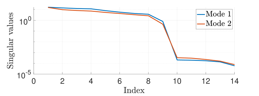
Figure 1: Singular values of data matrices representing restricted behaviors of each mode of system (10).

We propose the following data-driven mode recognition and control strategy. Before starting, let $t\geq 0$ denote the current time, and fix the matrix $D$ in (11). The first step is to compute an SVD of $D$ and form a basis $D_{\textup{basis}}$ using the first ${T_{\textup{ini}}}+{T_{\textup{f}}}+n$ left singular vectors. Next compute an SVD of a matrix with $M$ columns containing the most recent ${T_{\textup{ini}}}+{T_{\textup{f}}}$-length trajectories, denoted $H_{t}$, and form a basis, denoted $H_{t,\textup{basis}}$, using the first ${T_{\textup{ini}}}+{T_{\textup{f}}}+n$ left singular vectors. Fix a threshold $\epsilon>0$. If $\textup{gap}_{{T_{\textup{ini}}}+{T_{\textup{f}}}}(\operatorname{im}H_{t,\textup{basis}},\operatorname{im}D_{\textup{basis}})>\epsilon$, set $D=H_{t}$. This can be thought of as adopting the most recent data as the predictive model in (11) only when the gap between the predictive model $D$ and the most recent data $H_{t}$ is larger than some pre-defined threshold. Equipped with the data matrix $D$, solve (11) for the optimal predicted input trajectory $(u_{1}^{\star},\dots,u_{{T_{\textup{f}}}}^{\star})$ and apply $u_{t}=u_{1}^{\star}$ to the system. Measure $y_{t}$ and set $({u_{\textup{ini}}},{y_{\textup{ini}}})$ in (11) to the most recent ${T_{\textup{ini}}}$-length trajectory of the system. Update $H_{t}$ by deleting the first column and adding the most recent ${T_{\textup{ini}}}+{T_{\textup{f}}}$-length trajectory as the last column. This process is repeated in order to perform simultaneous data-driven mode recognition and control.

The strategy above has been simulated with $\epsilon=0.3$ on system (10) for $t\in[0,70]$. We arbitrarily initialize the predictive model $D$ in (11) to be a matrix containing sufficiently exciting data from mode 1. However, the system starts in mode 2 and only switches to mode 1 at ${t=40}$. The strategy is compared to data-driven control without mode recognition, i.e., where $D$ is kept constant in (11). The results are shown in Figures 2 and 3. We observe in Figure 2 that the controlled output trajectory is offset from the desired reference. This is due to the fact that we are using the wrong data set in (11) for predicting optimal trajectories. However, the $L$-gap between $D_{\textup{basis}}$ and $H_{t,\textup{basis}}$ quickly increases above the threshold $\epsilon$, thus successfully recognizing a discrepancy between the current mode of the system and the data being used for control (see Figure 3). During this transient phase, the moving window contains a mixture of data containing trajectories from mode 2, and mode 1. However, at approximately ${t=22}$, the $L$-gap successfully recognizes that the data matrix $D$ used in (11) is consistent with the current mode of the system (mode 2). The control performance after this transient phase then improves. This is again illustrated during the mode switch at ${t=40}$. On the other hand, the data-driven control strategy with no mode recognition does not adapt to mode switches and has poor performance until ${t=40}$ where the system switches incidentally to mode 1 thus matching with the fixed data matrix $D$ being used in this strategy. This case study suggests that the $L$-gap is a suitable tool for data-driven online mode recognition and control.

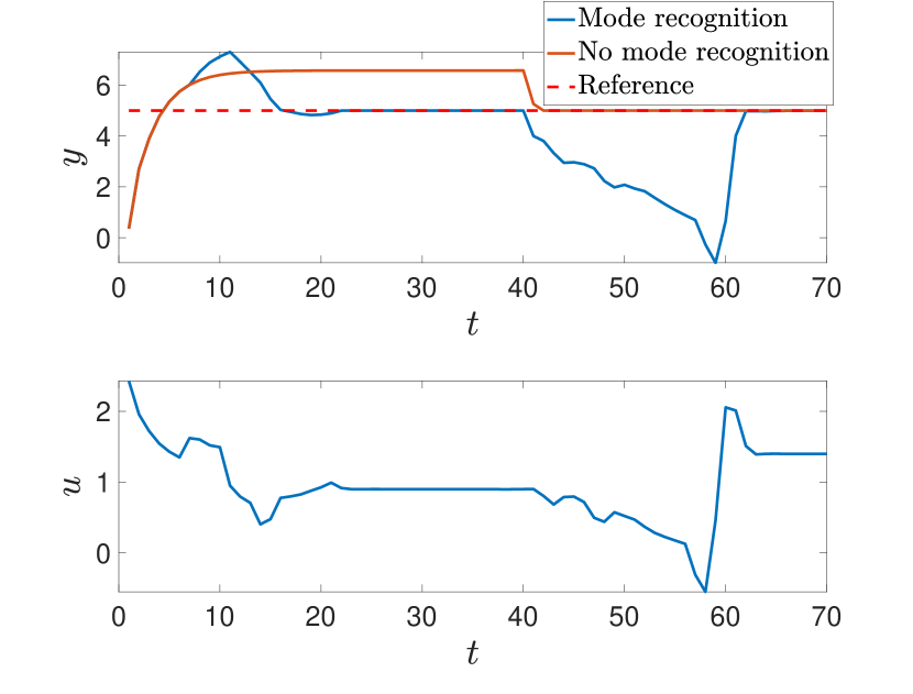
Figure 2: Performance of mode recognition and control strategy on the SARX system with switches between modes compared to data-driven control without mode recognition.

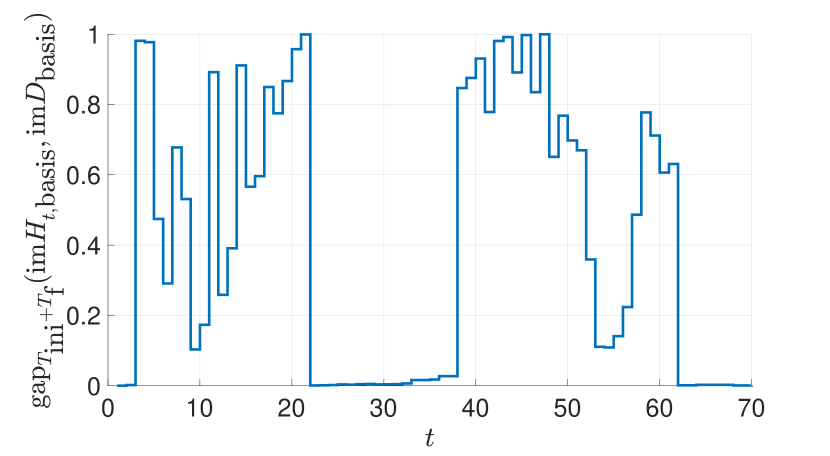
Figure 3: Distance computed with the $L$-gap between $H_{t,\textup{basis}}$ and $D_{\textup{basis}}$ for $L={T_{\textup{ini}}}+{T_{\textup{f}}}$.

V Conclusion

This paper has explored the issue of uncertainty quantification in the behavioral setting. A new metric has been defined on the set of restricted behaviors and shown to capture parametric uncertainty for the class of AR models. The metric is a direct finite-time counterpart of the classical gap metric. A data-driven control case study has illustrated the value of the new metric through numerical simulations.

TABLE I: Metrics between subspaces $\mathcal{V}$ and $\mathcal{W}$ in $\operatorname{Gr}(k,N)$ in terms of the corresponding principal angles $\{\theta_{i}\}_{i\in\mathbf{k}}$ and in terms of matrices $V$ and $W$ whose columns are orthonormal bases for $\mathcal{V}$ and $\mathcal{W}$, with ${V}^{\mathsf{T}}W=USZ^{\mathsf{T}}$ a (full) SVD.

Metric	Principal angles	Matrix representations
Asimov	$d^{\alpha}(\mathcal{V},\mathcal{W})=\theta_{k}$	$\sin^{-1}\left\lVert VV^{\mathsf{T}}-WW^{\mathsf{T}}\right\rVert_{2}$
Binet-Cauchy	$d^{\beta}(\mathcal{V},\mathcal{W})=\left(1-\prod_{i=1}^{k}(\cos\theta_{i})^{2}\right)^{1/2}$	$\left(1-\det(V^{\mathsf{T}}W)^{2}\right)^{1/2}$
Chordal	$d^{\kappa}(\mathcal{V},\mathcal{W})=\left(\sum_{i=1}^{k}(\sin\theta_{i})^{2}\right)^{1/2}$	$\tfrac{1}{\sqrt{2}}\left\lVert VV^{\mathsf{T}}-WW^{\mathsf{T}}\right\rVert_{F}$
Fubini-Study	$d^{\phi}(\mathcal{V},\mathcal{W})=\cos^{-1}\left(\sum_{i=1}^{k}(\cos\theta_{i})\right)$	$\cos^{-1}|\det V^{\mathsf{T}}W|$
Grassmann	$d^{\gamma}(\mathcal{V},\mathcal{W})=\left(\sum_{i=1}^{k}\theta_{i}^{2}\right)^{1/2}$	$\left\lVert\cos^{-1}\Sigma\right\rVert_{F}$
Martin	$d^{\mu}(\mathcal{V},\mathcal{W})=\left(\log\left(\prod_{i=1}^{k}1/(\cos\theta_{i})^{2}\right)\right)^{1/2}$	$(-2\log\det V^{\mathsf{T}}W)^{1/2}$
Procrustes	$d^{\rho}(\mathcal{V},\mathcal{W})=2\left(\sum_{i=1}^{k}(\sin(\theta_{i}/2))^{2}\right)^{1/2}$	$\left\lVert VU-WZ\right\rVert_{F}$
Projection (gap)	$d^{\pi}(\mathcal{V},\mathcal{W})=\sin\theta_{k}$	$\left\lVert VV^{\mathsf{T}}-WW^{\mathsf{T}}\right\rVert_{2}$
Spectral	$d^{\sigma}(\mathcal{V},\mathcal{W})=2\sin(\theta_{k}/2)$	$\left\lVert VU-WZ\right\rVert_{2}$

The paper has shown that the gap induces a metric space structure on the set of restricted behaviors. However, there are many other common metrics defined on Grassmannians [34]. Table I recalls some of these metrics, as well as formulae to compute them. The fact that all distances in Table I depend on the principal angles is not a coincidence. In fact, the geometry of the Grassmannian is such that any rotationally invariant metric between $k$-dimensional subspaces in $\mathbb{R}^{N}$ (i.e., dependent only on the relative the position of subspaces) is necessarily a function of the principal angles.

Theorem 3.

[30, Theorem 2] Let ${d}$ be a rotationally invariant metric on $\operatorname{Gr}(k,N)$. Then $d(\mathcal{V},\mathcal{W})$ is a function of the principal angles $\{\theta_{i}\}_{i\in\mathbf{k}}$ between the subspaces $\mathcal{V}$ and $\mathcal{W}$.

Each metric induces a particular geometry, which comes with its own advantages and disadvantages. For example, the Grassmann metric is the geodesic distance on $\operatorname{Gr}(k,N)$ [30, Theorem 2], viewed as a Riemannian (quotient) manifold with metric ${g_{Z}(V,W)=\operatorname{trace}((Z^{\mathsf{T}}Z)^{-1}V^{\mathsf{T}}W)}$. The corresponding geodesics admit an explicit expression [35], which allows for a number of optimization-based problems to be solved (e.g., regression [36]). This, in turn, suggests that the choice of the metric structure on the set of restricted behaviors is crucial, raising a number of important questions. For instance, any metric on $\operatorname{Gr}(k,N)$ that induces a differentiable structure opens up the possibility of directly optimizing over behaviors. So can one exploit any such structure to improve the performance of data-driven control algorithms (e.g., DeePC)? In practice, non-parametric representations of restricted behaviors are typically constructed from noisy measurements. This can be a serious drawback, because noisy restricted behaviors may appear to be far apart, even when close and/or of the same dimension. This issue may be elegantly resolved by extending the metrics in Table I to infinite Grassmannians [30]. So can one leverage these results in an online, real-time, noisy setting where behaviors are constantly changing? We leave the exploration of these important questions as future research directions.

Appendix A Background

A-A The principal angles

Let ${\mathcal{V}\in\operatorname{Gr}(k,N)}$ and ${\mathcal{W}\in\operatorname{Gr}(l,N)}$. Let ${r=\min(k,l)}$. For ${i\in\mathbf{r}}$, the $i$-th principal vectors $(p_{i},q_{i})$ are defined, recursively, as the solution of the optimization problem

$$\begin{array}[]{ll}\mbox{maximize}&p^{\mathsf{T}}q\\ \mbox{subject to}&p\in\mathcal{V},~{}p^{\mathsf{T}}p_{1}=\ldots=p^{\mathsf{T}}p_{i-1}=0,\ \,\left\lVert p\right\rVert_{2}=1,\\ &q\in\mathcal{W},\ q^{\mathsf{T}}q_{1}=\ldots=q^{\mathsf{T}}q_{i-1}=0,\ \,\left\lVert q\right\rVert_{2}=1.\end{array}$$

The principal angles between the subspaces ${\mathcal{V}}$ and ${\mathcal{W}}$ are defined as ${\theta_{i}=\arccos(p_{i}^{\mathsf{T}}q_{i})}$ for ${i\in\mathbf{r}}$. Clearly, ${0\leq\theta_{1}\leq\ldots\leq\theta_{r}\leq\tfrac{\pi}{2}}$. Principal vectors and principal angles may be easily computed using, e.g., the SVD [29]. Let ${V\in\mathbb{R}^{N\times k}}$ and ${W\in\mathbb{R}^{N\times l}}$ be a $k$-frame of ${\mathcal{V}\in\operatorname{Gr}(k,N)}$ and an $l$-frame of ${\mathcal{W}\in\operatorname{Gr}(l,N)}$, respectively. Let ${{V}^{\mathsf{T}}W=USZ^{\mathsf{T}}}$ be a (full) SVD of the matrix ${V}^{\mathsf{T}}W$, i.e. , ${U\in\operatorname{O}(k)}$, ${V\in\operatorname{O}(l)}$, ${S=\operatorname{block-diag}(S_{1})\in\mathbb{R}^{k\times l}}$ with $S_{1}=\operatorname{diag}(\sigma_{1},\ldots,\sigma_{r})\in\mathbb{R}^{r\times r}$, where $\sigma_{1}\geq\ldots\geq\sigma_{r}\geq 0$. The principal angles can be computed as ${\theta_{i}=\arccos(\sigma_{i}),}$ with ${i\in\mathbf{r}}$. See [29] for further detail.

A-B Proof of Theorem 2

The proof of the theorem requires some preliminary results. We first establish a one-to-one correspondence between $\mathbb{R}^{qL}$ and the subspace of $\mathbb{R}^{q}$-valued sequences with finitely many non-zero elements, as well as additional elementary results (omitting the proof of those that may be established by direct computation).

Let $(\mathbb{R}^{q})^{\infty}$ be the space of $\mathbb{R}^{q}$-valued sequences with finitely many non-zero elements, i.e., $(\mathbb{R}^{q})^{\infty}=\{w\in(\mathbb{R}^{q})^{\mathbb{Z}_{+}}\,:\,\exists\,T\in\mathbb{Z}_{+}\text{ s.t. }{w_{t}=0},\,\forall\,t\geq T\}.$ For ${L\in\mathbb{N}}$, let ${\iota_{L}:\mathbb{R}^{qL}\to(\mathbb{R}^{q})^{\infty}}$ be the inclusion map, defined as $\iota_{L}(w)=\left(w_{1},\ldots,w_{L},0,0,\ldots\right).$ Then we have $(\mathbb{R}^{q})^{\infty}=\bigcup_{L=0}^{\infty}\iota_{L}(\mathbb{R}^{qL}).$ Thus, each image $\iota_{L}(\mathbb{R}^{qL})$ may be identified with $\mathbb{R}^{qL}$ by identifying each $\left(w_{1},\ldots,w_{L},0,0,\ldots\right)\in(\mathbb{R}^{q})^{\infty}$ with ${w=\text{col}\left(w_{1},\ldots,w_{L}\right)\in\mathbb{R}^{qL}}$. Furthermore, the subspace topology on $\iota_{L}(\mathbb{R}^{qL})$, the quotient topology induced by the map $\iota_{L}$, and the Euclidean topology on $\mathbb{R}^{qL}$, all coincide.

Lemma 4.

Let ${w\in\mathbb{R}^{qL}}$. Then ${\iota_{L}(w)\in\ell_{2}^{q}}$ and ${\left\lVert w\right\rVert_{2}=\left\lVert\iota_{L}(w)\right\rVert_{\ell_{2}}}.$

Lemma 5.

Let $\mathcal{S}$ be a subset of a topological space and let $f:\mathcal{S}\to\mathbb{R}$ be a continuous function. Assume ${\mathcal{S}_{0}\subseteq\mathcal{S}_{1}\subseteq\ldots}$ is a sequence of subsets of $\mathcal{S}$ such that ${\mathcal{S}\subseteq\operatorname{cl}\left(\bigcup_{L=0}^{\infty}\mathcal{S}_{L}\right)}$ then $\sup_{\mathcal{S}}f=\lim_{L\to\infty}\sup_{\mathcal{S}_{L}}f,$ whenever the limit exists.

Proof.

The sequence $\sup_{\mathcal{S}_{L}}f$ is non-decreasing, so $\lim_{L\to\infty}\sup_{\mathcal{S}_{L}}f=\sup_{L\in\mathbb{Z}_{+}}\sup_{\mathcal{S}_{L}}f.$ Furthermore, by assumption, ${\mathcal{S}_{L}\subseteq\mathcal{S}}$ for every ${L\in\mathbb{Z}_{+}}$, so $\sup_{\mathcal{S}}f\geq\sup_{L\in\mathbb{Z}_{+}}\sup_{\mathcal{S}_{L}}f.$ To prove the reverse inequality, consider a sequence ${w_{L}}\in\mathcal{S}$ such that ${f(w_{L})\to\sup_{\mathcal{S}}f}$. Then, for every ${L\in\mathbb{Z}_{+}}$ there is ${\epsilon_{L}>0}$ such that ${f(w)>f(w_{L})-1/L}$ for every ${w\in\mathcal{N}_{\epsilon_{L}}(w_{L})}$, with $\mathcal{N}_{\epsilon_{L}}(w_{L})$ an $\epsilon_{L}$-neighborhood of $w_{L}$. By assumption, ${\mathcal{S}\subseteq\operatorname{cl}\left(\bigcup_{L=1}^{\infty}\mathcal{S}_{L}\right)}$, so every $\mathcal{N}_{\epsilon_{L}}(w_{L})$ contains a point $\bar{w}_{L}\in\mathcal{S}_{k_{L}}$ for some $\mathcal{S}_{k_{L}}$. Thus, $f(\bar{w}_{L})\to\sup_{\mathcal{S}}f$. This, in turn, implies $\sup_{\mathcal{S}}f\leq\sup_{L\in\mathbb{Z}_{+}}\sup_{\mathcal{S}_{L}}f.$ ∎

Given ${L\in\mathbb{Z}_{+}}$, let ${\Pi_{L}:(\mathbb{R}^{q})\to(\mathbb{R}^{q})^{\mathbb{Z}_{+}}}$ be the truncation operator, defined as [37, p.13]

$$\Pi_{L}(w)=\begin{cases}w_{t},&\text{ for }t\in[0,L-1]\cap\mathbb{Z}_{+},\\ 0,&\text{ otherwise},\end{cases}$$

with the convention that ${\Pi_{0}(w)=w}$ for all ${w\in(\mathbb{R}^{q})^{\mathbb{Z}_{+}}}$.

Lemma 6.

Let $\mathcal{B}\in\mathcal{L}^{q}$. Then ${\iota_{L}(\mathcal{B}|_{L})=\Pi_{L}(\mathcal{B})}.$

Lemma 7.

Let $\mathcal{B}\in\mathcal{L}^{q}\cap\ell_{2}^{q}$. Then ${\mathcal{B}=\operatorname{cl}\left(\bigcup_{L=0}^{\infty}\Pi_{L}(\mathcal{B})\right)}.$

Proof.

($\subseteq$). Since ${\mathcal{B}\cap(\mathbb{R}^{q})^{\infty}=\bigcup_{L=0}^{\infty}\Pi_{L}(\mathcal{B})}$, we have

$$\operatorname{cl}\left(\bigcup_{L=0}^{\infty}\Pi_{L}(\mathcal{B})\right) =\operatorname{cl}\left(\mathcal{B}\cap(\mathbb{R}^{q})^{\infty}\right)\subseteq\operatorname{cl}(\mathcal{B})\cap\operatorname{cl}\left((\mathbb{R}^{q})^{\infty}\right)$$

$$=\operatorname{cl}(\mathcal{B})\cap(\mathbb{R}^{q})^{\mathbb{Z}_{+}}=\operatorname{cl}(\mathcal{B})=\mathcal{B},$$

where we have used ${(\mathbb{R}^{q})^{\mathbb{Z}_{+}}=\operatorname{cl}\left((\mathbb{R}^{q})^{\infty}\right)}$ [38, p151] and the completeness of $\mathcal{B}$.

($\supseteq$). Let ${w\in\mathcal{B}}$ and recall that ${w\in\operatorname{cl}\left(\bigcup_{L=0}^{\infty}\Pi_{L}(\mathcal{B})\right)}$ if and only if ${w}$ is the limit of some sequence of points in ${\bigcup_{L=0}^{\infty}\Pi_{L}(\mathcal{B})}$. Consider the sequence $\bar{w}_{L}=\Pi_{L}(w)$ for $L\in\mathbb{Z}_{+}$. Clearly, ${\bar{w}_{L}\in{\bigcup_{L=0}^{\infty}\Pi_{L}(\mathcal{B})}}$. Furthermore, since ${\mathcal{B}\in\mathcal{L}^{q}\cap\ell_{2}^{q}}$, ${\bar{w}_{L}\to w}$, as desired. ∎

Proof of Theorem 2.

By assumption, $P$ and $\tilde{P}$ are bounded linear operators, so $\text{gap}_{\ell_{2}}(P,\tilde{P})$ is well-defined. Then

$$\lim_{L\to\infty}\overset{\rightharpoonup}{\text{gap}}_{L}(\mathcal{B},\tilde{\mathcal{B}}) \stackrel{{\scriptstyle\eqref{eq:gapL_def}}}{{=}}\lim_{L\to\infty}\overset{\rightharpoonup}{\text{gap}}(\mathcal{B}|_{L},\tilde{\mathcal{B}}|_{L})$$

$$\stackrel{{\scriptstyle\eqref{eq:directed_gap}}}{{=}}\lim_{L\to\infty}\sup_{w\in\mathcal{B}|_{L}\atop\left\lVert w\right\rVert_{2}=1}\inf_{\tilde{w}\in\tilde{\mathcal{B}}|_{L}}\left\lVert w-\tilde{w}\right\rVert_{2}$$

$$=\lim_{L\to\infty}\sup_{w\in\iota_{L}(\mathcal{B}|_{L})\atop\left\lVert w\right\rVert_{\ell_{2}}=1}\inf_{\tilde{w}\in\iota_{L}(\tilde{\mathcal{B}}|_{L})}\left\lVert w-\tilde{w}\right\rVert_{\ell_{2}}$$

$$=\lim_{L\to\infty}\sup_{w\in\Pi_{L}(\mathcal{B}))\atop\left\lVert w\right\rVert_{\ell_{2}}=1}\inf_{\tilde{w}\in\Pi_{L}(\tilde{\mathcal{B}})}\left\lVert w-\tilde{w}\right\rVert_{\ell_{2}}$$

$$\leq\lim_{L\to\infty}\sup_{w\in\Pi_{L}(\mathcal{B}))\atop\left\lVert w\right\rVert_{\ell_{2}}=1}\inf_{\tilde{w}\in\tilde{\mathcal{B}}}\left\lVert w-\tilde{w}\right\rVert_{\ell_{2}}$$

$$=\sup_{w\in\mathcal{B}\atop\left\lVert w\right\rVert_{\ell_{2}}=1}\inf_{\tilde{w}\in\tilde{\mathcal{B}}}\left\lVert w-\tilde{w}\right\rVert_{\ell_{2}}$$

$$=\overset{\rightharpoonup}{\text{gap}}_{\ell_{2}}(P,\tilde{P}),$$ (12)

where the third identity is a consequence of Lemma 4, the fourth identity follows from Lemma 6, the fifth inequality is implied by ${\inf_{\tilde{w}\in\Pi_{L}(\tilde{\mathcal{B}})}\left\lVert w-\tilde{w}\right\rVert_{\ell_{2}}\leq\inf_{\tilde{w}\in\tilde{\mathcal{B}}}\left\lVert w-\tilde{w}\right\rVert_{\ell_{2}}}$ for ${w\in\Pi_{L}(\mathcal{B})}$, the sixth equality is a consequence of Lemma 5, and the last identity holds by Definition 9, since ${\mathcal{B}=\text{graph}_{\ell_{2}}(P)}$ and ${\mathcal{B}=\text{graph}_{\ell_{2}}(\tilde{P})}$, by assumption. Finally, the function $(x,y)\mapsto\max(x,y)$ is continuous, thus

$$\lim_{L\to\infty}{\text{gap}}_{L}(\mathcal{B},\tilde{\mathcal{B}}) =\lim_{L\to\infty}\max\{\overset{\rightharpoonup}{\text{gap}}_{L}(\mathcal{B},\tilde{\mathcal{B}}),\overset{\rightharpoonup}{\text{gap}}_{L}(\tilde{\mathcal{B}},\mathcal{B})\}$$

$$\stackrel{{\scriptstyle\eqref{eq:proof_thm_connection}}}{{\leq}}\max\{\overset{\rightharpoonup}{\text{gap}}_{\ell_{2}}(P,\tilde{P}),\overset{\rightharpoonup}{\text{gap}}_{\ell_{2}}(\tilde{P},P)\}$$

$$={\text{gap}}_{\ell_{2}}(\tilde{P},P).$$

∎

References

- [1] L. Ljung, System identification - Theory for the user (2nd edition). Upper Saddle River, NJ, USA: Prentice-Hall, 1999.
- [2] P. Van Overschee and B. De Moor, Subspace identification for linear systems: theory - implementation - applications. Dordrecht, The Netherlands: Kluwer, 1996.
- [3] J. C. Willems, P. Rapisarda, I. Markovsky, and B. L. M. De Moor, “A note on persistency of excitation,” Syst. Control Lett., vol. 54, no. 4, pp. 325–329, 2005.
- [4] J. C. Willems, “From time series to linear system—Part I. Finite dimensional linear time invariant systems,” Automatica, vol. 22, no. 5, pp. 561–580, 1986.
- [5] J. C. Willems and J. W. Polderman, Introduction to mathematical systems theory: a behavioral approach. New York, NY, USA: Springer, 1997.
- [6] J. Coulson, J. Lygeros, and F. Dörfler, “Data-enabled predictive control: In the shallows of the deepc,” in Proc. Eur. Control Conf., Naples, Italy, 2019, pp. 307–312.
- [7] C. De Persis and P. Tesi, “Formulas for data-driven control: Stabilization, optimality, and robustness,” IEEE Trans. Autom. Control, vol. 65, no. 3, pp. 909–924, 2019.
- [8] H. J. van Waarde, J. Eising, H. L. Trentelman, and M. K. Camlibel, “Data informativity: a new perspective on data-driven analysis and control,” IEEE Transactions on Automatic Control, vol. 65, no. 11, pp. 4753–4768, 2020.
- [9] I. Markovsky and F. Dörfler, “Behavioral systems theory in data-driven analysis, signal processing, and control,” Ann. Rev. Control, vol. 52, pp. 42–64, 2021.
- [10] J. Coulson, J. Lygeros, and F. Dörfler, “Distributionally robust chance constrained data-enabled predictive control,” IEEE Trans. Autom. Control, 2021.
- [11] P. G. Carlet, A. Favato, S. Bolognani, and F. Dörfler, “Data-driven predictive current control for synchronous motor drives,” in IEEE Energy Conversion Congress and Exposition, Detroit, MI, USA, 2020, pp. 5148–5154.
- [12] L. Huang, J. Coulson, J. Lygeros, and F. Dörfler, “Data-enabled predictive control for grid-connected power converters,” in Proc. 58th Conf. Decision Control, Naples, Italy, 2019, pp. 8130–8135.
- [13] J. Berberich, A. Koch, C. W. Scherer, and F. Allgöwer, “Robust data-driven state-feedback design,” in Proc. Amer. Control Conf., Denver, CO, USA, 2020, pp. 1532–1538.
- [14] H. J. van Waarde, M. K. Camlibel, and M. Mesbahi, “From noisy data to feedback controllers: Nonconservative design via a matrix S-lemma,” IEEE Transactions on Automatic Control, vol. 67, no. 1, pp. 162–175, 2022.
- [15] A. Xue and N. Matni, “Data-driven system level synthesis,” in Learning for Dynamics and Control. PMLR, 2021, pp. 189–200.
- [16] A. Bisoffi, C. De Persis, and P. Tesi, “Data-driven control via Petersen’s lemma,” arXiv:2109.12175, 2021.
- [17] L. Huang, J. Zhen, J. Lygeros, and F. Dörfler, “Robust data-enabled predictive control: Tractable formulations and performance guarantees,” arXiv preprint arXiv:2105.07199, 2021.
- [18] G. Zames and A. El-Sakkary, “Uncertainty in unstable systems: The gap metric,” in Proc. 8th IFAC World Congr., vol. 14, no. 2, 1981, pp. 149–152.
- [19] J. R. Partington, Linear operators and linear systems: an analytical approach to control theory. Cambridge, U. K.: Cambridge Univ. Press, 2004.
- [20] K. Zhou, J. C. Doyle, and K. Glover, Robust and optimal control. New Jersey, NJ, USA: Prentice Hall, 1996.
- [21] G. Vinnicombe, Uncertainty and feedback: loop-shaping and the -gap metric. London, U.K.: Imperial College Press, 2001.
- [22] F. Dorfler, J. Coulson, and I. Markovsky, “Bridging direct & indirect data-driven control formulations via regularizations and relaxations,” IEEE Trans. Autom. Control, 2022.
- [23] K. J. Åström and B. Wittenmark, Adaptive control (2nd edition). Reading, MA, USA: Addison-Wesley, 1995.
- [24] I. Markovsky and F. Dörfler, “Identifiability in the behavioral setting,” Vrije Universiteit Brussel, Tech. Rep, 2020. [Online]. Available: {http://homepages.vub.ac.be/~imarkovs/publications/identifiability.pdf.}
- [25] W. M. Boothby, An introduction to differentiable manifolds and Riemannian geometry (2nd Edition). London, U. K.: Academic Press, 1986.
- [26] N. L. Carothers, Real analysis. Cambridge, U. K.: Cambridge Univ. Press, 2000.
- [27] T. Kato, Perturbation theory for linear operators (2nd Edition). New York, NY, USA: Springer, 1980.
- [28] G. Stewart and J. Sun, Matrix Perturbation Theory. New York, NY, USA: Academic Press, 1990.
- [29] G. H. Golub and C. F. Van Loan, Matrix computations (4th Ed.). Baltimore, MD, USA: Johns Hopkins Univ. Press, 2013.
- [30] K. Ye and L. H. Lim, “Schubert varieties and distances between subspaces of different dimensions,” SIAM J. Mat. Anal. Appl., vol. 37, no. 3, pp. 1176–1197, 2016.
- [31] L. Qui and E. J. Davison, “Pointwise gap metrics on transfer matrices,” IEEE Trans. Autom. Control, vol. 37, no. 6, pp. 741–758, 1992.
- [32] T. Koenings, M. Krueger, H. Luo, and S. X. Ding, “A data-driven computation method for the gap metric and the optimal stability margin,” IEEE Trans. Autom. Control, vol. 63, no. 3, pp. 805–810, 2017.
- [33] Z. Du, L. Balzano, and N. Ozay, “A robust algorithm for online switched system identification,” IFAC-PapersOnLine, vol. 51, no. 15, pp. 293–298, 2018.
- [34] M. M. Deza and E. Deza, Encyclopedia of distances. New York, NY, USA: Springer, 2009.
- [35] P. A. Absil, R. Mahony, and R. Sepulchre, Optimization algorithms on matrix manifolds. Princeton, NJ, USA: Princeton Univ. Press, 2009.
- [36] Y. Hong, R. Kwitt, N. Singh, B. Davis, N. Vasconcelos, and M. Niethammer, “Geodesic regression on the grassmannian,” in Eur. Conf. Comp. Vision. Springer, 2014, pp. 632–646.
- [37] J. C. Willems, The analysis of feedback systems. London, U. K.: MIT Press, 1971.
- [38] J. R. Munkres, Topology (2nd Edition). Upper Saddle River, NJ, USA: Prentice Hall, 2000.