Spatio-Temporal Dynamic Graph Relation Learning for Urban Metro Flow Prediction

Abstract

Urban metro flow prediction is of great value for metro operation scheduling, passenger flow management and personal travel planning. However, it faces two main challenges. First, different metro stations, e.g. transfer stations and non-transfer stations, have unique traffic patterns. Second, it is challenging to model complex spatio-temporal dynamic relation of metro stations. To address these challenges, we develop a spatio-temporal dynamic graph relational learning model (STDGRL) to predict urban metro station flow. First, we propose a spatio-temporal node embedding representation module to capture the traffic patterns of different stations. Second, we employ a dynamic graph relationship learning module to learn dynamic spatial relationships between metro stations without a predefined graph adjacency matrix. Finally, we provide a transformer-based long-term relationship prediction module for long-term metro flow prediction. Extensive experiments are conducted based on metro data in Beijing, Shanghai, Chongqing and Hangzhou. Experimental results show the advantages of our method beyond 11 baselines for urban metro flow prediction.

1 Introduction

As a significant part of urban public transportation, the urban metro takes a large proportion of urban traffic. Especially for large cities, accurate prediction of urban metro passenger flow is significant for metro operation scheduling [1], passenger flow management [2], and personal travel planning [3]. The urban metro network is a spatio-temporal dynamic graph with prominent spatial and temporal characteristics. We show the change of passenger outflow for three different metro stations over the time frame of one day in Figure 1(a). We can observe that the passenger outflow of station 1 has a small peak between 7:00 and 9:00 in the morning, and there is also a small evening peak period between 17:00 and 19:00. While station 2 only has a relatively small period of passenger flow between 7:00 and 9:00 in the morning, there is no obvious evening peak at night, and the overall one-day passenger outflow is smaller than that of station 1. Station 3 has a large peak in passenger outflow between 7:00 and 9:00, and then the passenger outflow at other periods decreases significantly. Still, the overall passenger flow of station 3 is much larger than those of stations 1 and 2. We can see that these stations have their own different station traffic patterns, not just a simple, fixed spatial connection relationship between stations. Different metro stations are connected and affected each other. This spatial dependency relationship changes dynamically along with time and location as shown in Figure 1(b).

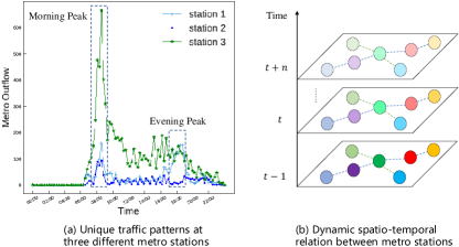
Figure 1: Spatio-temporal dynamic graph relation. (a) The metro outflow of station 1 has a prominent morning peak and evening peak. As a contrast, station 2 only has a morning peak and station 3 has an extremely big morning peak. It shows unique traffic patterns at three different metro stations. (b) These stations are connected to each other, the passengers’ inflow and outflow of metro stations change over time, there are dynamic spatio-temporal dependency relations between stations.

In order to achieve the prediction of passenger flow in metro stations, some research works have been tried and studied [4, 5, 6, 7]. Most of these methods model the flow change trend of metro stations according to inflow and outflow passenger data, metro network topology map, weather, and other external factors. Most of them use CNN and GNN-based methods to capture spatial dependencies in metro flow data [8], and apply RNN-based and Attention-based methods to model the temporal dependencies of metro traffic data [9], and some research take external factors into account [6]. These studies have made some progress, but most of these works only use a single metro traffic data set or need to predefine the adjacency relationship between stations. Others treat different stations in the metro network as the same kind of node. Overall, the generalization performance of these models is insufficient.

In summary, the urban metro flow prediction task faces three major challenges:

1) Modeling unique traffic patterns at different stations: Previous research [8, 10, 11] has treated metro stations as equal nodes or divided metro stations into transfer stations and non-transfer stations. The parameters are shared globally or locally when using a static adjacency matrix, and the computational cost is relatively small. Still, it ignores the traffic flow patterns differences between different stations. However, we find that although different stations are directly connected or are all transfer stations, they have unique traffic change patterns, as shown in Figure 1(a). Therefore, it is necessary to model the traffic patterns of different stations separately.

2) Dynamic spatial dependency relations between stations: The spatial dependencies between stations are regarded as static in the existing work [8, 12, 6]. Some of them express their spatial dependencies directly with the existence or lack of connections between stations. The distance between them and the similarity of traffic flow is regarded as spatial dependencies. But this method is viewed as static, which ignores that the passenger inflow and outflow of a station are not only affected by the passenger flow of its upstream, downstream stations and nearby stations, but also by time, weather and other factors. Therefore, it’s a challenge to capture the dynamic spatial dependency relation between stations.

3) Long-term temporal prediction: To better support the downstream applications of the metro, it is necessary to carry out a long-term metro station flow prediction. Existing research [6] on short-term metro station passenger flow prediction has been carried out. Still, there is a lack of relevant research on long-term accurate metro station flow prediction because long-term time series forecasting is challenging. As the prediction period becomes longer, the influence of uncertain factors will reduce prediction accuracy, and the dynamic variability of the metro flow itself also increases the uncertainty of metro flow prediction. In general, compared with short-term prediction, long-term prediction is more difficult but has greater practical application value.

In order to cope with the above challenges, we propose a spatio-temporal dynamic graph relation learning method for metro flow prediction, which can model different traffic patterns at different stations and capture the dynamic spatial dependency relation between stations. At the same time, it can carry out long-term prediction, which can better support traffic management of metro operation managers and travel decisions of urban residents. The contributions of this paper include four aspects, as follows:

• A node-adaptive parameter learning module is adopted to learn different station-specific spatiotemporal embedding representations to capture the flow patterns of different stations.

• A dynamic graph relation learning module is proposed to learn the dynamic spatial dependencies between stations, which does not require a predefined spatial relationship of station connections, and directly learn the dynamic spatial dependencies between stations from the spatiotemporal graph data.

• A long-term temporal relation prediction module based on Transformer is used to predict the long-term metro flow. The predicted results can offer a useful reference for urban metro operation management and personal travel planning.

• Experiments are conducted on 4 different cities’ metro datasets, including Beijing, Shanghai, Chongqing, Hangzhou. Compared with the 11 baseline methods, the experimental results have significantly improved prediction performance.

The remainder of this paper is organized as follows. In Section 2, we present the related work about urban flow prediction and graph neural networks. In Section 3, we introduce some preliminary concepts and formalize the metro flow prediction problem. In Section 4, we show the overall framework of the proposed STDGRL model. The experiment result, visualization and analysis are given in Section 5. We conclude the work in Section 6.

2 Related Work

2.1 Urban Flow Prediction

Urban flow prediction is important for traffic management[13], land use[14], public safety[15], etc. The urban flow prediction can be regarded as a spatio-temporal prediction task, which is a kind of research problem that uses spatio-temporal machine learning methods to learn spatio-temporal correlations from spatio-temporal datasets[16]. At present, a large number of researchers have conducted studies on the task of urban flow prediction. Xie et al.[17] divided the urban flow prediction task into crowd flow prediction, traffic flow prediction, and public transport flow prediction and reviewed the classical deep learning methods. With the city’s continuous development, more and more people are pouring into the city, and the metro and other public transportations occupy the main body of the urban traffic flow. Accurate metro flow prediction is of great value for urban traffic management, urban public safety, and residents’ daily travel. In the early work, researchers used statistical-based methods for urban flow prediction, such as ARIMA (Autoregressive Integrated Moving Average)[18], SARIMA (Seasonal Auto-Regressive Integrated Moving Average)[19] and other methods. Later, some classic machine learning methods were used for urban flow prediction, such as SVR(Support Vector Regression)[20], K-NN(K-nearest neighbor)[21] and other methods. But these methods often ignored spatiotemporal correlations are hinted in spatiotemporal data, which are crucial for accurate urban flow prediction.

In recent years, with the development of deep learning, deep learning methods have been used in the research field of urban flow prediction. The representative works mainly include the time series method represented by RNN[22], the spatial relation method represented by CNN[23], and a spatiotemporal relationship method combining the two[24, 25, 9]. Based on RNN and its variant series, these methods focus on capturing temporal dependencies in spatio-temporal data, such as closeness, periodicity, trend, etc[15]. These CNN-based methods mainly capture the spatial dependencies in spatiotemporal data, such as spatial distance, spatial hierarchy, and regional functional similarity[26]. In addition, such methods combining RNN and CNN consider both temporal and spatial dependencies and propose hybrid models to model the spatiotemporal characteristics in traffic data[27].

Later, due to the rise and continuous development of the graph neural network[28, 29, 30] and the graph structure of the road network and rail transit network, more and more researchers have used GNN-based methods for urban flow prediction tasks[31, 32, 33] and achieved good results.

2.2 Graph Neural Networks

Graph neural networks can model graph data in non-Euclidean space, especially the dependencies between nodes. Wu et al. [34] divided graph neural network methods into graph convolutional networks, graph attention networks, graph autoencoders, graph generation networks, and graph spatiotemporal networks. Applying the graph neural network to urban flow prediction, traffic forecasting, and other fields is natural. Since the road network and rail transit network can be regarded as the road segments and stations in the graph, the graph spatiotemporal network can be used to capture the relationship between the nodes. Based on RNN and CNN, the spatial and temporal dependencies in the spatio-temporal graph can be learned, making more accurate traffic state predictions. Among them, two representative works use GCN and RNN[32], GCN and CNN[33] methods to model the spatiotemporal dependencies of spatiotemporal graph data, which are applied to traffic prediction tasks.

However, the previous methods using GNNs for spatiotemporal prediction tasks mostly use a predefined graph structure or a single fixed graph adjacency matrix[35] or multiple graph adjacency matrices for fusion[12]. This type of method regards the spatial dependence in spatiotemporal data as static and invariant. However, in reality, the spatiotemporal relationship in spatio-temporal data is dynamic. It is necessary to model the dynamic graph relationship in spatio-temporal data and capture the spatio-temporal dynamics. Compared with previous methods, our method mainly learns the dynamic graph relationship in the spatiotemporal data to obtain more accurate traffic prediction results.

3 Problem Formulation

This paper proposes a spatio-temporal dynamic graph relation learning model for flow prediction in metro stations. Our model does not need a predetermined metro network topology map, and can directly learn spatial dependencies from metro flow data, which has broad applicability to metro flow prediction tasks in different cities.

Before introducing our model in detail, we first define and represent the metro flow prediction task and related conceptual notations. At station $i$, the metro flow of time period $t$ can be expressed as $\boldsymbol{X}_{i,t}\in\mathbb{R}^{2}$, which includes the passenger inflow and outflow. The flow information of the entire metro network can be expressed as $\boldsymbol{X}_{:,t}=(\boldsymbol{X}_{1,t},\boldsymbol{X}_{2,t},...,\boldsymbol{X}_{N,t})\in\mathbb{R}^{N\times 2}$, where $N$ means the number of metro stations. The metro flow in this paper contains two perspectives, which are passengers inflow and outflow in metro stations. The metro station flow prediction task can be defined as, given the historical flow sequence, predicting the flow sequence for a period of time in the future.

$$X_{:,t+1},X_{:,t+2},\ldots,X_{:,t+m}=\mathcal{F}_{\theta}\left(X_{:,t},X_{:,t-1},\ldots,X_{:,t-T+1}\right),$$ (1)

where $\theta$ means all the learnable parameters in the STDGRL model, $T$ is the length of the input flow sequence, and $m$ means the length of the predicted flow sequence.

4 Methodology

The overall architecture of the model is shown in Figure 2. It contains a node-specific spatiotemporal embedding module, a dynamic spatial relationship learning module, a long-term temporal prediction module and a spatio-temporal fusion module. First, we propose a node-specific spatio-temporal embedding module to embed and represent the stations of the metro spatio-temporal graph. Then we adopt a dynamic spatial relationship learning module to learn the spatial dependencies directly from the metro flow data without relying on a specific metro network topology. Finally, a Transformer-based long-time-series dependency prediction module is used to predict the metro flow in a long-term sequence, making its prediction more suitable for actual metro dispatch management and daily operation scenarios.

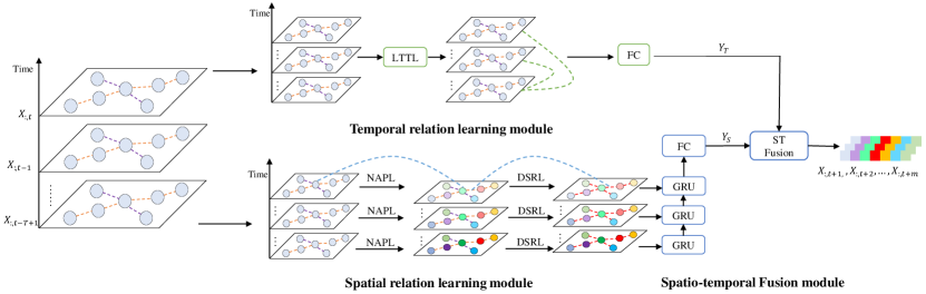
Figure 2: Spatio-Temporal Dynamic Graph Relation Learning (STDGRL) model.

4.1 Node-specific Spatio-Temporal Embedding

The node-specific adaptive parameter learning module (NAPL) is adopted. The classic graph convolution operation [30] is calculated by the following formula:

$$Z=\left(I_{N}+D^{-\frac{1}{2}}AD^{-\frac{1}{2}}\right)X\Theta+b,$$ (2)

where $\boldsymbol{A}\in R^{N\times N}$ is the adjacency matrix of the graph, $D$ is the degree matrix, $I_{N}$ is the identity matrix, $\mathrm{X}\in R^{N\times C}$ is the input of the graph convolutional network layer, $Z\in R^{N\times F}$ is the output of the graph convolutional network layer, $\Theta\in R^{C\times F}$ and $\mathbf{b}\in R^{F}$ represent learnable weights and biases, respectively.

In this method, all nodes on the graph share parameters such as weights and biases. According to the viewpoint put forward by [36], different nodes have different traffic flow patterns, as shown in Figure 1(a), because different nodes have different attributes, such as POI distribution around the nodes, various weather conditions, and different flow patterns will be formed. For more accurate traffic prediction, it is necessary to learn different traffic patterns for different nodes, that is, to learn node-specific patterns by using different learnable parameters rather than globally shared parameters.

In order to learn node-specific patterns, a node-specific adaptive parameter learning module is proposed, which learns the node embedding matrix $E_{\mathcal{G}}\in R^{N\times d}$ and weight pool $W_{\mathcal{G}}\in R^{d\times C\times F}$. The $\Theta$ in the formula 2 can be calculated by the node embedding matrix and the weight pool, $\Theta=E_{\mathcal{G}}\cdot W_{\mathcal{G}}$. Such a computation can be interpreted as learning node-specific patterns from all station time-series patterns. The bias $b$ can also be calculated in the same way. The parameter module of the final node adaptation can be expressed by the formula 3.

$$Z=\left(I_{N}+D^{-\frac{1}{2}}AD^{-\frac{1}{2}}\right)XE_{\mathcal{G}}W_{\mathcal{G}}+E_{\mathcal{G}}\mathrm{b}_{\mathcal{G}}.$$ (3)

4.2 Dynamic Spatial Relation Learning

In the metro network, the connection relationship between stations is fixed and static, as shown in Figure 3. However, this fixed and static connection relationship cannot reflect the dynamic spatial dependence between stations, and with the variation of time, the passengers’ inflow and outflow of stations change, so it is necessary to learn this dynamic spatial dependency from spatiotemporal data. Therefore, a dynamic spatial relationship learning module (DSRL) is proposed, a representation model with adaptive and spatial structure awareness. Inspired by [36], we first randomly initialize a learnable node embedding dictionary $E_{A}\in R^{N\times d_{e}}$ for all nodes. During the model training process, $E_{A}$ will be dynamically updated. Each row of $E_{A}$ represents the embedding representation of the node, and $d_{e}$ represents the dimension of node embedding. Then, the spatial dependency between nodes is calculated by multiplying $E_{A}$ and $E_{A}^{T}$. Finally, we can get the generated graph Laplacian matrix as shown in the formula below.

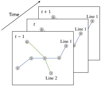
Figure 3: Static spatial relation between metro stations.

$$D^{-\frac{1}{2}}AD^{-\frac{1}{2}}=softmax(ReLU(E_{A}\cdot E_{A}^{T})),$$ (4)

where the $softmax$ function is used to normalize the learned adaptive matrix. The calculation formula of GCN is as follows:

$$Z=(I_{N}+softmax(ReLU(E_{A}\cdot E_{A}^{T})))X\Theta+b.$$ (5)

For the nodes at time step $t$, the operation of the GRU module can be expressed as follows:

$$\widetilde{A}=\operatorname{softmax}\left(\operatorname{ReLU}\left(\boldsymbol{E_{A}}\boldsymbol{E_{A}^{\boldsymbol{T}}}\right)\right),$$ (6)

$$z_{t}=\sigma_{z}\left(\widetilde{\boldsymbol{A}}\left[\boldsymbol{X}_{:,t},h_{t-1}\right]\boldsymbol{E}\boldsymbol{W}_{\boldsymbol{z}}+\boldsymbol{E}\boldsymbol{b}_{\boldsymbol{z}})\right.,$$

$$r_{t}=\sigma_{r}\left(\widetilde{\boldsymbol{A}}\left[\boldsymbol{X}_{:,t},h_{t-1}\right]\boldsymbol{E}\boldsymbol{W}_{\boldsymbol{r}}+\boldsymbol{E}b_{r})\right.,$$

$$\hat{h}_{t}=\tanh\left(\widetilde{\boldsymbol{A}}\left[\boldsymbol{X}_{:,t},r\odot\boldsymbol{h}_{t-1}\right]\boldsymbol{E}\boldsymbol{W}_{\hat{h}}+\boldsymbol{E}b_{\hat{h}})\right.,$$

$$h_{t}\equiv\boldsymbol{z}\odot h_{t-1}+(1-\boldsymbol{z})\odot\hat{h}_{t},$$

where $[\cdot]$ means the concate operation, $\odot$ denotes the element-wise multiplication, $\boldsymbol{E}$, $\boldsymbol{W}_{\boldsymbol{z}}$, $\boldsymbol{W}_{\boldsymbol{r}}$, $\boldsymbol{W}_{\hat{h}}$, $\boldsymbol{b}_{\boldsymbol{z}}$, $b_{r}$, $b_{\hat{h}}$ are the parameters to be learned, $X_{:,t}$ and $h_{t}$ are input and output at time step $t$. Finally, the output $Y_{S}$ of the component is obtained through a fully connected network.

4.3 Long Term Temporal Prediction

To capture the long-term global dependencies of metro flow sequences, we propose a long-term Transformer layer (LTTL). A Transformer-based[37] long-term temporal prediction method is adopted for long term metro flow prediction. This layer includes a multi-head self-attention layer, a feed-forward neural network layer, and a layer normalization layer. First, the multi-head self-attention layer is introduced. The attention calculation formula is shown in the formula 7. The dot product between all keys and the given queries is calculated, divided by $\sqrt{d_{k}}$, and then multiplied by $V$. Finally, a softmax function is used to calculate the attention score of each position. These attention scores will be used as weights to aggregate information from different parts.

$$\text{ Attention }(\mathrm{Q},\mathrm{K},\mathrm{V})=\operatorname{softmax}\left(\frac{\mathrm{QK}^{T}}{\sqrt{d_{k}}}\mathrm{~{}V}\right),$$ (7)

where $Q,\mathrm{~{}K}\in\mathbb{R}^{T\times d_{k}}$ and $\mathrm{V}\in\mathbb{R}^{T\times d_{v}}$ mean the queries, keys and values of all nodes, respectively. A position embedding is added to each position to enable the LTTL layer to perceive the relative position in the entire traffic sequence. The formula of position coding $e_{t}$ is shown below:

$$e_{t}=\begin{cases}\sin\left(t/10000^{2i/d_{\text{model }}}\right),&\text{ if }t=0,2,4\ldots\\ \cos\left(t/10000^{2i/d_{\text{model }}}\right),&\text{ otherwise.}\end{cases}$$ (8)

Then, the output calculated by the multi-head self-attention layer is passed to the feedforward neural network layer. Finally, the output $Y_{T}$ of the LTTL network is obtained through the residual connection [38] and layer normalization.

4.3.1 Spatio-temporal Fusion

In order to effectively utilize the captured temporal and spatial dependencies, we adopt the spatio-temporal fusion module to fuse the learned temporal and spatial dependencies. As shown in the following formula:

$$X_{:,t+1},X_{:,t+2},\ldots,X_{:,t+m}=\mathbf{W}_{S}\odot\mathbf{Y}_{S}+\mathbf{W}_{T}\odot\mathbf{Y}_{T},$$ (9)

where $\mathbf{Y}_{S}$ is the output of spatial relation learning module, $\mathbf{Y}_{T}$ is the output of temporal relation learning module, $\odot$ is the Hadamard product, $\mathbf{W}_{S}$ and $\mathbf{W}_{T}$ are the learnable weight parameters.

5 Experiments

In this section, we first introduce the experimental setup, including the description of the dataset, experimental environment, implementation details, and evaluation metrics. Next, we compare our proposed method STDGRL with 11 representative methods. Finally, we conduct extensive experiments and analyze the effectiveness of our model and each module.

5.1 Experiments Settings

1) Dataset description: In this paper, we use 1 private metro card swiping dataset: Chongqing Metro dataset and 3 public metro card swiping datasets: Shanghai Metro dataset[12], Hangzhou Metro dataset[12] and Beijing Metro dataset[6]. The descriptive information about the four datasets is shown in Table I.

CQMetro: This dataset is obtained by preprocessing the Chongqing metro swiping card data. We divide the data into 15-minute time slices to get the inflow and outflow passengers of the stations within the time slice. The time span is from March 1 to March 31, 2019. The Chongqing Metro dataset contains a total of 170 stations. The training set, validation set, and test set are divided in a chronological order according to the ratio of 6:2:2.

SHMetro: This dataset uses the Shanghai Metro dataset published in [12], and the format of the dataset is consistent with the original paper. The time slice size is 15 minutes, and the time span is from July 1 to September 30, 2016. The Shanghai Metro dataset contains a total of 288 stations. The dataset is divided into training, validation, and test sets. The time range of the training set is from July 1 to August 31, 2016, and the time range of the validation set is from September 1 to September 9, 2016. The time frame of the test set is from September 10 to September 30, 2016.

HZMetro: This dataset also uses the Hangzhou Metro dataset published in [12]. The format of the dataset is consistent with the original paper. The time slice size is 15 minutes, and it contains 80 stations. The time frame is January 2019, with a total of 25 days. The time range of the training set is from January 1 to January 18, 2019, the time range of the validation set is from January 19 to January 20, 2019, and the time range of the test set is January 21 to January 25, 2019.

BJMetro: This dataset collects the data of Beijing Metro for five consecutive weeks from February 29 to April 3, 2016. It contains 17 metro lines and 276 metro stations, excluding the Airport Express and its stations.

2) Implementation details: We use the deep learning framework PyTorch[39] to implement the model STDGRL in this paper and the deep learning models in the comparison methods. The experimental equipment uses a GPU card with an NVIDIA Titan V. In the Chongqing Metro data set, the card swiping data between 23:00-06:30 every day is directly deleted. Since this period is not within the operating time range of the metro, no passengers enter or leave the stations. We normalized the dataset in the same way as used in AGCRN[36]. The Adam[40] optimizer is used to optimize our model. We take the data of the 12 historical time steps as input and the data of the next 12 time steps as output. Although our proposed method does not require a predefined adjacency matrix graph, we use the predefined adjacency matrix graph method as a contrasting method.

3) Evaluation metrics: We use three metrics commonly used in spatiotemporal prediction tasks, Mean Absolute Error (MAE), Root Mean Square Error (RMSE), and Mean Absolute Percentage Error (MAPE), to evaluate the performance of the method. The formulae are as follows:

• Mean Absolute Error (MAE)

  $$MAE=\frac{1}{n}\sum_{i=1}^{n}\left|\hat{y}_{i}-y_{i}\right|.$$ (10)

• Root Mean Square Error (RMSE)

  $$RMSE=\sqrt{\frac{1}{n}\sum_{i=1}^{n}\left(\hat{y}_{i}-y_{i}\right)^{2}}.$$ (11)

• Mean Absolute Percentage Error (MAPE)

  $$MAPE=\frac{100\%}{n}\sum_{i=1}^{n}\left|\frac{\hat{y}_{i}-y_{i}}{y_{i}}\right|,$$ (12)

where $n$ is the number of test samples, $\hat{y}_{i}$ and $y_{i}$ mean the predicted passenger flow and the actual passenger flow, respectively. $\hat{y}_{i}$ and $y_{i}$ are transformed into the scale of the original value by inverse Z-score normalization.

TABLE I: Four cities metro datasets.

Dataset	CQMetro	SHMetro	HZMetro	BJMetro
City	Chongqing, China	Shanghai, China	Hangzhou, China	Beijing, China
Station	170	288	80	276
Time Interval	15min	15min	15min	15min
Time Span	3/1/2019-3/31/2019	7/1/2016-9/30/2016	1/1/2019-1/25/2019	2/29/2016-4/3/2016

5.1.1 Baselines

In this section, we compare the proposed STDGRL model with 11 baseline models. These models can be divided into five categories, including (1) two traditional time series models, (2) two single deep learning models, (3) five graph spatiotemporal network models for traffic prediction proposed in recent years, (4) one Transformer-based traffic prediction model, and (5) one recently proposed graph neural network model for metro passenger flow prediction. These models are described in detail as follows:

• Historical Average (HA)[41]: This model obtains the current traffic by averaging the historical traffic in the same time slice. This method is calculated for a single time series each time.

• Support Vector Regression (SVR)[42]: This machine learning model serves as a classic baseline model for a class of time series forecasting, using linear support vector machines for time series forecasting tasks. It is often used as a comparison method in time series forecasting tasks.

• Long Short-Term Memory (LSTM)[43]: This is a classic deep learning method for time series that captures the temporal correlations of spatiotemporal sequences.

• Gated Recurrent Unit (GRU)[44]: As a variant model of RNN, it can also capture the time-series correlation in the spatiotemporal sequence, but it cannot learn the spatial correlation. It is a time series forecasting method based on deep learning.

• T-GCN[35]: It is a traffic prediction model based on graph convolutional network, which can capture spatiotemporal dependencies in spatiotemporal sequence data. It combines a graph convolutional neural network and a gated recurrent neural network.

• DCRNN[32]: To capture the complex spatial dependencies and nonlinear temporal dynamics of road networks, a diffusion convolutional recurrent neural network is proposed for traffic prediction. It is one of the classic methods for spatiotemporal sequence prediction in graph neural network-based methods.

• STGCN[33]: This is a spatiotemporal graph convolutional network based on convolutional structure, and it is used for the traffic prediction task. It has a faster training speed and fewer parameters.

• AGCRN[36]: This method does not require a predefined spatial graph and is an adaptive graph convolutional network that can learn spatiotemporal dependencies from spatiotemporal data.

• Graph WaveNet[45]: It uses a node embedding method to learn the adaptive spatial graph structure, a spatiotemporal graph network method combining graph convolution and dilated causal convolution is proposed.

• STTN[46]: It’s a Transformer-base spatio-temporal model for traffic prediction.

• Multi-STGCnet[8]: It is a combined model containing graph convolutional network and LSTM for metro passenger flow prediction.

• STDGRL (ours): The proposed spatiotemporal prediction network based on spatiotemporal dynamic graph relationships for traffic forecasting in metro stations. Compared with the previous methods, our method does not require a predefined spatial graph on the one hand and can perform long-term metro flow prediction on the other hand.

TABLE II: Baselines.

Model	Temporal Relation	Spatial Relation	Node Embedding	ST Fusion
HA	✓
SVR	✓
LSTM	✓
GRU	✓
T-GCN	✓	✓
DCRNN	✓	✓
STGCN	✓	✓
AGCRN	✓	✓	✓
Graph WaveNet	✓	✓	✓
STTN	✓	✓	✓
Multi-STGCnet	✓	✓		✓
STDGRL (ours)	✓	✓	✓	✓

5.2 Overall Performance

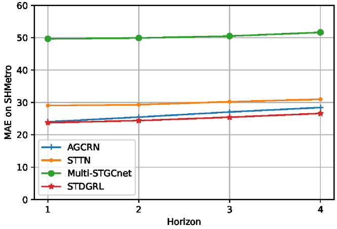
(a) MAE

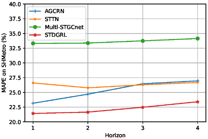
(b) MAPE

Figure 4: Prediction performance at each horizon on the SHMetro dataset.

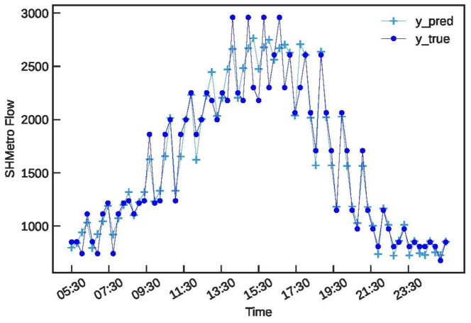
(a) Inflow

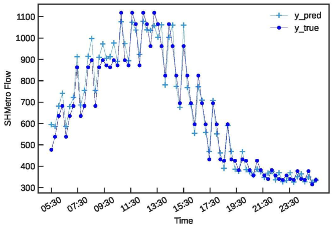
(b) Outflow

Figure 5: Inflow and outflow prediction visualization on the SHMetro dataset.

The Table III to Table VI show the overall prediction performance of our method and 11 comparative methods on the Chongqing, Shanghai, Hangzhou and Beijing Metro datasets. In the prediction interval of the next hour, three evaluation indicators MAE, RMSE, and MAPE are used for evaluation. Our proposed STDGRL method has good performance in both short-term and long-term forecasts, as shown in the Figure 4. With the expansion of the prediction interval, the performance of AGCRN method in MAE and MAPE evaluation indicators gradually deteriorates, and the range of change is larger than that of the STDGRL method, indicating that our method has better performance in the long prediction interval. In addition, compared with STTN and Multi-STGCnet methods, our method has obvious performance advantages in both short-term and long-term prediction intervals. We can see that the results of the classical machine learning-based time series forecasting method are not better than the deep learning-based method such as LSTM, GRU methods, indicating that the modeling of no-linear data dependencies in the spatiotemporal data is crucial when making traffic predictions. In addition, we also find that the performance of the traffic prediction models based on graph neural network proposed in recent years are better than LSTM and GRU methods. The reason is that they can capture the spatio-temporal dependence in spatio-temporal graph data better than the deep learning model. We observe that the performance of AGCRN method is better than other baseline models. It significantly improves experimental results, and this method is second only to our method STDGRL. It indicates that the learned spatial relationship from spatiotemporal data can better reflect its spatial dependence. In addition, we also conduct experiments on three public metro datasets, and the experimental results are shown in Table IV, Table V and Table VI. On the Shanghai Metro dataset, the STDGRL still has significant advantages. Figure 5 shows the inflow and outflow prediction performance at one day in the SHMetro dataset. This dataset contains 288 stations more than other cities stations like Chongqing, Hangzhou. It shows that our proposed method performs well on a small number of stations and also achieves good experimental results on a large number of stations.

TABLE III: Performance comparison of baseline methods on CQMetro dataset.

Model	15min			30min			45min			60min
	MAE	RMSE	MAPE	MAE	RMSE	MAPE	MAE	RMSE	MAPE	MAE	RMSE	MAPE
HA	22.6873	44.4672	1.0492	22.6873	44.4672	1.0492	22.6873	44.4672	1.0492	22.6873	44.4672	1.0492
SVR	23.0547	47.6177	1.2276	23.4774	48.2486	1.2468	24.3611	49.8825	1.2916	25.4671	51.9743	1.3365
LSTM	14.9742	29.9744	0.8541	14.8153	29.3528	0.9047	15.0312	29.7017	0.9033	15.4540	30.0687	1.1451
GRU	14.4919	27.8482	0.8277	14.2734	26.5776	0.8878	14.5248	26.9794	0.9767	15.1376	27.7783	1.3291
T-GCN	21.6926	35.1871	1.6189	23.2144	37.0886	1.9629	25.2631	41.2690	2.0706	27.0057	45.2837	2.4766
DCRNN	15.4474	29.1529	0.8449	16.1849	29.6531	0.9011	17.4521	32.8911	0.9376	18.6397	36.2879	1.0071
STGCN	15.1819	27.3737	0.9369	15.9876	27.9732	1.0453	17.5419	31.0785	1.1385	19.0031	34.5544	1.2687
AGCRN	12.8773	23.5496	0.7516	12.9903	23.0776	0.8022	13.1126	23.4551	0.8241	13.4228	23.8650	0.9641
STTN	14.9288	27.4377	0.8612	14.9991	27.5921	0.8730	15.0118	27.5057	0.8710	15.2668	27.9943	0.9712
Graphwavenet	14.1766	25.1481	0.7942	14.3751	25.1149	0.8532	14.9222	25.9422	0.9627	15.4853	27.0418	1.1322
Multi-STGCnet	18.0469	40.5857	0.8304	17.9263	39.9126	0.8821	17.9012	39.9775	0.8321	17.9893	40.1645	0.8680
STDGRL(ours)	12.5579	22.6911	0.6878	12.6113	22.6256	0.7521	12.6616	22.7524	0.7372	12.8485	23.0310	0.8224
Improvements	+2.48%	+3.65%	+8.48%	+2.92%	+1.96%	+6.25%	+3.44%	+3.00%	+10.54%	+4.28%	+3.49%	+5.26%

TABLE IV: Performance comparison of baseline methods on SHMetro dataset.

Model	15min			30min			45min			60min
	MAE	RMSE	MAPE	MAE	RMSE	MAPE	MAE	RMSE	MAPE	MAE	RMSE	MAPE
HA	76.9445	169.6002	0.9358	76.9445	169.6002	0.9358	76.9445	169.6002	0.9358	76.9445	169.6002	0.9358
SVR	89.4518	230.2805	1.2532	91.0132	233.0358	1.2225	94.6976	239.6837	1.2640	100.0826	249.1291	1.3695
LSTM	48.1613	108.2152	0.6381	53.4732	125.0903	0.6604	57.8482	136.6724	0.6826	64.2742	156.8241	0.7489
GRU	31.2748	65.8625	0.3176	31.6766	67.4298	0.3108	32.5833	71.2581	0.3151	33.7280	74.3567	0.3235
T-GCN	74.6434	124.6865	1.3138	83.4037	147.2772	1.3331	95.1702	176.0193	1.5574	106.0074	202.7877	1.8807
DCRNN	27.9394	54.2426	0.2633	31.9161	63.9539	0.2937	37.2232	79.1991	0.3157	42.0734	93.8128	0.3435
STGCN	28.2697	52.2552	0.3136	31.8696	59.3756	0.3527	36.9222	70.1263	0.4005	42.0439	81.2147	0.4431
AGCRN	24.0087	47.1056	0.2316	25.4590	50.9641	0.2470	27.0434	55.5671	0.2647	28.4134	59.6148	0.2696
STTN	29.0291	56.2013	0.2661	29.2963	57.8522	0.2578	30.2127	60.4864	0.2629	30.9729	60.7344	0.2669
Graphwavenet	26.2299	50.3182	0.2448	28.1380	54.7953	0.2689	30.1868	59.8046	0.2868	32.5230	65.6138	0.3265
Multi-STGCnet	49.6580	128.6207	0.3332	49.9009	128.9203	0.3338	50.4986	129.8213	0.3375	51.6335	131.7302	0.3415
STDGRL(ours)	23.7239	46.8692	0.2143	24.3754	49.2925	0.2166	25.4230	52.9028	0.2248	26.5829	57.3964	0.2341
Improvements	+1.19%	+0.50%	+7.48%	+4.26%	+3.28%	+12.33%	+5.99%	+4.79%	+14.49%	+6.44%	+3.72%	+12.29%

TABLE V: Performance comparison of baseline methods on HZMetro dataset.

Model	15min			30min			45min			60min
	MAE	RMSE	MAPE	MAE	RMSE	MAPE	MAE	RMSE	MAPE	MAE	RMSE	MAPE
HA	71.8148	136.8056	0.6089	71.8148	136.8056	0.6089	71.8148	136.8056	0.6089	71.8148	136.8056	0.6089
SVR	84.8943	170.9875	1.7489	86.6150	173.4301	1.7447	89.1909	177.8438	1.7926	92.4263	183.5363	1.8661
LSTM	27.8706	50.2641	0.2675	28.1602	50.9464	0.2695	28.6903	51.7961	0.2732	29.4597	53.0576	0.3338
GRU	27.2826	48.6847	0.2523	27.7143	49.7454	0.2591	27.9942	50.6825	0.2614	28.6244	51.9195	0.3024
T-GCN	47.3206	69.9398	0.7409	51.0303	78.8955	0.7698	57.6238	91.5450	0.8880	65.0028	103.6740	1.2022
DCRNN	27.1144	49.5158	0.2280	31.2308	58.2314	0.2616	36.9020	70.9692	0.2855	42.7503	85.0528	0.3243
STGCN	28.2432	49.0484	0.3032	32.2267	56.2076	0.3548	37.7572	65.9376	0.4239	44.5799	77.8010	0.6117
AGCRN	23.6154	40.3462	0.2335	24.9422	43.1928	0.2647	25.9514	45.2841	0.2544	27.4004	46.7793	0.3134
STTN	28.1227	48.4724	0.2408	28.8057	49.0463	0.2753	28.6228	49.6005	0.2527	30.6277	52.4030	0.3537
Graphwavenet	25.1968	42.5834	0.2475	26.8730	45.1082	0.2803	29.4834	50.6676	0.2851	31.8565	56.0680	0.3253
Multi-STGCnet	44.4798	92.4560	0.3402	43.7682	92.1209	0.3368	43.8611	92.6602	0.3320	45.1232	94.0267	0.3799
STDGRL(ours)	23.2666	39.5458	0.2091	23.7721	40.4317	0.2141	24.8948	42.8774	0.2230	25.8339	45.1779	0.2570
Improvements	+1.48%	+1.98%	+8.28%	+4.69%	+6.39%	+17.40%	+4.07%	+5.31%	+11.75%	+5.72%	+3.42%	+15.02%

TABLE VI: Performance comparison of baseline methods on BJMetro dataset.

Model	15min			30min			45min			60min
	MAE	RMSE	MAPE	MAE	RMSE	MAPE	MAE	RMSE	MAPE	MAE	RMSE	MAPE
HA	95.7779	207.2597	0.7318	95.7779	207.2597	0.7318	95.7779	207.2597	0.7318	95.7779	207.2597	0.7318
SVR	133.3139	313.8002	2.1439	135.0974	317.4431	2.1201	138.4471	323.1964	2.1260	143.1395	330.3005	2.1365
LSTM	99.2410	243.2237	1.9165	102.5640	245.3053	2.0540	107.7217	248.8519	2.5461	115.4902	257.5999	3.8183
GRU	96.3814	237.3694	1.7907	96.5315	238.4541	1.8164	98.0139	240.9763	2.0611	101.0722	245.6744	3.3837
T-GCN	97.1880	157.4604	1.8642	110.1468	183.8415	2.2288	126.7785	217.8278	3.1665	141.9155	250.9208	4.6435
DCRNN	32.4452	67.2273	0.2861	38.5430	81.8017	0.3725	47.0715	103.1199	0.5501	55.3968	125.2164	0.8658
STGCN	32.1576	62.6209	0.3366	37.8507	71.9395	0.4629	44.9624	84.5158	0.7980	50.8894	96.7363	1.5807
AGCRN	25.1688	47.8686	0.2397	25.3167	47.2164	0.2669	26.2948	48.9524	0.3599	26.9285	50.8812	0.5362
STTN	35.6133	78.4165	0.3647	32.7436	63.3843	0.3284	33.2021	62.4016	0.4469	35.8133	68.6054	0.9178
Graphwavenet	30.0961	54.7262	0.3078	32.2696	59.0870	0.3418	34.8733	64.4616	0.4582	37.7106	70.6784	0.8562
Multi-STGCnet	74.9387	205.3702	0.7335	74.8064	205.1637	0.7601	75.0618	205.4398	0.9342	75.5030	206.6044	1.2342
STDGRL(ours)	21.8468	41.2336	0.2015	22.3419	42.3507	0.2167	22.8053	43.1799	0.2908	22.8942	43.3726	0.4393
Improvements	+13.20%	+13.86%	+15.94%	+11.75%	+10.31%	+18.80%	+13.27%	+11.79%	+19.21%	+14.98%	+14.76%	+18.07%

In summary, the experiment result demonstrates that STDGRL can learn the spatial and temporal relation from the metro spatio-temporal graph of different scales and achieve promising predictions performance.

TABLE VII: Analysis of ablation study on CQMetro dataset.

Model	15min			30min			45min			60min
	MAE	RMSE	MAPE	MAE	RMSE	MAPE	MAE	RMSE	MAPE	MAE	RMSE	MAPE
GCGRU(T-GCN)	21.6926	35.1871	1.6189	23.2144	37.0886	1.9629	25.2631	41.2690	2.0706	27.0057	45.2837	2.4766
STDGRL-NAPL	13.1137	24.0971	0.7766	13.2085	23.5815	0.8447	13.5121	24.0103	0.9089	13.8917	24.6763	1.0789
STDGRL-Transformer	12.7363	23.1410	0.7404	12.7988	22.8028	0.8151	12.8622	22.7317	0.8111	12.9504	22.9711	0.8411
STDGRL-GRU-Transformer	12.8098	22.9895	0.7215	12.8164	22.8653	0.7724	12.9719	23.1255	0.7784	13.0303	23.2679	0.8636

TABLE VIII: Analysis of ablation study on SHMetro dataset.

Model	15min			30min			45min			60min
	MAE	RMSE	MAPE	MAE	RMSE	MAPE	MAE	RMSE	MAPE	MAE	RMSE	MAPE
GCGRU(T-GCN)	74.6434	124.6865	1.3138	83.4037	147.2772	1.3331	95.1702	176.0193	1.5574	106.0074	202.7877	1.8807
STDGRL-Transformer	24.6472	47.9299	0.2297	25.5251	50.9482	0.2358	26.7347	55.5103	0.2474	28.0522	61.0607	0.2565
STDGRL-GRU-Transformer	24.5923	47.8691	0.2191	25.4948	50.5436	0.2219	26.9211	54.8073	0.2336	28.3289	59.8896	0.2431
STDGRL-NAPL	24.5406	48.5099	0.2415	26.2928	53.3123	0.2548	27.7053	56.4908	0.2744	28.9449	59.2060	0.2860

TABLE IX: Analysis of ablation study on HZMetro dataset.

Model	15min			30min			45min			60min
	MAE	RMSE	MAPE	MAE	RMSE	MAPE	MAE	RMSE	MAPE	MAE	RMSE	MAPE
GCGRU(T-GCN)	47.3206	69.9398	0.7409	51.0303	78.8955	0.7698	57.6238	91.5450	0.8880	65.0028	103.6740	1.2022
STDGRL-GRU-Transformer	24.2082	40.6312	0.2244	25.2125	42.4502	0.2430	26.9467	45.9737	0.2595	29.4166	50.9448	0.3488
STDGRL-NAPL	23.9697	41.8146	0.2143	25.6265	44.7244	0.2400	27.0741	47.1538	0.2456	28.8701	49.7926	0.2871
STDGRL-Transformer	23.2615	39.7872	0.2178	24.0419	40.9422	0.2300	24.8309	42.4351	0.2415	26.0904	45.1816	0.2977

TABLE X: Analysis of ablation study on BJMetro dataset.

Model	15min			30min			45min			60min
	MAE	RMSE	MAPE	MAE	RMSE	MAPE	MAE	RMSE	MAPE	MAE	RMSE	MAPE
GCGRU(T-GCN)	97.1880	157.4604	1.8642	110.1468	183.8415	2.2288	126.7785	217.8278	3.1665	141.9155	250.9208	4.6435
STDGRL-NAPL	26.2780	50.5006	0.2732	26.8332	50.8173	0.2990	28.3084	54.1128	0.4353	29.2143	56.2724	0.8812
STDGRL-Transformer	24.0629	44.3345	0.2393	24.6776	45.9240	0.2621	25.6731	48.4556	0.3524	26.0899	49.2110	0.6429
STDGRL-GRU-Transformer	23.9464	43.5017	0.2435	24.7591	45.8199	0.2759	25.9610	48.3604	0.4270	26.1943	48.8126	0.8663

(a) MAE

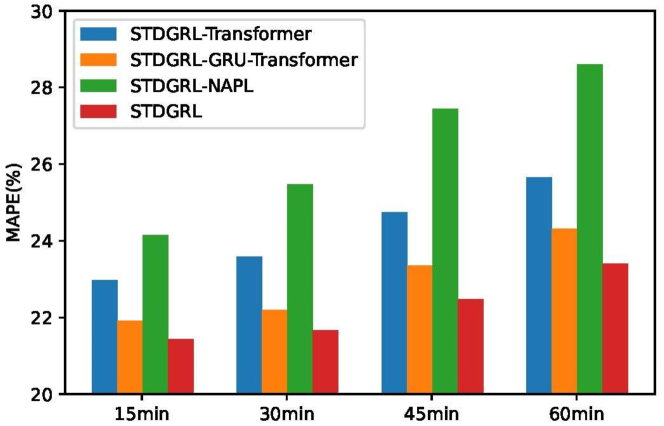
(b) MAPE

Figure 6: Ablation study performance on the SHMetro dataset.

5.3 Ablation Study

We design a comprehensive ablation study to evaluate the performance of STDGRL. The baseline model of our ablation study is GCGRU(T-GCN). This model is a classical traffic forcasting method, which combine GCN and GRU for capturing spatio-temporal dependencies. And we remove the NAPL component from the STDGRL model to construct STDGRL-NAPL. STDGRL-Transformer and STDGRL-GRU-Transformer are the variants of our STDGRL respectively, which remove GRU module, GRU and Transformer module from STDGRL model. The experimental result on the four datasets are illustrated in Table VII, Table VIII, Table IX and Table X. And we also show the ablation study performance on the SHMetro dataset in Figure 6. We can observe that: 1) The results in the Table show that the performance of GCGRU (T-GCN) is not as good as that of the other three comparison models, which may be due to its use of pre-defined graphs and difficulty in capturing complex spatial dependencies between nodes. 2) Compared with the STDGRL model, the performance of the STDGR-NAPL model decreases by a large proportion and is inferior to STDGR-Transformer and STDGR-GRU-Transformer, indicating that it is necessary to capture node-specific traffic patterns in the STDGRL model. 3) After Transformer and GRU modules are removed from the STDGRL model, the performance is lower than that of the STDGRL model, but better than that of the STDGRL-NAPL model, indicating the necessity of using short-term and long-term time series prediction modules in the STDGRL model. And it also demonstrates learning the specific traffic patterns of nodes is more important than learning temporal dependencies.

Overall, our NAPL, DSRL and temporal learning modules jointly boost the prediction performance of the STDGRL model.

6 Conclusion

We proposed STDGRL, a novel spatio-temporal dynamic graph relationship learning model, for predicting multi-step passenger inflow and outflow in urban metro stations. STDGRL can capture the traffic patterns of different metro stations and the dynamic spatial dependencies between metro stations. In addition, STDGRL can capture long-term temporal relationship dependencies for long-term metro flow prediction. We validated our model on real metro datasets in 4 cities and experimental results achieved significant performance improvements over 11 baselines.

In future work, we plan to research the influence of weather, events and POI on the change of metro passenger flow, and the detection and prediction of sudden large passenger flow in metro stations.

References

- [1] Y. Gong, Z. Li, J. Zhang, W. Liu, and Y. Zheng, “Online spatio-temporal crowd flow distribution prediction for complex metro system,” IEEE Transactions on Knowledge and Data Engineering, vol. 34, no. 2, pp. 865–880, 2022.
- [2] Y. Gong, Z. Li, J. Zhang, W. Liu, and J. Yi, “Potential passenger flow prediction: A novel study for urban transportation development,” in Proceedings of the AAAI Conference on Artificial Intelligence, 2020, pp. 4020–4027.
- [3] Q. Cheng, W. Deng, and M. A. Raza, “Analysis of the departure time choices of metro passengers during peak hours,” IET Intelligent Transport Systems, vol. 14, no. 8, pp. 866–872, 2020.
- [4] L. Tang, Y. Zhao, J. Cabrera, J. Ma, and K. L. Tsui, “Forecasting short-term passenger flow: An empirical study on shenzhen metro,” IEEE Transactions on Intelligent Transportation Systems, vol. 20, no. 10, pp. 3613–3622, 2018.
- [5] Y. Liu, Z. Liu, and R. Jia, “Deeppf: A deep learning based architecture for metro passenger flow prediction,” Transportation Research Part C: Emerging Technologies, vol. 101, pp. 18–34, 2019.
- [6] J. Zhang, F. Chen, Z. Cui, Y. Guo, and Y. Zhu, “Deep learning architecture for short-term passenger flow forecasting in urban rail transit,” IEEE Transactions on Intelligent Transportation Systems, vol. 22, no. 11, pp. 7004–7014, 2020.
- [7] P. Chen, X. Fu, and X. Wang, “A graph convolutional stacked bidirectional unidirectional-lstm neural network for metro ridership prediction,” IEEE Transactions on Intelligent Transportation Systems, no. 99, pp. 1–13, 2021.
- [8] J. Ye, J. Zhao, K. Ye, and C. Xu, “Multi-stgcnet: A graph convolution based spatial-temporal framework for subway passenger flow forecasting,” in Proceedings of the 2020 International Joint Conference on Neural Networks, 2020, pp. 1–8.
- [9] X. Ma, J. Zhang, B. Du, C. Ding, and L. Sun, “Parallel architecture of convolutional bi-directional lstm neural networks for network-wide metro ridership prediction,” IEEE Transactions on Intelligent Transportation Systems, vol. 20, no. 6, pp. 2278–2288, 2018.
- [10] J. Ou, J. Sun, Y. Zhu, H. Jin, Y. Liu, F. Zhang, J. Huang, and X. Wang, “Stp-trellisnets: Spatial-temporal parallel trellisnets for metro station passenger flow prediction,” in Proceedings of the 29th ACM International Conference on Information & Knowledge Management, 2020, pp. 1185–1194.
- [11] L. Liu, J. Chen, H. Wu, J. Zhen, G. Li, and L. Lin, “Physical-virtual collaboration modeling for intra-and inter-station metro ridership prediction,” IEEE Transactions on Intelligent Transportation Systems, vol. 23, no. 4, pp. 3377–3391, 2020.
- [12] J. Chen, L. Liu, H. Wu, J. Zhen, G. Li, and L. Lin, “Physical-virtual collaboration graph network for station-level metro ridership prediction,” arXiv preprint arXiv:2001.04889, 2020.
- [13] Q. Chen, X. Song, H. Yamada, and R. Shibasaki, “Learning deep representation from big and heterogeneous data for traffic accident inference,” in Proceedings of the AAAI Conference on Artificial Intelligence, 2016, pp. 338–344.
- [14] K. Jayarajah, A. Tan, and A. Misra, “Understanding the interdependency of land use and mobility for urban planning,” in Proceedings of the 2018 ACM International Joint Conference and 2018 International Symposium on Pervasive and Ubiquitous Computing and Wearable Computers, 2018, pp. 1079–1087.
- [15] J. Zhang, Y. Zheng, and D. Qi, “Deep spatio-temporal residual networks for citywide crowd flows prediction,” in Proceedings of the AAAI Conference on Artificial Intelligence, 2017, pp. 1655–1661.
- [16] J. Zhang, Y. Zheng, D. Qi, R. Li, and X. Yi, “Dnn-based prediction model for spatio-temporal data,” in Proceedings of the 24th ACM SIGSPATIAL International Conference on Advances in Geographic Information Systems, 2016, pp. 92:1–92:4.
- [17] P. Xie, T. Li, J. Liu, S. Du, X. Yang, and J. Zhang, “Urban flow prediction from spatiotemporal data using machine learning: A survey,” Information Fusion, vol. 59, pp. 1–12, 2020.
- [18] B. M. Williams, P. K. Durvasula, and D. E. Brown, “Urban freeway traffic flow prediction: application of seasonal autoregressive integrated moving average and exponential smoothing models,” Transportation Research Record, vol. 1644, no. 1, pp. 132–141, 1998.
- [19] N. Zhang, Y. Zhang, and H. Lu, “Seasonal autoregressive integrated moving average and support vector machine models: prediction of short-term traffic flow on freeways,” Transportation Research Record, vol. 2215, no. 1, pp. 85–92, 2011.
- [20] M. Lippi, M. Bertini, and P. Frasconi, “Short-term traffic flow forecasting: An experimental comparison of time-series analysis and supervised learning,” IEEE Transactions on Intelligent Transportation Systems, vol. 14, no. 2, pp. 871–882, 2013.
- [21] F. G. Habtemichael and M. Cetin, “Short-term traffic flow rate forecasting based on identifying similar traffic patterns,” Transportation Research Part C: Emerging Technologies, vol. 66, pp. 61–78, 2016.
- [22] Z. Zhao, W. Chen, X. Wu, P. C. Chen, and J. Liu, “Lstm network: a deep learning approach for short-term traffic forecast,” IET Intelligent Transport Systems, vol. 11, no. 2, pp. 68–75, 2017.
- [23] W. Jiang and L. Zhang, “Geospatial data to images: A deep-learning framework for traffic forecasting,” Tsinghua Science and Technology, vol. 24, no. 1, pp. 52–64, 2018.
- [24] Y. Wu, H. Tan, L. Qin, B. Ran, and Z. Jiang, “A hybrid deep learning based traffic flow prediction method and its understanding,” Transportation Research Part C: Emerging Technologies, vol. 90, pp. 166–180, 2018.
- [25] Z. Duan, Y. Yang, K. Zhang, Y. Ni, and S. Bajgain, “Improved deep hybrid networks for urban traffic flow prediction using trajectory data,” IEEE Access, vol. 6, pp. 31 820–31 827, 2018.
- [26] J. Zhang, Y. Zheng, J. Sun, and D. Qi, “Flow prediction in spatio-temporal networks based on multitask deep learning,” IEEE Transactions on Knowledge and Data Engineering, vol. 32, no. 3, pp. 468–478, 2019.
- [27] H. Yao, X. Tang, H. Wei, G. Zheng, and Z. Li, “Revisiting spatial-temporal similarity: A deep learning framework for traffic prediction,” in Proceedings of the AAAI Conference on Artificial Intelligence, 2019, pp. 5668–5675.
- [28] J. Bruna, W. Zaremba, A. Szlam, and Y. LeCun, “Spectral networks and deep locally connected networks on graphs,” in Proceedings of the 2nd International Conference on Learning Representations, 2014.
- [29] M. Defferrard, X. Bresson, and P. Vandergheynst, “Convolutional neural networks on graphs with fast localized spectral filtering,” in Advances in Neural Information Processing Systems, 2016, pp. 3837–3845.
- [30] T. N. Kipf and M. Welling, “Semi-supervised classification with graph convolutional networks,” in Proceedings of the 5th International Conference on Learning Representations, 2017.
- [31] W. Jiang and J. Luo, “Graph neural network for traffic forecasting: A survey,” arXiv preprint arXiv:2101.11174, 2021.
- [32] Y. Li, R. Yu, C. Shahabi, and Y. Liu, “Diffusion convolutional recurrent neural network: Data-driven traffic forecasting,” in Proceedings of the 6th International Conference on Learning Representations, 2018.
- [33] B. Yu, H. Yin, and Z. Zhu, “Spatio-temporal graph convolutional networks: a deep learning framework for traffic forecasting,” in Proceedings of the Twenty-Seventh International Joint Conference on Artificial Intelligence, 2018, pp. 3634–3640.
- [34] Z. Wu, S. Pan, F. Chen, G. Long, C. Zhang, and S. Y. Philip, “A comprehensive survey on graph neural networks,” IEEE Transactions on Neural Networks and Learning Systems, vol. 32, no. 1, pp. 4–24, 2020.
- [35] L. Zhao, Y. Song, C. Zhang, Y. Liu, P. Wang, T. Lin, M. Deng, and H. Li, “T-gcn: A temporal graph convolutional network for traffic prediction,” IEEE Transactions on Intelligent Transportation Systems, vol. 21, no. 9, pp. 3848–3858, 2019.
- [36] L. BAI, L. Yao, C. Li, X. Wang, and C. Wang, “Adaptive graph convolutional recurrent network for traffic forecasting,” in Advances in Neural Information Processing Systems, 2020, pp. 17 804–17 815.
- [37] A. Vaswani, N. Shazeer, N. Parmar, J. Uszkoreit, L. Jones, A. N. Gomez, L. Kaiser, and I. Polosukhin, “Attention is all you need,” in Advances in Neural Information Processing Systems, 2017, pp. 5998–6008.
- [38] K. He, X. Zhang, S. Ren, and J. Sun, “Deep residual learning for image recognition,” in Proceedings of the 2016 IEEE Conference on Computer Vision and Pattern Recognition, 2016, pp. 770–778.
- [39] A. Paszke, S. Gross, F. Massa, A. Lerer, J. Bradbury, G. Chanan, T. Killeen, Z. Lin, N. Gimelshein, L. Antiga et al., “Pytorch: An imperative style, high-performance deep learning library,” in Advances in Neural Information Processing Systems, 2019, pp. 8024–8035.
- [40] D. P. Kingma and J. Ba, “Adam: A method for stochastic optimization,” arXiv preprint arXiv:1412.6980, 2014.
- [41] J. Liu and W. Guan, “A summary of traffic flow forecasting methods,” Journal of Highway and Transportation Research and Development, vol. 3, pp. 82–85, 2004.
- [42] A. J. Smola and B. Schölkopf, “A tutorial on support vector regression,” Statistics and Computing, vol. 14, no. 3, pp. 199–222, 2004.
- [43] S. Hochreiter and J. Schmidhuber, “Long short-term memory,” Neural Computation, vol. 9, no. 8, pp. 1735–1780, 1997.
- [44] K. Cho, B. van Merriënboer, D. Bahdanau, and Y. Bengio, “On the properties of neural machine translation: Encoder–decoder approaches,” in Proceedings of SSST-8, Eighth Workshop on Syntax, Semantics and Structure in Statistical Translation, 2014, pp. 103–111.
- [45] Z. Wu, S. Pan, G. Long, J. Jiang, and C. Zhang, “Graph wavenet for deep spatial-temporal graph modeling,” in Proceedings of the Twenty-Eighth International Joint Conference on Artificial Intelligence, 2019, pp. 1907–1913.
- [46] M. Xu, W. Dai, C. Liu, X. Gao, W. Lin, G.-J. Qi, and H. Xiong, “Spatial-temporal transformer networks for traffic flow forecasting,” arXiv preprint arXiv:2001.02908, 2020.