IoT-Scan:
Network Reconnaissance for the Internet of Things

Abstract

Network reconnaissance is a core networking and security procedure aimed at discovering devices and their properties. For IP-based networks, several network reconnaissance tools are available, such as Nmap. For the Internet of Things (IoT), there is currently no similar tool capable of discovering devices across multiple protocols. In this paper, we present IoT-Scan, a universal IoT network reconnaissance tool. IoT-Scan is based on software defined radio (SDR) technology, which allows for a flexible software-based implementation of radio protocols. We present a series of passive, active, multi-channel, and multi-protocol scanning algorithms to speed up the discovery of devices with IoT-Scan. We benchmark the passive scanning algorithms against a theoretical traffic model based on the non-uniform coupon collector problem. We implement the scanning algorithms and compare their performance for four popular IoT protocols: Zigbee, Bluetooth LE, Z-Wave, and LoRa. Through extensive experiments with dozens of IoT devices, we demonstrate that our implementation experiences minimal packet losses and achieves performance near the theoretical benchmark. Using multi-protocol scanning, we further demonstrate a reduction of 70% in the discovery times of Bluetooth and Zigbee devices in the 2.4 GHz band and of LoRa and Z-Wave devices in the 900 MHz band, compared to sequential passive scanning. We make our implementation and data available to the research community to allow independent replication of our results and facilitate further development of the tool.

I Introduction

The Internet of Things (IoT) device market is currently exhibiting exponential growth (among the 29 billion connected devices forecast this year, 18 billion will be related to IoT [1]). These devices run a variety of low-power communication protocols, such as Bluetooth Low Energy (BLE) [2], Zigbee [3], Z-wave [4], and LoRa [5], which support applications in smart homes, smart grid, health care, and environmental monitoring.

The heterogeneity of the IoT ecosystem – and in particular the large number of IoT protocols – represents a major challenge from a network and security monitoring perspective [6, 7]. This heterogeneity makes it hard for network administrators to run network reconnaissance tasks, which aim at discovering wireless IoT devices and their properties. Network reconnaissance is crucial for maintaining an asset inventory, monitoring changes in device behavior, and detecting rogue devices. Since many IoT devices are mobile (e.g., wearables and trackers), network reconnaissance tasks must be run regularly. New laws adopted by regulators, such as the IoT Cybersecurity Improvement Act of 2020 [8] in the US, provide further impetus to the design of effective solutions for IoT network reconnaissance.

The simplest solution for IoT network reconnaissance is to use a monitoring device equipped with a different network card for each protocol. However, even devices operating on the same protocol may be incompatible if they run different versions of the protocol (e.g., normal versus long-range Z-Wave [9]). Using dozens of different USB dongles or network cards for each protocol is prohibitive for practical network security auditing.

Existing software tools for network reconnaissance, such as Nmap [10], focus on devices with IP addresses. Nmap can scan IP/port ranges for an arbitrary number of local or remote hosts and their services. However, this approach is limited to IP-enabled devices only, and yet many popular IoT protocols, including BLE, Zigbee, Z-Wave, and LoRa do not support IP addressing. While there is currently an effort by several vendors to create a unified, IP-based IoT protocol, called Matter [11], its level of adoption and backward-compatibility with legacy devices remain uncertain.

To address this current gap, we propose IoT-Scan, an extensible, multi-protocol IoT network reconnaissance tool for enumerating IoT devices. IoT-Scan runs both on the 900 MHz and 2.4 GHz bands and currently supports four popular IoT protocols: Zigbee, BLE, LoRa, and Z-Wave. Remarkably, IoT-Scan runs on a single piece of hardware, namely a software-defined radio (SDR) [12].

IoT-Scan leverages software-defined implementation of IoT communication protocol stacks, mostly under the GNU Radio ecosystem [13, 14]. This approach reduces the amount of hardware needed to address the growing number of IoT protocols. This further allows for future expansion into new protocol versions, thus eliminating the need of purchasing or upgrading protocol-specific hardware [15].

A key challenge faced in the design of IoT-Scan lies in minimizing the discovery time of devices. A simple approach (which we refer to as a sequential algorithm) is to scan devices in a round robin fashion across each individual protocol, and in turn across each individual channel within each protocol. However, this approach does not scale. Consider, for instance, that Zigbee devices can communicate over 16 different channels.

To address the above, we propose, implement, and benchmark several scanning algorithms to speed up the discovery of IoT devices. These algorithms, of increasing sophistication, can listen in parallel across different channels and different protocols. To achieve this, our work takes on the challenge of integrating single-protocol physical layer implementations of IoT protocols for SDRs to perform parallel scanning across channels and protocols, under the constraints of limited instantaneous bandwidth (i.e., the range of frequencies to which the SDR is tuned at a given point in time). Indeed, the channel spread defined by most protocols operating in the 2.4 GHz band is wider than the typical instantaneous bandwidth of an SDR, i.e., it is typically not possible to monitor the entire spectrum of a protocol simultaneously with one monitoring device.

Another challenge is that some IoT devices transmit sparingly (e.g., due to energy savings considerations), and enumerating devices passively on the wireless channel can result in long discovery times. To speed up discovery of such devices, we propose active scanning algorithms that send probe messages to discover which channels are actively used by devices of a given protocol, and skip channels on which no communication is taking place. We demonstrate these algorithms for Zigbee devices.

Another important consideration is evaluating the efficiency of the scanning algorithm implementation on the SDR, namely whether devices are indeed discovered as fast as possible and no packet loss is incurred due to imperfect SDR implementation. We achieve this by establishing a connection between our network scanning problem and the non-uniform coupon collector problem [16, 17], whereby each transmission by a specific device corresponds to a coupon of a certain type and the objective is to collect a coupon of each type as fast as possible. The non-uniformity of the problem stems from the different rates at which different devices transmit packets. Under appropriate statistical assumptions, we can analyze this problem and numerically compute the expectation of the order statistics of the discovery times (i.e., the average time to discover $n$ out of $N$ devices, for any $n=1,2,\dots,N$). For the cases of Zigbee and BLE, we show that the discovery times, as measured through several repeated experiments, closely align with these theoretical benchmarks.

Our main contributions are thus as follows:

• We introduce IoT-Scan, a universal tool for IoT network reconnaissance. IoT-Scan consists both of a collection of efficient and practical IoT scanning algorithms and of their implementations using a single commercial off-the-shelf software-defined radio device, namely a USRP B200 SDR [18].

• We validate the performance of the algorithms through extensive experiments on a large collection of devices. We demonstrate multi-protocol, multi-channel scanning both on the 2.4 GHz band for Zigbee and BLE, and on the 900 MHz band for LoRa and Z-Wave.

• We propose new active scanning algorithms and show an implementation for Zigbee, which cuts down the discovery time by 87%, from 365 s to 46 s, compared to a sequential scanning algorithm.

• We develop a theoretical benchmark based on the non-uniform coupon collector problem, and show that passive scan algorithms for Zigbee and BLE achieves performance near that benchmark

• We discuss implementation challenges and parameter optimizations as they relate to scanning performance.

The rest of this paper is structured as follows. Section II discusses related work. Section III presents the scanning methods and algorithms forming the core of IoT-Scan. Section IV discusses performance metrics for the algorithms, as well as a theoretical model for benchmarking device discovery. Section V provides background on each of the IoT protocols covered in this paper, and elaborates on how IoT-Scan discovers addresses of devices in each case. Section VI presents our experiments, including implementation aspects, experimental setup, and results. Section VII concludes our findings, discusses ethical issues, and presents an outlook on future work.

II Related Work

This section presents related work. Most existing work focuses on protocol-specific techniques. In contrast our work introduces several cross-protocol algorithms for IoT scanning, and further benchmarks their performance both theoretically and experimentally.

Heinrich et al. presents BTLEmap [19], a BLE-focused device enumeration and service discovery tool inspired by traditional network scanning tools like Nmap [10]. Aside from an extended message dissector based on both the BLE specification as well as previous reverse-engineering work on Apple-specific message types, BTLEmap shares similarities to tools available in the Linux Bluetooth stack. While BTLEMap supports both Apple’s Core Bluetooth protocol stack and external scanner sources, it is limited to Bluetooth LE by design and does not aim to support multiple protocols. In contrast, IoT-Scan is not tied to a particular vendor as a host device, and supports multiple protocols simultaneously, with one radio source.

Tournier et al. propose IoTMap [20], which models inter-connected IoT networks using various protocols, and deduces network characteristics on multiple layers of the respective protocol stacks. IoTMap has a strong focus on modeling network layers in a cross-protocol environment, as well as identification of application behavior and network graphs across protocols. However, IoTMap requires dedicated radios for each protocol in order to operate, whereas IoT-Scan achieves device detection across multiple protocols with a single software-defined radio transceiver.

In a preliminary poster [21], we introduced a precursor to IoT-Scan that showcased scanning of BLE and Zigbee devices with an SDR platform. IoT-Scan encompasses additional protocols, namely LoRa and Z-Wave. Furthermore, our work introduces novel scanning algorithms and conducts extensive evaluation of these algorithms, both theoretically and empirically with dozens of IoT devices. In contrast, our preliminary work did not present scanning algorithms and had no evaluation contents (either theoretical or empirical).

Bak et al. [22] optimize BLE advertising scan (i.e., device discovery) by using three identical BLE dongles. This approach is not scalable since it requires a new hardware receiver for each new channel, and equally does not scale beyond the BLE protocol. In contrast, our SDR-based approach uses the same SDR hardware to receive multiple protocols.

Kilgour [23] presents a multi-channel BLE capture and analysis tool implemented on a field programmable gate array (FPGA). This multi-channel BLE tool allows receiving data from multiple channels in parallel. However, the focus is on BLE PHY receiver implementation and related signal processing rather than actual scanning and enumeration of devices. Kilgour’s work discusses FPGA extensions for the USRP N210 platform which in theory allow for a large number of Bluetooth LE channels to be received in parallel. However, no practical validation is performed to demonstrate this configuration. In contrast, our work extends beyond Bluetooth LE, and crucially performs practical device enumeration scans to quantify scanning performance.

Active scan is a known device discovery technique used in Wi-Fi [24]. Thus, Park et al. describe a Wi-Fi active scan technique performed using BLE radio using cross-protocol interference [25]. The active scan algorithms in IoT-Scan are motivated by similar ideas, but require judicious use of protocol-specific mechanisms (i.e., sending beacon request packets in Zigbee).

Hall et al. [26] describe a tool, called EZ-Wave that can discover Z-Wave devices passively and actively. The EZ-Wave tool actively scans a Z-Wave device by sending a “probe” packet with acknowledgement request flag set. In the older version S0 of the Z-Wave protocol, it was compulsory for a Z-Wave device to reply with acknowledgements to such packets. By getting this acknowledgement back, the EZ-Wave tool learns about a device’s presence. However, the EZ-Wave tool only supports older versions of Z-Wave protocol. In the new version (S2) of the Z-Wave protocol, acknowledgements are not compulsory and this is not a reliable active scan mechanism. The old Z-Wave protocol uses only the R1 (9.6 kbps) and R2 (40 kbps) physical layers. Our work adds R3 (100 kbps PHY) as well as multi-protocol capabilities. The R1, R2, and R3 rates are defined in [4, Table 7-2].

Choong [27] implement a multi-channel IEEE 802.15.4 receiver using a USRP2 software-defined radio. The USRP2 has a maximum sample window of 25 MHz and maximum Ethernet backbone (radio to PC communication) transfer rate of 30 MS/s. This limits the multi-channel receiver to a maximum of five (consecutive) Zigbee channels. Choong describes a channelization method similar to the receive chain used in this work (see Section 2) that extracts multiple channels from a wider raw signal stream. However, Choong’s work focuses on the performance impact of the SDR host computer, and is a Zigbee-specific implementation, whereas our work focuses on device enumeration in a multi-channel as well as multi-protocol context.

Our Zigbee, BLE, and Z-Wave GNU Radio receiver implementations are based on scapy-radio [14] flowgraphs. Our LoRa GNU Radio receiver flowgraph is based on a work by Tapparel et al. [5]. A similar multi-channel LoRa receiver was implemented by Robyns in [28]. In order to support multi-radio, multi-channel capabilities, IoT-Scan implements several changes to these GNU Radio receiver implementations. In general, these changes pertain to the signal path between the SDR source and the receive chains for individual channels and protocols (i.e., frequency translation, filtering, and resampling, see Section VI-A). Additionally, our LoRa receiver can listen to LoRa packets promiscuously.

III Scanning Algorithms

In this section, we introduce SDR-based scanning algorithms that form the core of IoT-Scan. Alongside, we introduce several auxiliary helper functions. The notion of channel in this section refers to a 3-tuple containing the center frequency of the channel, the channel bandwidth (i.e., a range of frequencies delineated by the lower and upper frequencies of the channel), and the protocol type. The concept of instantaneous bandwidth refers to the range of frequencies captured by the SDR at any given point of time. The center frequency corresponds to the frequency at the middle of the range.

III-A Single-channel methods

$\triangleright$ Receive packets on channel $ch$ for duration $dwell\_time$ and return a list of discovered devices

1 $t_{start}\leftarrow$time() $\triangleright$ Store current time

2 $device\_list\leftarrow\{\}$ $\triangleright$ Initialize device list

3 while time()$-t_{start}\leq dwell\_time$ do

4       Listen on channel $ch$

5       Get packet and extract address $dev\_addr$

6       $device\_list=device\_list\cup dev\_addr$

7      

8 end while

return $device\_list$

Algorithm 1 Listen($ch,dwell\_time$)

The key building block to any of the following scanning algorithms is the function Listen() (Algorithm 1). It takes two input parameters, namely a channel $ch$ (defined by a center frequency, bandwidth and protocol) and a time period $dwell\_time$ after which the procedure terminates listening to channel $ch$. During execution of this procedure, the SDR decodes any packet received on the channel, and extracts address information $dev\_addr$ that identifies a device (line 1). Note that some packets may have no address information, in which case $dev\_addr$ is an empty set. Next, the device address is added to the list of discovered devices $device\_list$ (line 1). By definition, if $dev\_addr$ already appears in $device\_list$, then the union operation does not change the contents of the list. Upon the expiration of the channel dwelling time, the procedure returns the list of discovered devices.

$\triangleright$ Enumerate devices by repeatedly listening for duration $dwell\_time$ on each channel in $ch\_list$ and stop after $scan\_time$

1

2

3$t_{start}\leftarrow$time() $\triangleright$ Store current time

4 $device\_list\leftarrow\{\}$ $\triangleright$ Initialize device list

5 $i\leftarrow 0$ $\triangleright$ Set channel counter to zero

6 while time()$-t_{start}\leq scan\_time$ do

       $\triangleright$ $ch\_list(i)$ is the $i$-th element in $ch\_list$

7      

8      $new\_dev\leftarrow$ Listen($ch\_list(i),dwell\_time$)

9       $device\_list=device\_list\cup new\_dev$

10       $i\leftarrow(i+1)$ mod $|ch\_list|$

11      

12 end while

13

return $device\_list$

Algorithm 2 Passive_Scan($ch\_list,\newline dwell\_time,$ $scan\_time$)

Algorithm 2 presents a simple sequential scanning procedure Passive_Scan that can be used in conjunction with any IoT protocol. This algorithm represents a baseline against which the performance of more advanced algorithms can be compared. The algorithm invokes the Listen procedure in a round-robin fashion on each channel of a given channel list $ch\_list$, which is provided as an input to the procedure. The total scan time is set by the $scan\_time$ input parameter. Note that generally $scan\_time\gg dwell\_time$, and hence each channel is visited several times during the scan. The algorithm returns the list of discovered devices.

$\triangleright$ Actively probe each channel $ch$ from the channel list $ch\_list$ for duration of $dwell\_time$.

1 $active\_channels\leftarrow\{\}$

2 $device\_list\leftarrow\{\}$

3 for $ch\in ch\_list$ do

4       Send probe on channel $ch$ $\triangleright$ Trigger responses

5       $new\_dev\leftarrow$ Listen($ch,dwell\_time$)

6       if $new\_dev\neq\{\}$ then

7             $device\_list\leftarrow device\_list\cup new\_dev$ $\triangleright$ Add found devices

8             $active\_channels\leftarrow active\_channels\cup ch$ $\triangleright$ Add channel to active channel list

9            

10       end if

11      

12 end for

return $active\_channels,device\_list$

Algorithm 3 Probe_Channels($ch\_list,dwell\_time$)

$\triangleright$ Enumerate devices by first identifying the list of $active\_channels$ in $ch\_list$ and then performing passive scanning only on those $active\_channels$

1

2$device\_list\leftarrow\{\}$ $\triangleright$ Initialize list of found devices

3 $active\_channels\leftarrow\{\}$ $\triangleright$ Initialize list of busy channels

4 $t_{start}\leftarrow$time() $\triangleright$ store current time

5

$\triangleright$ Phase 1: Scan active devices

6 $active\_channels,device\_list\leftarrow\textbf{Probe\_Channels}(ch\_list,dwell\_time)$

7

$\triangleright$ Phase 2: Passive-scan known active channels for the remaining time

8 $t_{scan}\leftarrow scan\_time-(\textnormal{time()}-t_{start})$ $\triangleright$ Compute remaining scanning time

9 $new\_dev\leftarrow\textbf{Passive\_Scan}(active\_channels,dwell\_time,t_{scan})$ $\triangleright$ Run passive scan on active channels

10 $device\_list\leftarrow device\_list\cup new\_dev$ $\triangleright$ Add devices found during passive scanning

return $device\_list$

Algorithm 4 Active_Scan($ch\_list,dwell\_time,scan\_time$)

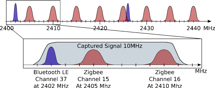
Figure 1: Find_Channels_In_Range() (Algorithm 5) starts at the lowest channel in the provided list and returns all channels that are in range of the SDR hardware based on the provided instantaneous bandwidth parameter.

Sequential passive scanning can be slow, especially if an IoT protocol supports many channels, but only a few channels are used. In order to speed up device discovery, Algorithm 4, which we refer to as Active_Scan, implements a two-phase approach. During the first phase (line 4), it invokes a helper function Probe_Channels (Algorithm 3), which sends a probe packet on each channel $ch$ in the provided $channel\_list$ and waits for a response. If one or more devices respond, then channel $ch$ is added to the $active\_channels$ list. During the second phase (lines 4–4), Algorithm 4 performs passive scanning only on channels appearing in the $active\_channels$ list for the remaining scan time. Algorithm 4 is especially useful for protocols such as Zigbee, which defines 16 different channels, not all of which may be in use. For Zigbee, IoT-Scan implements the probe packet using a beacon request frame, to which Zigbee coordinators and routers respond with a beacon frame (see also Section V).

III-B Multi-channel methods

The subsequent algorithms expand from single channel scanning to handling multiple channels and multiple protocols, at the same time.

1

$\triangleright$ Identify all channels in $ch\_list$ (ordered by ascending frequency) that can fit in the instantaneous $bandwidth$, starting from the first element $ch\_list(0).$

2 $ch\_range\!\leftarrow\!\{\!$all $ch$ in $ch\_list$ such that $(ch._{freq}+ch._{bw}/2)-(ch\_list(0)._{freq}-ch\_list(0)._{bw}/2)\leq bandwidth\!$}

return $ch\_range$

Algorithm 5 Find_Channels_In_Range($ch\_list,bandwidth$)

Prior to discussing multi-channel and multi-protocol scanning algorithms, we need a method of grouping channels within the range of the instantaneous bandwidth of the SDR. Find_Channels_In_Range() (Algorithm 5) identifies all channels in an input channel list (ordered by ascending frequency) by selecting all channels that fit the instantaneous bandwidth under consideration of their respective center frequencies and channel bandwidths, see Fig. 1. For a channel to be considered in range, the entire bandwidth of the signal must be contained in the captured instantaneous bandwidth of the SDR (see line 5 of Algorithm 5).

In practice, the center frequency of each group of channels is set such that the first channel from the channel list (i.e., the one with the lowest frequency) is at the far left end of the instantaneous bandwidth. If none of the other channels’ bandwidths overlap with the current instantaneous bandwidth, the function will return the first element of the input channel list, i.e., it will default to single-channel selection.

1

$\triangleright$ Scan in parallel all channels in $ch\_range$ for a duration $dwell\_time$. Note that all channels are assumed to be within the instantaneous bandwidth of the SDR, e.g. as produced by Find_Channels_In_Range()

2

3do in parallel

4       $new\_dev\leftarrow\{$Listen$(ch,dwell\_time)$ for all $ch$ in $ch\_range$}

5       $device\_list\leftarrow device\_list\,\cup new\_dev$

6      

7 end parallel

8

return $device\_list$

Algorithm 6 Listen_In_Parallel($ch\_range,dwell\_time$)

We further define a helper function Listen_In_Parallel() (Algorithm 6) which simultaneously listens to multiple channels by calling Listen() (Algorithm 1) on all provided channels. Note that implementing this algorithm requires extracting multiple signal streams by frequency-shifting, filtering, and down-conversion or resampling the incoming signal relative to its center frequency and the parameters of the channel. This procedure is called channelization. The implementation aspects of this procedure are described in Section VI-A.

$\triangleright$ This algorithm enumerates devices by scanning as many channels as can fit in the instantaneous bandwidth of $bandwidth$ for a duration $dwell\_time$ in each iteration.

1 $ch\_unscanned\leftarrow ch\_list$ $\triangleright$ All channels in the list are unscanned

2 $ch\_groups\leftarrow\{\}$ $\triangleright$ Initialize list of channel groups

3 while $ch\_unscanned\neq\{\}$ do

       $\triangleright$ Find channels that can be scanned simultaneously as they fit the instantaneous $bandwidth$.

4       $ch\_range\leftarrow$ Find_Channels_In_Range(ch_unscanned, bandwidth)

5      $\triangleright$ Scan channels that fit in instantaneous bandwidth BW around center freq. $ch\_groups\leftarrow ch\_groups\cup\{ch\_range\}$ $\triangleright$ Add this group to the list of channel groups

6       $ch\_unscanned\leftarrow ch\_unscanned\setminus ch\_range$ $\triangleright$ Remove channels from unscanned list

7 end while

8$t_{start}\leftarrow$time() $\triangleright$ Store current time

9 $device\_list\leftarrow\{\}$ $\triangleright$ Initialize list of found devices

10 $i\leftarrow 0$ $\triangleright$ Set channel counter to zero

11 while time()$-t_{start}\leq scan\_time$ do

       $\triangleright$ Scan all channels of the i’th channel group in parallel

12       $new\_dev\leftarrow$ Listen_In_Parallel(ch_group(i), dwell_time)

       $\triangleright$ Remove scanned channels from unscanned channel list

13       $device\_list\leftarrow device\_list\,\cup new\_dev$ $i\leftarrow(i+1)$ mod $|ch\_groups|$

14 end while

return $device\_list$

Algorithm 7 Multiprotocol_Scan($ch\_list,dwell\_time,scan\_time,bandwidth$)

Algorithm 7 describes a parallel multi-protocol scan that can be used with any number of IoT protocols. Based on a list of channels to consider (ordered by ascending frequencies), the algorithm starts at the lowest frequency and determines all channels within range of the first channel by calling Find_Channels_In_Range() (Algorithm 5). It subsequently listens to those channels by invoking Listen_In_Parallel() (Algorithm 6). Note that if only one channel is in range at given step of the while loop (line 12), then the algorithm’s behavior becomes identical to Passive_Scan() (Algorithm 2).

Each such channel hop is scanned for the defined channel $dwell\_time$. Once all unscanned channels are exhausted, the algorithm restarts from the lowest channel until the desired $scan\_time$ has elapsed. Note that the total $scan\_time$ is typically much greater than the channel $dwell\_time$. Depending on the frequency allocation of the protocols involved, the multi-protocol scan algorithm can significantly speed up IoT device discovery process by receiving multiple protocols simultaneously, as demonstrated in Section VI-C.

$\triangleright$ Enumerate devices by first identifying list of $busy\_channels$ from $ch\_probe\_list$ and then performing multi-protocol scanning only on those active channels and on other channels provided in $ch\_list$.

1 $device\_list\leftarrow\{\}$ $\triangleright$ Initialize list of found devices

2 $active\_channels=\{\}$ $\triangleright$ Initialize list of busy channels

3 $t_{start}\leftarrow$ time() $\triangleright$ Store current time

4

$\triangleright$ Probe all channels in $ch\_probe\_list$ to identify active channels

5 $active\_channels,device\_list\leftarrow$ Probe_Channels($ch\_probe\_list,dwell\_time$)

6

7 $t_{scan}\leftarrow scan\_time-(\textnormal{time()}-t_{start})$ $\triangleright$ Compute remaining scanning time

$\triangleright$ Merge successfully probed channels with regular channels and sort by ascending frequency

8 $active\_channels\leftarrow\textnormal{sort}(active\_channels\cup ch\_list)$

$\triangleright$ Run passive scan on all active channels for the remaining time $t_{scan}$

9 $new\_dev\leftarrow$ Multiprotocol_Scan($active\_channels,dwell\_time,t_{scan},bandwidth$)

10 $device\_list\leftarrow device\_list\cup new\_dev$ $\triangleright$ Add devices found during passive scanning

return $device\_list$

Algorithm 8 Active_Multiprotocol_Scan($ch\_list,ch\_probe\_list,dwell\_time,scan\_time,bandwidth$)

Finally, Active_Multiprotocol_Scan() (Algorithm 8) is a combination of the aforementioned active scanning and multi-protocol scanning capabilities. It is useful for scanning multiple protocols, some actively and some passively (such as a combination of Zigbee and BLE). Note that Algorithm 8 receives two lists of channels: $ch\_probe\_list$ and $ch\_list$. Active channels (e.g., Zigbee channels) are only sought among channels in the $ch\_probe\_list$. This step is skipped for channels (e.g., BLE channels) in the $ch\_list$.

IV Performance Metrics and Analysis

In this section, we define metrics to benchmark the various algorithms. We further formalize IoT device discovery as a variation of the non-uniform (weighted) coupon collector problem [16, 17]. Under appropriate statistical assumptions, the coupon collection time can be computed numerically and serve as a baseline against which the performance of the algorithms can be compared.

IV-A Metrics

Our main metric is the discovery time of IoT devices, which we aim to minimize. Assume there are $N$ devices in total, with corresponding discovery times $T_{1},T_{2},\ldots,T_{N}$. We are interested in characterizing the order statistics of these random variables, i.e., the time elapsing till one device is discovered, which is denoted $X_{1:N}$, then till two devices are discovered, which is denoted $X_{2:N}$, and so on, till all devices are discovered, which is denoted $X_{N:N}$. We thus have

$$X_{1:N} = \min(T_{1},T_{2},\dots,T_{N}),$$ (1)

$$X_{2:N} = \min(\{T_{1},T_{2},\dots,T_{N}\}\setminus X_{1:N}),$$ (2)

$$\dots$$

$$X_{N:N} = \max(T_{1},T_{2},\dots,T_{N}).$$ (3)

In our experiments, we estimate the expectation of the $n$-th order statistics $E[X_{n:N}]$, for $n=1,2,\dots,N$. To obtain these estimates, we run each scanning algorithm $M$ times and denote by $x_{n:N}^{(m)}$ the time till $n$ devices are discovered at the $m$-th iteration, where $m=1,2,\dots,M$. We then compute the sample mean for the $n$-th order statistics as follows:

$$\mathrm{bar}{x}_{n:N}=\frac{\sum_{m=1}^{M}x_{n:N}^{(m)}}{M}.$$ (4)

We also provide $(1-\alpha)100\%$ confidence intervals for our estimates

$$[\mathrm{bar}{x}_{n:N}-e_{n:N},\mathrm{bar}{x}_{n:N}+e_{n:N}],$$ (5)

based on computing the sample standard deviation $s_{n:N}$ and the confidence interval parameter $e_{n:N}$ as follows:

$$s_{n:N} = \sqrt{\frac{1}{M-1}\sum_{m=1}^{M}(x_{n:N}^{(m)}-\mathrm{bar}{x}_{n:N})^{2}},$$ (6)

$$e_{n:N} = t_{\alpha/2,M-1}\times\frac{s_{n:N}}{\sqrt{M}},$$ (7)

with $t_{\alpha/2,M-1}$ denoting the $1-\alpha/2$ quantile of the $t$-distribution with $M-1$ degrees of freedom [29]. In our experiments, described in Section VI, we run $M=10$ independent iterations for each algorithm and consider 95% confidence intervals (i.e., $\alpha=0.05$), hence $t_{\alpha/2,M-1}=2.262$ [29, Table 1].

IV-B Theoretical Model

We next propose a theoretical model to estimate the expectations of order statistics of the discovery time, under appropriate statistical assumption. The analysis further assumes an idealized channel environment where no packet loss occurs (in practice such losses could occur due to imperfect receiver implementation or interference). In Section VI-C, we show that the performance of the scanning algorithms approaches that predicted by the theoretical model, which demonstrates the efficiency of the algorithms.

1)   Statistical assumptions

To model device enumeration, we need statistics of the inter-arrival times of packets generated by each device. For the sake of analytical tractability, we assume that devices transmit in a memoryless fashion, i.e., the inter-arrival times of their packets follow an exponential distribution. Note that the mean and standard deviation of an exponential random variable are equal. Hence, we expect that this model can provide a reasonable approximation, if for each device $i$, its mean inter-arrival time $\mu_{i}$ and standard deviation of inter-arrival times $\sigma_{i}$ are roughly equal.

To check this assumption, we collected statistics of the inter-arrival times of packets of the Bluetooth and Zigbee devices listed in Table I below. Specifically, for each device $i$, we measure the times of packet arrivals with $K+1$ timestamps. We then calculate the $K$ inter-arrival times $\tau_{i,k}=t_{i,k+1}-t_{i,k}$, where $k=1,2,\dots,K$. Based on this data, we obtain estimates of the expectation for each device $i$

$$\mu_{i}=\frac{1}{K}\sum_{k=1}^{K}\tau_{i,k},$$ (8)

as well as the standard deviation

$$\sigma_{i}=\sqrt{\frac{1}{K}\sum_{k=1}^{K}(\tau_{i,k}-\mu_{i})^{2}}.$$ (9)

Table I indicates that indeed for all tested BLE devices $\mu_{i}\approx\sigma_{i}$, while this also holds for many, though not all Zigbee devices.

2)   Analysis of order statistics

Enumerating devices shares similarities with the non-uniform coupon collector’s problem [16], albeit with certain modifications.

The coupon collector’s problem assumes a probability distribution in which each draw results in a coupon (i.e., a discovered device). This cannot be applied directly to a scenario in which devices’ transmission characteristics may result in null coupons, i.e., a scan iteration in which no new device is discovered. Anceaume et al. [17] provide a method of calculating the expectation of the non-uniform coupon collector problem which accounts for a null coupon. Define the probability vector $\boldsymbol{p}$ in which $p_{0}$ is the probability of no device transmitting, and $p_{i}$ is the probability of device $i$ transmitting, $i=1,2,\dots,N$. The expectation for the $n$-th order statistics $X_{n,N}$ (i.e., the time to to discover $n$ out of $N$ devices) is then given by

$$\mathbb{E}[X_{n:N}(\boldsymbol{p})]\! = \!\sum_{h=0}^{n-1}R_{N,n,h}\!\sum_{J\in S_{h,N}}\!\frac{1}{1-p_{0}-P_{J}}$$ (10)

with

$$R_{N,n,h} = (-1)^{n-1-h}{N-h-1\choose N-n}.$$ (11)

Here, $S_{h,N}$ denotes all $N\choose h$ subsets containing exactly $h$ devices. Denote by $J$ any subset of $S_{h,N}$ that contains exactly $h$ devices. Then, $P_{J}=\sum_{j\in J}p_{j}$ is the summation of the transmission probabilities of all devices belonging to $J$. Note that the second summation term in Eq. (10) works out to a summation over all possible subsets $J$ of cardinality $h$.

Assuming all $N$ devices send packets in an i.i.d. memoryless fashion as discussed above, the device traffic can be modeled as $N$ independent Poisson processes with rate $\lambda_{i}=1/\mu_{i}$. The combined influx of packets from all the devices then follows a Poisson process with rate $\lambda=\sum_{i=1}^{N}\lambda_{i}$.

By selecting a small interval $\Delta t$ such that either zero or one packet arrives during any interval $\Delta t$, we can use Eq. (10) to compute the expectation of the order statistics of the discovery time of devices. Let $Z$ be a Poisson random variable with mean $\lambda\Delta t$ that counts the number of packets arriving from all devices during a time interval $\Delta t$. We have

$$\Pr(Z=0) = e^{-\lambda\Delta t},$$ (12)

$$\Pr(Z=1) = (\lambda\Delta t)e^{-\lambda\Delta t},$$ (13)

$$\Pr(Z\geq 2) = 1-Pr(Z=0)-Pr(Z=1).$$ (14)

In order to determine a suitable $\Delta t$, we select it such that $Pr(Z\!\geq\!2)$ becomes negligible, as discussed in Section VI-C.

If all devices transmit on one channel that is continuously monitored, the probability $p_{i}$ that device $i$ transmits during an interval $\Delta t$ is then

$$p_{i}=(\lambda_{i}\Delta t)e^{-\lambda_{i}\Delta t}\approx\lambda_{i}\Delta t.$$ (15)

Note that if all devices are randomly distributed on any of $C$ available channels, a randomly channel-hopping radio scanner would receive a transmission from device $i$ with probability $p_{i}/C$. This can also be used as an approximation when the scanner visits channels in a round-robin rather than in a random fashion.

V Protocol Device Enumeration

In the previous sections, the concepts of “listening to a channel” and “extracting device addresses” were presented in a generic way (see Algorithm 1). We now discuss these aspects in detail for all the IoT protocols implemented in IoT-Scan. This section gives an overview of implementation-specific considerations for protocols covered in this work.

V-A Zigbee

Zigbee is a network and application layer protocol which uses the IEEE 802.15.4 physical layer specification [3]. It is widely used in home and commercial building automation applications such as lighting, climate, and access control [30]. Zigbee operates on 16 channels on the 2.4GHz ISM band. Each channel is 2 MHz wide and centered at $f_{c}=2405+5(k-11)$ MHz for channels $k=11...26$ [3, p. 387].

Zigbee defines three types of devices: coordinators, routers, and end-devices, each of which behave differently on the network. End-devices do not route traffic, and are typically mobile and battery-powered, i.e. energy-constrained. As a result, end devices are frequently sleeping, i.e., remain inactive in order to save power. Routers route traffic, receive and store messages for their children (i.e., end devices that they route traffic from and to), and communicate with new nodes requesting to join the network. Therefore, routers cannot sleep and are typically mains-powered devices. A Zigbee coordinator is a special router which, in addition to all of the router capabilities, also forms a network. Before creating a network, Zigbee coordinators scan available channels to select a good, i.e. low interference, channel for the network.

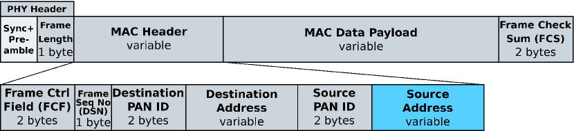
Figure 2: Zigbee medium access control (MAC) layer frame structure [30].

Address Information. IoT-Scan enumerates Zigbee devices by both their short (16 bits) and extended (64 bits) address (whichever of those address types is present in a given packet), ensuring no device is counted double despite these two address formats. While short addresses are unique within a network, extended addresses are typically assigned by the manufacturer in a globally unique way. Some Zigbee packet types will use short and some will use a long address. Both addresses can be parsed from the “Source Address” variable-length field in Figure 2. Note that the PAN ID (personal area network identifier), shown in the same figure, is a network identifier. While we do not use it in our scanning, it could be useful to differentiate between two devices with the same short address but on different networks.

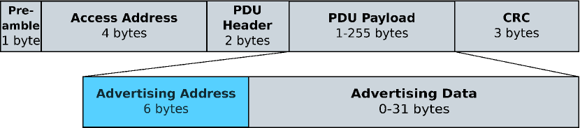
Figure 3: The BLE advertising packet format (top) and the Advertising Channel PDU Header (bottom) for common advertising messages (PDU Types ADV_IND, ADV_NONCONN_IND, ADV_SCAN_IND) [2, p. 2562, 2567].

Implementation. IoT-Scan implements both passive and active scans for Zigbee. A passive scan listens on each channel for a certain amount of time (i.e., the channel dwell time in Algorithm 1) repeatedly until the total scan time expires. With active scanning, channels with network activity are discovered by sending beacon requests on each channel (Algorithm 3). Receiving a beacon frame in response to a beacon request indicates that there is a network on the current channel (note that generally only coordinators and routers reply to beacon requests, end-devices do not). Subsequent passive scanning rounds can then be limited to these active channels (line 4 in Algorithm 4), in order to detect any further devices that did not respond to active scanning (i.e., end-devices).

V-B Bluetooth Low Energy (BLE)

Bluetooth LE [2] is a popular short-range wireless protocol on the 2.4GHz ISM band. Its physical layer comprises 40 channels (0-39), three of which are so-called advertising channels which are used to broadcast device information using advertising packets. Bluetooth LE operates on 40 RF (radio frequency) channels in the 2.4GHz band. Each channel is 1 MHz wide with center frequency $f_{c}=2402+2k$ MHz where $k=0...39$. The 40 RF channels are mapped to either data channels or advertising channels (see  [31]). The advertising channels are centered at 2402 MHz (channel 37), 2426 MHz (38), and 2480 MHz (39) to ensure coexistence with other wireless protocols, i.e. minimize interfering with the most populated Wi-Fi channels 1, 6, and 11.

Address Information. Advertising BLE packets contain two address-related data fields in the packet structure of their most common packet types: the access address and the advertising address (Fig. 3. We use the advertising address (AdvA, 6 bytes long) to enumerate BLE devices. For advertising, the access address is set to the constant 0x8E89BED6 and is used as a sync word for frame synchronization. As it is the same for all advertisers, it cannot be used for device enumeration.

The advertising addresses of the BLE devices tested in this work did not change over time. Hence, we focused on identifying scanned devices by their advertising address. Note, however, that some devices, such as Apple devices, randomize their advertising addresses over time [31, 32]. In such cases, to infer the identity of BLE devices, one could use the data payload of BLE advertising messages, which include device identifiers, counters, or battery levels [33].

Implementation. Data channels are used for communication after a connection has been established, whereas advertising channels are used between devices that are in range to discover one another and exchange metadata. Therefore, IoT-Scan only scans the three Bluetooth LE advertising channels (i.e., there is no need to monitor data channels).

Advertising packets are sent on all three advertising channels for any given advertising event. This redundancy makes device discovery more resilient in cases where some of the channels experience interference. This means that scanning for BLE devices on any one of the three advertising channels is as good as a multi-channel scan (sequentially scanning each advertising channel), a fact that we also verified experimentally.

V-C LoRa

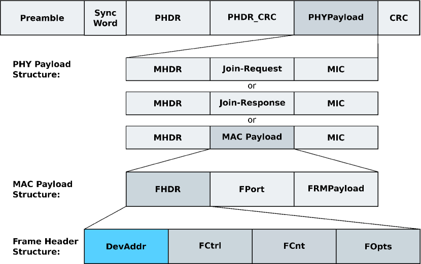
Figure 4: The LoRaWAN packet structure [34].

LoRa is a proprietary physical layer wireless protocol powering network layer protocols, such as LoRaWAN [34] long-range wide-area networks (LP-WAN) and Sidewalk [35]. LoRa defines all supported modulations and physical layer signaling. On the other hand, LoRaWAN defines a subset of all possible modulations and signal parameters, such as frequency allocations and channel widths. The physical layer of the LoRa protocol was patented by Semtech, and the specification of LoRaWAN is governed by the LoRa Alliance [34]. Work by security researchers have yielded SDR implementations of the physical LoRa layer [28, 5].

LoRaWAN uplink channels consists of 64 125 KHz wide channels (centered around $f_{c}=903.2+0.2k$ MHz where $k=0...63$) and 8 500 KHz wide channels (centered around $f_{c}=903+1.6(k-64)$ MHz where $k=64...71$). LoRaWAN downlink channels consists of 8 500 KHz wide channels (centered around $f_{c}=923.3+0.6k$ MHz where $k=0...7$) [36].

Address Information. We use the third byte after the sync word to enumerate the LoRa devices under test. Indeed, from the traffic we collected, the value of the third byte consistently changed between four values, corresponding to the IDs of the four YoLink devices under test. Incidentally, this third byte of the payload is part of the 32-bit device address (DevAddr) as specified in LoRaWAN frame format [34]. Furthermore, the first byte of DevAddr is used as a network identifier (NwkID), which is fixed for all devices in the same network. In this context, a network consists of a LoRa gateway and end-devices connected to that gateway.

Implementation. In our implementation, we scan LoRa devices listed in Table I using Algorithm 7. YoLink’s website does not specify whether or not their devices are LoRaWAN compatible. However we found that the sync words used by YoLink devices are different from the public sync word (0x3444) - needed for LoRaWAN compliance [34].

We observed that our YoLink devices only used two channels: 910.29 MHz for the end-devices (uplink) and 923.29 MHz for the gateway (downlink). Note that the uplink frequency is located between two official LoRaWAN frequencies. The YoLink’s downlink frequency (923.29 MHz) is very close to the LoRaWAN’s downlink channel zero (923.3 MHz). YoLink’s downlink bandwidth is 125 KHz and not 500 KHz, as defined by LoRaWAN. YoLink’s uplink bandwidth of 125 KHz agrees with LoRaWAN specification. Given that YoLink does not exactly follow LoRaWAN’s frequency allocations and channel widths, this gives further proof that YoLink devices are not LoRaWAN compatible.

The major challenge in receiving any Yolink traffic initially was in determining the network’s custom sync word, because the default SDR LoRa receiver [5] accepts only sync words with a value of zero. Sync word values containing 0x00 are forbidden in deployed networks and can only be used for testing. We overcame this challenge by modifying the LoRa receiver of [5]. Our implementation allows one to promiscuously listen for all sync words, as well as configure the bandwidth, the center frequency, the bitrate, and other parameters. A key advantage of scanning LoRa using an SDR implementation is that all sync words can be monitored simultaneously, whereas certified LoRa transceiver chips are programmed to receive a specific sync word.

V-D Z-Wave

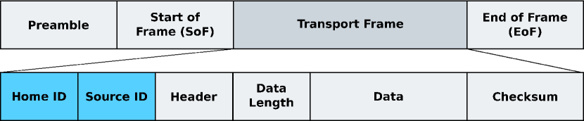
Figure 5: Z-Wave physical (PHY) and medium access control (MAC) layer frame structure [4].

Z-Wave is another proprietary physical layer wireless protocol, based on the ITU-T G.9959 specification [4]. It is used in smart home applications, most notably Ring Home Security Systems.

In the US, Z-Wave operates on the 900 MHz ISM band and comes in a few physical layer (PHY) variants, most importantly differentiated by its center frequency and bit rates (channel widths): 908.4 MHz at 9.6 Kbps (R1) and 40 Kbps (R2); 916 MHz at 100 Kbps (R3). Z-Wave long range PHYs at 912MHz and 921 MHz [9] are less common. For Z-Wave devices listed in Table I, IoT-Scan discovered traffic on the R2 and R3 PHYs, with corresponding channel widths of 40 KHz and 100 KHz respectively.

Address Information. Z-Wave packets contain two address-related data fields: the home (network) identifier, and the node (device) identifier. We use the single byte Source ID [37] to enumerate Z-Wave devices. Z-Wave supports up to 232 devices per network, hence this byte is sufficient to distinguish between devices on the same network. The Z-Wave primary controller (Z-Wave gateway) has a Source ID of 1. A Z-Wave device which has not been connected to a controller must use a Source ID of 0 before obtaining an actual non-zero Source ID. The Z-Wave network identifier or Home ID consists of 4 bytes that precede the node ID, as shown in Fig. 5. In the case of multiple overlapping networks, the Home ID can be used to distinguish between devices on different networks.

Implementation. R1 and R2 Z-Wave PHY implementations are available from Picod et al. [38] and scapy-radio [14]. We built the R3 Z-Wave PHY flowgraph based on the existing R2 PHY implementation, the only difference is that the bitrate/sampling rate has to be 2.5 times larger. IoT-Scan discovers Z-Wave devices by listening on the 908.4 MHz and 916 MHz channels. We then enumerate the Z-Wave packet’s source IDs with a custom made Z-Wave Wireshark dissector [39].

VI Experimental Evaluation

In this section, we perform an experimental evaluation of the scanning algorithms of IoT-Scan. We detail SDR implementation aspects, the experimental set-up (including the list of tested devices), and the experimental results.

VI-A Algorithm Implementation

The algorithms described in Section III do not go into details of SDR-level implementation. This section provides additional detail on the implementation of these algorithms. The main software components consist of GNU Radio 3.8 [13] and Scapy-radio 2.4.5 [40]. Scapy-radio is a pentest tool with RF capabilities, a modification of the Scapy toolkit [40]. Note that Scapy-radio currently supports GNU Radio version 3.7, and therefore we had to port several blocks to version 3.8. A significant feature improvement in GNU Radio 3.8 is the default automatic gain control (AGC) supported by the USRP Source block, which improves receiver reliability.

1)   Flowgraph control

We implement the scanning algorithms described in Section III in Python. Signal processing parameters, such as the SDR center frequency, the channel frequency offsets, and the channel bandwidths, are managed by a GNU Radio flowgraph. The GNU Radio flowgraph is imported from the main application as a Python module and is controlled with its native Python API. This allows for dynamic control of flowgraph parameters during the runtime of the flowgraph. Controlling the flowgraph in this way is crucial for correct time-keeping of the experiments, as it allows to compensate for flowgraph startup delays of several seconds resulting from the initialization of the USRP hardware driver library UHD [41], which sets up the SDR hardware before the flowgraph can be executed.

2)   Signal processing

The process of converting an unfiltered full-bandwidth signal from an SDR source into the receive chain (i.e, the sequence of DSP blocks connected serially starting with radio source, demodulator, filter, and clock recovery) of a particular protocol is referred to as channelization [42]. Channelization comprises three signal processing steps: frequency translation (from the center frequency of the raw radio signal to the center frequency of the desired channel), channel filtering (filtering out other protocols and potential interference), and re-sampling (down conversion) to reduce the computational load.

Channelization is particularly important in multiprotocol scanning, since it reduces the computational complexity of the receivers by reducing the sampling rate. Multiprotocol scans require parallel decoding of two or more receive chains which can overwhelm the capabilities of a typical host computer if the processing chain in the flowgraph is not correctly optimized.

Reducing the sample rate relies on Nyquist theorem, which dictates that the sample rate of a signal be at least twice the signal’s bandwidth, in order to not lose any information (in other words, to not have signal aliasing or ambiguity in reconstructing the original signal that was transmitted). Channel filtering reduces the total captured signal bandwidth down to the bandwidth of a single protocol channel in a given received chain. The reduced sample rate matches the reduced bandwidth of the filtered signal, such that the Nyquist rate condition still holds after channelization.

VI-B Experimental Setup

Table I: Tested IoT devices.

.

We implemented all the scanning algorithms described in Section III on a single SDR device, namely a USRP B200 device [18], with a PC capable enough to handle data processing in real-time without dropping samples (i.e., overflowing buffers). Thus, all our experiments were run on a ThinkCentre 8 Core Intel i7 running Ubuntu 20.04.

The devices used in the experiments are listed in Table I. Traffic of the BLE and Zigbee devices were statistically analyzed to derive the parameters of the theoretical traffic model introduced in Section IV-B. Note that we did not analyze transmission statistics of low-power Z-Wave and LoRa devices due to their periodic transmission patterns (devices transmit once every hour or so).

‘

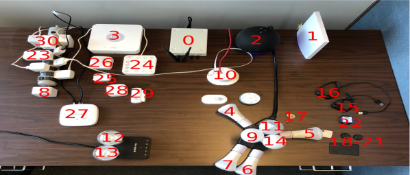
Figure 6: The experimental setup for the tested IoT devices, see Table I for the numbering. The SDR is labeled with number 0.

All scanning experiments were based on IoT devices under our control. Any foreign device from the environment was filtered out. In order to only account for our devices, we initially enumerated them with a passive scan inside an RF shielded box (Ramsey box STE3500) to determine their addresses.

We conducted all scanning experiments using the default network configuration of the respective devices and protocols, i.e., by setting them up via their respective gateways and/or apps (wherever applicable) in preparation of any experiments. During all the experiments, the tested devices (see Table I) were in an idle state, i.e., not actively used by an operator. Manually operating devices in a way that generates network communication, e.g., actuating Zigbee lights via the Amazon Alexa smartphone app, would impact scanning performance. We expect the results presented in this section to be conservative estimates of the scanning time, since generating additional traffic from the devices should speed up the discovery of the devices. All devices were located near the SDR, as shown in Fig. 6.

Regarding the parameters of the algorithms, the channel dwell time (i.e, the scanning time of each channel in each round) was set to 1 second. Exceptions are the channel dwell time during active scan of Zigbee (set to 0.2 s), and in Section 5 where we evaluate the impact of different channel dwell times on the performance of the algorithms. In each experiment, the total scan time was set to be long enough for all devices to be discovered.

When scanning each individual protocol, we set the instantaneous bandwidth parameter in accordance with the respective protocol’s bitrate. Specifically, BLE’s channel bandwidth was set to 1 MHz, Zigbee to 2 MHz, LoRa to 125 KHz, and Z-Wave to 40/100 KHz. When implementing multiprotocol scanning algorithms, we used wider bandwidth to fit the bandwidth of each protocol and channel spacing in between. Both the Zigbee/BLE and Z-Wave/LoRa and multi-protocols experiment used 8 MHz of bandwidth, which in each case was sufficient to simultaneously capture channels from each protocol, as discussed in the sequel.

VI-C Results

In this section, we discuss experimental results of the scanning algorithms. The figures show the sample means and 95% confidence intervals of the order statistics of the discovery time of the $n$-th device (see Eqs. (4) and (5)). Each point represents an average over 10 experiments with identical parameters.

1)   Passive Zigbee and BLE Scans and Comparison with Theoretical Model

We first evaluate the performance of the passive scanning algorithms (Algorithm 2) for Zigbee and BLE devices, and compare those with the expected discovery times based on the theoretical model described in Section IV-B.

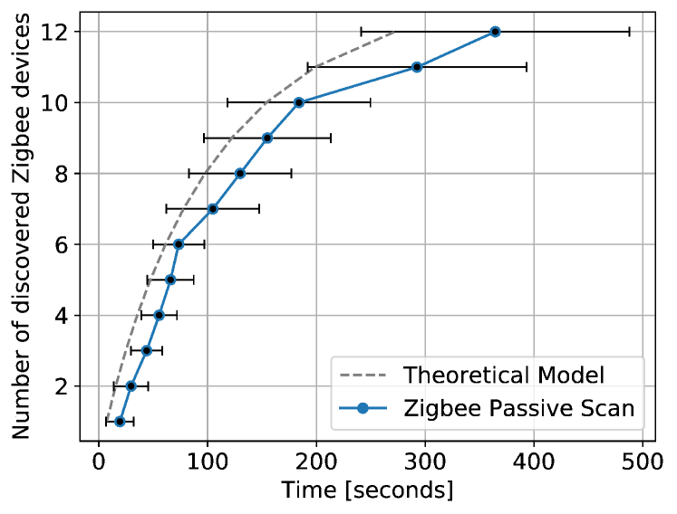
Figure 7: Zigbee theoretical model and experimental passive scan results. The 95% confidence interval indicates a good fit.

To build the theoretical traffic model (see Section IV-B), we measured device characteristics of our tested devices by running one long continuous scan of 100 minutes on every Zigbee channel and on every BLE advertising channel, in order to collect a baseline of traffic for each device. The traffic statistics are shown in Table I. We set $\Delta t=0.1$s, in Eq. (15) to compute $p_{i}$ for each device (this ensures that $\Pr(Z\geq 2)$ is negligible). We then use Eq. (10) to compute the expectation of the order statistics of the discovery time of devices. Note that for Zigbee, we replace $p_{i}$ by $p_{i}/16$, since with Algorithm 2, the SDR listens to only one out of the 16 Zigbee channels at a time.

Fig. 7 shows curves for the experimental results of Zigbee passive scanning and the theoretical model. The model fits inside most of the 95% confidence intervals. This shows that our passive scan implementation is close to the best performance possible, and our testbed has minimal packet losses. The deviation from the model could be attributed to interference (e.g., from Wi-Fi) and the fact that transmissions of some Zigbee devices are not memoryless.

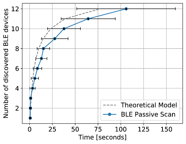
Figure 8: BLE passive scan results align closely with the theoretical model.

Fig. 8 shows experimental results for BLE passive scanning and the theoretical benchmark. The measured discovery times again fit the model well. Since all BLE advertising channels are equivalent, scanning is performed on channel 37 only. Note that BLE device discovery can only be performed as a passive scan, since BLE does not allow for broadcast-type scan requests as performed in Zigbee. While BLE scan requests could be a useful active scanning technique for gathering additional device data, they are always directed scans, i.e., they require knowledge of the target device’s address.

2)   Active Zigbee Scan

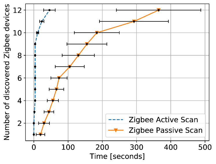
Figure 9: Zigbee active versus passive scan.

We next evaluate the performance of active scanning (Algorithm 4) and compare it to passive scanning in the context of Zigbee. Fig. 9 shows that the passive discovery of 12 Zigbee devices takes 365 seconds on average while active Zigbee discovery takes only 46 seconds, i.e., a reduction of 87% in the scan time. While active scanning discovers the 12 devices within one minute, passive scanning discovers only 4 devices within one minute.

Note that Zigbee supports up to 64,000 nodes per network. It is conceivable that the improvement of active scan over passive scan would be even more significant with a larger number of nodes. Zigbee routers and coordinators are typically continuously active and will reply to beacon requests, which contributes to the discovery of several devices almost immediately during the active scan, whereas end-devices are usually optimized for power saving, and may not respond to beacon requests. However, since end devices are on the same channel as their coordinator, limiting the second phase of the active scan to the known active channels significantly speeds up discovery by virtue of spending more time on each relevant channel. Among our tested devices, we have three Zigbee coordinators occupying three channels: GE Link/Quirky hub on channel 11, IKEA Gateway on channel 15, and Amazon echo 4.0 on channel 20. As a result, the second phase of the active scan (cf. Algorithm 4, line 4) cycles through 3 instead of 16 channels, shortening the detection speed by a factor of roughly $16/3=5.333$ for the remaining end-devices.

3)   Zigbee and BLE Multiprotocol Scan

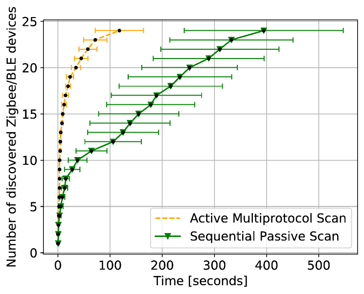
Figure 10: Zigbee/BLE multiprotocol active scan vs. sequential passive scan.

We next evaluate the performance of active multiprotocol Zigbee and BLE scan (Algorithm 8) and compare it to sequential passive scan (Algorithm 2). Sequential passive scan consists of passive BLE scan followed by passive Zigbee scan. Sequential passive scan enumerates the 24 considered devices in 395 seconds on average, while active multiprotocol Zigbee and BLE scan takes 118 seconds on average, which corresponds to a 70% improvement (Fig. 10). Within 1 minute active multiprotocol scan discovers 22 devices while sequential scan discovers only 10. Breaking down sequential passive scan into two: the first 106 seconds corresponds to a BLE passive scan, followed by 289 seconds of Zigbee scan, which is consistent with the results shown in Figs. 7 and 8.

The speed-up is achieved because of two aspects: active scan and multiprotocol scan. Zigbee active scan narrows the search down from 16 to only 3 channels. Multiprotocol scan supports reception of one Zigbee and one BLE channel in parallel. Note that parallel reception is possible only if the two channels fit within the instantaneous bandwidth. As mentioned earlier, the instantaneous bandwidth for multiprotocol scan was set to 8 MHz. Three Zigbee active channels were identified, namely channel 11, 15, and 20. BLE has three well-known advertising channels, namely 37, 38, and 39. BLE channel 37 and Zigbee channel 11 can be received in parallel as well as BLE channel 38 and Zigbee channel 15. However, Zigbee channel 20 and BLE channel 39 are scanned separately since they do not fit within the same instantaneous bandwidth.

4)   Z-Wave and LoRa Multiptotocol Scan

We next evaluate the performance of passive multiprotocol LoRa and Z-Wave scan on 900 MHz band (Algorithm 7) and compare it to sequential passive scan (Algorithm 2). Passive multiprotocol scan consists of scanning each of 3 frequency channels (2 Z-Wave and 1 LoRa) in a round robin fashion. The passive scanning operation visits the LoRa and Z-Wave channel in a round-robin fashion, one at a time. Due to having 2 Z-Wave channels (908.4 and 916 MHz) and only 1 LoRa channel (910.29 MHz), Z-Wave has an advantage in passive scanning.

Fig. 11 shows that sequential LoRa and Z-Wave scan takes about 8.1 hours on average while multiprotocol Z-Wave and LoRa scan takes 2.5 hours, which represents a reduction of about 70% in the discovery time. Within a single hour passive scan discovers less than 1 device on average while multiprotocol scan discovers 5 out of the 7 devices. This significant speed-up is achieved because multiprotocol scan receives all three channels (from the two protocols) in parallel, namely 908.4 MHz (Z-Wave R2 PHY), 910.23 MHz (LoRa uplink), and 916 MHz (Z-Wave R3 PHY).

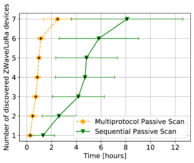
Figure 11: Multiprotocol passive scan (Z-Wave, LoRa)

5)   Channel Dwell Time

We last examine the impact of properly setting the value of the channel dwell parameter, which is an input to several of the algorithms. Each trial measures the time to passively scan 12 BLE and 12 Zigbee devices. Passive Zigbee scan hops between 3 active Zigbee channels. A passive BLE scan involves channel hopping between three advertising BLE channels. Our experiments indicate that the scanning times do not differ significantly for channel dwell times of 0.1, 1, and 3 seconds. Fig. 12 shows the channel dwell time experiment for Zigbee, but similar results hold for BLE. Thus, in all our experiments, we chose a value of 1 second for the channel dwell times, the only exception being in the first phase of Zigbee active scan, where the dwell time was set to 0.2 seconds (which was sufficient to receive beacon responses and move on).

Figure 12: Zigbee passive scan discovery times for channel dwell times of 0.1, 1, and 3 seconds.

VII Conclusion

We presented IoT-Scan, a protocol-agnostic and extensible network reconnaissance tool for the Internet of Things that can be employed for network monitoring and security auditing. IoT-Scan leverages the capabilities of SDRs to process multiple streams in parallel. Accordingly, we introduced several scanning algorithms and evaluated them both theoretically and experimentally. Using the theoretical model, we showed that our implementation is efficient and achieves minimal packet loss in reception. We implemented multi-protocol, multi-channel scanning both on the 2.4GHz band for Zigbee and BLE, and on the 900 MHz band for LoRa and Z-Wave, and demonstrated significant improvement over sequential passive scanning.

Our SDR implementations should prove especially useful in overcoming the incompatibility of different protocols based on the same PHY layer. For instance, besides Zigbee, there exist several IoT protocols based on the IEEE 802.15.4 standard, such as Thread [43] and WirelessHART [44]. We expect that these protocols could readily be integrated into IoT-Scan.

Our SDR implementations of LoRa overcomes a significant limitation of existing network cards for this protocol. Specifically, the LoRa protocol encodes the network ID using the synchronization word (sync word) at the PHY layer. Common network cards are programmed to only receive packets containing a specific sync word and therefore cannot detect devices belonging to other LoRa networks. In contrast, our SDR implementation of a LoRa receiver gives us the opportunity to listen promiscuously to LoRa traffic. This flexibility is achieved by skipping the network address filtering enforced by the sync word, and allows us to receive all LoRa traffic regardless of the network ID. Likewise, common Z-Wave devices do not support promiscuous mode, supposedly to avoid intercepting traffic from other networks [45]. Our SDR implementation overrides this security-by-obscurity feature of Z-Wave.

The design of IoT-Scan does not raise ethical issues by itself. However, like other penetration testing tools, usage of this tool does require explicit consent from the owners of the devices under test. Specifically, active scanning, while brief, may interfere with existing network traffic and delay time-sensitive communication. A major advantage of IoT-Scan versus a tool like Nmap is that it also supports a passive scanning mode, which does not generate traffic. Nevertheless, passive scanning also requires owner consent as this may otherwise expose private information or identifiable addresses. Public releases of data logs of IoT traffic captured with IoT-Scan must therefore be properly anonymized.

This paper opens several avenues for future work. First, one could explore FPGA implementations of IoT-Scan to increase the number of channels and protocols that can be decoded in parallel and further speed up the discovery of IoT devices. While this should yield useful performance improvements, we expect that such implementations would still rely on the algorithms introduced in Section III. Another interesting research avenue lies in the design of active scanning methods for LoRa and Z-Wave, as devices in these protocols transmit sparingly.

We plan to make our implementation of IoT-Scan broadly available to the research community to facilitate such innovations, and more generally strengthen the visibility and security of IoT devices. Anonymized time-series data extracted from PCAP files containing recorded device traffic are available at https://github.com/nislab/iot-scan/.

References

- [1] Ericsson. (2020) Internet of Things Forecast. [Online]. Available: https://www.ericsson.com/en/mobility-report/internet-of-things-forecast
- [2] Bluetooth Special Interest Group (SIG). (2016) Bluetooth Core Specification. v5.0. [Online]. Available: https://www.bluetooth.com/specifications/specs/core-specification/
- [3] IEEE Standards Association, “Ieee standard for low-rate wireless networks,” IEEE Std 802.15.4-2015 (Revision of IEEE Std 802.15.4-2011), pp. 1–709, 2016.
- [4] International Telecommunication Union. (2015) G.9959: Short range narrow-band digital radiocommunication transceivers - PHY, MAC, SAR and LLC layer specifications. [Online]. Available: https://www.itu.int/rec/T-REC-G.9959
- [5] J. Tapparel, O. Afisiadis, P. Mayoraz, A. Balatsoukas-Stimming, and A. Burg, “An open-source lora physical layer prototype on gnu radio,” in 2020 IEEE 21st International Workshop on Signal Processing Advances in Wireless Communications (SPAWC), 2020, pp. 1–5.
- [6] J. Ortiz, C. Crawford, and F. Le, “DeviceMien: network device behavior modeling for identifying unknown IoT devices,” in Proceedings of the International Conference on Internet of Things Design and Implementation. New York, NY, USA: ACM, Apr 2019, pp. 106–117. [Online]. Available: https://dl.acm.org/doi/10.1145/3302505.3310073
- [7] D. Y. Huang, N. Apthorpe, F. Li, G. Acar, and N. Feamster, “IoT Inspector,” Proceedings of the ACM on Interactive, Mobile, Wearable and Ubiquitous Technologies, vol. 4, no. 2, pp. 1–21, Jun 2020. [Online]. Available: https://dl.acm.org/doi/10.1145/3397333
- [8] US Congress, “H.R.1668 - IoT Cybersecurity Improvement Act of 2020,” 2020. [Online]. Available: https://www.congress.gov/bill/116th-congress/house-bill/1668
- [9] M. Klein. (2020) What is Z-Wave Long Range and How Does it Differ from Z-Wave? [Online]. Available: https://z-wavealliance.org/what-is-z-wave-long-range-and-how-does-it-differ-from-z-wave/
- [10] G. F. Lyon, Nmap network scanning: The official Nmap project guide to network discovery and security scanning, 2nd ed. Sunnyvale, CA, USA: Insecure.Com LLC, 2008.
- [11] CSA. (2021, Dec) Matter: Smart home device solution. [Online]. Available: https://csa-iot.org/all-solutions/matter/
- [12] T. Ulversoy, “Software defined radio: Challenges and opportunities,” IEEE Communications Surveys & Tutorials, vol. 12, no. 4, pp. 531–550, 2010.
- [13] GNU Radio Project. (2022) GNU Radio. [Online]. Available: https://www.gnuradio.org
- [14] Bastille Research. (2015) scapy-radio. [Online]. Available: https://github.com/BastilleResearch/scapy-radio
- [15] Y. He, J. Fang, J. Zhang, H. Shen, K. Tan, and Y. Zhang, “MPAP: Virtualization architecture for heterogenous wireless APs,” ACM SIGCOMM Computer Communication Review, vol. 40, no. 4, pp. 475–476, Aug 2010. [Online]. Available: https://dl.acm.org/doi/10.1145/1851275.1851271
- [16] P. Flajolet, D. Gardy, and L. Thimonier, “Birthday paradox, coupon collectors, caching algorithms and self-organizing search,” Discrete Applied Mathematics, vol. 39, no. 3, pp. 207–229, Nov 1992.
- [17] E. Anceaume, Y. Busnel, and B. Sericola, “New results on a generalized coupon collector problem using markov chains,” Journal of Applied Probability, vol. 52, no. 2, p. 405–418, 2015.
- [18] Ettus Research. (2022) Usrp b200. [Online]. Available: https://www.ettus.com/all-products/ub200-kit/
- [19] A. Heinrich, M. Stute, and M. Hollick, “BTLEmap: Nmap for Bluetooth Low Energy,” in Proceedings of the 13th ACM Conference on Security and Privacy in Wireless and Mobile Networks, ser. WiSec ’20. Association for Computing Machinery, 2020, p. 331–333. [Online]. Available: https://doi.org/10.1145/3395351.3401796
- [20] J. Tournier, F. Lesueur, F. Le Mouël, L. Guyon, and H. Ben-Hassine, “IoTMap: A protocol-agnostic multi-layer system to detect application patterns in IoT networks,” in 10th International Conference on the Internet of Things (IoT 2020), Malmö, Sweden, Oct. 2020.
- [21] J. Mikulskis, J. K. Becker, S. Gvozdenovic, and D. Starobinski, “Snout: An extensible iot pen-testing tool,” in Proceedings of the 2019 ACM SIGSAC Conference on Computer and Communications Security, ser. CCS ’19. New York, NY, USA: Association for Computing Machinery, 2019, p. 2529–2531. [Online]. Available: https://doi.org/10.1145/3319535.3363248
- [22] S. Bak and Y.-J. Suh, “Designing and implementing an enhanced bluetooth low energy scanner with user-level channel awareness and simultaneous channel scanning,” vol. 102, no. 3. The Institute of Electronics, Information and Communication Engineers, 2019, pp. 640–644.
- [23] C. D. Kilgour, “A Bluetooth low-energy capture and analysis tool using software-defined radio,” Master’s Thesis, Simon Fraser University, 2013. [Online]. Available: http://summit.sfu.ca/item/12931
- [24] Wi-Fi Alliance. (2022) What are passive and active scanning? [Online]. Available: https://www.wi-fi.org/knowledge-center/faq/what-are-passive-and-active-scanning
- [25] W. Park, D. Ryoo, C. Joo, and S. Bahk, “Bless: Ble-aided swift wi-fi scanning in multi-protocol iot networks,” in IEEE INFOCOM 2021-IEEE Conference on Computer Communications, 2021, pp. 1–10.
- [26] J. Hall, B. Ramsey, M. Rice, and T. Lacey, “Z-wave network reconnaissance and transceiver fingerprinting using software-defined radios,” in International Conference on Cyber Warfare and Security. Reading, United Kingdom: Academic Conferences International Limited, 2016, p. 163.
- [27] L. Choong, “Multi-channel ieee 802.15.4 packet capture using software defined radio,” UCLA Networked & Embedded Sensing Lab, vol. 3, pp. 1–20, 2009.
- [28] P. Robyns, P. Quax, W. Lamotte, and W. Thenaers, “A multi-channel software decoder for the lora modulation scheme,” in Proceedings of the 3rd International Conference on Internet of Things, Big Data and Security (IoTBDS 2018), 2018, pp. 41–51.
- [29] B. Schmeiser, “Batch size effects in the analysis of simulation output,” Operations Research, vol. 30, no. 3, pp. 556–568, 1982.
- [30] Connectivity Standards Alliance. (2021) Zigbee – The Full-Stack Solution for All Smart Devices. [Online]. Available: https://csa-iot.org/all-solutions/zigbee/
- [31] N. K. Gupta, Inside Bluetooth Low Energy, 2nd ed. Boston, London: Artech House, 2016.
- [32] J. K. Becker, D. Li, and D. Starobinski, “Tracking anonymized bluetooth devices,” vol. 2019, no. 3, Jul. 2019, pp. 50–65.
- [33] G. Celosia and M. Cunche, “Discontinued privacy: Personal data leaks in apple bluetooth-low-energy continuity protocols,” vol. 2020. De Gruyter Open, 2020, pp. 26–46.
- [34] LoRa Alliance. (2018, July) Lorawan® specification v1.0.3. [Online]. Available: https://lora-alliance.org/wp-content/uploads/2020/11/lorawan1.0.3.pdf
- [35] Jon Callas. (2022) Understanding amazon sidewalk. [Online]. Available: https://www.eff.org/deeplinks/2021/06/understanding-amazon-sidewalk
- [36] LoRa Alliance, “LoRaWAN® Regional Parameters,” 2021. [Online]. Available: https://lora-alliance.org/wp-content/uploads/2021/05/RP002-1.0.3-FINAL-1.pdf
- [37] C. W. Badenhop, S. R. Graham, B. W. Ramsey, B. E. Mullins, and L. O. Mailloux, “The z-wave routing protocol and its security implications,” Computers & Security, vol. 68, pp. 112–129, 2017.
- [38] J.-C. D. Jean-Michel Picod, Arnaud Lebrun, “Bringing Software Defined Radio to the Penetration Testing Community,” Black Hat, 2014. [Online]. Available: https://www.blackhat.com/docs/us-14/materials/us-14-Picod-Bringing-Software-Defined-Radio-To-The-Penetration-Testing-Community-WP.pdf
- [39] B. Lipton. (2016) wireshark. [Online]. Available: https://github.com/LiptonB/wireshark
- [40] SecDev. (2021) Scapy: the Python-based interactive packet manipulation program & library. [Online]. Available: https://github.com/secdev/scapy
- [41] Ettus Research. (2021) uhd. [Online]. Available: https://github.com/EttusResearch/uhd.git
- [42] Marija Dimitrijevic. (2018) Replacing many RF receivers with only ONE using Channelization. [Online]. Available: https://www.ettus.com/wp-content/uploads/2018/12/Channelization_-_Article_.pdf
- [43] Thread Group. (2022) What is Thread? [Online]. Available: https://www.threadgroup.org/What-is-Thread/Overview
- [44] FieldComm Group, “WirelessHART. HART WITHOUT THE WIRES,” 2021. [Online]. Available: https://www.fieldcommgroup.org/technologies/wirelesshart
- [45] D. Dragomir, L. Gheorghe, S. Costea, and A. Radovici, “A survey on secure communication protocols for iot systems,” in 2016 International Workshop on Secure Internet of Things (SIoT), 2016, pp. 47–62.