Adversarial Robustness through the Lens of Convolutional Filters

Abstract

Deep learning models are intrinsically sensitive to distribution shifts in the input data. In particular, small, barely perceivable perturbations to the input data can force models to make wrong predictions with high confidence. An common defense mechanism is regularization through adversarial training which injects worst-case perturbations back into training to strengthen the decision boundaries, and to reduce overfitting. In this context, we perform an investigation of $3\times 3$ convolution filters that form in adversarially-trained models. Filters are extracted from 71 public models of the $\ell_{\infty}$-RobustBench CIFAR-10/100 and ImageNet1k leaderboard and compared to filters extracted from models built on the same architectures but trained without robust regularization. We observe that adversarially-robust models appear to form more diverse, less sparse, and more orthogonal convolution filters than their normal counterparts. The largest differences between robust and normal models are found in the deepest layers, and the very first convolution layer, which consistently and predominantly forms filters that can partially eliminate perturbations, irrespective of the architecture.

Data & Project website:
https://github.com/paulgavrikov/cvpr22w_RobustnessThroughTheLens

1 Introduction

Convolutional Neural Networks (CNNs) have been successfully applied to solve many different computer vision problems. As the state of the art has been consequently pushed, research was mostly devoted at improving the performance (validation accuracy, along speed and others). However, recently it has been shown that these models are sensitive to distribution shifts in image data. Even small, for humans almost imperceptible, perturbations applied to input images can force the networks to make high-confidence, false predictions on samples that would otherwise have been classified correctly[1, 2]. Normal training on off-the-shelf architectures typically results in zero validation accuracy against perturbed samples. This raises the question on whether current deep learning models should be used in safety-critical applications [3, 4, 5]. Consequently, researchers have devoted their work on studying the sensitivity to distribution shifts e.g. by finding and understanding adversarial inputs [6, 7], and building defenses to those [8, 9, 10, 11]. While most explanatory methods study the distribution shifts in the input data and activations, we propose to evaluate differences in learned convolutional filters and, therefore, round out previous findings through a different perspective. More specifically, we investigate shifts in the dominantly used $3\times 3$ filters in CNN classification models trained on CIFAR-10/100[12] and ImageNet1k[13] datasets that were trained to withstand $\ell_{\infty}$-bound adversarial attacks. However, we believe that our results also apply to other tasks, datasets, and perhaps even to other attack vectors. We summarize our key contributions and findings as follows:

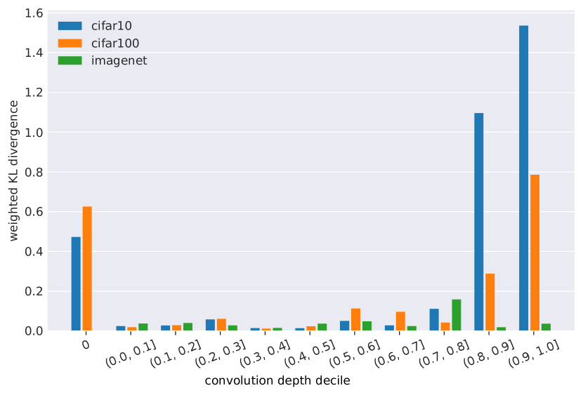
Figure 1: Filter structure divergence between learned $3\times 3$ filter structures of robust and normal models by depth decile. The first convolutional layer is displayed separately. The most significant shifts (large KL values) appear in the primary convolution layer and deeper stages.

• We collect 71 public robust models with 13 different architectures trained on 3 image datasets. These models contain a total of 615,863,744 filters with a size of $3\times 3$. Additionally, the therein used architectures are trained from scratch without the employed robustness regularizations.

• We show an in depth empirical comparison of learned $3\times\leavevmode\nobreak\ 3$ convolution filters between robust and normal models. The resulting filter dataset is made available publicly[14].

• Our analysis shows that differences in filter structure increase with layer depth, but significantly explode towards the end of the model, with a dominant outlier showing in the primary convolution layer.

• We visualize the primary layer of robust models and its activations, and observe a large presence of thresholding-filters that can remove perturbations from regions of interest.

• We discover that robust models appear to form more diverse, less sparse, and more orthogonal convolution filters.

2 Related Work

Adversarial attacks and defenses

Let $\mathcal{F}$ denote a model parameterized by $\theta$, $x$ an input sample with the corresponding class label $y$, and $\mathcal{L}$ the loss function. Adversarial attacks attempt to maximize the loss $\mathcal{L}$ by finding an additive perturbation to an input sample $x^{\prime}$ in the $\mathcal{B}_{\epsilon}(x)$ ball that is centered at $x$ with a radius of $\epsilon$. $\|\cdot\|_{p}$ depicts the $\ell_{p}$-norm with usually $p=2$ or $\infty$.

$$\begin{gathered}\displaystyle\max_{x^{\prime}\in\mathcal{B}_{\epsilon}(x)}\mathcal{L}\left(\mathcal{F}\left(x^{\prime};\theta\right),y\right)\\ \mathcal{B}_{\epsilon}(x)=\{x^{\prime}:\|x-x^{\prime}\|_{p}\leq\epsilon\}\end{gathered}$$ (1)

On the other hand, to achieve robustness, the loss caused by the perturbation has to be mitigated by finding more suitable set of model parameters $\theta$. One of the most successful approaches is seen in adversarial training[10] where adversarial perturbations are found and reintroduced into training, alongside with the inclusion of external data [15].

Robustness evaluation

A common framework for adversarial robustness benchmarks is RobustBench [16]. The framework applies $\text{APGD}_{ce}$, $\text{APGD}_{t}$ [10, 17], FAB [18], and Square [19] attacks via AutoAttack [17] to obtain a comparable robustness accuracy. Perturbations are obtained from $\mathcal{B}_{\epsilon}$ with $p=2,\epsilon=0.5$ on CIFAR-10, as well as $p=\infty,\epsilon=8/255$ on CIFAR-10/100, and $p=\infty,\epsilon=4/255$ on ImageNet1k, respectively. This methodology was questioned more recently, as the established $\epsilon$-thresholds are disputed as being too large and generate perturbations that can easily be detected[20].

Filter analysis

Yosinski et. al. [21] studied filters of ImageNet1k CNN classification models and concluded that early vision layers will form similar features, namely Gabor-filters and color-blobs, independent of task or dataset. On the other hand, deeper layers will capture specifics of the dataset by forming increasingly specialized filters. A thorough analysis of filters limited to a specific InceptionV1 [22] model trained on ImageNet1k was presented in [23, 24, 25, 26, 27, 28, 29, 30, 31]. The authors back Yosinski et. al. and even go beyond by arguing that models are not only forming similar filters, but also connections (i.e. consecutive transformations). As model capacity increased, little to no research was devoted to understanding learned filters. More recently, we presented an empirical analysis of 1.4B filters obtained from models with different architectures, datasets, and training tasks [32]. We also introduced a PCA-based method to compare the structure of learned filters, alongside two metrics to evaluate their quality (sparsity and variance entropy). Our findings showed that learned filter distributions remain largely similar across various splits, but many models show a large ration of degradation in filters. Within our study, we also briefly touched up on filter quality in robust models on ImageNet1k and noticed that robust models form more diverse filters than their non-robust counterparts. The presented study builds on top of this previous work, and explores differences specifically focused at the robustness aspect and with significantly more details. Instead of comparing robust models to a large collection of various ImageNet1k-classifiers, we compare differences to the same architectures trained without robustness regularization to allow for a less biased analysis. Additionally, we extend our analysis to other datasets, refine previous quality metrics, and evaluate a new metric to capture the orthogonality of filterbanks. Regarding robust filter analysis, we observe that models trained for $\ell_{\infty}$ robustness form thresholding filters in early vision which are able to remove perturbations.

Connection to other model analysis

[33] presented the Lottery Ticket Hypothesis, which claims that CNNs form various redundant subnetworks that each increase the odds of finding a solution. Once a solution was found, the “loosing” subnetworks can be removed without any significant impacts on accuracy. Upon that, [34] observed that adversarial samples activate channels of the feature extractor more uniformly, and with larger magnitudes, and propose to suppress channels to increase robustness. Instead of suppressing channels, [35] showed that enhancing subnetworks can boost robustness to adversarial perturbations. [36] argue that adversarially-trained networks transfer better as they form richer representations. We hypothesize that these findings correlate with filter quality and believe that degenerated filters are the “loosing” subnetworks, that are activated by adversarial attacks. Improving the filter quality, in theory, should be a necessary, but not sufficient criterion to achieve robustness.

3 Methods

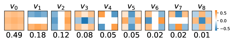
(a) All filters.

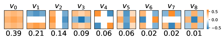
(b) Filters from robust models.

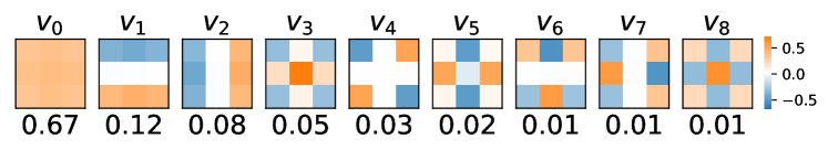
(c) Filters from normal models.

Figure 2: Filter basis and (cumulative) explained variance ratio per component (below) for filters from 2(a) all models, 2(b) adversarially-robust models, 2(c) normal models. Basis vectors are sorted by decreasing variance.

For the following sections, let $\boldsymbol{W}^{(i)}\in\mathbb{R}^{c_{\text{out}}\times c_{\text{in}}\times k_{1}\times k_{2}}$ be the layer weight of the $i$-th convolution layer with $c_{\text{in}}$ input-channels, $c_{\text{out}}$ output-channels, and $\boldsymbol{F}\in\boldsymbol{W}^{(i)}$ being a filter with shape $k_{1}\times k_{2}$ (here: $k_{1}=k_{2}=3$). For the following methods we reshape the layer weights into matrices that represent stacks of $n=c_{\text{out}}\times c_{\text{in}}$ flattened convolution filters:

$$\boldsymbol{W}^{(i)}\in\mathbb{R}^{c_{\text{out}}\times c_{\text{in}}\times k_{1}\times k_{2}}\rightarrow\boldsymbol{W}^{(i)}\in\mathbb{R}^{n\times(k_{1}\cdot k_{2})}$$ (2)

Comparing filter structure

As in [32] we perform a principal component analysis (PCA) via singular-value decomposition (SVD)[37] to understand the filter structure. In this work, however, we aim at reducing the previously hefty impact of sparse filters, by removing them from layer weights (for details see the next paragraph). Then we normalize each filter $\boldsymbol{F}\in\boldsymbol{W}^{(i)}$ individually to $\boldsymbol{F}^{\prime}$:

$$\begin{split}\displaystyle d_{i}&=\max_{i,j}\left|\boldsymbol{F}_{ij}\right|\\ \boldsymbol{F}_{ij}^{\prime}&=\left.\begin{cases}\boldsymbol{F}_{ij}/d_{i},&\text{if }d_{i}\neq 0\\ \boldsymbol{F}_{ij},&\text{else}\end{cases}\right.\\ \end{split}$$ (3)

The resulting layer weight matrix is centered and decomposed via SVD into a ${n\times k_{1}\cdot k_{2}}$ rotation matrix $\boldsymbol{U}$, a $k_{1}\cdot k_{2}\times k_{1}\cdot k_{2}$ diagonal scaling matrix $\boldsymbol{\Sigma}$, and a $k_{1}\cdot k_{2}\times k_{1}\cdot k_{2}$ rotation matrix $\boldsymbol{V}^{T}$. The diagonal entries $\sigma_{i},i=0,\dotsc,n-1$ of $\boldsymbol{\Sigma}$ form the singular values in decreasing order of their explained variance. The row vectors $v_{i},i=0,\dotsc,k_{1}\cdot k_{2}-1$ in $\boldsymbol{V}^{T}$ are called principal components/basis vectors. Every row vector $c_{ij},j=0,\dotsc,k_{1}\cdot k_{2}-1$ in $\boldsymbol{U}$ is the coefficient vector for $F^{\prime}_{i}$.

$$\begin{split}\boldsymbol{W}-\bar{\boldsymbol{W}}&=\boldsymbol{U}\boldsymbol{\Sigma}\boldsymbol{V}^{T}\\ \end{split}$$ (4)

Where $\bar{\boldsymbol{W}}$ denotes the vector of column-wise mean values of any matrix $\boldsymbol{W}$. We can then measure the explained variance ratio $\hat{a}$ of each principal component.

$$\begin{split}{a}&={(\boldsymbol{\Sigma}\boldsymbol{I})^{2}}/{(n-1)}\\ \hat{a}&={{a}}/{\|{a}\|_{1}}\end{split}$$ (5)

The sum of principal components $v_{i}$ weighted by the coefficients $c_{i}$ allows to reconstruct every scaled filter $\boldsymbol{F^{\prime}}\in\boldsymbol{W}^{(i)}$.

$$\begin{split}\displaystyle\boldsymbol{F}^{\prime}&=\sum_{i}c_{i}v_{i}+\bar{\boldsymbol{W}}_{i}\end{split}$$ (6)

Measuring layer quality

A static measurement of the layer quality (meaning by only using learned parameters) can be obtained by measuring the ratio of filters where all weights are near-zero (sparsity) as these filters do not contribute to the feature maps due to their low magnitudes. We apply the criterion presented in [32] and call a filter $\boldsymbol{F}\in\boldsymbol{W}^{(i)}$ sparse if $\max|\boldsymbol{F}|\leq\max|\boldsymbol{W}^{(i)}|/100$. The ratio is then defined by:

$$\begin{split}|\{\boldsymbol{F}|\boldsymbol{F}\in\boldsymbol{W}^{(i)}\land(\forall x\in\boldsymbol{F}:-\epsilon_{0}\leq x\leq\epsilon_{0})\}|/n\end{split}$$ (7)

Additionally, it is possible to quantify the diversity of filter structure in a given layer. We fit the PCA to individual layer weights $\boldsymbol{W}^{(i)}$ without normalization of filters and again remove sparse filters. The diversity can be then estimated by the non-negative $log_{10}$ entropy of the explained variance of each basis vector $H(\hat{a})$ (variance entropy) [32].

$$H(\mathcal{X})=\sum_{x\in\mathcal{X}}{x\log_{10}x}$$ (8)

An entropy variance value of $H([1,0,\dotsm,0])=0$ indicates a homogeneity of present filters, while the maximum $H(\mathbbm{1})$ (here: $0.954$) indicates a uniformly spread variance across all basis vectors, as found in random, non-initialized layers [32]. Values close to both edges indicate a degeneration.

Additionally, orthogonality is a desirable property in convolutional weights [38, 39], as it helps with gradient propagation and is directly coupled with diversity of generated feature maps. Due to computational limits we measure the orthogonality between filterbanks (i.e. stacks of $c_{\text{in}}$ filters) instead of individual filters. The filterbanks are normalized to unit-length.

$$\begin{gathered}1-\frac{\|\boldsymbol{W}^{(i)}(\boldsymbol{W}^{(i)})^{T}-\boldsymbol{I}\|_{1}}{c_{\text{out}}\cdot(c_{\text{out}}-1)}\end{gathered}$$ (9)

An orthogonality value of 1 stipulates the orthogonality of all filterbanks in a layer, whereas 0 indicates parallel filterbanks that produce perhaps differently scaled but otherwise identical feature maps.

Quantifying distribution shifts

We quantify distribution shifts between two distributions $P,Q$ by a symmetric, non-negative variant of KL-divergence [40]. For multi-dimensional distributions we compute the divergence on each axis $i$ and sum it weighted them by a factor $w_{i}$:

$$\begin{split}\displaystyle\sum_{i}{w}_{i}\sum_{x\in{\mathcal{X}}}P_{i}(x)\log{\frac{P_{i}(x)}{Q_{i}(x)}}+Q_{i}(x)\log{\frac{Q_{i}(x)}{P_{i}(x)}}\end{split}$$ (10)

Models

We collected 71 robust model checkpoints [41, 42, 43, 44, 45, 46, 47, 48, 49, 50, 51, 52, 53, 54, 55, 56, 57, 58, 15, 59, 60, 61, 62, 63, 64, 65, 66, 67, 68, 69] from the $\ell_{\infty}$-RobustBench leaderboard [16]. Additionally, for each appearing architecture we trained an individual model, without any specific robustness regularization, and without any external data (even if the robust counterpart relied on it). Training ImageNet1k architectures with these parameters resulted in rather poor performance and we replaced these models with pretrained ImageNet1k models included from the timm-library [70].

		Normal	Robust
Dataset	$3\times 3$ Filters [M]	Clean Acc.	Clean Acc.	Robust Acc.
cifar10	$9.1\pm 10.5$	$92.2\pm 4.2$	$86.9\pm 2.6$	$56.7\pm 5.9$
cifar100	$9.3\pm 10.6$	$72.7\pm 8.5$	$62.2\pm 3.9$	$29.0\pm 3.9$
imnet	$2.0\pm 1.7$	$78.5\pm 4.9$	$60.7\pm 6.3$	$30.8\pm 5.6$

Table 1: Comparison between average (and std) performance and parameter size on all evaluated datasets. Clean Acc. refers to the regular validation accuracy, while Robust Acc. refers to the robust accuracy as measured by RobustBench.

4 Results

4.1 Filter basis

In a first step, we investigate the basis forming the obtained filters. We therefore separate the filters extracted from all models into three filter sets: all filters, only filters from robust models, and only filters from normal models. Then we apply the filter structure measurement to each set individually.

We observe that the basis-vectors obtained from all three sets do not significantly differ (Fig. 2). Changes only include minor fluctuations (note that basis vectors can be inverted which is equivalent with inverting the coefficients). However, while $67\%$ of the normal filter variance can be reconstructed from the first basis vector alone, robust models show a more uniform distribution of the variance, suggesting that these models form more structurally diverse filters.

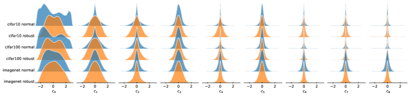
Figure 3: Coefficient distribution along every basis of robust (adversarially-trained) vs. normal models on different datasets. Shifts between robust and normal models appear to decrease with dataset complexity.

4.2 Filter structure

In this section we aim at understanding the differences in the filter structure. For this, we compute a common basis consisting of all collected filters and measure shifts between coefficients separated by dataset and regularization. We weigh the distributions by the explained variance ratio of the respective axis.

Coefficient shifts by dataset

The coefficient distributions (Fig. 3) show clear shifts between robust and normal models, but this shift decreases with increasing complexity of the dataset. We obtain a weighted KL-divergence of 0.55, 0.16, and 0.01 for CIFAR-10/100, and ImageNet1k respectively. Interestingly, we also see a reduced drift for CIFAR-100 compared to CIFAR-10, although it has the same amount of training samples but more classes. This suggests that more complex datasets lead to smaller distribution shifts between robust and normal models, with an emphasis on the fact that complexity does not only refer to the amount of input training data. It is worth noting that robust models achieve a significantly worse clean accuracy than their counterparts and this performance gap increases with dataset complexity (Tab. 1). On average, robust accuracy is an additionally 30% worse for all studied datasets. And ImageNet1k models are evaluated with a different $\epsilon$, which may hide their true (non)-robustness. Additionally, the studied ImageNet1k models on average only employ 2M $3\times 3$ filters (plus a negligible amount of larger filters), while the models on the arguably simpler datasets employ 9M on average. It is therefore likely, that CIFAR-10/100 shows an increased effect of degeneration, and, that ImageNet1k pairs similarity is due to smaller architectures, and lesser robustness performance, rather than intrinsic similarity.

Coefficient shifts by depth

Following the previous observation, we investigate the most significant shifts in filter coefficients and measure the divergence at various stages of depth. To compare models with different depths, we group filter coefficients in deciles of their relative depth in the model. The obtained shifts (Fig. 1) seem to increase with convolution depth and peak in the last 20% of the depth for CIFAR-10/100. For ImageNet1k the peak shift is measured in the 8th decile, whereas the shift in later stages is minimal. Aside of the shifts in later stages, for all datasets, there is relatively low shift throughout the depth with the most salient outlier being seen in the very first convolution layer. This outlier is indeed limited to the first layer, adding filters from the secondary layers vanishes the shift. Once again the maximum shift appears to decrease with dataset complexity.

(a) Adversarial training.

(b) Normal training.

Figure 4: Full set of first stage convolution filters of a WideResNet-34-10 trained with 4(a) adversarial training as provided by [65] on CIFAR-10 and 4(b) normal training.

(a) Adversarial training.

(b) Normal training.

Figure 5: Randomly selected convolution filters of the last convolution layer in a WideResNet-34-10 trained with 5(a) adversarial training as provided by [65] on CIFAR-10 and 5(b) normal training.

First and last convolution layer

To better understand the cause of the observed distribution shifts we visualize the first and last convolution layers. The primary convolution stage (Fig. 4) shows a striking difference: Normal models show an expected [21] diverse set of various filters, yet, almost all robust models develop a large presence of filters performing a weighted summation of the input channels (as $1\times 1$ convolutions would do). We hypothesize that in combination with the common ReLU-activations (and their derivatives) these filters perform a thresholding of the input data which can eliminate small perturbations. Indeed, plotting the difference in activations for natural and perturbed samples ( Fig. 6), allows us to obtain visual confirmation that these filters are successful in removing perturbations from various regions of interest (ROI), e.g. from the cat, background, foreground. For the deepest convolution layers (Fig. 5) we observe the opposite: normal filters show a clear lack of diversity, and mostly remind of gaussian blur filters, while adversarially-trained filters appear to be richer in structure and are more likely to perform complex transformations. Contrary to the distinct primary layer, this observation is visible across multiple deeper layers.

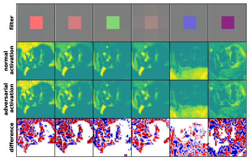
Figure 6: Activations generated by (randomly selected) thresholding-filterbanks (top) in the primary convolution stage of a robust WideResNet-34-10 by [65]. The first row shows the thresholding-filters. The second row shows the activations of each filter for an input sample, and the same sample with perturbations, respectively. Finally, the last row shows the difference in activations: perturbations (red, blue) are removed from ROIs (white).

4.3 Filter quality

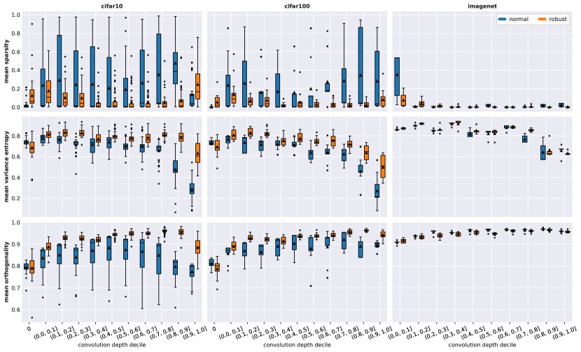
Figure 7: Distribution of filter quality comparison by depth measured via sparsity (top), variance entropy (center), and orthogonality (bottom) between normal and adversarial-training for CIFAR-10 (left), CIFAR-100 (center), ImageNet1k (right) datasets.

While the prevenient analysis focused on distribution shifts in filter structure this section focuses on the related quality aspect of filters. In particular, we measure the amount of contributing filters through sparsity; the diversity of filters through variance entropy; and the redundancy of filterbanks through orthogonality. Similarly to the findings in structure, we observe fewer differences in quality with dataset complexity (Fig. 7), but also a general increase in quality for both robust and normal models. The results on ImageNet1k are less conclusive due to a near-optimal baseline and a low sample size.

Sparsity

We observe a very high span of sparsity across all layers for normal models that decreases with dataset complexity. Robust training significantly further minimizes sparsity and it’s span across all depths. Notable outliers include the primary stages, as well as the deepest convolution layers for CIFAR-10. Generally, sparsity seems to be lower in middle-stages.

Variance entropy

The average variance entropy is relatively constant throughout the model but decreases with deeper layers. The entropy of robust models starts to decrease later and less significantly but the difference between diminishes with dataset complexity. Compared to CIFAR-10, robust CIFAR-100 models shows a lower entropy in deeper layers, while there is no clear difference between normal models. ImageNet1k models show a higher entropy across all depths.

Orthogonality

Robust models show an almost monotonic increase in orthogonality with depth, except for the last decile, whereas normal models eventually begin to decrease in orthogonality. Again the differences diminish with dataset complexity and the span in obtained measurements of non-robust models is crucially increased.

5 Conclusion

Adversarially-trained models appear to learn a particularly more diverse, less redundant, and less sparse set of convolution filters than their non-regularized variants do. We assume that the increase in quality is a response to the additional training strain, as the more challenging adversarial problem occupies more of the available model capacity that would otherwise be degenerated. We observe a similar effect during normal training with increasing dataset complexity. However, although the filter quality of normally trained ImageNet1k models is exceptionally high, their robustness is not. So, filter quality alone is not a sufficient criterion to establish robustness. We end with the following currently unanswered questions: Is dataset complexity the cause for lower quality shifts, or, is the difference we measure merely a side effect of heavily overparameterized architectures in which adversarial training can close the gap to more complex datasets? If not, can we increase robustness by filter quality regularization during training?

References

- [1] Christian Szegedy, Wojciech Zaremba, Ilya Sutskever, Joan Bruna, Dumitru Erhan, Ian Goodfellow, and Rob Fergus, “Intriguing properties of neural networks,” arXiv, Dec 2013.
- [2] Seyed-Mohsen Moosavi-Dezfooli, Alhussein Fawzi, and Pascal Frossard, “DeepFool: a simple and accurate method to fool deep neural networks,” arXiv, Nov 2015.
- [3] Xingjun Ma, Yuhao Niu, Lin Gu, Yisen Wang, Yitian Zhao, James Bailey, and Feng Lu, “Understanding adversarial attacks on deep learning based medical image analysis systems,” Pattern Recognition, vol. 110, p. 107332, 2021.
- [4] Samuel G. Finlayson, John D. Bowers, Joichi Ito, Jonathan L. Zittrain, Andrew L. Beam, and Isaac S. Kohane, “Adversarial attacks on medical machine learning,” Science, vol. 363, no. 6433, pp. 1287–1289, 2019.
- [5] Yao Deng, Xi Zheng, Tianyi Zhang, Chen Chen, Guannan Lou, and Miryung Kim, “An analysis of adversarial attacks and defenses on autonomous driving models,” 2020.
- [6] Nicholas Carlini and David Wagner, “Towards Evaluating the Robustness of Neural Networks,” arXiv, Aug 2016.
- [7] Naveed Akhtar and Ajmal Mian, “Threat of adversarial attacks on deep learning in computer vision: A survey,” Ieee Access, vol. 6, pp. 14410–14430, 2018.
- [8] Nicolas Papernot, Patrick McDaniel, Xi Wu, Somesh Jha, and Ananthram Swami, “Distillation as a Defense to Adversarial Perturbations against Deep Neural Networks,” arXiv, Nov 2015.
- [9] Ian J. Goodfellow, Jonathon Shlens, and Christian Szegedy, “Explaining and Harnessing Adversarial Examples,” arXiv, Dec 2014.
- [10] Aleksander Madry, Aleksandar Makelov, Ludwig Schmidt, Dimitris Tsipras, and Adrian Vladu, “Towards deep learning models resistant to adversarial attacks,” in International Conference on Learning Representations, 2018.
- [11] Ali Shafahi, Mahyar Najibi, Amin Ghiasi, Zheng Xu, John Dickerson, Christoph Studer, Larry S. Davis, Gavin Taylor, and Tom Goldstein, “Adversarial Training for Free!,” arXiv, Apr 2019.
- [12] Alex Krizhevsky, “Learning multiple layers of features from tiny images,” tech. rep., 2009.
- [13] Olga Russakovsky, Jia Deng, Hao Su, Jonathan Krause, Sanjeev Satheesh, Sean Ma, Zhiheng Huang, Andrej Karpathy, Aditya Khosla, Michael Bernstein, Alexander C. Berg, and Li Fei-Fei, “ImageNet Large Scale Visual Recognition Challenge,” International Journal of Computer Vision (IJCV), vol. 115, no. 3, pp. 211–252, 2015.
- [14] Paul Gavrikov and Janis Keuper, “CNN-Filter-DB-Robust v1.0.0,” June 2022. Distributed by Zenodo. doi: https://doi.org/10.5281/zenodo.6414075.
- [15] Yair Carmon, Aditi Raghunathan, Ludwig Schmidt, Percy Liang, and John C. Duchi, “Unlabeled data improves adversarial robustness,” 2022.
- [16] Francesco Croce, Maksym Andriushchenko, Vikash Sehwag, Edoardo Debenedetti, Nicolas Flammarion, Mung Chiang, Prateek Mittal, and Matthias Hein, “RobustBench: a standardized adversarial robustness benchmark,” in Thirty-fifth Conference on Neural Information Processing Systems Datasets and Benchmarks Track, 2021.
- [17] Francesco Croce and Matthias Hein, “Reliable evaluation of adversarial robustness with an ensemble of diverse parameter-free attacks,” in ICML, 2020.
- [18] Francesco Croce and Matthias Hein, “Minimally distorted adversarial examples with a fast adaptive boundary attack,” 2020.
- [19] Maksym Andriushchenko, Francesco Croce, Nicolas Flammarion, and Matthias Hein, “Square attack: A query-efficient black-box adversarial attack via random search,” in Computer Vision – ECCV 2020 (Andrea Vedaldi, Horst Bischof, Thomas Brox, and Jan-Michael Frahm, eds.), (Cham), pp. 484–501, Springer International Publishing, 2020.
- [20] Peter Lorenz, Dominik Strassel, Margret Keuper, and Janis Keuper, “Is robustbench/autoattack a suitable benchmark for adversarial robustness?,” in The AAAI-22 Workshop on Adversarial Machine Learning and Beyond, 2022.
- [21] Jason Yosinski, Jeff Clune, Yoshua Bengio, and Hod Lipson, “How transferable are features in deep neural networks?,” vol. 4, 2014.
- [22] Christian Szegedy, Wei Liu, Yangqing Jia, Pierre Sermanet, Scott Reed, Dragomir Anguelov, Dumitru Erhan, Vincent Vanhoucke, and Andrew Rabinovich, “Going deeper with convolutions,” 2014.
- [23] Chris Olah, Nick Cammarata, Ludwig Schubert, Gabriel Goh, Michael Petrov, and Shan Carter, “Zoom in: An introduction to circuits,” Distill, vol. 5, 2020.
- [24] Chris Olah, Nick Cammarata, Ludwig Schubert, Gabriel Goh, Michael Petrov, and Shan Carter, “An overview of early vision in inceptionv1,” Distill, 2020. https://distill.pub/2020/circuits/early-vision.
- [25] Nick Cammarata, Gabriel Goh, Shan Carter, Ludwig Schubert, Michael Petrov, and Chris Olah, “Curve detectors,” Distill, 2020. https://distill.pub/2020/circuits/curve-detectors.
- [26] Chris Olah, Nick Cammarata, Chelsea Voss, Ludwig Schubert, and Gabriel Goh, “Naturally occurring equivariance in neural networks,” Distill, 2020. https://distill.pub/2020/circuits/equivariance.
- [27] Ludwig Schubert, Chelsea Voss, Nick Cammarata, Gabriel Goh, and Chris Olah, “High-low frequency detectors,” Distill, 2021. https://distill.pub/2020/circuits/frequency-edges.
- [28] Nick Cammarata, Gabriel Goh, Shan Carter, Chelsea Voss, Ludwig Schubert, and Chris Olah, “Curve circuits,” Distill, 2021. https://distill.pub/2020/circuits/curve-circuits.
- [29] Chelsea Voss, Nick Cammarata, Gabriel Goh, Michael Petrov, Ludwig Schubert, Ben Egan, Swee Kiat Lim, and Chris Olah, “Visualizing weights,” Distill, 2021. https://distill.pub/2020/circuits/visualizing-weights.
- [30] Chelsea Voss, Gabriel Goh, Nick Cammarata, Michael Petrov, Ludwig Schubert, and Chris Olah, “Branch specialization,” Distill, 2021. https://distill.pub/2020/circuits/branch-specialization.
- [31] Michael Petrov, Chelsea Voss, Ludwig Schubert, Nick Cammarata, Gabriel Goh, and Chris Olah, “Weight banding,” Distill, 2021. https://distill.pub/2020/circuits/weight-banding.
- [32] Paul Gavrikov and Janis Keuper, “Cnn filter db: An empirical investigation of trained convolutional filters,” in 2022 IEEE/CVF Conference on Computer Vision and Pattern Recognition (CVPR), 2022.
- [33] Jonathan Frankle and Michael Carbin, “The lottery ticket hypothesis: Finding sparse, trainable neural networks,” arXiv preprint arXiv:1803.03635, 2018.
- [34] Yang Bai, Yuyuan Zeng, Yong Jiang, Shu-Tao Xia, Xingjun Ma, and Yisen Wang, “Improving adversarial robustness via channel-wise activation suppressing,” in International Conference on Learning Representations, 2021.
- [35] Yong Guo, David Stutz, and Bernt Schiele, “Improving corruption and adversarial robustness by enhancing weak subnets,” 2022.
- [36] Francisco Utrera, Evan Kravitz, N. Benjamin Erichson, Rajiv Khanna, and Michael W. Mahoney, “Adversarially-trained deep nets transfer better: Illustration on image classification,” in International Conference on Learning Representations, 2021.
- [37] I Jolliffe, Principal Component Analysis. New York, NY: Springer New York, 1986.
- [38] Andrew Brock, Theodore Lim, J. M. Ritchie, and Nick Weston, “Neural photo editing with introspective adversarial networks,” 2017.
- [39] Andrew Brock, Jeff Donahue, and Karen Simonyan, “Large scale GAN training for high fidelity natural image synthesis,” in International Conference on Learning Representations, 2019.
- [40] S. Kullback and R. A. Leibler, “On Information and Sufficiency,” The Annals of Mathematical Statistics, vol. 22, no. 1, pp. 79 – 86, 1951.
- [41] Sylvestre-Alvise Rebuffi, Sven Gowal, Dan A. Calian, Florian Stimberg, Olivia Wiles, and Timothy Mann, “Fixing data augmentation to improve adversarial robustness,” 2021.
- [42] Hanxun Huang, Yisen Wang, Sarah Monazam Erfani, Quanquan Gu, James Bailey, and Xingjun Ma, “Exploring architectural ingredients of adversarially robust deep neural networks,” 2022.
- [43] Jingfeng Zhang, Xilie Xu, Bo Han, Gang Niu, Lizhen Cui, Masashi Sugiyama, and Mohan Kankanhalli, “Attacks which do not kill training make adversarial learning stronger,” 2020.
- [44] Dinghuai Zhang, Tianyuan Zhang, Yiping Lu, Zhanxing Zhu, and Bin Dong, “You only propagate once: Accelerating adversarial training via maximal principle,” 2019.
- [45] Dan Hendrycks, Kimin Lee, and Mantas Mazeika, “Using pre-training can improve model robustness and uncertainty,” 2019.
- [46] Jingfeng Zhang, Jianing Zhu, Gang Niu, Bo Han, Masashi Sugiyama, and Mohan Kankanhalli, “Geometry-aware instance-reweighted adversarial training,” 2021.
- [47] Erh-Chung Chen and Che-Rung Lee, “Ltd: Low temperature distillation for robust adversarial training,” 2021.
- [48] Maksym Andriushchenko and Nicolas Flammarion, “Understanding and improving fast adversarial training,” 2020.
- [49] Jiequan Cui, Shu Liu, Liwei Wang, and Jiaya Jia, “Learnable boundary guided adversarial training,” 2021.
- [50] Leslie Rice, Eric Wong, and J. Zico Kolter, “Overfitting in adversarially robust deep learning,” 2020.
- [51] Sihui Dai, Saeed Mahloujifar, and Prateek Mittal, “Parameterizing activation functions for adversarial robustness,” 2021.
- [52] Sven Gowal, Chongli Qin, Jonathan Uesato, Timothy Mann, and Pushmeet Kohli, “Uncovering the limits of adversarial training against norm-bounded adversarial examples,” 2021.
- [53] Chawin Sitawarin, Supriyo Chakraborty, and David Wagner, “Sat: Improving adversarial training via curriculum-based loss smoothing,” 2021.
- [54] Jinghui Chen, Yu Cheng, Zhe Gan, Quanquan Gu, and Jingjing Liu, “Efficient robust training via backward smoothing,” 2021.
- [55] Hongyang Zhang, Yaodong Yu, Jiantao Jiao, Eric P. Xing, Laurent El Ghaoui, and Michael I. Jordan, “Theoretically principled trade-off between robustness and accuracy,” 2019.
- [56] Dongxian Wu, Shu tao Xia, and Yisen Wang, “Adversarial weight perturbation helps robust generalization,” 2020.
- [57] Eric Wong, Leslie Rice, and J. Zico Kolter, “Fast is better than free: Revisiting adversarial training,” 2020.
- [58] Lang Huang, Chao Zhang, and Hongyang Zhang, “Self-adaptive training: beyond empirical risk minimization,” 2020.
- [59] Tianyu Pang, Xiao Yang, Yinpeng Dong, Kun Xu, Jun Zhu, and Hang Su, “Boosting adversarial training with hypersphere embedding,” 2020.
- [60] Sven Gowal, Sylvestre-Alvise Rebuffi, Olivia Wiles, Florian Stimberg, Dan Andrei Calian, and Timothy Mann, “Improving robustness using generated data,” 2021.
- [61] Vikash Sehwag, Shiqi Wang, Prateek Mittal, and Suman Jana, “Hydra: Pruning adversarially robust neural networks,” 2020.
- [62] Kaustubh Sridhar, Oleg Sokolsky, Insup Lee, and James Weimer, “Improving neural network robustness via persistency of excitation,” 2021.
- [63] Tianlong Chen, Sijia Liu, Shiyu Chang, Yu Cheng, Lisa Amini, and Zhangyang Wang, “Adversarial robustness: From self-supervised pre-training to fine-tuning,” 2020.
- [64] Vikash Sehwag, Saeed Mahloujifar, Tinashe Handina, Sihui Dai, Chong Xiang, Mung Chiang, and Prateek Mittal, “Robust learning meets generative models: Can proxy distributions improve adversarial robustness?,” 2021.
- [65] Sravanti Addepalli, Samyak Jain, Gaurang Sriramanan, Shivangi Khare, and Venkatesh Babu Radhakrishnan, “Towards achieving adversarial robustness beyond perceptual limits,” in ICML 2021 Workshop on Adversarial Machine Learning, 2021.
- [66] Gavin Weiguang Ding, Yash Sharma, Kry Yik Chau Lui, and Ruitong Huang, “Mma training: Direct input space margin maximization through adversarial training,” in International Conference on Learning Representations, 2020.
- [67] Rahul Rade and Seyed-Mohsen Moosavi-Dezfooli, “Helper-based adversarial training: Reducing excessive margin to achieve a better accuracy vs. robustness trade-off,” in ICML 2021 Workshop on Adversarial Machine Learning, 2021.
- [68] Yisen Wang, Difan Zou, Jinfeng Yi, James Bailey, Xingjun Ma, and Quanquan Gu, “Improving adversarial robustness requires revisiting misclassified examples,” in International Conference on Learning Representations, 2020.
- [69] Logan Engstrom, Andrew Ilyas, Hadi Salman, Shibani Santurkar, and Dimitris Tsipras, “Robustness (python library),” 2019.
- [70] Ross Wightman, “Pytorch image models.” https://github.com/rwightman/pytorch-image-models, 2019.