$\mathcal{R}^{2}$ Quantum Corrected Scalar Field Inflation

Abstract

String theory enjoys an elevated role among quantum gravity theories, since it seems to be the most consistent UV completion of general relativity and the Standard Model. However, it is hard to verify the existence of this underlying theory on terrestrial accelerators. One way to probe string theory is to study its imprints on the low-energy effective inflationary Lagrangian, which are quantified in terms of high energy correction terms. It is highly likely, thus, to find higher order curvature terms combined with string moduli, that is scalar fields, since both these types of interactions and matter fields appear in string theory. In this work we aim to stress the probability that the inflationary dynamics are controlled by the synergy of scalar fields and higher order curvature terms. Specifically, we shall consider a well motivated quantum corrected canonical scalar field theory, with the quantum corrections being of the $\mathcal{R}^{2}$ type. The reason for choosing minimally coupled scalar theory is basically because if scalar fields are evaluated in their vacuum configuration, they will either be minimally coupled or conformally coupled. Here we choose the former case, and the whole study shall be performed in the string frame (Jordan frame), in contrast to similar studies in the literature where the Einstein frame two scalar theory is considered. We derive the field equations of the quantum-corrected theory at leading order and we present the form the slow-roll indices obtain for the quantum corrected theory. We exemplify our theoretical framework by using the quadratic inflation model, and as we show, the $\mathcal{R}^{2}$ quantum corrected quadratic inflation model produces a viable inflationary phenomenology, in contrast with the simple quadratic inflation model.

I Introduction

String theory is to date the most successful candidate for describing the pre-inflationary quantum state of the Universe, since it unifies gravity with the Standard Model fundamental interactions in a consistent way. However, the drawback of this theory is that the predictions of it cannot be tested for the moment on terrestrial particle accelerators. The LHC has achieved a 15 TeV center of mass energy scale and no sign of alternative to the Standard Model physics seems to exist. Even supersymmetry does not seem to exist for scales up to 15 TeV center of mass thus, for the moment, high energy physics are not directly linked to the world we can access experimentally. This however is not a problem of string theory, it is our problem since we need to find alternative ways to test high energy physics realistically in the world we access. One consistent and elegant way to obtain hints on high energy physics works, is to try to find traces of the high energy physics Lagrangian, to the low energy effective Lagrangian which describes the Universe in the early stages of its classical evolution. To date, it is believed that the Universe after the quantum epoch entered the inflationary era inflation1 ; inflation2 ; inflation3 ; inflation4 , during which the Universe is theorized to be classical and four dimensional. But as we mentioned, it is quite possible to find high energy physics traces in the inflationary Lagrangian, in the form of quantum corrections. This possibility is sensational since it will provide insights that, for the moment, are hard to obtain from terrestrial accelerators. Inflation and early-time cosmology will be tested in the following two decades, and the scientific community hopes that some light will eventually be shed on the early-time physics and strong answers will be given on the question of how our Universe works. There are two ways to test the early-time era, and both of these aim to the sky and do not rely on terrestrial particle accelerators. The first way is to seek traces of inflation originating patterns in the Cosmic Microwave Background (CMB) temperature fluctuations. The future experiments which are basically the fourth generation CMB experiments CMB-S4:2016ple ; SimonsObservatory:2019qwx , will seek for the $B$-modes of inflation (curl mode) Kamionkowski:2015yta . It is known that $B$-modes can be generated in two ways, from the gravitational lensing generated transition of $E$-modes to $B$-modes at small angular scales or equivalently large multipoles of the CMB, or from primordial tensor modes, the so called primordial gravitational waves, at large angular scales or equivalently low multipoles of the CMB. Thus the CMB-based way to detect primordial gravitational wave generated patterns on the CMB, is to look at the low multipoles of the CMB. The other way to probe the post-quantum era of our Universe, is more direct than the CMB way, and it will be based on future space high frequency interferometers Hild:2010id ; Baker:2019nia ; Smith:2019wny ; Crowder:2005nr ; Smith:2016jqs ; Seto:2001qf ; Kawamura:2020pcg ; Bull:2018lat . These interferometers will seek directly for a stochastic background of primordial gravitational waves. This observation will be sensational to say the least, and will stir things up significantly in both high energy physics and theoretical cosmology.

Most of the inflationary theories use the single scalar field description, which is simple to tackle analytically. But as we mentioned, it is highly likely that the string theory era will have its effect on the low-energy effective inflationary Lagrangian. These low-energy string oriented effects come in terms of higher order curvature corrections Codello:2015mba . Therefore, it is possible that not just a single scalar field controls the dynamics of inflation, but the synergy of a scalar field and the higher order curvature terms as part of some modified gravity terms reviews1 ; reviews2 ; reviews3 ; reviews4 ; reviews5 ; reviews6 , might actually control the inflationary era. This issue started to appear in the recent literature of theoretical cosmology Ema:2017rqn ; Ema:2020evi ; Ivanov:2021ily ; Gottlober:1993hp ; delaCruz-Dombriz:2016bjj ; Enckell:2018uic ; Karam:2018mft ; Kubo:2020fdd ; Gorbunov:2018llf ; Calmet:2016fsr ; Oikonomou:2021msx , and it is not simply an academic exercise, but might be a compelling task in the future. The motivation for using combined scalar field and higher order gravity Lagrangians is apparent, both scalar fields (string moduli) and higher order gravity terms originate from the underlying string theory. Thus, one must include both these ingredients in the low-energy Lagrangian in order to be accurate and scientifically ”democratic” towards treating the higher order fields and terms. Single field approaches and pure modified gravity terms are simpler to treat analytically, but this is not a compelling motivation to exclude the probability of finding combined effects in the inflationary Lagrangian. Another motivation comes from the fact that non-tachyon single scalar field theories and fundamental modified gravity theories, like for example $f(\mathcal{R})$ gravity, seem to predict a significantly low energy spectrum of primordial gravitational waves. Thus, if a future direct signal of stochastic gravitational waves is detected, this will certainly exclude these descriptions, unless some exotic scenario occurs, which however must enhance the spectrum $10^{4}-10^{8}$ times in order to be detected. Thus combinations of single scalar field descriptions with modified gravity terms seem to be an elegant possibility, since in these theories, significant enhancement of the primordial gravitational wave energy spectrum might occur, see for example Ref. Odintsov:2021kup . When the scalar field is evaluated in its vacuum configuration, it either is minimally coupled or conformally coupled, and thus the quantum corrections will either appear in conformally coupled single scalar field Lagrangians, or minimally coupled scalar field Lagrangians. In most works appearing to date in the literature, the first perspective is studied, where the inflationary phenomenology of the Higgs scalar is considered in the presence of $\mathcal{R}^{2}$ quantum corrections Ema:2017rqn ; Ema:2020evi ; Ivanov:2021ily ; Gottlober:1993hp ; delaCruz-Dombriz:2016bjj ; Enckell:2018uic ; Karam:2018mft ; Kubo:2020fdd ; Gorbunov:2018llf ; Calmet:2016fsr . However, all the existing approaches study the inflationary phenomenology in the Einstein frame, thus the resulting theory has effectively two scalar fields. There is another possibility though, to investigate the phenomenology of these combined scalar field-modified gravity theories in the string frame (Jordan frame). This perspective was investigated for power-law $f(\mathcal{R})\sim\mathcal{R}^{n}$ gravity in Oikonomou:2021msx , however the most important quantum correction, the $\mathcal{R}^{2}$ was not studied, since it could not be derived formally for the general $n$ case. This is due to the fact that for $n=2$ the situation is much more simple and more easy to tackle analytically, than the general $\mathcal{R}^{n}$ case. In this paper we shall study minimally coupled single scalar field theory in the presence of $\mathcal{R}^{2}$ quantum corrections in the string frame. We shall derive the field equations, and by using the slow-roll assumptions, and physically motivated assumptions, we shall quantify the effect of the $\mathcal{R}^{2}$ quantum corrections on single scalar field inflation. The resulting effective field equations acquire an elegant final form as we will demonstrate, and accordingly the inflationary phenomenology of the resulting theory will thoroughly be investigated.

This work is organized as follows: In section II we shall present the general $\mathcal{R}^{2}$ quantum corrected single field Lagrangian and field equations. We quantify the leading order $\mathcal{R}^{2}$ quantum corrections in the field equations, and we express the slow-roll indices and the corresponding observational indices in terms of the scalar field, in which the $\mathcal{R}^{2}$ quantum effects are included. In section III we analyze in depth one example model which yields a viable inflationary era compatible with the latest CMB constraints on inflation. Finally, the conclusions follow in the end of the paper.

II Canonical Scalar Field Inflation in the presence of $R^{2}$ Gravity: Formalism

The most general four dimensional scalar field Lagrangian containing at most two derivatives is,

$$\mathcal{S}_{\varphi}=\int\mathrm{d}^{4}x\sqrt{-g}\left(\frac{1}{2}Z(\varphi)g^{\mu\nu}\partial_{\mu}\varphi\partial_{\nu}\varphi+\mathcal{V}(\varphi)+h(\varphi)\mathcal{R}\right)\,,$$ (1)

and when the scalar fields are evaluated at their vacuum configuration, the scalar field must be either minimally coupled of conformally coupled. We shall focus on the first possibility in which $Z(\varphi)=-1$ and $h(\varphi)=1$ in the action (1). Now the quantum corrections local effective action which is consistent with diffeomorphism invariance and contains up to fourth order derivatives, is Codello:2015mba ,

$$\mathcal{S}_{eff}=\int\mathrm{d}^{4}x\sqrt{-g}\Big{(}\Lambda_{1}+\Lambda_{2}\mathcal{R}+\Lambda_{3}\mathcal{R}^{2}+\Lambda_{4}\mathcal{R}_{\mu\nu}\mathcal{R}^{\mu\nu}+\Lambda_{5}\mathcal{R}_{\mu\nu\alpha\beta}\mathcal{R}^{\mu\nu\alpha\beta}+\Lambda_{6}\square\mathcal{R}$$ (2)

$$+\Lambda_{7}\mathcal{R}\square\mathcal{R}+\Lambda_{8}\mathcal{R}_{\mu\nu}\square\mathcal{R}^{\mu\nu}+\Lambda_{9}\mathcal{R}^{3}+\mathcal{O}(\partial^{8})+...\Big{)}\,,$$

where the parameters $\Lambda_{i}$, $i=1,2,...,6$ are appropriate dimensionful constants. Also non-analytical “leading logs” correction terms of the form $\mathcal{R}^{2}\log\mathcal{R}$ might be present and also non-local terms $\mathcal{R}\log\frac{-\square\mathcal{R}}{\mu^{2}}$, the phenomenology of which was analyzed in Odintsov:2017hbk . In this paper, we shall focus on the $\mathcal{R}^{2}$ corrections, which is among the simplest corrections one can consider. Thus, the minimally coupled single scalar field action including the $\mathcal{R}^{2}$ corrections is effectively an $f(\mathcal{R},\varphi)$ action of the form,

$$\centering\mathcal{S}=\int{d^{4}x\sqrt{-g}\left(\frac{f(\mathcal{R})}{2\kappa^{2}}-\frac{1}{2}g^{\mu\nu}\partial_{\mu}\varphi\partial_{\nu}\varphi-\mathcal{V}(\varphi)\right)}\,,\@add@centering$$ (3)

where $\kappa^{2}=8\pi G=\frac{1}{Mp^{2}}$ and $M_{p}$ stands for the reduced Planck mass, and also,

$$f(\mathcal{R})=\mathcal{R}+\frac{\mathcal{R}^{2}}{36M^{2}}\,,$$ (4)

with $M$ being a mass scale to be determined later on. Note that, since the model we are considering is an $f(\mathcal{R},\varphi)$ theory in the string frame, the value of $M$ is not required to be that of the standard $\mathcal{R}^{2}$ model Starobinsky:1980te ; Bezrukov:2007ep , and it will generally take different values from the usual ones obtained by phenomenological reasons for the vacuum $\mathcal{R}^{2}$ model in the Einstein frame Appleby:2009uf . For the background metric, we assume a flat Friedmann-Robertson-Walker (FRW) metric with line element,

$$\centering\mathrm{d}s^{2}=-\mathrm{d}t^{2}+a(t)\sum_{i=1}^{3}\mathrm{d}x_{i}^{2},\@add@centering$$ (5)

with $\alpha(t)$ being the scale factor and the corresponding Hubble rate is $\mathcal{H}=\frac{\dot{a}}{a}$. Upon varying the gravitational action (3) with respect to the metric, we obtain the following field equations,

$$3f_{\mathcal{R}}\mathcal{H}^{2}=\frac{Rf_{\mathcal{R}}-f}{2}-3\mathcal{H}\dot{F}_{\mathcal{R}}+\kappa^{2}\big{(}\frac{1}{2}\dot{\varphi}^{2}+\mathcal{V}(\varphi)\big{)}\ ,$$ (6)

$$-2f_{\mathcal{R}}\dot{\mathcal{H}}=\kappa^{2}\dot{\varphi}^{2}+\ddot{f}_{\mathcal{R}}-\mathcal{H}\dot{f}_{\mathcal{R}}\ ,$$ (7)

$$\ddot{\varphi}+3\mathcal{H}\dot{\varphi}+\mathcal{V}^{\prime}=0\ ,$$ (8)

where the “dot” denotes the derivative with respect to cosmic time, the “prime” describes derivative with respect to the scalar field $\varphi$ and $f_{\mathcal{R}}=\frac{\partial f}{\partial\mathcal{R}}$. Taking into consideration that $f(\mathcal{R})=\mathcal{R}+\frac{\mathcal{R}^{2}}{36M^{2}}$ and also that the Ricci scalar and its derivative for the FRW are given by,

$$\mathcal{R}=12\mathcal{H}^{2}+6\dot{\mathcal{H}}\,,\ \dot{\mathcal{R}}=24\mathcal{H}\dot{\mathcal{H}}+6\ddot{\mathcal{H}},$$ (9)

the Friedmann and Raychaudhuri equations become,

$$3\mathcal{H}^{2}+\frac{3}{M^{2}}\mathcal{H}^{2}\dot{\mathcal{H}}=\frac{\dot{\mathcal{H}}^{2}}{2}-\frac{\ddot{\mathcal{H}}\mathcal{H}}{M^{2}}+\kappa^{2}\big{(}\frac{1}{2}\dot{\varphi}^{2}+\mathcal{V}(\varphi)\big{)},$$ (10)

$$-2\dot{\mathcal{H}}-\frac{2}{M^{2}}\dot{\mathcal{H}}^{2}=-\frac{\ddot{\mathcal{H}}\mathcal{H}}{M^{2}}+\kappa^{2}\dot{\varphi}^{2},$$ (11)

with a remarkable cancellation of the terms $\mathcal{H}^{2}\dot{\mathcal{H}}$ taking place in the latter one, which is absent in the case that a power-law $\mathcal{R}^{n}$ gravity is considered, with $n\neq 2$, see Oikonomou:2021msx . The slow-roll conditions during the inflationary era demand that,

$$\dot{\mathcal{H}}\ll\mathcal{H}^{2}\ ,\ \ddot{\mathcal{H}}\ll\mathcal{H}\dot{\mathcal{H}},$$ (12)

however the term $\frac{\mathcal{H}^{2}\dot{\mathcal{H}}}{M^{2}}$ is possibly of the same order as $\mathcal{H}^{2}$, at least for a quasi-de Sitter evolution. Thus, we can easily neglect the terms containing the higher order Hubble rate derivative $\sim\ddot{\mathcal{H}}$ and we shall also assume that the following approximations hold true,

$$\frac{\dot{\mathcal{H}}^{2}}{M^{2}}\ll\mathcal{H}^{2},\,\,\,\frac{\dot{\mathcal{H}}^{2}}{M^{2}}\ll\mathcal{V}(\varphi)\,.$$ (13)

Although the above approximations are well justified for a usual quasi-de Sitter evolution, it is compelling to examine that these hold true for a viable inflationary phenomenology, for the same values of the free parameters which guarantee the viability of the model. Moreover, in the same fashion as single scalar field inflation, we will require the scalar field to satisfy,

$$\frac{1}{2}\dot{\varphi}^{2}\ll\mathcal{V}(\varphi)\ ,\ \ddot{\varphi}\ll\mathcal{H}\dot{\varphi}.$$ (14)

In effect of all the above, the field equations take the form,

$$3\mathcal{H}^{2}+\frac{3\mathcal{H}^{2}}{M^{2}}\dot{\mathcal{H}}\simeq\kappa^{2}\mathcal{V}(\varphi),$$ (15)

$$-2\dot{\mathcal{H}}-\frac{2}{M^{2}}\dot{\mathcal{H}}^{2}\simeq\kappa^{2}\dot{\varphi}^{2},$$ (16)

$$\dot{\varphi}\simeq-\frac{\mathcal{V}^{\prime}}{3\mathcal{H}}.$$ (17)

We notice that the Raychaudhuri equation is practically a second order polynomial equation with respect to $\dot{\mathcal{H}}$, thus the solution is,

$$\dot{\mathcal{H}}=\frac{-M^{2}+M\sqrt{M^{2}-2\dot{\varphi}^{2}\kappa^{2}}}{2}\,,$$ (18)

and the Friedmann equation becomes,

$$\frac{3\mathcal{H}^{2}}{2}-\frac{3\mathcal{H}^{2}\sqrt{M^{2}-2\dot{\varphi}^{2}\kappa^{2}}}{2M}\simeq\kappa^{2}\mathcal{V}(\varphi)\,.$$ (19)

In the following we shall use the approximation,

$$\frac{2\kappa^{2}\dot{\varphi}^{2}}{M^{2}}\ll 1\,,$$ (20)

The validity of the approximations (13) and (20) must be tested for any potential viable inflationary model. As long as the above approximation holds true, the Friedmann and Raychaudhuri equations acquire the following form at leading order,

$$\mathcal{H}^{2}\simeq\frac{\kappa^{2}\mathcal{V}(\varphi)}{3}+\mathcal{O}(\frac{\kappa^{2}\dot{\varphi}^{2}}{2}\mathcal{H}^{2}),$$ (21)

$$\dot{\mathcal{H}}\simeq-\frac{\kappa^{2}\dot{\varphi}^{2}}{2}-\frac{\kappa^{4}\dot{\varphi}^{4}}{4M^{2}}\,.$$ (22)

The resulting equations of motion, namely Eqs. (21), (22) and the slow-roll scalar field equation, namely Eq. (17) will be the starting point of our analysis. Basically these equations depict the direct effect of the $R^{2}$ corrections on the standard scalar field inflation in the Jordan frame. The second term in the Raychaudhuri equation is basically a quantum correction in the field equations introduced by the presence of the $\mathcal{R}^{2}$ quantum corrections in the effective inflationary Lagrangian, when of course the condition (20) holds true. The effects of the $\mathcal{R}^{2}$ gravity term are quantified in the Raychaudhuri equation (22), and will also affect crucially the slow-roll indices. The slow-roll indices for a general $f(\mathcal{R},\varphi)$ theory are defined Hwang:2005hb ,

$$\epsilon_{1}=-\frac{\dot{\mathcal{H}}}{\mathcal{H}^{2}},\,\,\,\epsilon_{2}=\frac{\ddot{\varphi}}{\mathcal{H}\dot{\varphi}},\,\,\,\epsilon_{3}=\frac{\dot{f}_{\mathcal{R}}}{2\mathcal{H}f_{\mathcal{R}}},\,\,\,\epsilon_{4}=\frac{\dot{E}}{2\mathcal{H}E}\,,$$ (23)

where,

$$E=f_{\mathcal{R}}+\frac{3\dot{f}_{\mathcal{R}}^{2}}{3\kappa^{2}\dot{\varphi}^{2}}\,.$$ (25)

Using the equations (21) and (22), the first slow-roll index $\epsilon_{1}$ is easily found equal to,

$$\epsilon_{1}=\frac{1}{2\kappa^{2}}\left(\left(\frac{\mathcal{V}^{\prime}}{V}\right)^{2}+\frac{1}{6M^{2}}{\left(\frac{\mathcal{V}^{\prime}}{V}\right)}^{2}\frac{\mathcal{V}^{\prime 2}}{V}\right)\,.$$ (26)

As for the expression of $\epsilon_{2}$ we also use (17), from which we calculate $\ddot{\varphi}$, so after some algebra, the second slow-roll index reads,

$$\epsilon_{2}=-\frac{\mathcal{V}^{\prime\prime}}{\kappa^{2}V}+\epsilon_{1}\,.$$ (27)

Also the resulting expression for the slow-roll index $\epsilon_{3}$ yields,

$$\epsilon_{3}=\frac{\epsilon_{1}}{-1-\frac{3M^{2}}{2\mathcal{H}^{2}}+\frac{\epsilon_{1}}{2}}\,.$$ (28)

The expression of $\epsilon_{4}$ is the most complex one so far. We firstly calculate $E$ and $\dot{E}$,

$$E=1+\frac{2\mathcal{R}}{36M^{2}}+\frac{8}{3\kappa^{2}M^{4}}\frac{\mathcal{H}^{2}\dot{\mathcal{H}}^{2}}{\dot{\varphi}^{2}},$$ (29)

$$\dot{E}=\frac{4\mathcal{H}\dot{\mathcal{H}}}{3M^{2}}+\frac{16}{3\kappa^{2}M^{4}\dot{\varphi}^{4}}\big{(}\mathcal{H}\dot{\mathcal{H}}^{3}\dot{\varphi}^{2}-\mathcal{H}^{2}\dot{\mathcal{H}}^{2}\dot{\varphi}\ddot{\varphi}\big{)},$$ (30)

thus, the full expression of $\epsilon_{4}$ can be obtained by substituting (29), (30) to $\epsilon_{4}$ in (23). Therefore, the dynamical evolution of the inflationary era for the $\mathcal{R}^{2}$ quantum corrected minimally coupled canonical scalar field theory is described by Eqs. (26)-(30), in which the effects of the $\mathcal{R}^{2}$ terms are clearly seen. This will be the starting point for studying the inflationary phenomenology of a scalar field model with an arbitrary scalar potential.

Let us move on to the calculation of the spectral index of the primordial scalar curvature perturbations, the tensor-to-scalar ratio and the tensor spectral index. In the case of a slow-roll expansion, for which the slow-roll indices satisfy $\dot{\epsilon}_{i}\ll 1$, $i=1,2,3,4$, the scalar spectral index is written in terms of the slow-roll indices as Hwang:2005hb ,

$$n_{\mathcal{S}}=1-\frac{4\epsilon_{1}+2\epsilon_{2}-2\epsilon_{3}+2\epsilon_{4}}{1-\epsilon_{1}}.$$ (31)

Now, the ratio of the tensor power spectrum over the scalar one for a general $f(R,\varphi)$ theory is given by Hwang:2005hb ,

$$r=16(\epsilon_{1}+\epsilon_{3}),$$ (32)

and this is the one we will use in our analysis hereafter. Finally, the tensor spectral index is,

$$n_{\mathcal{T}}\sim-2(\epsilon_{1}+\epsilon_{3})\,.$$ (33)

Using Eqs. (31)-(33), the phenomenology of an arbitrary model can directly be tested. Finally, the expression that gives the e-foldings number is,

$$N=\int_{t_{i}}^{t_{f}}\mathcal{H}dt=\int_{\varphi_{i}}^{\varphi_{f}}\frac{\mathcal{H}}{\dot{\varphi}}d\varphi,$$ (34)

where $t_{i}$ and $\varphi_{i}$ are the time instance marking the beginning of the inflation and the value of the scalar field at this point respectively, while $t_{f}$ and $\varphi_{f}$ are the corresponding values at the end of the inflationary era. Using Eqs. (21) and (17), the $e$-foldings number takes the following form,

$$N=\int_{\varphi_{f}}^{\varphi_{i}}\kappa^{2}\frac{V}{\mathcal{V}^{\prime}}d\varphi.$$ (35)

Another important ingredient of a viable inflationary phenomenology is related to the amplitude of scalar perturbations $\mathcal{P}_{\zeta}(k_{*})$, which is defined as follows,

$$\mathcal{P}_{\zeta}(k_{*})=\frac{k_{*}^{3}}{2\pi^{2}}P_{\zeta}(k_{*})\,,$$ (36)

and should be evaluated at the pivot scale $k_{*}=0.05$Mpc^-1, relevant for CMB observations. Since basically we are considering an $f(\mathcal{R},\varphi)$ theory, the free parameters of the theory can and should be different from the single scalar and vacuum $\mathcal{R}^{2}$ gravity cases. The amplitude of the scalar perturbations is constrained by the Planck data as follows: $\mathcal{P}_{\zeta}(k_{*})=2.196^{+0.051}_{-0.06}$. For the generalized $f(\mathcal{R},\varphi)$ gravity, the amplitude of the scalar perturbations in the slow-roll approximation reads Hwang:2005hb ,

$$\mathcal{P}_{\zeta}(k)=\left(\frac{k\left((-2\epsilon_{1}-\epsilon_{2}-\epsilon_{4})\left(0.57\,+\log\left(\left|\frac{1}{1-\epsilon_{1}}\right|\right)-2+\log(2)\right)-\epsilon_{1}+1\right)}{2\pi z}\right)^{2}\,,$$ (37)

where $z=\frac{(\dot{\varphi}k)\sqrt{\frac{E(\varphi)}{f_{\mathcal{R}/\kappa^{2}}}}}{\mathcal{H}^{2}(\epsilon_{3}+1)}$, and note that at horizon crossing we have $k=a\mathcal{H}$ and the conformal time at the horizon crossing is $\eta=-\frac{1}{a\mathcal{H}}\frac{1}{-\epsilon_{1}+1}$. Thus, the amplitude of the scalar perturbations shall be evaluated at the first horizon crossing, so for $k_{*}=a\mathcal{H}$. Also note that, a viable set of values for the spectral index, the tensor-to-scalar ratio and the tensor spectral index, must also be accompanied by a viable value for the amplitude of the scalar perturbations. Thus the free parameters of the combined $\mathcal{R}^{2}$ corrected theory are very much constrained. A similar expression for the amplitude of the scalar perturbations is,

$$\mathcal{P}_{\zeta}(k)=\left(\frac{\mathcal{H}}{2\pi z}\left(1-\epsilon_{1}+\left(-2\epsilon_{1}-\epsilon_{2}+\epsilon_{3}-\epsilon_{4}\right)\left(\ln{\frac{1}{1-\epsilon_{1}}}-2+\ln{2}+0.57\right)\right)\right)^{2},$$ (38)

but eventually, the expressions (37) and (38), yield the same results, so using one of the two suffices.

Summarizing, the phenomenology of an arbitrary scalar potential in the framework of this $f(\mathcal{R})$ gravity can be studied by using Eqs. (26), (27), (28), (31), (32), (38), (35). Beginning with obtaining $\varphi_{f}$ by solving the equation $\epsilon_{1}(\varphi_{f})=\mathcal{O}(1)$ and solving (35) analytically with respect to $\varphi_{i}$, one can calculate the slow-roll indices for $\varphi=\varphi_{i}$ and, therefore, the scalar and tensor spectral indices and the tensor-to-scalar ratio as functions of the model’s free parameters and the $e$-foldings number. Those steps are followed in the next section for a simple power-law potential, the quadratic inflation potential, to study whether a viable inflationary phenomenology can occur.

III Application of the Formalism: $R^{2}$ corrected Quadratic Inflation Potential

In this section we shall apply the framework developed in the previous section in the case of a simple scalar power-law potential of the following form,

$$\mathcal{V}(\varphi)=\frac{\mathcal{V}_{0}}{\kappa^{4}}(\kappa\varphi)^{2},$$ (39)

where $\mathcal{V}_{0}$ is a dimensionless free parameter. The quadratic inflation model is not a viable model when it is considered alone without the presence of the $\mathcal{R}^{2}$ correction term, however as we now demonstrate, the $\mathcal{R}^{2}$ term remedies the non-viability of the model. We begin by substituting this potential in Eqs. (26), (27), (28),(31), (32), (38), (35) and we move on to finding $\varphi_{f}$ by solving the equation $\epsilon_{1}(\varphi_{f})=1$. For this potential, $\epsilon_{1}$ takes a very simple form, which is,

$$\epsilon_{1}=\frac{\frac{4}{\varphi^{2}}+\frac{8\mathcal{V}_{0}}{3M^{2}\kappa^{2}\varphi^{2}}}{2\kappa^{2}}\,,$$ (40)

thus solving the equation $\epsilon_{1}\simeq\mathcal{O}(1)$ we obtain easily the final value of the scalar field at the end of inflation, which is, $\varphi_{f}=\frac{\sqrt{\frac{2}{3}}\sqrt{2\mathcal{V}_{0}+3M^{2}\kappa^{2}}}{M\kappa^{2}}$.

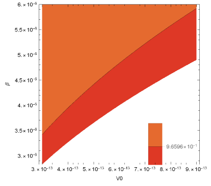
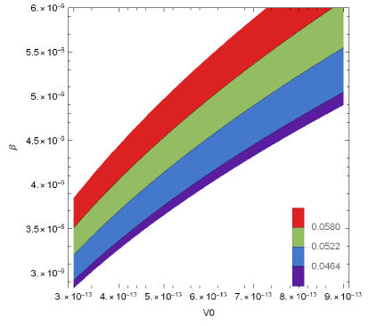
Figure 1: Contour plots of the spectral index of primordial curvature perturbations (left plot) and tensor-to-scalar ratio (right plot) at the first horizon crossing that correspond to values $n_{\mathcal{S}}=[0.9607,0.9691]$ and $r<0.064$ respectively and also satisfy the approximation (14), for $N=60$.

The second slow-roll index also takes a simple form, $\epsilon_{2}=\frac{4\mathcal{V}_{0}}{3\kappa^{4}M^{2}\varphi^{2}}$, while $\epsilon_{3}=\frac{4\mathcal{V}_{0}\left(3\kappa^{2}M^{2}+2\mathcal{V}_{0}\right)}{-27\kappa^{4}M^{4}-6\kappa^{2}M^{2}\mathcal{V}_{0}\left(\kappa^{2}\varphi^{2}-1\right)+4\mathcal{V}_{0}^{2}}$, and $\epsilon_{4}$ is more complicated so we do not quote here. Also, the value of the scalar field at the first horizon crossing, namely $\varphi_{i}$, can easily be found using Eq. (35) that gives the $e$-foldings number along with the $\varphi_{f}$ we obtained earlier, so upon solving (35) after performing the integration, we get $\varphi_{i}=\frac{\sqrt{\frac{2}{3}}\sqrt{2\mathcal{V}_{0}+3M^{2}\kappa^{2}+6M^{2}N\kappa^{2}}}{M\kappa^{2}}.$

We can now calculate the slow-roll indices, the spectral index, the tensor-to-scalar ratio, the tensor spectral index and the amplitude of the scalar curvature perturbations at the first horizon crossing by setting $\varphi=\varphi_{i}$. The final relations are omitted for brevity. We generally assume that $M=\beta/\kappa$, where $\beta$ is some dimensionless parameter, therefore the model has three dimensionless free parameters: $\beta$, $\mathcal{V}_{0}$ and the $e$-foldings number, $N$, hence it is a three parameter model. What we generally expect is that $\mathcal{V}_{0}$ will be differently constrained in the $\mathcal{R}^{2}$-corrected theory than it is constrained in the simple quadratic inflation model. We shall examine for which values of these parameters this model provides a viable inflationary phenomenology. According to the latest Planck data, the spectral index and the tensor-to-scalar ratio are constrained as following Planck:2018jri ,

$$n_{\mathcal{S}}=0.9649\pm 0.0042\ ,\ r<0.064.$$ (41)

Furthermore, the power spectrum of the scalar perturbations should be constrained to the values,

$$\mathcal{P}_{\zeta}(k)=2.19\pm 0.02\times 10^{-9},$$ (42)

for a viable theory. As it occurs, the amplitude of the scalar perturbations basically constrains severely the final model, and our analysis of the parameter space showed that it is compatible with the Planck constraints Planck:2018jri when the values for the free parameters are of order $\mathcal{V}_{0}\sim\mathcal{O}(10^{-13})$ and $\beta\sim\mathcal{O}(10^{-6})$. For example, if we set $\mathcal{V}_{0}=9.37\times 10^{-13}$, $\beta=6.8\times 10^{-6}$ for $N=60$ we get,

$$n_{\mathcal{S}}=0.96611,\,\,\,r=0.063968,\,\,\,n_{\mathcal{T}}=-0.00799592\,,$$ (43)

so the phenomenology is compatible with the latest Planck data Planck:2018jri and the tensor spectrum is red-tilted. As for the amplitude of the scalar perturbations, we have,

$$\mathcal{P}_{\zeta}(k)=2.19216\times 10^{-9},$$ (44)

so this quantity too is compatible with the Planck constraints. We remind that we should constantly check the validity of the approximations (13), (14) for the values of the free parameters that we select. The model is proven to be compatible with the latest Planck constraints, for a wide range of the free parameters $\mathcal{V}_{0}$ and $\beta$.

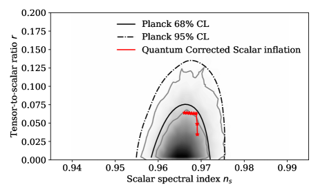
Figure 2: Confrontation of the $\mathcal{R}^{2}$ corrected quadratic inflation gravity model (red curve) with the 2018 Planck constraints for $N$ varying in the range $N=[60,67]$ and a selection of values for the free parameters that result in values of the observational indices in accordance with the latest Planck constraints, respecting the approximations following the theory.

Indeed, the values used in our example are not the only values that can make the observational indices simultaneously compatible with the Planck constraints, as can be seen in Fig.1, where we present the contour plots of the spectral index and the tensor-to-scalar ratio for a range of values of the free parameters,that correspond $n_{\mathcal{S}}=[0.9607,0.9691]$ and $r<0.064$ and also obey the approximations (13) and (14), that hold a key role in our analysis. Moreover, in Fig.2 we also present the 2018 Planck likelihood curves and one can notice that the $\mathcal{R}^{2}$-corrected quadratic inflation theory is well fitted within those likelihood curves. The resulting line is composed by a variety of points for different values of the free parameters, $\mathcal{V}_{0},\beta$ and for number of $e$-foldings in the range $N=[60,67]$ such, that the values of the observational indices calculated satisfy the Planck constraints (41), the amplitude of the scalar perturbations falls within the range of (42) and the approximations (13),(14) hold true. Generally, the approximation (13) holds true for a very wide range of values of $\mathcal{V}_{0}$ and $\beta$, however we cannot say the same for (14). The latter approximation is harder to satisfy, thus it impacts the allowed values of the free parameters resulting in further limitations to the values of $n_{\mathcal{S}}$ and $r$. The reason that we stopped adding points at $N=67$ is that for greater values of $N$ there are no values of $\mathcal{V}_{0}$ and $\beta$ that result in the spectral index taking values within $n_{\mathcal{S}}=[0.9607,0.9691]$ and in simultaneous validity of the approximation (14) along with the amplitude of the scalar perturbations satisfying (42). This behavior is depicted in Fig. 3, where the upper contours of the plot represent the values of $\frac{\kappa^{2}\dot{\varphi}^{2}}{M^{2}}$, the lower contours the values of $n_{\mathcal{S}}$ that satisfy the Planck constraints and the thin textured line the accepted values for the amplitude of the scalar perturbations. It is obvious that there is no overlapping of these plots for any values of the free parameters, a characteristic that becomes more intense as $N$ increases beyond $N>67$.

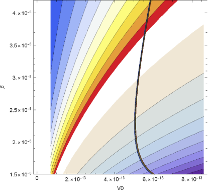
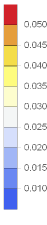
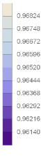
Figure 3: Contour plot of the spectral index of primordial curvature perturbations (lower contours), the factor $\frac{\kappa^{2}\dot{\varphi}^{2}}{M^{2}}$ (upper contours) and the amplitude of the scalar curvature perturbations (dark line) at the first horizon crossing, for $N=68$, indicating that a simultaneous satisfaction of their constraints cannot be achieved for any values of the free parameters when $N>67$.

Summarizing, the $\mathcal{R}^{2}$ quantum corrected quadratic inflation model yields an inflationary phenomenology which is compatible with the latest Planck constraints, in contrast to the simple quadratic inflation model, which is incompatible with the Planck data. In principle more examples of this sort can be studied, but the analysis is more or less the same, so we do not go in details on extra models.

IV Conclusions

In this work we studied a generalized $f(\mathcal{R},\varphi)$ gravity framework, in which a canonical scalar field theory is considered in the presence of string theory originating higher order curvature quantum correction terms. We considered for simplicity an $\mathcal{R}^{2}$ term and we investigated in detail the effect of the $\mathcal{R}^{2}$ correction term on the equations of motion of scalar field theory at leading order. After deriving the field equations of the combined $\mathcal{R}^{2}$-corrected scalar field theory, we presented the final form of the slow-roll indices for this theory. As we showed, the latter acquire quite elegant final forms, in which the leading order effect of the $\mathcal{R}^{2}$ quantum corrections is directly seen in each one of them. The resulting theoretical framework was tested with respect to its inflationary aspects. For a test model we chose the quadratic inflation model, which is a non-viable single scalar field model when it is considered by itself. As we showed, the $\mathcal{R}^{2}$-corrected quadratic inflation model yields a viable inflationary phenomenology. With regard to the inflationary phenomenology, we mainly focused on the spectral index of the primordial scalar curvature perturbations, the tensor-to-scalar ratio, the tensor spectral index and the amplitude of the scalar perturbations. One notable feature is the fact that the multiplicative parameter of the potential, which we denoted as $\mathcal{V}_{0}$, is constrained differently in comparison to the simple quadratic inflation model. Indeed, the final form of the amplitude of the scalar perturbations in the $\mathcal{R}^{2}$-corrected quadratic inflation theory is different from that of the simple quadratic inflation theory, thus $\mathcal{V}_{0}$ can take different values compared to the simple quadratic inflation case. The next step toward the research line we adopted in this paper, is to considered combinations of quantum corrections in the simple scalar field theory. The case of an $\mathcal{R}^{2}$-corrected Einstein-Gauss-Bonnet theory was considered in Ref. Odintsov:2020ilr , and it was shown that a viable phenomenology can be obtained for these models, for both minimal and non-minimally coupled scalar field models. What has not been studied yet in the literature is considering $\mathcal{R}^{3}$ corrections, which basically originate from order-six higher curvature derivatives in the quantum corrected scalar field action (2). We will address this issue in the near future.

Finally, let us comment that the whole point of this work was to simply introduce an alternative to the standard scalar field inflation including $R^{2}$ corrections in the scalar field Lagrangian. The potential we chose for checking our formalism is an $\phi^{2}$ potential, which without the $R^{2}$ term is not compatible with the Planck data. But with our formalism we showed that the model is viable, if $R^{2}$ corrections are considered. So our intention was not to compare our model with the standard $R^{2}$ model, but to see what happens if one uses both scalar fields and higher order curvature terms in the inflationary Lagrangian. If those are considered together in the Jordan frame, we showed how such a framework can lead to sensible results. In Einstein frame descriptions this is not possible though because dealing analytically with two scalar fields is impossible to work easily.

References

- (1) A. D. Linde, Lect. Notes Phys. 738 (2008) 1 [arXiv:0705.0164 [hep-th]].
- (2) D. S. Gorbunov and V. A. Rubakov, “Introduction to the theory of the early universe: Cosmological perturbations and inflationary theory,” Hackensack, USA: World Scientific (2011) 489 p;
- (3) A. Linde, arXiv:1402.0526 [hep-th];
- (4) D. H. Lyth and A. Riotto, Phys. Rept. 314 (1999) 1 [hep-ph/9807278].
- (5) K. N. Abazajian et al. [CMB-S4], [arXiv:1610.02743 [astro-ph.CO]].
- (6) M. H. Abitbol et al. [Simons Observatory], Bull. Am. Astron. Soc. 51 (2019), 147 [arXiv:1907.08284 [astro-ph.IM]].
- (7) M. Kamionkowski and E. D. Kovetz, Ann. Rev. Astron. Astrophys. 54 (2016) 227 doi:10.1146/annurev-astro-081915-023433 [arXiv:1510.06042 [astro-ph.CO]].
- (8) S. Hild, M. Abernathy, F. Acernese, P. Amaro-Seoane, N. Andersson, K. Arun, F. Barone, B. Barr, M. Barsuglia and M. Beker, et al. Class. Quant. Grav. 28 (2011), 094013 doi:10.1088/0264-9381/28/9/094013 [arXiv:1012.0908 [gr-qc]].
- (9) J. Baker, J. Bellovary, P. L. Bender, E. Berti, R. Caldwell, J. Camp, J. W. Conklin, N. Cornish, C. Cutler and R. DeRosa, et al. [arXiv:1907.06482 [astro-ph.IM]].
- (10) T. L. Smith and R. Caldwell, Phys. Rev. D 100 (2019) no.10, 104055 doi:10.1103/PhysRevD.100.104055 [arXiv:1908.00546 [astro-ph.CO]].
- (11) J. Crowder and N. J. Cornish, Phys. Rev. D 72 (2005), 083005 doi:10.1103/PhysRevD.72.083005 [arXiv:gr-qc/0506015 [gr-qc]].
- (12) T. L. Smith and R. Caldwell, Phys. Rev. D 95 (2017) no.4, 044036 doi:10.1103/PhysRevD.95.044036 [arXiv:1609.05901 [gr-qc]].
- (13) N. Seto, S. Kawamura and T. Nakamura, Phys. Rev. Lett. 87 (2001), 221103 doi:10.1103/PhysRevLett.87.221103 [arXiv:astro-ph/0108011 [astro-ph]].
- (14) S. Kawamura, M. Ando, N. Seto, S. Sato, M. Musha, I. Kawano, J. Yokoyama, T. Tanaka, K. Ioka and T. Akutsu, et al. [arXiv:2006.13545 [gr-qc]].
- (15) A. Weltman, P. Bull, S. Camera, K. Kelley, H. Padmanabhan, J. Pritchard, A. Raccanelli, S. Riemer-Sørensen, L. Shao and S. Andrianomena, et al. Publ. Astron. Soc. Austral. 37 (2020), e002 doi:10.1017/pasa.2019.42 [arXiv:1810.02680 [astro-ph.CO]].
- (16) A. Codello and R. K. Jain, Class. Quant. Grav. 33 (2016) no.22, 225006 doi:10.1088/0264-9381/33/22/225006 [arXiv:1507.06308 [gr-qc]].
- (17) S. Nojiri, S. D. Odintsov and V. K. Oikonomou, Phys. Rept. 692 (2017) 1 [arXiv:1705.11098 [gr-qc]].
-
(18)
S. Capozziello, M. De Laurentis,
Phys. Rept. 509, 167 (2011);
V. Faraoni and S. Capozziello, Fundam. Theor. Phys. 170 (2010). - (19) S. Nojiri, S.D. Odintsov, eConf C0602061, 06 (2006) [Int. J. Geom. Meth. Mod. Phys. 4, 115 (2007)].
- (20) S. Nojiri, S.D. Odintsov, Phys. Rept. 505, 59 (2011);
- (21) A. de la Cruz-Dombriz and D. Saez-Gomez, Entropy 14 (2012) 1717 [arXiv:1207.2663 [gr-qc]].
- (22) G. J. Olmo, Int. J. Mod. Phys. D 20 (2011) 413 [arXiv:1101.3864 [gr-qc]].
- (23) Y. Ema, Phys. Lett. B 770 (2017), 403-411 doi:10.1016/j.physletb.2017.04.060 [arXiv:1701.07665 [hep-ph]].
- (24) Y. Ema, K. Mukaida and J. Van De Vis, JHEP 02 (2021), 109 doi:10.1007/JHEP02(2021)109 [arXiv:2008.01096 [hep-ph]].
- (25) V. R. Ivanov and S. Y. Vernov, [arXiv:2108.10276 [gr-qc]].
- (26) S. Gottlober, J. P. Mucket and A. A. Starobinsky, Astrophys. J. 434 (1994), 417-423 doi:10.1086/174743 [arXiv:astro-ph/9309049 [astro-ph]].
- (27) A. de la Cruz-Dombriz, E. Elizalde, S. D. Odintsov and D. Sáez-Gómez, JCAP 05 (2016), 060 doi:10.1088/1475-7516/2016/05/060 [arXiv:1603.05537 [gr-qc]].
- (28) V. M. Enckell, K. Enqvist, S. Rasanen and L. P. Wahlman, JCAP 01 (2020), 041 doi:10.1088/1475-7516/2020/01/041 [arXiv:1812.08754 [astro-ph.CO]].
- (29) A. Karam, T. Pappas and K. Tamvakis, JCAP 02 (2019), 006 doi:10.1088/1475-7516/2019/02/006 [arXiv:1810.12884 [gr-qc]].
- (30) J. Kubo, J. Kuntz, M. Lindner, J. Rezacek, P. Saake and A. Trautner, JHEP 08 (2021), 016 doi:10.1007/JHEP08(2021)016 [arXiv:2012.09706 [hep-ph]].
- (31) D. Gorbunov and A. Tokareva, Phys. Lett. B 788 (2019), 37-41 doi:10.1016/j.physletb.2018.11.015 [arXiv:1807.02392 [hep-ph]].
- (32) X. Calmet and I. Kuntz, Eur. Phys. J. C 76 (2016) no.5, 289 doi:10.1140/epjc/s10052-016-4136-3 [arXiv:1605.02236 [hep-th]].
- (33) V. K. Oikonomou, Annals Phys. 432 (2021), 168576 doi:10.1016/j.aop.2021.168576 [arXiv:2108.04050 [gr-qc]].
- (34) S. D. Odintsov, V. K. Oikonomou and F. P. Fronimos, [arXiv:2108.11231 [gr-qc]].
- (35) S. D. Odintsov, V. K. Oikonomou and L. Sebastiani, Nucl. Phys. B 923 (2017), 608-632 doi:10.1016/j.nuclphysb.2017.08.018 [arXiv:1708.08346 [gr-qc]].
- (36) A. A. Starobinsky, Phys. Lett. B 91 (1980), 99-102 doi:10.1016/0370-2693(80)90670-X
- (37) F. L. Bezrukov and M. Shaposhnikov, Phys. Lett. B 659 (2008), 703-706 doi:10.1016/j.physletb.2007.11.072 [arXiv:0710.3755 [hep-th]].
- (38) S. A. Appleby, R. A. Battye and A. A. Starobinsky, JCAP 06 (2010), 005 doi:10.1088/1475-7516/2010/06/005 [arXiv:0909.1737 [astro-ph.CO]].
- (39) J. c. Hwang and H. Noh, Phys. Rev. D 71 (2005) 063536 doi:10.1103/PhysRevD.71.063536 [gr-qc/0412126].
- (40) Y. Akrami et al. [Planck], Astron. Astrophys. 641 (2020), A10 doi:10.1051/0004-6361/201833887 [arXiv:1807.06211 [astro-ph.CO]].
- (41) S. D. Odintsov, V. K. Oikonomou and F. P. Fronimos, Annals Phys. 424 (2021), 168359 doi:10.1016/j.aop.2020.168359 [arXiv:2011.08680 [gr-qc]].