Imaging Conductivity from Current Density Magnitude using Neural Networks

Abstract

Conductivity imaging represents one of the most important tasks in medical imaging. In this work we develop a neural network based reconstruction technique for imaging the conductivity from the magnitude of the internal current density. It is achieved by formulating the problem as a relaxed weighted least-gradient problem, and then approximating its minimizer by standard fully connected feedforward neural networks. We derive bounds on two components of the generalization error, i.e., approximation error and statistical error, explicitly in terms of properties of the neural networks (e.g., depth, total number of parameters, and the bound of the network parameters). We illustrate the performance and distinct features of the approach on several numerical experiments. Numerically, it is observed that the approach enjoys remarkable robustness with respect to the presence of data noise.
Key words: conductivity imaging, current density imaging, neural network, generalization error

1 Introduction

The conductivity value varies widely with soft tissue types [24, 52] and its accurate imaging can provide valuable information about the physiological and pathological conditions of tissue. This underpins several important medical imaging modalities [13, 2, 70]. For example, electrical impedance tomography (EIT) [13] aims at recovering the interior conductivity distribution from given pairs of flux / voltage on the object’s boundary. However, it is severely ill-posed, which makes it very challenging to develop a stable numerical algorithm to accurately reconstruct the conductivity [13]. Especially, the attainable resolution of the reconstruction is fairly limited. To lessen the inherent degree of ill-posedness, researchers have proposed several novel conductivity imaging modalities, e.g., magnetic resonance electrical impedance tomography (MREIT) / current density impedance imaging (CDII), impedance-acoustic tomography, acousto-electric tomography and magneto-acoustic tomography with magnetic induction. All these imaging modalities employ internal data that are derived from other modalities (hence the term coupled-physics imaging). See the reviews [70] and [5] for extensive discussions on the mathematical model and the mathematical theory, respectively. The availability of internal data promises reconstructions with much improved resolution.

In this work we focus on current density impedance imaging (CDII) [53]. Let $\Omega\subset\mathbb{R}^{d}$, $d=2,3$, be an open bounded Lipschitz domain modeling the conducting body with a boundary $\partial\Omega$. The relation between the voltage $u$ and the conductivity $\sigma$ is described by

$$\left\{\begin{split}-\nabla\cdot(\sigma\nabla u)&=0,\quad\mbox{in }\Omega,\\ u&=g,\quad\mbox{on }\partial\Omega,\end{split}\right.$$ (1.1)

where $g$ is the applied boundary voltage. In CDII, the current density $J$ is given by $J(x)=-\sigma\nabla u(x)$, for $x\in\Omega$. In practice, one employs an MRI scanner to capture the internal magnetic flux density data $\vec{b}$ induced by an externally injected current [36, 61, 31, 25] and then obtains the current density $J$ according to Ampere’s law $J=\mu_{0}^{-1}\nabla\times\vec{b}$, where $\mu_{0}$ is the magnetic permeability. This requires measuring all components of the magnetic flux $\vec{b}$, which may be challenging in practice, as it requires a rotation of the object being imaged or of the MRI scanner. CDII aims at recovering the conductivity $\sigma$ from $a(x)\equiv|J(x)|$ in $\Omega$, the magnitude of one current density field.

CDII has been intensively studied in the past decade, and a number of important theoretical results have been obtained. Nachman et al [53] established the uniqueness of the recovery from one internal measurement $a$ together with Cauchy data on a part of the object’s boundary. Later, the uniqueness was shown also for anisotropic conductivity with a known conformal class [28]. The Hölder conditional stability for the nonlinear inverse problem of recovering the conductivity distribution $\sigma$ from one internal measurement was proved in [48]. The case of partial data (i.e., a partial knowledge of one current density field generated inside a body) has also been proved [49]. The conditional stability of the inverse problem under fairly general assumptions was shown in [42].

The development of novel reconstruction algorithms has also received much attention. One popular algorithm is an iterative method to solve the weighted least-gradient formulation [54], which iteratively solves a well-posed direct problem, and the authors proved that the sequence of iterates converges; See Section 2.1 for more details about the derivation. It has been extended to other scenarios, e.g., complete electrode model [55]. An alternative approach is based on the level set [53, 67]. A linearized reconstruction technique was developed recently in [73]. The more conventional output least-squares formulation has not been employed for CDII reconstruction, but it applies more or less directly (see [1, 41] for conductivity imaging from related internal data, and [29] for iterative reconstruction).

In this work, we develop a new numerical method for the recovery of the conductivity $\sigma$ from the current density magnitude $a(x)$. It is based on the weighted least-gradient reformulation of the inverse problem, which has inspired the iterative algorithm in [54]. Instead of solving the variational problem iteratively, we solve a relaxed version of the problem directly using neural networks. The approach is flexible with domain geometry and problem data, and capitalizes directly on recent algorithmic innovations in machine learning, e.g., stochastic optimization [14] and automatic differentiation [11]. The numerical results in Section 4 clearly demonstrate the significant potential of the approach: it enjoys remarkable robustness with respect to the presence of a large amount of data noise. Further, we provide a preliminary analysis of the neural network approximation to the relaxed least-gradient problem, in terms of the approximation and statistical errors. The main tools in the analysis include approximation theory of neural networks [26] and Rademacher complexity from statistical learning theory [63]. The analysis sheds light into the choice of several important algorithmic parameters, e.g., network width and depth, and the number of sampling points in the domain and on the boundary.

In recent years, the use of deep neural networks (DNNs) for solving PDEs has received much attention, and several different methods have been developed; see the review [21] for a recent overview on various ways of using neural networks for different classes of PDEs and a fairly extensive list of relevant references. One notable idea is to utilize neural networks to approximate solutions of PDEs directly, which can be traced back to the 1990s [18, 40]. Notable recent developments include physics-informed neural networks [58], deep Galerkin method [64] and deep Ritz method [22] etc. The first two methods are based on least-squares type residual minimization for solving PDEs. The deep Ritz method is based on the Ritz variational formulation of the elliptic problem. This work adopts a deep Ritz method to the weighted least-gradient problem arising in CDII. Despite the great empirical successes of these methods, rigorous numerical analysis of neural network based PDE solvers remains very challenging and is still in its infancy [44, 19, 71, 43, 35, 34, 30]. The important works [44, 71, 43, 30] derived a priori error bounds on the approximations obtained by two-layer neural networks under suitable regularity conditions on the solutions, whereas the work [34] studied DNNs for standard second-order elliptic PDEs with Robin boundary conditions. The present work extends the analysis in [34] to the weighted least-gradient problem arising in CDII.

Very recently, the use of DNNs for solving PDE inverse problems also started to receive attention, and existing methods can roughly be divided into two groups: supervised [62, 37, 27] and unsupervised [6, 7, 57, 72]. The methods in the former group rely on the availability of paired training data, and are essentially concerned with learning the forward operators or its (regularized) inverses, and the methods in the latter group exploit essentially the extraordinary expressivity as universal function approximators. Khoo and Ying [37] proposed a novel neural network architecture, SwitchNet, for solving the wave equation based inverse scattering problems via constructing maps between the scatterers and the scattered field using training data. Seo et al. [62] developed a supervised approach for the solution of nonlinear inverse problems using a low dimensional manifold for the solution approximation, converting it into a well-posed one using variational autoencoder, and demonstrated the idea on time difference EIT. Guo and Jiang [27] developed a neural network analogue for the direct sampling method for EIT. The works [6] and [7] investigated image reconstruction in the classical EIT problem, using the weak formulation and the least-squares formulation (but also with the $L^{\infty}$ norm consistency), respectively. Pakravan et al [57] developed a hybrid approach, aiming at blending high expressivity of DNNs with the accuracy and reliability of traditional numerical methods for PDEs, and showed the approach for recovering the variable diffusion coefficient in one- and two-dimensional elliptic PDEs. All these works have presented very encouraging empirical results for a range of PDE inverse problems, and clearly demonstrated the significant potentials of DNNs in solving PDE inverse problems. The approach proposed in this work belongs to the second group, but unlike the existing approaches, it does not directly approximate the unknown conductivity $\sigma$ and thus differs substantially from existing approaches.

The rest of the paper is organized as follows. In Section 2 we develop a neural network based approach for imaging the conductivity. Then in Section 3 we provide an analysis of the neural network based approach, and derive a convergence rate for the neural network approximation in terms of properties of the neural network, e.g., the activation function, depth, number of parameters, and parameter bound. In Section 4, we present extensive numerical experiments to show its performance and the impact of various algorithmic parameters on the reconstruction error (number of training points, network parameters and noise levels), and also present a comparative study of the approach with an existing iterative reconstruction approach [54].

2 Reconstruction algorithm

In this section, we describe the proposed imaging algorithm. It is essentially a neural network discretization of a relaxation of the variational formulation proposed by Nachman et al [54]. A preliminary analysis of the neural network approximation is given in Section 3.

2.1 Variational formulation

First we briefly recall a variational formulation from [54]. By representing $\sigma=\frac{a}{|\nabla u|}$ in accordance with Ohm’s law, problem (1.1) can be recast into the following Dirichlet problem for the weighted 1-Laplacian

$$\left\{\begin{aligned} \nabla\cdot\Big{(}a\frac{\nabla u}{|\nabla u|}\Big{)}&=0,\quad\mbox{in }\Omega,\\ u&=g,\quad\mbox{on }\partial\Omega.\end{aligned}\right.$$ (2.1)

This was originally proposed by Kim et al [38], who also showed nonuniqueness of the solution when the problem is equipped with a Neumann boundary condition. Formulation (2.1) was utilized by work [53] for recovering the conductivity $\sigma$ from Cauchy data on a part of the boundary (along with the interior data) on a two-dimensional domain. Due to the singularity and elliptic degeneracy of the differential operator, the concept of a solution requires some care. Therefore, as a mathematical model of CDII, Nachman et al [54] employed the following weighted least gradient (Dirichlet) problem

$$\min_{u\in W^{1,1}(\Omega)\cap C(\overline{\Omega}),Tu=g}\Big{\{}\mathcal{J}(u)=\int_{\Omega}a|\nabla u|\mathrm{d}x\Big{\}},$$ (2.2)

where $T$ is the trace operator, i.e., $Tu=u\lvert_{\partial\Omega}$. The equivalence can be seen by computing the Euler–Lagrange equation of the functional $\mathcal{J}$ and observing that it formally satisfies problem (2.1). It was proved in [54, Theorem 1.3] that if $g\in C^{1,\nu}(\partial\Omega)$, $a\in C^{\nu}(\overline{\Omega})$, $\nu\in(0,1)$, and $a>0$ a.e. in $\Omega$, and the data $(g,a)$ are admissible (i.e., there exists a conductivity $\sigma$ that is essentially bounded and bounded away from zero such that if $u\in H^{1}(\Omega)$ is a weak solution to problem (1.1) then $a=\sigma|\nabla u|$), then problem (2.2) is uniquely solvable in $W^{1,1}(\Omega)\cap C(\overline{\Omega})$ and $\sigma=\frac{a}{|\nabla u|}$ is Hölder continuous. It was also shown that problem (2.1) is, formally, the Euler-Lagrange equation of the functional $\mathcal{J}(u)$ in (2.2), and that the solution of (2.2) is a weak solution to (2.1).

From the point of view of calculus of variation, the space $W^{1,1}(\Omega)$ is not the most convenient choice for studying problem (2.2) [56]. Indeed, the minimizing sequences stay bounded in $W^{1,1}(\Omega)$. However, due to its non-reflexivity, $\mathcal{J}$ is no longer weakly lower semicontinuous in $W^{1,1}(\Omega)$ (since $L^{1}_{loc}(\Omega)$ limits of functions in $W^{1,1}(\Omega)$ may no longer belong to $W^{1,1}(\Omega)$). Thus, it is natural to extend $\mathcal{J}(u)$ in (2.2) to the space $BV(\Omega)$ of functions of bounded variation, which preserves the lower-semicontinuity. These considerations naturally lead to the study of the following weighted least-gradient problems in the space $BV(\Omega)$ [56]

$$\min_{u\in BV(\Omega),Tu=g}\Big{\{}\mathcal{J}(u)=\int_{\Omega}a(x)|Du|\Big{\}},$$ (2.3)

where the distributional derivative $Du$ is a signed Radon measure that can be decomposed into its absolutely continuous and singular parts as $Du=D^{a}u+D^{s}u$, with $D^{a}u=\nabla u\mathcal{L}^{d}$, where $\nabla u$ is the Radon-Nikodym derivative of the measure $Du$ with respect to the Lebesgure measure $\mathcal{L}^{d}$, and $D^{s}u$ denotes the singular part. The existence and uniqueness results of problem (2.3) were established for either the case $a\in C^{1,1}(\overline{\Omega})$, $g\in C(\partial\Omega)$ [33] or the case $a\in C(\overline{\Omega})$, $a\geq 0$, and that the pair $(g,a)$ is admissible [50].

Once a minimizer $u$ to problem (2.3) is found, the conductivity $\sigma$ can be recovered by $\sigma=\frac{a}{|\nabla u|}$, following the definition of the current density magnitude $a$. These observations and the convexity of the energy functional $\mathcal{J}$ motivated several algorithms for recovering the conductivity $\sigma$ [54, 51]. Nachman et al [54] developed an iterative procedure for minimizing problem (2.2) and then recovering the conductivity $\sigma$. Specifically, given an initial guess $\sigma^{0}$, they proposed to repeat the following two steps alternatingly

• Solve for $u^{n}$ from the second-order elliptic PDE

  $$\left\{\begin{split}-\nabla\cdot(\sigma^{n}\nabla u^{n})&=0,\quad\mbox{in }\Omega,\\ u^{n}&=g,\quad\mbox{on }\partial\Omega.\end{split}\right.$$

• Update the conductivity $\sigma$ by $\sigma^{n+1}=\frac{a}{|\nabla u^{n}|}$.

The authors proved the convergence of the sequence $\{u^{n}\}_{n=1}^{\infty}$ to the minimizer of functional $\mathcal{J}$ in $H^{1}(\Omega)$ for admissible pairs $(g,a)$ [54, Proposition 4.4]. This algorithm is appealing since it is easy to implement, and converges within tens of iteration. The main cost is to solve one elliptic PDE at each iteration. It will be employed as the baseline algorithm in the numerical experiments. Note that the algorithm does not incorporate regularization explicitly [32]. Due to the ill-poseness, in the presence of data noise, early stopping is needed in order to obtain satisfactory reconstructions. However, the issue of early stopping has not been studied so far for the algorithm.

2.2 Proposed algorithm

In this work, we take a slightly different route. Instead of iterative update, we propose to solve the minimization problem (2.3) directly by using neural networks to approximate the minimizer $u$ (with parameter $\theta$), and then to recover the conductivity $\sigma$ using the defining relation $\sigma=\frac{a}{|\nabla u|}$ from Ohm’s law. More specifically, we proceed in the following two steps:

• Find a neural network approximation $u_{\theta}$ to problem (2.3) by minimizing a suitable loss.

• Recover the conductivity $\sigma$ by $\sigma=\frac{a}{|\nabla u_{\theta}|}$.

The crucial step to realize the algorithm numerically is to solve (2.3) stably. This is nontrivial due to nonsmoothness of the functional $\mathcal{J}$. Further, the imposition of the essential boundary condition $Tu=g$ is nontrivial, due to the nonlocality of neural networks. For special geometries, one may construct neural networks that satisfy the boundary condition exactly, but generally this is challenging. Thus, we employ an alternative formulation of problem (2.3) from [45] (see also [47, 16]), using the concept of the space of total variation with respect to an anisotropy defined below. Throughout we make the following assumption on the data $a$, which is also known as the continuity and coercivity of the metric integrand.

Assumption 2.1.

$a\in C(\overline{\Omega})$, and there exist constants $\alpha_{0},\alpha_{1}>0$ with $\alpha_{1}>\alpha_{0}$ such that $\alpha_{0}\leq a\leq\alpha_{1}$ in $\Omega$.

Now we recall the space $BV_{a}(\Omega)$ [47, 16]. Clearly when $a(x)\equiv 1$ in $\Omega$, it recovers the standard space $BV(\Omega)$ of functions of bounded variation.

Definition 2.1.

Let $u\in L^{1}(\Omega)$. Then the $a$-total variation of $u$ in $\Omega$ is defined as

$$\int_{\Omega}|Du|_{a}:=\sup_{\varphi\in K_{a}(\Omega)}\int_{\Omega}u\nabla\cdot\varphi,\quad\mbox{with }K_{a}(\Omega)=\{\varphi\in C_{0}^{1}(\Omega;\mathbb{R}^{d}):|\varphi(x)|\leq a(x)\mbox{ in }\Omega\},$$

and let

$$BV_{a}(\Omega)=\{u\in L^{1}(\Omega):\int_{\Omega}|Du|_{a}<\infty\},$$

which is a Banach space when endowed with the norm

$$\|u\|_{BV_{a}(\Omega)}=\|u\|_{L^{1}(\Omega)}+\int_{\Omega}|Du|_{a}.$$

Note that under Assumption 2.1, there hold $BV_{a}(\Omega)=BV(\Omega)$ in the sense of set (but endowed with different norms), and further

$$\alpha_{0}\int_{\Omega}|Du|\leq\int_{\Omega}|Du|_{a}\leq\alpha_{1}\int_{\Omega}|Du|.$$

Given a function $g\in L^{1}(\partial\Omega)$, problem (2.2) can be equivalently written as

$$\min\mathcal{J}_{g}(u)=\left\{\begin{aligned} \int_{\Omega}a|\nabla u|\mathrm{d}x,&\quad\mbox{if }u\in W^{1,1}(\Omega),Tu=g,\\ +\infty,&\quad\mbox{otherwise}.\end{aligned}\right.$$

In [47, Theorem 4] (see also [16, Theorem 3.6] and [45, Proposition 3.1]), it was proved that the functional $\mathcal{J}_{g}$ admits the following relaxation to $L^{\frac{d}{d-1}}(\Omega)$

$$\mathcal{L}(u)=\left\{\begin{aligned} \int_{\Omega}|Du|_{a}+\int_{\partial\Omega}a|Tu-g|\mathrm{d}s,&\quad u\in BV_{a}(\Omega),\\ +\infty,&\quad u\in L^{\frac{d}{d-1}}(\Omega)\setminus BV_{a}(\Omega),\end{aligned}\right.$$ (2.4)

in the following sense

$$\mathcal{L}(u)=\inf\Big{\{}\liminf_{n\to\infty}\mathcal{J}_{g}(u_{n}):u_{n}\to u\mbox{ in }L^{1}(\Omega),\ u_{n}\in W^{1,1}(\Omega),Tu_{n}=g\Big{\}}.$$

Therefore, for every $u\in BV_{a}(\Omega)$, there exists a sequence $\{u_{n}\}_{n=1}^{\infty}\subset W^{1,1}(\Omega)$ with $Tu_{n}=g$ such that $u_{n}\to u$ in $L^{1}(\Omega)$ and

$$\int_{\Omega}a(x)|\nabla u_{n}(x)|\mathrm{d}x\to\mathcal{L}(u).$$

In particular, this implies the functional $\mathcal{L}$ is weakly lower semicontinuous, which automatically guarantees the existence of a minimizer.

The relaxed functional $\mathcal{L}$ is convex and weakly lower semicontinuous in $L^{\frac{d}{d-1}}(\Omega)$. Furthermore, we have the following results which connect the relaxed functional (2.4) to problem (2.3) (see [45, Definition 3.4] for the precise definition of a solution $u$ to problem (2.1)). Thus, under certain conditions, the solution of (2.4) coincides with that of (2.3).

Theorem 2.1.

Under Assumption 2.1, for each $g\in L^{1}(\Omega)$, there exists a solution $u$ to problem (2.1). Further, for $u\in BV_{a}(\Omega)$ satisfying $Tu=g$, the following three statements are equivalent.

• $u$ is a solution of problem (2.1).

• $u$ is a function of the weighted least gradient in $\Omega$, i.e., solves problem (2.3).

• $\mathcal{L}(u)\leq\mathcal{L}(v)$ for all $v\in BV_{a}(\Omega)$.

Proof.

Note that Assumption 2.1 implies that the metric integrand $\phi(x,\xi)=a(x)|\xi|$ is continuous and coercive in $\Omega$. The first statement can be found in [45, Theorem 3.6], and the equivalence statements are taken from [45, Corllary 3.9], ∎

In practice, it is beneficial to introduce a weighing parameter $\gamma>1$ to the boundary integral

$$\mathcal{L}_{\gamma}(u)=\int_{\Omega}a|Du|+\gamma\int_{\partial\Omega}a|Tu-g|\mathrm{d}s.$$ (2.5)

Formally, it can be viewed as a nonstandard penalized formulation to impose the boundary condition only weakly, and this idea is widely used in the context of finite element methods [4]. However, the existence of a minimizer $u^{*}$ in $BV(\Omega)$ is generally unclear, since the trace operator in $BV(\Omega)$ is not continuous with respect to the weak star convergence in $BV(\Omega)$. The existence will be assumed for the analysis below in Section 3.

Remark 2.1.

There are alternative penalized formulations that ensure the existence of a minimizer:

$$\mathcal{L}_{\gamma,\epsilon}(u)=\int_{\Omega}a|\nabla u(x)|\ \mathrm{d}x+\frac{\gamma}{2}\int_{\partial\Omega}|Tu-g|^{2}\ \mathrm{d}s+\frac{\epsilon}{2}\int_{\Omega}|\nabla u|^{2}\mathrm{d}x,$$

with small $\epsilon>0$. This formulation was studied in [66]. The neural network approach described below can be extended directly and the analysis also holds upon minor changes.

2.3 Discretization via neural networks

Now we describe the discretization of problem (2.5) via neural networks. We employ the standard fully connected feedforward neural networks, in which each neuron is connected to neurons in the successive layer by an affine-linear map, and then followed by a nonlinear activation function; see Fig. 1 for a schematic illustration of a three-layer neural network. An $L$-layer feedforward neural network consists of $(L-1)$ hidden layers, and maps a given input $x\in\mathbb{R}^{d_{0}}$ to an output $y\in\mathbb{R}^{d_{L}}$ through compositions of affine-linear maps and a scalar nonlinear activation function $\rho:\mathbb{R}\to\mathbb{R}$, with the $\ell$-th layer having $d_{\ell}$ neurons. The width $\mathcal{W}$ of the network is defined to be $\mathcal{W}:=\max_{\ell=0,1,\ldots,L}d_{\ell}$. We define $\mathcal{P}_{N}:=\prod_{\ell=1}^{L}(\mathbb{R}^{d_{\ell}\times d_{\ell-1}}\times\mathbb{R}^{d_{\ell}})$ to be the set of neural network parametrizations. For a parametrization $\theta=\{(W^{(\ell)},b^{(\ell)})\}_{\ell=1}^{L}\in\mathcal{P}_{N}$ (which will be identified with a vector below), we define its realization $f^{(L)}(x)$ by

$$f^{(0)} =x,$$

$$f^{(\ell)} =\rho(W^{(\ell)}f^{(\ell-1)}+b^{(\ell)}),\quad\mbox{for }\ell=1,2,\cdots,L-1,$$

$$f^{(L)} =W^{(L)}f^{(L-1)}+b^{(L)}.$$

Here the nonlinear activation function $\rho:\mathbb{R}\to\mathbb{R}$ is applied componentwise to a vector, and $f^{(\ell)}\in\mathbb{R}^{d_{\ell}}$. $W^{(\ell)}\in\mathbb{R}^{d_{\ell}\times d_{\ell-1}}$ and $b^{(\ell)}\in\mathbb{R}^{d_{\ell}}$ for $\ell=1,2,\cdots,L$ are commonly known as the weight matrix and bias vector at the $\ell$-th layer, respectively. Note that the total number $N_{\theta}$ of parameters is given by $N_{\theta}=\sum_{\ell=1}^{L}d_{\ell}d_{\ell-1}+d_{\ell}$. Also the activation function $\rho$ should be at least twice differentiable in order to facilitate the training process, due to the presence of one spatial derivative and one derivative with respect to the network parameter $\theta$, which is required by gradient type algorithms. Common choices of $\rho$ include sigmoid, tanh, rectified power unit and softplus etc, but the standard rectified linear unit (ReLU) is not suitable, due to its limited differentiability.

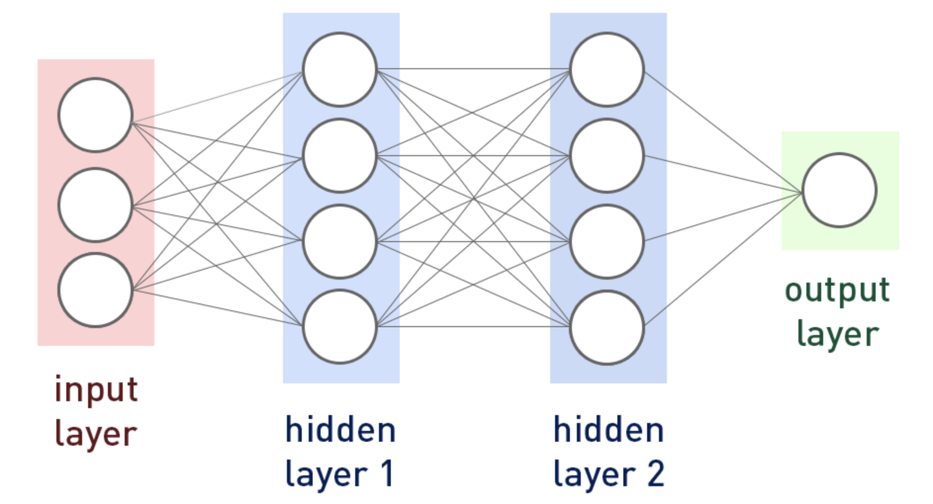
Figure 1: A schematic illustration of a three-layer feedforward neural network.

To solve problem (2.5), we approximate the function $u$ with a feedforward neural network $f^{(L)}$. Thus, the input dimension $d_{0}$ is taken to be the dimension $d$ of the domain $\Omega$, and the output dimension $d_{L}$ is taken to be 1. We denote the set of all such $L$-layer neural networks by $\mathcal{N}\equiv\mathcal{N}(L,N_{\theta},R)$, with $R>0$ being the maximum bound on the network parameters, i.e., all components $|W^{(\ell)}_{i,j}|,\ |b^{(\ell)}_{i}|\leq R$ for all $i,j,\ell$ (or equivalently $\|\theta\|_{\ell^{\infty}}\leq R$, with $\|\cdot\|_{\ell^{\infty}}$ being the Euclidean maximum norm), to explicitly indicate its dependence on the network properties (i.e. depth, total number of parameters and the bound for each parameter).

Now we derive the loss for training neural networks. Let $U(\Omega)$ and $U(\partial\Omega)$ be uniform distributions inside the domain $\Omega$ and on the boundary $\partial\Omega$, respectively. The loss (2.5) can be rewritten as

$$\mathcal{L}_{\gamma}(u)=|\Omega|\mathbb{E}_{U(\Omega)}[a(X)|\nabla u(X)|]+\gamma|\partial\Omega|\mathbb{E}_{U(\partial\Omega)}[a(Y)|Tu(Y)-g|],$$

where $\mathbb{E}_{\mu}$ denotes taking the expectation with respect to a distribution $\mu$. This formulation is commonly known as the population loss in statistical learning theory. The empirical loss $\widehat{\mathcal{L}}_{\gamma}$ takes the form:

$$\widehat{\mathcal{L}}_{\gamma}(\theta)=\frac{|\Omega|}{n_{1}}\sum_{i=1}^{n_{1}}a(X_{i})|\nabla u_{\theta}(X_{i})|+\gamma\frac{|\partial\Omega|}{n_{2}}\sum_{j=1}^{n_{2}}a(Y_{j})|Tu_{\theta}(Y_{j})-g(Y_{j})|,$$ (2.6)

where $u_{\theta}\in\mathcal{N}(L,N_{\theta},R)$ is the neural network realization with parametrization $\theta$, and $\{X_{i}\}^{n_{1}}_{i=1}$ and $\{Y_{j}\}^{n_{2}}_{j=1}$ are $n_{1}$ independent and identically distributed (i.i.d.) training samples drawn from $U(\Omega)$ and $n_{2}$ i.i.d training samples from $U(\partial\Omega)$, respectively. The empirical loss $\widehat{\mathcal{L}}_{\gamma}(\theta)$ is a Monte Carlo approximation of $\mathcal{L}_{\gamma}$. Note that in the low-dimensional case, one may employ standard quadrature rules. Then the training process boils down to solving the following optimization problem:

$$\min_{\theta}\widehat{\mathcal{L}}_{\gamma}({\theta}).$$

Note that the box constraint $\Theta=\{\theta:\|\theta\|_{\ell^{\infty}}\leq R\}$ enforces a compact set on the (finite-dimensional) neural network parameter $\theta$, and the continuity of $\widehat{\mathcal{L}}_{\gamma}$ in $\theta$ (under mild conditions on $\rho$) ensures the existence of a global minimizer to the empirical loss $\widehat{\mathcal{L}}_{\gamma}$. We denote any global minimizer of the empirical loss $\widehat{\mathcal{L}}_{\gamma}(\theta)$ in (2.6) by $\theta^{*}$, and the corresponding neural network approximation in $\mathcal{N}$ by $u_{\theta^{\ast}}$. Note that ${u}_{\theta^{*}}$ is the neural network approximation to the minimizer $u^{*}$ of the population loss $\mathcal{L}_{\gamma}$ in (2.5). However, the empirical loss $\widehat{\mathcal{L}}_{\gamma}(\theta)$ is nonconvex in the parameter $\theta$ and may be fraught with local minimizers, and thus in theory, a global minimizer can be difficult to obtain. Nonetheless, in practice, researchers have found that simple algorithms [14], e.g., (stochastic) gradient descent (SGD) [59] or ADAM [39], can perform fairly well. In practice, the empirical loss $\widehat{\mathcal{L}}_{\gamma}$ is optimized by one such random solver $\mathcal{A}$ (e.g., SGD and ADAM), which outputs a stochastic approximation $\theta_{\mathcal{A}}$ to the optimal $\theta^{*}$ and also the corresponding network $u_{\theta_{\mathcal{A}}}$.

In practical computation, the term $|\nabla u_{\theta}(x)|$ in the loss (2.6) requires some care, since its derivative with respect to the network parameters $\theta$ may be ill-defined when the gradient $\nabla u_{\theta}(x)$ vanishes. Thus we replace the term $|\nabla u_{\theta}(x)|$ with a smooth approximation:

$$\psi(|\nabla u_{\theta}|)=\begin{cases}|\nabla u_{\theta}|,&\quad|\nabla u_{\theta}|\geq\zeta,\\ \frac{|\nabla u_{\theta}|^{2}}{2\zeta}+\frac{\zeta}{2},&\quad\mbox{otherwise},\end{cases}$$ (2.7)

where $\zeta>0$ is a small constant controlling the amount of smoothing. The boundary term can be treated similarly. In practice, the gradient $\nabla u_{\theta}$ with respect to the spatial variable $x$ is computed using automatic differentiation techniques, which are implemented in many popular platforms, e.g., tensorflow module tf.gradients. Thus, the overall computational technique can fully capitalize on modern algorithmic innovations, e.g., automatic differentiation [11].

3 Convergence analysis

Now we present a preliminary analysis of the neural network approximation $u_{\theta_{\mathcal{A}}}$. In the analysis, we take the domain $\Omega$ to be the unit hypercube $\Omega\subset(0,1)^{d}\subset\mathbb{R}^{d}$, and since the parameter $\gamma$ is fixed in the analysis, we suppress it from the notation and denote $\mathcal{L}_{\gamma}$ and $\widehat{\mathcal{L}}_{\gamma}$ by $\mathcal{L}$ and $\widehat{\mathcal{L}}$, respectively. Let ${u}_{\widehat{\theta}}$ be the minimizer of the empirical loss $\widehat{\mathcal{L}}(\theta)$, and let $u_{\theta_{\mathcal{A}}}$ be the optimal network approximation to the minimizer $u^{\ast}$ of the functional $\mathcal{L}$ obtained by a randomized optimizer $\mathcal{A}$. The main aim is to bound the quantity $\mathcal{L}(u_{\theta_{\mathcal{A}}})-\mathcal{L}(u^{\ast})$, which is also known as the generalization error in statistical learning theory [63]. The following lemma gives a crucial decomposition of the generalization error.

Lemma 3.1.

The generalization error $\mathcal{L}(u_{\theta_{\mathcal{A}}})-\mathcal{L}(u^{\ast})$ can be decomposed into

$$\mathcal{L}(u_{\theta_{\mathcal{A}}})-\mathcal{L}(u^{\ast})\leq\underbrace{[\mathcal{L}(\bar{u})-\mathcal{L}(u^{\ast})]}_{\mathcal{E}_{approx}}+2\underbrace{\sup_{u\in\mathcal{N}}|\mathcal{L}(u)-\mathcal{\widehat{L}}(u)|}_{\mathcal{E}_{stats}}+\underbrace{[\mathcal{\widehat{L}}(u_{\theta_{\mathcal{A}}})-\mathcal{\widehat{L}}({u}_{\widehat{\theta}})]}_{\mathcal{E}_{opt}},$$

where $\bar{u}$ is any element in the network class $\mathcal{N}$.

Proof.

Since ${u}_{\widehat{\theta}}$ is the minimizer of $\widehat{\mathcal{L}}$, we have

$$\widehat{\mathcal{L}}({u}_{\widehat{\theta}})-\widehat{\mathcal{L}}(\bar{u})\leq 0,\quad\forall\bar{u}\in\mathcal{N}.$$

Consequently, by adding and subtracting terms, we deduce

$$\mathcal{L}(u_{\theta_{\mathcal{A}}})-\mathcal{L}(u^{\ast}) =\left[\mathcal{L}(u_{\theta_{\mathcal{A}}})-\widehat{\mathcal{L}}(u_{\theta_{\mathcal{A}}})\right]+\left[\widehat{\mathcal{L}}(u_{\theta_{\mathcal{A}}})-\widehat{\mathcal{L}}({u}_{\widehat{\theta}})\right]$$

$$\qquad+\left[\widehat{\mathcal{L}}({u}_{\widehat{\theta}})-\widehat{\mathcal{L}}(\bar{u})\right]+\left[\widehat{\mathcal{L}}(\bar{u})-\mathcal{L}(\bar{u})\right]+\left[\mathcal{L}(\bar{u})-\mathcal{L}(u^{\ast})\right]$$

$$\leq\left[\mathcal{L}(\bar{u})-\mathcal{L}(u^{\ast})\right]+2\sup_{u\in\mathcal{N}}|\mathcal{L}(u)-\mathcal{\widehat{L}}(u)|+\left[\widehat{\mathcal{L}}(u_{\theta_{\mathcal{A}}})-\widehat{\mathcal{L}}({u}_{\widehat{\theta}})\right].$$

This completes the proof of the lemma. ∎

By Lemma 3.1, the generalization error $\mathcal{L}(u_{\theta_{\mathcal{A}}})-\mathcal{L}(u^{\ast})$ can be decomposed into three terms, i.e., approximation error $\mathcal{E}_{approx}$, statistical error $\mathcal{E}_{stat}$, and optimization error $\mathcal{E}_{opt}$. The error $\mathcal{E}_{approx}$ arises because we restrict the sought-for function within the set $\mathcal{N}$, instead of the whole space $BV_{a}(\Omega)$. The error $\mathcal{E}_{stat}$ is the quadrature error arising when approximating the population loss $\mathcal{L}$ with the empirical loss $\widehat{\mathcal{L}}$. The error $\mathcal{E}_{opt}$ arises from the fact that the optimizer we employ may not find a global minimizer. The error $\mathcal{E}_{opt}$ remains very challenging to analyze, due to the non-convexity nature of the optimization problem. Thus, we shall assume that the network is well trained and ignore the optimization error $\mathcal{E}_{opt}$. Note that the functional $\mathcal{L}$ is only convex in $u$ but not strictly so. Hence a bound on the state approximation $u^{*}-u_{\theta_{\mathcal{A}}}$ does not follow directly. Below we analyze the approximation error $\mathcal{E}_{approx}$ and statistical error $\mathcal{E}_{opt}$, in the following two parts separately.

3.1 Approximation error

First we analyze the approximation error $\mathcal{E}_{approx}$, under certain a priori regularity assumption $u^{\ast}\in W^{2,1}(\Omega)$ on the minimizer $u^{*}$ to the loss $\mathcal{L}$. Note that since any neural network function $\bar{u}\in\mathcal{N}$ is differentiable (with respect to the input variable $x$), and also the minimizer $u^{*}$ is differentiable, the distributional derivative $Du$ actually coincides with $\nabla u$. Now we fix any $\bar{u}\in\mathcal{N}$, and let $v=\bar{u}-u^{\ast}$. Then by the triangle inequality and the definition of the loss $\mathcal{L}$, we have

$$\mathcal{L}(\bar{u}) =\int_{\Omega}a(x)|\nabla v(x)+\nabla u^{\ast}(x)|\ \mathrm{d}x+\gamma\int_{\partial\Omega}a(x)|T(v+u^{\ast})-g|\ \mathrm{d}s$$

$$\leq\int_{\Omega}a(x)(|\nabla v(x)|+|\nabla u^{\ast}(x)|)\ \mathrm{d}x+\gamma\Big{(}\int_{\partial\Omega}a(x)|Tu^{\ast}-g|\mathrm{d}s+\int_{\partial\Omega}a(x)|Tv|\mathrm{d}s\Big{)}$$

$$=\mathcal{L}(u^{\ast})+\int_{\Omega}a(x)|\nabla v(x)|\ \mathrm{d}x+\gamma\int_{\partial\Omega}a(x)|Tv(x)|\mathrm{d}s.$$

By Assumption 2.1, $a(x)$ is bounded by $\alpha_{1}$. Moreover, by the trace theorem [23], we have

$$\|Tv\|_{L^{1}(\partial\Omega)}\leq C_{\rm em}\|v\|_{W^{1,1}(\Omega)},$$

where $C_{\rm em}>0$ is the embedding constant from $W^{1,1}(\Omega)$ into $L^{1}(\partial\Omega)$. Consequently,

$$\mathcal{L}(\bar{u})-\mathcal{L}(u^{\ast}) \leq\alpha_{1}\|v\|_{W^{1,1}(\Omega)}+\alpha_{1}\gamma C_{\rm em}\|v\|_{W^{1,1}(\Omega)}$$

$$=\alpha_{1}(1+C_{\rm em}\gamma)\|\bar{u}-u^{\ast}\|_{W^{1,1}(\Omega)}.$$ (3.1)

To bound $\|\bar{u}-u^{\ast}\|_{W^{1,1}(\Omega)}$, we employ the neural network approximation theory from [26]. The main idea is to approximate $u^{\ast}$ by localized Taylor polynomials, where the localization is realized by partition of unity (PU), and the polynomials are then approximated by neural networks. Let $\mathbbm{1}_{[0,1]^{d}}$ be the characteristic function of the domain $[0,1]^{d}$. Note that there is no canonical way to build a PU exactly by neural networks with general activation functions other than ReLU. Gühring and Raslan [26] proposed to approximate $\mathbbm{1}_{[0,1]^{d}}$ with bump functions defined by admissible activation functions with exponential or polynomial decay property. For the analysis below, we assume that the nonlinear activation function $\rho$ is admissible in the following sense [26, Definition 4.2].

Definition 3.1.

Let $j\in\mathbb{N}$. The nonlinear activation function $\rho:\mathbb{R}\to\mathbb{R}$ satisfies

• $\rho$ and $\rho^{\prime}$ are uniformly bounded by $\rho_{0}$ and $\rho_{1}>0$, respectively.

• $\rho$ and $\rho^{\prime}$ are $\eta_{0}$- and $\eta_{1}$-Lipschitz, respectively.

• There exists $I>0$ with $\rho\in C^{j}(\mathbb{R}\backslash[-I,I])$ and $\rho^{\prime}\in W^{j-1,\infty}(\mathbb{R})$, if $j\geq 1$.

Let $\tau=\{0,1\}$ be the order of PU. $\rho$ is said to be exponential (polynomial) $(j,\tau)$-PU-admissible, if additionally there exist $A=A(\rho),\ B=B(\rho)\in\mathbb{R}$, with $A<B$, some $C=C(\rho,j)>0$ and $D=D(\rho,j)>0$, such that

• $|B-\rho^{(\tau)}(x)|\leq Ce^{-Dx}$ ($Cx^{-D}$ if polynomial) for all $x>I$;

• $|A-\rho^{(\tau)}(x)|\leq Ce^{Dx}$ ($C|x|^{-D}$ if polynomial) for all $x<-I$;

• $|\rho^{(k)}(x)|\leq Ce^{-D|x|}$ ($C|x|^{-D}$ if polynomial) for all $x\in\mathbb{R}\backslash[-I,I]$ and all $k=\tau+1,...,j$.

Remark 3.1.

For $\tau=0$, $\rho$ is approximately piecewise constant outside of a neighborhood of zero (e.g., sigmoid) and for $\tau=1$, $\rho$ is approximately piecewise affine-linear outside of a neighborhood of zero (e.g., exponential linear unit). In particular $\arctan$ and inverse square root unit are polynomial PU-admissible, and $\tanh$ and sigmoid are exponential PU-admissible.

Now we state the approximation theorem [26, Proposition 4.8].

Theorem 3.1.

Let $d\in\mathbb{N}$, $j,\tau\in\mathbb{N}_{0}$, $k\in\{0,\cdots,j\}$, $n\geq k+1$, $1\leq p\leq\infty$, and $\mu>0$. Let $\mathcal{F}_{n,d,p}:=\{f\in W^{n,p}((0,1)^{d}):\|f\|_{W^{n,p}((0,1)^{d})}\leq 1\}$. Suppose that $\rho(x)$ is an exponential (polynomial) $(j,\tau)$-PU admissible activation function, and there exists $x_{0}\in\mathbb{R}$ such that $\rho$ is three times continuously differentiable in a neighborhood of $x_{0}$. Then for any $\epsilon>0$ and for any $f\in\mathcal{F}_{n,d,p}$, there exists a neural network $f_{NN}$ with depth at most $\ C\log(d+n)$ and at most

$$N_{\theta}=\left\{\begin{aligned} C\epsilon^{-\frac{d}{n-k-\mu(k=2)}},&\quad\mbox{if $\rho$ is exponential admissible},\\ C\epsilon^{-\frac{d}{n-k}},&\quad\mbox{if $\rho$ is polynomial admissible},\end{aligned}\right.$$

non-zero weights, where $\mu\in(0,1)$ is small, such that

$$\|f-f_{NN}\|_{W^{k,p}([0,1]^{d})}\leq\epsilon.$$

Moreover, the weights in the neural network are bounded in absolute value by

$$\left\{\begin{aligned} C(d,n,p,k)\epsilon^{-2-\frac{2(d/p+d+k+\mu(k=2))+d/p+d}{n-k-\mu(k=2)}},&\quad\mbox{if $\rho$ is exponential admissible},\\ C(d,n,p,k)\epsilon^{-2-\frac{2(d/p+d+k)+d/p+d}{n-k}},&\quad\mbox{if $\rho$ is polynomial admissible}.\end{aligned}\right.$$

To bound the approximation error (3.1), we apply Theorem 3.1 with $k=p=1$ and $n=2$. Then for any $\epsilon>0$ and any $f\in W^{2,1}([0,1]^{d})$ such that $\|f\|_{W^{2,1}((0,1)^{d})}\leq 1$, there exists a neural network $\bar{f}$ with $\bar{c_{1}}(d)\log(d+2)$ layers and $\bar{c_{2}}(d)\epsilon^{-\frac{d}{1-\mu}}$ (or $\bar{c_{2}}(d)\epsilon^{-d}$, if $\rho$ is polynomial admissible) number of network parameters each bounded by $\bar{c_{3}}(d)\epsilon^{-\frac{4+6d}{1-\mu}}$ (or $\bar{c}_{3}(d)\epsilon^{-(4+6d)}$ if $\rho$ is polynomial admissible), such that

$$\|\ f-\bar{f}\ \|_{W^{1,1}([0,1]^{d})}\leq\epsilon.$$

The following proposition records the approximation result.

Proposition 3.1.

Let the minimizer $u^{\ast}$ to the functional $\mathcal{L}$ satisfies $u^{\ast}\in{W^{2,1}(\Omega)}$, and let $\rho$ be the nonlinear activation function. Then for any $\epsilon>0$, there exists a network work class

$$\mathcal{N}=\left\{\begin{aligned} \mathcal{N}(c_{1}\log(d+2),c_{2}\epsilon^{-\frac{d}{1-\mu}},c_{3}\epsilon^{-\frac{4+6d}{1-\mu}}),&\quad\mbox{if $\rho$ is exponential admissible},\\ \mathcal{N}(c_{1}\log(d+2),c_{2}\epsilon^{-d},\ c_{3}\epsilon^{-(4+6d)}),&\quad\mbox{if $\rho$ is polynomial admissable},\end{aligned}\right.$$

with $\mu\in(0,1)$ being an arbitrarily small positive number, such that there exists a $\bar{u}\in\mathcal{N}$ with

$$\|u^{\ast}-\bar{u}\|_{W^{1,1}(\Omega)}\leq C\epsilon,$$

with the constant $C$ depending on $\|u^{*}\|_{W^{2,1}(\Omega)}$. In particular, there exists a neural network $\bar{u}\in\mathcal{N}$ such that

$$\mathcal{L}(\bar{u})-\mathcal{L}(u^{\ast})\leq C\alpha_{1}(1+C_{\rm em}\gamma)\epsilon.$$

Proof.

By Sobolev extension theorem [23] and the assumption $u^{*}\in W^{2,1}(\Omega)$, since $\Omega\subset(0,1)^{d}$, there exists a bounded extension of $u^{*}$ from $\Omega$ to $(0,1)^{d}$, denoted by $Eu^{*}$ such that

$$\|Eu^{*}\|_{W^{2,1}((0,1)^{d})}\leq C\|u^{*}\|_{W^{2,1}(\Omega)}.$$

Then by Theorem 3.1, we can find a neural network $u^{*}\in\mathcal{N}$ satisfies the desired approximation for the function $Eu^{*}/\|Eu^{*}\|_{W^{2,1}((0,1)^{d})}$. Then the desired assertion follows directly. ∎

Remark 3.2.

In Proposition 3.1, we have assumed the existence of a minimizer $u^{*}\in W^{2,1}(\Omega)$ to the loss $\mathcal{L}$. This assumption may be relaxed to an approximate minimizer $u^{\epsilon}\in W^{2,1}(\Omega)$ such that $\mathcal{L}(u^{\epsilon})-\inf_{u\in BV_{a}(\Omega)}\mathcal{L}(u)\leq\epsilon$. However, the $W^{2,1}(\Omega)$ norm of $u^{\epsilon}$ may depend on the tolerance $\epsilon$, which obscures the dependence between the network parameters and the error tolerance $\epsilon$.

3.2 Statistical Error

In this part, we bound the statistical error $\sup_{u\in\mathcal{N}}\lvert\mathcal{L}(u)-\widehat{\mathcal{L}}(u)\rvert$. To this end, we define

$$\mathcal{L}_{1}(u)=|\Omega|\mathbb{E}_{X\sim U(\Omega)}[a(X)|\nabla u(X)|],\quad\widehat{\mathcal{L}}_{1}(\bar{u})=\frac{|\Omega|}{n_{1}}\sum_{i=1}^{n_{1}}a(X_{i})|\nabla\bar{u}(X_{i})|,$$

$$\mathcal{L}_{2}(u)=\gamma|\partial\Omega|\mathbb{E}_{Y\sim U(\partial\Omega)}[a(Y)|Tu(Y)-g(Y)|],\quad\widehat{\mathcal{L}}_{2}(\bar{u})=\gamma\frac{|\partial\Omega|}{n_{2}}\sum_{j=1}^{n_{2}}a(Y_{j})|T\bar{u}(Y_{j})-g(Y_{j})|.$$

Then by the triangle inequality, we have

$$\sup_{u\in\mathcal{N}}|\mathcal{L}(u)-\widehat{\mathcal{L}}(u)|\leq\sum_{i=1}^{2}\sup_{u\in\mathcal{N}}|\mathcal{L}_{i}(u)-\mathcal{\widehat{L}}_{i}(u)|.$$

Below we denote both $U(\Omega)$ and $U(\partial\Omega)$ by $\mu$, and set $n=n_{1}$ and $n=n_{2}$ accordingly. Hence, there are $n$ i.i.d samples drawn from $\mu$, denoted by $Z_{n}=\{z_{i}\}_{i=1}^{n}$ with $z_{i}\sim\mu$. We analyze $\mathbb{E}_{Z_{n}}[\sup_{u\in\mathcal{N}}|\mathcal{L}_{1}(u)-\mathcal{\widehat{L}}_{1}(u)|]$ and $\mathbb{E}_{Z_{n}}[\sup_{u\in\mathcal{N}}|\mathcal{L}_{2}(u)-\mathcal{\widehat{L}}_{2}(u)|]$ separately. The concept of Rademacher complexity plays a crucial role in the analysis. Rademacher complexity $\mathcal{R}_{n}(\mathcal{F})$ measures the capacity of a function class $\mathcal{F}$ restricted on $n$ random samples $Z_{n}$ [10, 9]. For many function classes, the Rademacher complexity is known. For example, see [43, Theorem 3] for the class of two-layer neural networks.

Definition 3.2.

The Rademacher complexity $\mathfrak{R}_{n}(\mathcal{F})$ of a function class $\mathcal{F}$ is defined by

$$\mathfrak{R}_{n}(\mathcal{F})=\mathbb{E}_{Z_{n},\Sigma_{n}}\bigg{[}\sup_{u\in\mathcal{F}}\ \frac{1}{n}\bigg{\lvert}\ \sum_{i=1}^{n}\sigma_{i}u(z_{i})\ \bigg{\rvert}\bigg{]},$$

where $\Sigma_{n}=\{\sigma_{i}\}_{i=1}^{n}$ are $n$ i.i.d Rademacher variables, i.e., with probability $P(\sigma_{i}=1)=P(\sigma_{i}=-1)=\frac{1}{2}$.

Given an $L$-layer neural network class $\mathcal{N}$, we define an associated function class

$$\mathcal{G}=\big{\{}g:[0,1]^{d}\rightarrow\mathbb{R}\mbox{ such that }g(x)=|\nabla u(x)|,\ \ \forall x\in[0,1]^{d},\mbox{ with }u\in\mathcal{N}\big{\}}.$$

Recall that $|\nabla u(x)|$ denotes the Euclidean norm of the gradient vector $(\partial_{x_{1}}u,\ldots,\partial_{x_{d}}u)^{t}\in\mathbb{R}^{d}$. First, we bound $\mathbb{E}_{Z_{n}}[\sup_{u\in\mathcal{N}}|\mathcal{L}_{1}(u)-\mathcal{\widehat{L}}_{1}(u)|]$ in terms of the Rademacher complexity $\mathfrak{R}_{n}(\mathcal{G})$. The proof is based on a standard symmetrization argument (see, e.g., [46, Theorem 14]), and it is included only for completeness.

Lemma 3.2.

The following bound holds

$$\mathbb{E}_{Z_{n}}\Big{[}\sup_{u\in\mathcal{N}}|\mathcal{L}_{1}(u)-\mathcal{\widehat{L}}_{1}(u)|\Big{]}\leq 2\alpha_{1}|\Omega|\mathfrak{R}_{n}(\mathcal{G}).$$

Proof.

We denote ${\rm I}=\mathbb{E}_{Z_{n}}[\sup_{u\in\mathcal{N}}|\mathcal{L}_{1}(u)-\mathcal{\widehat{L}}_{1}(u)|]$. By the definitions of $\mathcal{L}_{1}$, $\mathcal{\widehat{L}}_{1}$, $\mu$ and $Z_{n}$, we have

$${\rm I} =\mathbb{E}_{Z_{n}}\Big{[}\sup_{u\in\mathcal{N}}\Big{|}|\Omega|\mathbb{E}_{\mu}[a(Z)|\nabla u(Z)|]-\frac{|\Omega|}{n}\sum_{i=1}^{n}a(z_{i})|\nabla u(z_{i})|\Big{|}\Big{]}$$

$$=\frac{|\Omega|}{n}\mathbb{E}_{Z_{n}}\Big{[}\sup_{u\in\mathcal{N}}\Big{|}n\mathbb{E}_{\mu}[a(Z)|\nabla u(Z)|]-\sum_{i=1}^{n}a(z_{i})|\nabla u(z_{i})|\Big{|}\Big{]}$$

$$=\frac{|\Omega|}{n}\mathbb{E}_{Z_{n}}\Big{[}\sup_{u\in\mathcal{N}}\Big{|}\sum_{i=1}^{n}\mathbb{E}_{\tilde{Z}_{n}}[a(\tilde{z_{i}})|\nabla u(\tilde{z_{i}})|]-\sum_{i=1}^{n}a(z_{i})|\nabla u(z_{i})|\Big{|}\Big{]},$$

where $\tilde{Z}_{n}=\{\tilde{z}_{i}\}_{i=1}^{n}$ denotes $n$ independent samples from the distribution $\mu$, independent from $Z_{n}$. Since $\sup(\cdot)$ is a convex function, by Jensen’s inequality, we deduce

$${\rm I}\leq\frac{|\Omega|}{n}\mathbb{E}_{Z_{n},\tilde{Z}_{n}}\Big{[}\sup_{u\in\mathcal{N}}\Big{|}\sum_{i=1}^{n}\big{(}a(\tilde{z_{i}})|\nabla u(\tilde{z_{i}})|-a(z_{i})|\nabla u(z_{i})|)\Big{|}\Big{]}.$$

Since $z_{i}$ and $\tilde{z}_{i}$ are i.i.d., the distribution of the supremum is unchanged when we swap them. One may insert any $\{\sigma_{i}\}\in\{\pm 1\}^{n}$, in particular, the expectation of the supremum is unchanged. Since this is true for any $\sigma_{i}$, we can take the expectation over any random choice of the $\sigma_{i}$. Thus, we deduce

$${\rm I}\leq\frac{|\Omega|}{n}\mathbb{E}_{Z_{n},\tilde{Z}_{n},\Sigma_{n}}\Big{[}\sup_{u\in\mathcal{N}}\Big{|}\sum_{i=1}^{n}\sigma_{i}\big{(}a(\tilde{z_{i}})|\nabla u(\tilde{z_{i}})|-a(z_{i})|\nabla u(z_{i})|\big{)}\Big{|}\Big{]}.$$

Then by the triangle inequality, we have

$$\begin{split}{\rm I}&\leq\frac{|\Omega|}{n}\mathbb{E}_{Z_{n},\tilde{Z}_{n},\Sigma_{n}}\Big{[}\sup_{u\in\mathcal{N}}\Big{|}\sum_{i=1}^{n}\sigma_{i}a(\tilde{z_{i}})|\nabla u(\tilde{z_{i}})|\Big{|}+\sup_{u\in\mathcal{N}}\Big{|}\sum_{i=1}^{n}\sigma_{i}a(z_{i})|\nabla u(z_{i})|\Big{|}\Big{]}\\ &=\frac{|\Omega|}{n}\mathbb{E}_{\tilde{Z}_{n},\Sigma_{n}}\Big{[}\sup_{u\in\mathcal{N}}\Big{|}\sum_{i=1}^{n}\sigma_{i}a(\tilde{z_{i}})|\nabla u(\tilde{z_{i}})|\Big{|}\Big{]}+\frac{|\Omega|}{n}\mathbb{E}_{Z_{n},\Sigma_{n}}\Big{[}\sup_{u\in\mathcal{N}}\Big{|}\sum_{i=1}^{n}\sigma_{i}a(z_{i})|\nabla u(z_{i})|\Big{|}\Big{]}\\ &=2|\Omega|\mathbb{E}_{Z_{n},\Sigma_{n}}\Big{[}\sup_{u\in\mathcal{N}}\ \frac{1}{n}\Big{|}\sum_{i=1}^{n}\sigma_{i}a(z_{i})|\nabla u(z_{i})|\Big{|}\Big{]}.\end{split}$$

Now by Assumption 2.1, we have $a\leq\alpha_{1}$ a.e. $\Omega$ and by the multiplicative inequality of Rademacher complexity, we obtain

$${\rm I}\leq 2\alpha_{1}|\Omega|\mathbb{E}_{Z_{n},\Sigma_{n}}\Big{[}\sup_{u\in\mathcal{N}}\ \frac{1}{n}\Big{|}\sum_{i=1}^{n}\sigma_{i}|\nabla u(z_{i})|\Big{|}\Big{]}=2\alpha_{1}|\Omega|\mathfrak{R}(\mathcal{G}).$$

This completes the proof of the lemma. ∎

By Lemma 3.2, it suffices to bound the Rademacher complexity $\mathcal{R}_{n}(\mathcal{G})$ of the function class $\mathcal{G}$. This can be achieved using Dudley’s formula from the theory of empirical process [69]. First we recall the covering number of a function class.

Definition 3.3.

Let $(X,{\rho})$ be a metric space. An $\epsilon$-cover of a set $A\subset X$ with respect to the metric $\rho$ is a collection of points $\{x_{i}\}_{i=1}^{n}\subset A$ such that for every $x\in A$, there exists $i\in\{1,\cdots,n\}$ such that $\rho(x,x_{i})\leq\epsilon$. The $\epsilon$-covering number $\mathcal{C}(A,\rho,\epsilon)$ is the cardinality of the smallest $\epsilon$-cover of $A$ with respect to the metric $\rho$.

The Rademacher complexity $\mathcal{R}_{n}(\mathcal{G})$ is related to the covering number $\mathcal{C}(\mathcal{G},\|\cdot\|_{L^{\infty}(\Omega)},\epsilon)$ by the refined Dudley’s formula [20] (see, e.g., [65, 60] for the current form). Note that the statement is slightly different from the standard Dudley’s theorem where the covering number is based on the empirical $\ell^{2}$-metric instead of the $L^{\infty}(\Omega)$-metric. However, the $L^{\infty}(\Omega)$ metric is stronger than the empirical $\ell^{2}$ metric, and the covering number is monotonically increasing with respect to the metric [60, Lemma 2]. The lemma follows directly from the classical Dudley’s theorem.

Lemma 3.3.

The Rademacher complexity $\mathfrak{R}_{n}(\mathcal{G})$ of a function class $\mathcal{G}$ is bounded by

$$\mathfrak{R}_{n}(\mathcal{G})\leq\inf_{0<\delta<M}\bigg{(}4\delta\ +\ \frac{12}{\sqrt{n}}\int^{M}_{\delta}\sqrt{\log\mathcal{C}(\mathcal{G},\|\cdot\|_{L^{\infty}(\Omega)},\epsilon)}\ d\epsilon\bigg{)},$$

where $\mathcal{C}(\mathcal{G},\|\cdot\|_{L^{\infty}(\Omega)},\epsilon)$ is the covering number of the set $\mathcal{G}$, and $M:=\sup_{g\in\mathcal{G}}\|g\|_{L^{\infty}(\Omega)}$.

Next we bound the covering number $\mathcal{C}(\mathcal{G},\|\cdot\|_{L^{\infty}(\Omega)},\epsilon)$ of the set $\mathcal{G}$. This is based on the Lipschitz continuity of functions in the set $\mathcal{G}$ with respect to the network parameter $\theta$. For $g,\ \tilde{g}\in\mathcal{G}$, there exist two neural networks $f^{(L)}$ and $\tilde{f}^{(L)}$ (with the corresponding network parameters being $\theta=\{W^{(\ell)},b^{(\ell)}\}_{\ell=1}^{L}$ and $\tilde{\theta}=\{\tilde{W}^{(\ell)},\tilde{b}^{(\ell)}\}_{\ell=1}^{L}$) such that $f^{(L)}$ and $\tilde{f}^{(L)}$ can be written as

$$f^{(L)} =W^{(L)}\rho(W^{(L-1)}\rho(W^{(L-2)}\cdots+b^{(L-2)})+b^{(L-1)})+b^{(L)},$$

$$\tilde{f}^{(L)} =\tilde{W}^{(L)}\rho(\tilde{W}^{(L-1)}\rho(\tilde{W}^{(L-2)}\cdots+\tilde{b}^{(L-2)})+\tilde{b}^{(L-1)})+\tilde{b}^{(L)},$$

and accordingly

$$g(x)=|\nabla f^{(L)}(x)|\quad\mbox{and}\quad\tilde{g}(x)=|\nabla\tilde{f}^{(L)}(x)|.$$

To indicate the dependence of $g$ on $\theta$, we write $g_{\theta}$ below. To bound the covering number $\mathcal{C}(\mathcal{G},\|\cdot\|_{L^{\infty}(\Omega)},\epsilon)$ of $\mathcal{G}$, we bound $\|g_{\theta}-\tilde{g}_{\tilde{\theta}}\|_{L^{\infty}(\Omega)}$ in terms of $\|\theta-\tilde{\theta}\|_{\ell^{\infty}}$. Meanwhile, we have

$$\|g_{\theta}-\tilde{g}_{\tilde{\theta}}\|_{L^{\infty}(\Omega)}=\||\nabla f^{(L)}|-|\nabla\tilde{f}^{(L)}|\|_{L^{\infty}(\Omega)}\leq\||\nabla(f^{(L)}-\tilde{f}^{(L)})|\|_{L^{\infty}(\Omega)}.$$ (3.2)

Thus, it suffices to bound the partial derivatives $\|\partial_{x_{i}}(f^{(L)}-\tilde{f}^{(L)})\|_{L^{\infty}(\Omega)}$, for $i=1,2,\cdots,d$. The next lemma gives the requisite estimates (as well as auxiliary estimates). Note that under different assumptions (i.e., boundedness assumptions on the activation function, different norms on the parameters, or evaluation of the neural networks on input data), similar approaches can be found in [3, 8, 12].

Lemma 3.4.

Let the activation function $\rho$ satisfy the conditions (i)–(ii) in Definition 3.1, $\mathcal{W}$ be the width of the network class, and $R$ the $\ell^{\infty}$ bound on the network parameters $\theta$. Then with $\rho_{0},\ \rho_{1},\ \eta_{0},\ \eta_{1},\ R$ and $\mathcal{W}$, there holds

$$\|\partial_{x_{i}}(f^{(L)}-\tilde{f}^{(L)})\|_{L^{\infty}(\Omega)} \leq L^{2}\rho_{0}\rho_{1}^{L-1}\eta_{1}\eta_{0}^{L-2}R^{2L-2}\mathcal{W}^{2L-2}\|\theta-\tilde{\theta}\|_{\ell^{\infty}},$$ (3.3)

$$\sup_{g\in\mathcal{G}}\|g\|_{L^{\infty}(\Omega)} \leq\sqrt{d}R^{L}(\rho_{1}\mathcal{W})^{L-1}.$$ (3.4)

Proof.

Let $r:=\|\theta-\tilde{\theta}\|_{\ell^{\infty}}$. Recall that $f^{(1)}=\rho(W^{(1)}x+b^{(1)})$, and $f^{(\ell)}=\rho(W^{(\ell)}f^{(\ell-1)}+b^{(\ell)})$, for $\ell=1,2,\cdots,L-1$. We denote the $j$th component of $f^{(\ell)}\in\mathbb{R}^{d_{\ell}}$ by $f^{(\ell)}_{j}$. Noting $W^{(L)}\in\mathbb{R}^{1\times d_{L-1}}$ and $b^{(L)}\in\mathbb{R}$, writing out explicitly $f^{(L)}$ and $\tilde{f}^{(L)}$ and applying the triangle inequality lead to

$$\quad\big{\|}\partial_{x_{i}}(f^{(L)}-\tilde{f}^{(L)})\big{\|}_{L^{\infty}(\Omega)}$$

$$=\Big{\|}\partial_{x_{i}}\bigg{(}\sum_{j=1}^{d_{L-1}}W^{(L)}_{j}f^{(L-1)}_{j}+b^{(L)}\bigg{)}-\partial_{x_{i}}\bigg{(}\sum_{j=1}^{d_{L-1}}\tilde{W}^{(L)}_{j}\tilde{f}^{(L-1)}_{j}+\tilde{b}^{(L)}\bigg{)}\Big{\|}_{L^{\infty}(\Omega)}$$

$$=\Big{\|}\sum_{j=1}^{d_{L-1}}W^{(L)}_{j}\partial_{x_{i}}f^{(L-1)}_{j}-\sum_{j=1}^{d_{L-1}}\tilde{W}^{(L)}_{j}\partial_{x_{i}}\tilde{f}^{(L-1)}_{j}\Big{\|}_{L^{\infty}(\Omega)}$$

$$\leq\sum_{j=1}^{d_{L-1}}\Big{\|}W^{(L)}_{j}\partial_{x_{i}}f^{(L-1)}_{j}-\tilde{W}^{(L)}_{j}\partial_{x_{i}}\tilde{f}^{(L-1)}_{j}\Big{\|}_{L^{\infty}(\Omega)}$$

$$\leq\sum_{j=1}^{d_{L-1}}\big{[}|W^{(L)}_{j}-\tilde{W}^{(L)}_{j}|\|\partial_{x_{i}}f^{(L-1)}_{j}\|_{L^{\infty}(\Omega)}+|\tilde{W}^{(L)}_{j}|\|\partial_{x_{i}}(f^{(L-1)}_{j}-\tilde{f}^{(L-1)}_{j})\|_{L^{\infty}(\Omega)}\big{]}$$

$$\leq r\sum_{j=1}^{d_{L-1}}\|\partial_{x_{i}}f^{(L-1)}_{j}\|_{L^{\infty}(\Omega)}+R\sum_{j=1}^{d_{L-1}}\|\partial_{x_{i}}(f^{(L-1)}_{j}-\tilde{f}^{(L-1)}_{j})\|_{L^{\infty}(\Omega)},$$ (3.5)

in view of the definition of $r$ and the condition $|\tilde{W}_{j}^{(L)}|\leq R$. Thus, to bound $\|\partial_{x_{i}}(f^{(L)}-\tilde{f}^{(L)})\|_{L^{\infty}(\Omega)}$, it suffices to estimate $\|\partial_{x_{i}}f^{(L-1)}_{j}\|_{L^{\infty}(\Omega)}$ and $\|\partial_{x_{i}}(f^{(L-1)}_{j}-\tilde{f}^{(L-1)}_{j})\|_{L^{\infty}(\Omega)}$. We derive the requisite bounds below using mathematical induction. The rest of the proof is elementary but fairly lengthy, and hence we divide it into four steps.

1. Bound $\|\partial_{x_{i}}f_{j}^{(\ell)}\|_{L^{\infty}(\Omega)}$ for $\ell=1,2,\cdots,L-1,\ j=1,2,\cdots,d_{\ell}.$ By the chain rule, we have

   $$\partial_{x_{i}}f_{j}^{(\ell)}=\rho^{\prime}\Big{(}\sum_{k=1}^{d_{\ell-1}}W^{(\ell)}_{jk}f^{(\ell-1)}_{k}+b^{(\ell)}_{j}\Big{)}\sum_{k=1}^{d_{\ell-1}}W^{(\ell)}_{jk}\partial_{x_{i}}f^{(\ell-1)}_{k}.$$

   For the case $\ell=1$, the assumptions $|\rho^{\prime}|\leq\rho_{1}$ (cf. Definition 3.1(i)) and $|W_{ji}^{(1)}|\leq R$ yields

   $$\|\partial_{x_{i}}f_{j}^{(1)}\|_{L^{\infty}(\Omega)} \leq\Big{\|}\rho^{\prime}\Big{(}\sum_{k=1}^{d}W^{(1)}_{jk}x_{k}+b^{(1)}_{j}\Big{)}W^{(1)}_{ji}\Big{\|}_{L^{\infty}(\Omega)}\leq\rho_{1}R.$$

   For $\ell\geq 2$, the triangle inequality and the conditions $|\rho^{\prime}|\leq\rho_{1}$, $|W_{jk}^{(\ell)}|\leq R$ and $d_{\ell-1}\leq\mathcal{W}$ imply

   $$\|\partial_{x_{i}}f_{j}^{(\ell)}\|_{L^{\infty}(\Omega)}\leq\rho_{1}\sum_{k=1}^{d_{\ell-1}}|W^{(\ell)}_{jk}|\|\partial_{x_{i}}f^{(\ell-1)}_{k}\|_{L^{\infty}(\Omega)}\leq\rho_{1}R\mathcal{W}\max_{k}\|\partial_{x_{i}}f^{(\ell-1)}_{k}\|_{L^{\infty}(\Omega)}.$$

   Combining the preceding two estimates directly leads to

   $$\|\partial_{x_{i}}f_{j}^{(\ell)}\|_{L^{\infty}(\Omega)}\leq(\rho_{1}R)^{\ell}\mathcal{W}^{\ell-1},\quad\ell=1,2,\cdots,L-1,\ j=1,2,\cdots,d_{\ell}.$$ (3.6)

2. Bound $\|f^{(\ell)}_{j}-\tilde{f}^{(\ell)}_{j}\|_{L^{\infty}(\Omega)}$ for $\ell=1,2,\cdots,L-1,\ j=1,2,\cdots,d_{\ell}$, assuming $\rho_{0},\ \rho_{1},\ \eta_{0},\ \eta_{1}\geq 1$. For the case $\ell=1$, by the definitions of $f^{(1)}_{j}$ and $\tilde{f}^{(1)}_{j}$, the Lipschitz continuity of $\rho$, and the triangle inequality, we have

   $$\|f^{(1)}_{j}- \tilde{f}^{(1)}_{j}\|_{L^{\infty}(\Omega)}=\Big{\|}\rho\Big{(}\sum_{k=1}^{d}W^{(1)}_{jk}x_{k}+b^{(1)}_{j}\Big{)}-\rho\Big{(}\sum_{k=1}^{d}\tilde{W}^{(1)}_{jk}x_{k}+\tilde{b}^{(1)}_{j}\Big{)}\Big{\|}_{L^{\infty}(\Omega)}$$

   $$\leq\eta_{0}\Big{\|}\sum_{k=1}^{d}W^{(1)}_{jk}x_{k}+b^{(1)}_{j}-\sum_{k=1}^{d}\tilde{W}^{(1)}_{jk}x_{k}-\tilde{b}^{(1)}_{j}\Big{\|}_{L^{\infty}(\Omega)}$$

   $$\leq\eta_{0}\sum_{k=1}^{d}|W^{(1)}_{jk}-\tilde{W}^{(1)}_{jk}|\|x_{k}\|_{L^{\infty}(\Omega)}+\eta_{0}|b^{(1)}_{j}-\tilde{b}^{(1)}_{j}|\leq\eta_{0}r(1+\rho_{0}\mathcal{W}),$$

   in view of the definition $r=\|\theta-\tilde{\theta}\|_{\ell^{\infty}}$ and the trivial estimate $\|x_{p}\|_{L^{\infty}(\Omega)}\leq 1$ for all $p=1,\ldots,d$, since $x\in[0,1]^{d}$. Meanwhile, for the case $\ell\geq 2$, by the Lipschitz continuity of and the uniform bound $\rho_{0}$ on $\rho$, the triangle inequality and the induction hypothesis, we obtain

   $$\|f^{(\ell)}_{j}-\tilde{f}^{(\ell)}_{j}\|_{L^{\infty}(\Omega)} \leq\eta_{0}\Big{\|}\sum_{k=1}^{d_{\ell-1}}W^{(\ell)}_{jk}f^{(\ell-1)}_{k}+b^{(\ell)}_{j}-\sum_{k=1}^{d_{\ell-1}}\tilde{W}^{(\ell)}_{jk}\tilde{f}^{(\ell-1)}_{k}-\tilde{b}^{(\ell)}_{j}\Big{\|}_{L^{\infty}(\Omega)}$$

   $$\leq\eta_{0}|b^{(\ell)}_{j}-\tilde{b}^{(\ell)}_{j}|+\eta_{0}\sum_{k=1}^{d_{\ell-1}}\left[|W^{(\ell)}_{jk}-\tilde{W}^{(\ell)}_{jk}|\|f^{(\ell-1)}_{k}\|_{L^{\infty}(\Omega)}\right.$$

   $$\quad+\left.|\tilde{W}^{(\ell)}_{jk}|\|f^{(\ell-1)}_{k}-\tilde{f}^{(\ell-1)}_{k}\|_{L^{\infty}(\Omega)}\right]$$

   $$\leq\eta_{0}r+\eta_{0}r\rho_{0}d_{\ell-1}+\eta_{0}R\sum_{k=1}^{d_{\ell-1}}\|f^{(\ell-1)}_{k}-\tilde{f}^{(\ell-1)}_{k}\|_{L^{\infty}(\Omega)}$$

   $$\leq\eta_{0}(1+\rho_{0}\mathcal{W})r+\eta_{0}R\mathcal{W}c_{\ell-1}.$$

   with $c_{\ell}=\max_{k}\|f^{(\ell)}_{k}-\tilde{f}^{(\ell)}_{k}\|_{L^{\infty}(\Omega)}$. Then the preceding inequality implies

   $$c_{\ell}\leq\eta_{0}(1+\rho_{0}\mathcal{W})r+\eta_{0}R\mathcal{W}c_{\ell-1}.$$

   By repeatedly applying the inequality and using the bound on $c_{1}$, we arrive at

   $$c_{\ell}\leq\eta_{0}r(1+\rho_{0}\mathcal{W})\big{(}1+\ldots+(\eta_{0}R\mathcal{W})^{\ell-1}\big{)}.$$

   In particular, we directly obtain (for $\eta_{0},R,\mathcal{W}\geq 1$)

   $$\|f^{(\ell)}_{j}-\tilde{f}^{(\ell)}_{j}\|_{L^{\infty}(\Omega)}\leq 2\ell\rho_{0}\eta_{0}^{\ell}\mathcal{W}^{\ell}R^{\ell-1}r,\quad\ell=1,2,\cdots,L-1,\ j=1,2,\cdots,d_{\ell}.$$ (3.7)

3. Bound the term $D_{j}^{(\ell)}:=\|\rho^{\prime}(\sum_{k=1}^{d_{\ell-1}}W^{(\ell)}_{jk}f^{(\ell-1)}_{k}+b^{(\ell)}_{j})-\rho^{\prime}(\sum_{k=1}^{d_{\ell-1}}\tilde{W}^{(\ell)}_{jk}\tilde{f}^{(\ell-1)}_{k}+\tilde{b}^{(\ell)}_{j})\|_{L^{\infty}(\Omega)}$. By the Lipschitz continuity of $\rho^{\prime}$, the triangle inequality, and the bounds $|\rho|\leq\rho_{0}$ and $d_{\ell-1}\leq\mathcal{W}$, we have

   $$D_{j}^{(\ell)} \leq\eta_{1}\Big{\|}\sum_{k=1}^{d_{\ell-1}}W^{(\ell)}_{jk}f^{(\ell-1)}_{k}+b^{(\ell)}_{j}-\sum_{k=1}^{d_{\ell-1}}\tilde{W}^{(\ell)}_{jk}\tilde{f}^{(\ell-1)}_{k}-\tilde{b}^{(\ell)}_{j}\Big{\|}_{L^{\infty}(\Omega)}$$

   $$\leq\eta_{1}|b^{(\ell)}_{j}-\tilde{b}^{(\ell)}_{j}|+\eta_{1}\sum_{k=1}^{d_{\ell-1}}\left[|W^{(\ell)}_{jk}-\tilde{W}^{(\ell)}_{jk}|\|f^{(\ell-1)}_{k}\|_{L^{\infty}(\Omega)}\right.$$

   $$\quad\left.+|\tilde{W}^{(\ell)}_{jk}|\|f^{(\ell-1)}_{k}-\tilde{f}^{(\ell-1)}_{k}\|_{L^{\infty}(\Omega)}\right]$$

   $$\leq\eta_{1}r(1+\rho_{0}\mathcal{W})+\eta_{1}R\mathcal{W}\max_{k}\|f^{(\ell-1)}_{k}-\tilde{f}^{(\ell-1)}_{k}\|_{L^{\infty}(\Omega)}.$$

   This and the bound (3.7) imply

   $$D_{j}^{(\ell)}\leq 2\ell\rho_{0}\eta_{1}\eta_{0}^{\ell-1}\mathcal{W}^{\ell}R^{\ell-1}r.$$ (3.8)

4. Bound $P_{ij}^{(\ell)}:=\|\partial_{x_{i}}(f^{(\ell)}_{j}-\tilde{f}^{(\ell)}_{j})\|_{L^{\infty}(\Omega)}$ for $\ell=1,2,\cdots,L-1$, $j=1,\cdots,d_{\ell}$. We claim

   $$P^{(\ell)}_{ij}\leq\ell(\ell+2)\rho_{0}\rho_{1}^{\ell}\eta_{1}\eta_{0}^{\ell-1}(R\mathcal{W})^{2\ell-1}r,\quad\ell=1,2,\cdots,L-1,\ j=1,\cdots,d_{\ell}.$$ (3.9)

   For the case $\ell=1$, the chain rule and the triangle inequality give

   $$P_{ij}^{(1)} =\Big{\|}\rho^{\prime}\Big{(}\sum_{k=1}^{d}W^{(1)}_{jk}x_{k}+b^{(1)}_{j}\Big{)}W^{(1)}_{ji}-\rho^{\prime}\Big{(}\sum_{k=1}^{d}\tilde{W}^{(1)}_{jk}x_{k}+\tilde{b}^{(1)}_{j}\Big{)}\tilde{W}^{(1)}_{ji}\Big{\|}_{L^{\infty}(\Omega)}$$

   $$\leq\Big{\|}\rho^{\prime}\Big{(}\sum_{k=1}^{d}W^{(1)}_{jk}x_{k}+b^{(1)}_{j}\Big{)}-\rho^{\prime}\Big{(}\sum_{k=1}^{d}\tilde{W}^{(1)}_{jk}x_{k}+\tilde{b}^{(1)}_{j}\Big{)}\Big{\|}_{L^{\infty}(\Omega)}|W^{(1)}_{ji}|$$

   $$\quad+\Big{\|}\rho^{\prime}\Big{(}\sum_{k=1}^{d}\tilde{W}^{(1)}_{jk}x_{k}+\tilde{b}^{(1)}_{j}\Big{)}\Big{\|}_{L^{\infty}(\Omega)}|W^{(1)}_{ji}-\tilde{W}^{(1)}_{ji}|.$$

   Then it follows from the bound (3.8) (with $\ell=1$) that

   $$P_{ij}^{(1)} \leq 2\rho_{0}\eta_{1}\mathcal{W}r\cdot R+\rho_{1}r\leq 3\rho_{0}\eta_{1}R\mathcal{W}\rho_{1}r.$$

   Now suppose that the claim holds for some $\ell\geq 1$. Then for $\ell+1$, by the chain rule again, we have

   $$P^{(\ell+1)}_{ij} =\Big{\|}\rho^{\prime}\Big{(}\sum_{k=1}^{d_{\ell}}W^{(\ell+1)}_{jk}f^{(\ell)}_{k}+b^{(\ell+1)}_{j}\Big{)}\cdot\sum_{k=1}^{d_{\ell}}W^{(\ell+1)}_{jk}\partial_{x_{i}}f^{(\ell)}_{k}$$

   $$\qquad-\rho^{\prime}\Big{(}\sum_{k=1}^{d_{\ell}}\tilde{W}^{(\ell+1)}_{jk}\tilde{f}^{(\ell)}_{k}+\tilde{b}^{(\ell+1)}_{j}\Big{)}\cdot\sum_{k=1}^{d_{\ell}}\tilde{W}^{(\ell+1)}_{jk}\partial_{x_{i}}\tilde{f}^{(\ell)}_{k}\Big{\|}_{L^{\infty}(\Omega)}$$

   $$\leq\Big{\|}\Big{(}\rho^{\prime}\Big{(}\sum_{k=1}^{d_{\ell}}W^{(\ell+1)}_{jk}f^{(\ell)}_{k}+b^{(\ell+1)}_{j}\Big{)}-\rho^{\prime}\Big{(}\sum_{k=1}^{d_{\ell}}\tilde{W}^{(\ell+1)}_{jk}\tilde{f}^{(\ell)}_{k}+\tilde{b}^{(\ell+1)}_{j}\Big{)}\Big{)}\sum_{k=1}^{d_{\ell}}W^{(\ell+1)}_{jk}\partial_{x_{i}}f^{(\ell)}_{k}\Big{\|}_{L^{\infty}(\Omega)}$$

   $$\quad+\Big{\|}\rho^{\prime}\Big{(}\sum_{k=1}^{d_{\ell}}\tilde{W}^{(\ell+1)}_{jk}\tilde{f}^{(\ell)}_{k}+\tilde{b}^{(\ell+1)}_{j}\Big{)}\bigg{(}\sum_{k=1}^{d_{\ell}}W^{(\ell+1)}_{jk}\partial_{x_{i}}f^{(\ell)}_{k}-\sum_{k=1}^{d_{\ell}}\tilde{W}^{(\ell+1)}_{jk}\partial_{x_{i}}\tilde{f}^{(\ell)}_{k}\bigg{)}\Big{\|}_{L^{\infty}(\Omega)}:={\rm I}_{1}+{\rm I}_{2}.$$

   It follows directly from the bounds (3.8) and (3.6) and the triangle inequality that

   $${\rm I}_{1} \leq 2(\ell+1)\rho_{0}\rho^{\ell}_{1}\eta_{1}\eta_{0}^{\ell}R^{2\ell+1}\mathcal{W}^{2\ell+1}r.$$

   Similarly, the bound (3.6), the induction hypothesis for $P^{(\ell)}_{ij}$, and the condition $d_{\ell}\leq\mathcal{W}$ imply

   $${\rm I}_{2} \leq\rho_{1}\sum_{k=1}^{d_{\ell}}\left[|W^{(\ell+1)}_{jk}-\tilde{W}^{(\ell+1)}_{jk}|\|\partial_{x_{i}}f^{(\ell)}_{k}\|_{L^{\infty}(\Omega)}+|\tilde{W}^{(\ell+1)}_{jk}|\|\partial_{x_{i}}f^{(\ell)}_{k}-\partial_{x_{i}}\tilde{f}^{(\ell)}_{k}\|_{L^{\infty}(\Omega)}\right]$$

   $$\leq\rho_{1}\mathcal{W}r\cdot(\rho_{1}R)^{\ell}\mathcal{W}^{\ell-1}+\rho_{1}\mathcal{W}R\cdot\ell(\ell+2)\rho_{0}\rho_{1}^{\ell}\eta_{1}\eta_{0}^{\ell-1}(R\mathcal{W})^{2\ell-1}r$$

   $$=\rho_{1}^{\ell+1}(R\mathcal{W})^{\ell}r+\ell(\ell+2)\rho_{0}\rho^{\ell+1}_{1}\eta_{1}\eta_{0}^{\ell-1}(R\mathcal{W})^{2\ell}r.$$

   Consequently,

   $$P^{(\ell+1)}_{ij} \leq{\rm I}_{1}+{\rm I}_{2}\leq(\ell+3)(\ell+1)\rho_{0}\rho_{1}^{\ell+1}\eta_{1}\eta_{0}^{\ell}(R\mathcal{W})^{2\ell+1}r,$$

   which completes the induction step and proves the claim (3.9).

Finally, the inequalities (3.2), (3.6) and (3.9) together lead to

$$\|\partial_{x_{i}}(f^{(L)}-\tilde{f}^{(L)})\|_{L^{\infty}(\Omega)} \leq r\mathcal{W}(\rho_{1}R)^{L-1}\mathcal{W}^{L-2}+(L+1)(L-1)R\mathcal{W}\cdot\rho_{0}\rho_{1}^{L-1}\eta_{1}\eta_{0}^{L-2}(R\mathcal{W})^{2L-3}r$$

$$\leq L^{2}\rho_{0}\rho_{1}^{L-1}\eta_{1}\eta_{0}^{L-2}(R\mathcal{W})^{2L-2}r.$$

This shows the bound (3.3). Meanwhile, we have

$$\sup_{f^{(L)}\in\mathcal{N}}\||\nabla f^{(L)}(x)|\|_{L^{\infty}(\Omega)}\leq\sup_{f^{(L)}\in\mathcal{N}}\Big{(}\sum_{i=1}^{d}\|\partial_{x_{i}}f^{(L)}\|_{L^{\infty}(\Omega)}^{2}\Big{)}^{\frac{1}{2}}.$$

Direct computation gives

$$\partial_{x_{i}}f^{(L)}=\partial_{x_{i}}\Big{(}\sum_{j=1}^{d_{L-1}}W^{(L)}_{j}f^{(L-1)}_{j}+B^{(L)}\Big{)}=\sum_{j=1}^{d_{L-1}}W^{(L)}_{j}\partial_{x_{i}}f^{(L-1)}_{j}.$$

This, the condition $|W_{j}^{(L)}|\leq R$ and the bound (3.6) imply

$$\|\partial_{x_{i}}f^{(L)}\|_{L^{\infty}(\Omega)} \leq R\mathcal{W}(\rho_{1}R)^{L-1}\mathcal{W}^{L-2}=R^{L}(\rho_{1}\mathcal{W})^{L-1}.$$

Combining these estimates yields the bound (3.4). This completes the proof of Lemma 3.4. ∎

Remark 3.3.

Throughout the proof, without loss of generality, we have assumed $\rho_{0},\rho_{1},\eta_{0},\eta_{1}\geq 1$. Otherwise, when $\rho_{0},\rho_{1},\eta_{0},\eta_{1}\leq 1$, we have

$$\|f^{(\ell)}_{k}-\tilde{f}^{(\ell)}_{k}\|_{L^{\infty}(\Omega)}\leq 2\ell\mathcal{W}^{\ell}R^{\ell-1}r,\quad D_{ij}^{(\ell)}\leq 2\ell\mathcal{W}^{\ell}R^{\ell-1}r,$$

$$\quad\mbox{and}\quad\|\partial_{x_{i}}(f^{(\ell)}_{j}-\tilde{f}^{(\ell)}_{j})\|_{L^{\infty}(\Omega)}\leq\ell(\ell+2)(R\mathcal{W})^{2\ell-1}r.$$

In particular, we have

$$\|\partial_{x_{i}}(f^{(L)}-\tilde{f}^{(L)})\|_{L^{\infty}(\Omega)}\leq L^{2}(R\mathcal{W})^{2L-2}r.$$

The next result shows that the covering number $\mathcal{C}(\mathcal{G},\|\cdot\|_{L^{\infty}(\Omega)},\epsilon)$ can be reduced to that of the parameter space $\Theta$.

Corollary 3.1.

Let the activation function $\rho$ satisfy (i)–(ii) in Definition 3.1. Then there holds

$$\mathcal{C}(\mathcal{G},\|\cdot\|_{L^{\infty}(\Omega)},\epsilon)\leq\mathcal{C}(\Theta,\|\cdot\|_{\ell^{\infty}},\frac{\epsilon}{\Lambda}),\quad\mbox{with }\Lambda:=\sqrt{d}L^{2}\rho_{0}\rho_{1}^{L-1}\eta_{1}\eta_{0}^{L-2}(R\mathcal{W})^{2L-2}.$$ (3.10)

Proof.

It follows from Lemma 3.4 that

$$\|g_{\theta}-\tilde{g}_{\tilde{\theta}}\|_{L^{\infty}(\Omega)} \leq\||\nabla f^{(L)}-\nabla\tilde{f}^{(L)}|\|_{L^{\infty}(\Omega)}$$

$$\leq\Big{(}\sum_{i=1}^{d}\|\partial_{x_{i}}f^{(L)}-\partial_{x_{i}}\tilde{f}^{(L)}\|_{L^{\infty}(\Omega)}^{2}\Big{)}^{\frac{1}{2}}$$

$$\leq\sqrt{d}L^{2}\rho_{0}\rho_{1}^{L-1}\eta_{1}\eta_{0}^{L-2}(R\mathcal{W})^{2L-2}\|\theta-\tilde{\theta}\|_{\infty}.$$ (3.11)

Thus, the mapping $\theta\mapsto g_{\theta}$ is Lipschitz continuous, which enables reducing the covering number of the function class $\mathcal{G}$ to that of the parametric space $\Theta$. With the given choice of $\Lambda$, the estimate (3.2) and the definition of $\mathcal{C}(\mathcal{G},\|\cdot\|_{L^{\infty}(\Omega)},\epsilon)$ imply the assertion. ∎

Moreover, the parametrization $\Theta$ is an $N_{\theta}$-dimensional ball with a radius $R$ (with respect to the Euclidean $\ell^{\infty}$ norm $\|\cdot\|_{\ell^{\infty}}$). Recall that the total number $N_{\theta}$ of parameters in the network $f^{(L)}$ is $N_{\theta}=\sum_{\ell=1}^{L}d_{\ell}d_{\ell-1}+d_{\ell}$. Next, we recall a basic result on the covering number of a hypercube with respect to the maximum norm $\|\cdot\|_{\ell^{\infty}}$, which follows directly from a counting argument. Note that a similar statement holds for any ball in a finite-dimensional Banach space [17, Proposition 5].

Lemma 3.5.

Let $n\in\mathbb{N}$, $R\in[1,\infty)$, $\epsilon\in(0,1)$, and $B_{R}:=\{x\in\mathbb{R}^{n}:\ \|x\|_{\ell^{\infty}}\leq R\}.$ Then there holds

$$\log\mathcal{C}(B_{R},\|\cdot\|_{\ell^{\infty}},\epsilon)\leq n\log(\frac{2R}{\epsilon}).$$

Now we can bound the statistical error $\mathbb{E}_{Z_{n}}[\sup_{u\in\mathcal{N}}|\mathcal{L}_{1}(u)-\mathcal{\widehat{L}}_{1}(u)|]$.

Proposition 3.2.

The following estimate holds

$$\mathbb{E}_{Z_{n}}\Big{[}\sup_{u\in\mathcal{N}}|\mathcal{L}_{1}(u)-\mathcal{\widehat{L}}_{1}(u)|\Big{]}\leq C_{1}\frac{R^{L}N_{\theta}^{L}(\sqrt{\log n}+\sqrt{\log R}+\sqrt{\log N_{\theta}})}{\sqrt{n}},$$

where the constant $C_{1}>0$ depends on $|\Omega|$, $d$, $L$, $\rho_{1}^{L}$, $\rho_{0},$ $\eta_{0},$ and $\eta_{1}$ at most polynomially.

Proof.

Combining the estimate (3.10) with Lemma 3.5 gives, with $\Lambda:=\sqrt{d}L^{2}\rho_{0}\rho_{1}^{L-1}\eta_{1}\eta_{0}^{L-2}(R\mathcal{W})^{2L-2}$

$$\log\mathcal{C}\big{(}\mathcal{G},\|\cdot\|_{L^{\infty}(\Omega)},\epsilon\big{)}\leq\log\mathcal{C}\big{(}\Theta,\|\cdot\|_{\ell^{\infty}},\frac{\epsilon}{\Lambda}\big{)}\leq N_{\theta}\log(\frac{2R\Lambda}{\epsilon}).$$ (3.12)

By the estimate (3.4), one may take $M=\sqrt{d}R^{L}(\rho_{1}\mathcal{W})^{L-1}$. This choice, the estimate (3.12) and the refined Dudley’s formula in Lemma 3.3 with the choice $\delta=\frac{1}{\sqrt{n}}$ yield

$$\begin{split}\mathfrak{R}_{n}(\mathcal{G})&\leq\inf_{0<\delta<M}\bigg{(}4\delta+\frac{12}{\sqrt{n}}\int^{M}_{\delta}\sqrt{\log\mathcal{C}(\mathcal{G},\|\cdot\|_{L^{\infty}},\epsilon)}\ d\epsilon\bigg{)}\\ &\leq\frac{4}{\sqrt{n}}+\frac{12}{\sqrt{n}}\int^{M}_{\frac{1}{\sqrt{n}}}\sqrt{N_{\theta}\mbox{log}(\frac{2R\Lambda}{\epsilon})}\ d\epsilon\\ &\leq\frac{4}{\sqrt{n}}+\frac{12}{\sqrt{n}}M\sqrt{N_{\theta}\mbox{log}(2R\Lambda\sqrt{n})}\\ &\leq\frac{4}{\sqrt{n}}+\frac{12}{\sqrt{n}}\sqrt{d}R^{L}(\rho_{1}\mathcal{W})^{L-1}\sqrt{N_{\theta}}\sqrt{\mbox{log}(2R\cdot\sqrt{d}L^{2}\rho_{0}\rho_{1}^{L-1}\eta_{1}\eta_{0}^{L-2}(R\mathcal{W})^{2L-2}\sqrt{n})}.\end{split}$$

Since $\mathcal{W}\leq N_{\theta}$ and noting $L$ is of constant layer ($c\log(d+2)$, cf. Proposition 3.1), we may bound the log term by

$$\quad\log(2R\cdot\sqrt{d}L^{2}\rho_{0}\rho_{1}^{L-1}\eta_{1}\eta_{0}^{L-2}(R\mathcal{W})^{2L-2}\sqrt{n})$$

$$\leq 2L\log(R)+2L\log N_{\theta}+\log n+\log(dL^{2}\rho_{0}\rho_{1}^{L}\eta_{1}\eta_{0}^{L})$$

$$\leq 2L(\log(nRN_{\theta})+C_{0}),$$

with the constant $C_{0}$ depending on $d$, $L$, $\rho_{0}$, $\rho_{1}$, $\eta_{0}$ and $\eta_{1}$. Substituting this bound directly yields

$$\mathcal{R}_{n}(\mathcal{G}) \leq\frac{4}{\sqrt{n}}+\frac{12}{\sqrt{n}}\sqrt{d}R^{L}(\rho_{1}N_{\theta})^{L-1}\sqrt{N_{\theta}}\sqrt{2L}(\sqrt{\log n}+\sqrt{\log R}+\sqrt{\log N_{\theta}}+\sqrt{C_{0}})$$

$$\leq C_{1}\frac{R^{L}N_{\theta}^{L}(\sqrt{\log n}+\sqrt{\log R}+\sqrt{\log N_{\theta}})}{\sqrt{n}},$$

where the constant $C_{1}>0$ depends on $d$, $L$, $\rho_{1}$, $\rho_{0},$ $\eta_{0},$ and $\eta_{1}$ at most polynomially. Combining the preceding results gives the desired bound for $\mathbb{E}_{Z_{n}}\big{[}\sup_{u\in\mathcal{N}}|\mathcal{L}_{1}(u)-\mathcal{\widehat{L}}_{1}(u)|\big{]}$. ∎

Remark 3.4.

Now we specialize the result to two popular choices of the activation function, i.e., $\rho=1/(1+e^{-x})$ and $\rho=(e^{x}-e^{-x})/(e^{x}+e^{-x})$. It can be verified that for both activation functions, there holds $\rho_{0}=\rho_{1}=\eta_{0}=\eta_{1}=1$, and both are exponential PU admissible of type $(j,0)$ for any $j\in\mathbb{N}$.

Next we bound the statistical error $\mathbb{E}_{Z_{n}}[\sup_{u\in\mathcal{N}}|\mathcal{L}_{2}(u)-\mathcal{\widehat{L}}_{2}(u)|]$. Given an $L$-layer neural network class $\mathcal{N}$, we define an associated function class

$$\mathcal{H}=\big{\{}h:\partial\Omega\subset[0,1]^{d}\rightarrow\mathbb{R}\mbox{ such that }h(x)=|Tu(x)-g(x)|,\ \ \forall x\in\partial\Omega,\mbox{ with }u\in\mathcal{N}\big{\}}.$$

Lemma 3.6.

Let the activation function $\rho$ satisfy conditions (i)–(ii) in Definition 3.1. Then for $h_{\theta}$, $\tilde{h}_{\tilde{\theta}}\in\mathcal{H}$, there hold

$$\|h_{\theta}-\tilde{h}_{\tilde{\theta}}\|_{L^{\infty}(\partial\Omega)} \leq 2L\rho_{0}\mathcal{W}^{L}(R\eta_{0})^{L-1}\|\theta-\tilde{\theta}\|_{\ell^{\infty}},$$

$$\|h_{\theta}\|_{L^{\infty}(\partial\Omega)} \leq\|g\|_{L^{\infty}(\partial\Omega)}+2\rho_{0}R\mathcal{W}.$$

Proof.

Let $r=\|\theta-\tilde{\theta}\|_{\ell^{\infty}}$. By the definition of $\mathcal{H}$, there exist two neural networks $f^{(L)}$ and $\tilde{f}^{(L)}$ (with parameters $\theta$ and $\tilde{\theta}$, respectively) such that $h=|Tf^{(L)}-g|$ and $\tilde{h}=|T\tilde{f}^{(L)}-g|$. Next we show that the map from $\theta\to h_{\theta}$ is Lipschitz. Indeed, by the triangle inequality, we have

$$\|h_{\theta}-\tilde{h}_{\tilde{\theta}}\|_{L^{\infty}(\partial\Omega)}=\||T{f}^{(L)}-g|-|T\tilde{f}^{(L)}-g|\|_{L^{\infty}(\partial\Omega)}\leq\|T{f}^{(L)}-T\tilde{f}^{(L)}\|_{L^{\infty}(\partial\Omega)}.$$

By the definitions of $f^{(L)}$ and $\tilde{f}^{(L)}$, the triangle inequality, and the bound (3.7), we have

$$\|f^{(L)}-\tilde{f}^{(L)}\|_{L^{\infty}(\partial\Omega)} =\Big{\|}\big{(}\sum_{j=1}^{d_{L-1}}W^{(L)}_{j}f^{(L-1)}_{j}+b^{(L)}\big{)}-\big{(}\sum_{j=1}^{d_{L-1}}\tilde{W}^{(L)}_{j}\tilde{f}^{(L-1)}_{j}+\tilde{b}^{(L)}\big{)}\Big{\|}_{L^{\infty}(\partial\Omega)}$$

$$\leq|b^{(L)}-\tilde{b}^{(L)}|+\sum_{j=1}^{d_{L-1}}\left[|W^{(L)}_{j}-\tilde{W}^{(L)}_{j}|\|f^{(L-1)}_{j}\|_{L^{\infty}(\partial\Omega)}\right.$$

$$\qquad+\left|\tilde{W}^{(L)}_{j}|\|f^{(L-1)}_{j}-\tilde{f}^{(L-1)}_{j}\|_{L^{\infty}(\partial\Omega)}\right]$$

$$\leq r+r\rho_{0}\mathcal{W}+R\mathcal{W}\cdot 2(L-1)\rho_{0}\eta_{0}^{L-1}\mathcal{W}^{L-1}R^{L-2}r$$

$$\leq 2L\rho_{0}r\mathcal{W}^{L}(\eta_{0}R)^{L-1}.$$

This shows the first estimate. Similarly, we deduce

$$\|f^{(L)}\|_{L^{\infty}(\partial\Omega)} =\Big{\|}\sum_{j=1}^{d_{L-1}}W^{(L)}_{j}f^{(L-1)}_{j}+b^{(L)}\Big{\|}_{L^{\infty}(\partial\Omega)}$$

$$\leq\sum_{j=1}^{d_{L-1}}|W^{(L)}_{j}|\|f^{(L-1)}_{j}\|_{L^{\infty}(\partial\Omega)}+|b^{(L)}|$$

$$\leq R+\rho_{0}R\mathcal{W}\leq 2\rho_{0}R\mathcal{W}.$$

This and the triangle inequality imply

$$\sup_{h\in\mathcal{H}}\|h\|_{L^{\infty}(\partial\Omega)}\leq\sup_{f^{(s)}\in\mathcal{N}}\|f^{(L)}\|_{L^{\infty}(\partial\Omega)}+\|g\|_{L^{\infty}(\partial\Omega)}.$$

This completes the proof of the lemma. ∎

Next we bound the statistical error $\mathbb{E}_{Z_{n}}[\sup_{u\in\mathcal{N}}|\mathcal{L}_{2}(u)-\mathcal{\widehat{L}}_{2}(u)|]$.

Proposition 3.3.

The following estimate holds

$$\mathbb{E}_{Z_{n}}\Big{[}\sup_{u\in\mathcal{N}}|\mathcal{L}_{2}(u)-\mathcal{\widehat{L}}_{2}(u)|\Big{]}\leq C_{2}\gamma\frac{RN_{\theta}^{\frac{3}{2}}(\sqrt{\log n}+\sqrt{\log R}+\sqrt{\log N_{\theta}})}{\sqrt{n}},$$

where the constant $C_{2}$ depends on $\sqrt{L}$, $\rho_{0}$, $\eta_{0}^{L}$ and $\mathcal{B}$.

Proof.

The proof technique is similar to Proposition 3.2. First, similar to Lemma 3.2, we can derive

$$\mathbb{E}_{Z_{n}}\Big{[}\sup_{u\in\mathcal{N}}|\mathcal{L}_{2}(u)-\mathcal{\widehat{L}}_{2}(u)|\Big{]}\leq 2\gamma\lvert\partial\Omega\rvert\mathfrak{R}_{n}(\mathcal{H}).$$ (3.13)

By Lemma 3.6, with $\Lambda^{\prime}:=2L\mathcal{W}^{L}(\eta_{0}R)^{L-1}\rho_{0}$, for any $h_{\theta},\tilde{h}_{\tilde{\theta}}\in\mathcal{H}$, we have

$$\|h_{\theta}-\tilde{h}_{\tilde{\theta}}\|_{L^{\infty}(\partial\Omega)}\leq\Lambda^{\prime}\|\theta-\tilde{\theta}\|_{\infty}.$$

This and Lemma 3.5 directly lead to

$$\log\mathcal{C}\big{(}\mathcal{H},\|\cdot\|_{L^{\infty}(\partial\Omega)},\epsilon\big{)}\leq\log\mathcal{C}\big{(}\Theta,\|\cdot\|_{\ell^{\infty}},\frac{\epsilon}{\Lambda^{\prime}}\big{)}\leq N_{\theta}\log(\frac{2R\Lambda^{\prime}}{\epsilon}).$$ (3.14)

Similarly, with $\mathcal{B}:=\|g\|_{L^{\infty}(\partial\Omega)}$, by Lemma 3.6, we may take $M=\mathcal{B}+2\rho_{0}R\mathcal{W}$. Using the estimate (3.14) in the refined Dudley’s formula from Lemma 3.3 with $\delta=\frac{1}{\sqrt{n}}$ yields

$$\mathfrak{R}_{n}(\mathcal{H}) \leq\frac{4}{\sqrt{n}}+\frac{12}{\sqrt{n}}\int^{M^{\prime}}_{\frac{1}{\sqrt{n}}}\sqrt{N_{\theta}\ \mbox{log}(\frac{2R\Lambda^{\prime}}{\epsilon})}\ d\epsilon$$

$$\leq\frac{4}{\sqrt{n}}+\frac{12}{\sqrt{n}}M^{\prime}\sqrt{N_{\theta}}\sqrt{\mbox{log}(2R\Lambda^{\prime}\sqrt{n})}$$

$$\leq\frac{4}{\sqrt{n}}+\frac{12}{\sqrt{n}}(\mathcal{B}+2\rho_{0}R\mathcal{W})\sqrt{N_{\theta}}\ \sqrt{\ \mbox{log}(2R\cdot 2L\mathcal{W}^{L}(\eta_{0}R)^{L-1}\rho_{0}\sqrt{n})}.$$

Since $\mathcal{W}\leq N_{\theta}$, $L\geq 1$, we have

$$\log(RL\mathcal{W}^{L}(\eta_{0}R)^{L-1}\rho_{0}\sqrt{n})\leq L\log R+L\log N_{\theta}+\log n+C_{0},$$

with the constant $C_{0}$ depending on $L$, $\rho_{0}$ and $\eta_{0}$. Substituting this bound yields

$$\mathfrak{R}_{n}(\mathcal{H}) \leq\frac{4}{\sqrt{n}}+\frac{12}{\sqrt{n}}(\mathcal{B}+2\rho_{0}R\mathcal{W})\sqrt{N_{\theta}}\ \sqrt{L}(\sqrt{\log R}+\sqrt{\log N_{\theta}}+\sqrt{\log n}+\sqrt{C_{0}})$$

$$\leq C_{2}\frac{RN_{\theta}^{\frac{3}{2}}(\sqrt{\log n}+\sqrt{\log R}+\sqrt{\log N_{\theta}})}{\sqrt{n}},$$

where the constant $C_{2}$ depends on ${L}$, $\rho_{0}$, $\eta_{0}$ and $\mathcal{B}$ at most polynomially. Combining the preceding results gives the desired error bound for $\mathbb{E}_{Z_{n}}\big{[}\sup_{u\in\mathcal{N}}|\mathcal{L}_{2}(u)-\mathcal{\widehat{L}}_{2}(u)|\big{]}$. ∎

Finally we state the main result of the section, i.e., the generalization error bound.

Theorem 3.2.

Let the minimizer $u^{\ast}$ to the functional $\mathcal{L}$ satisfy $u^{\ast}\in{W^{2,1}(\Omega)}$, and $\rho$ be exponential / polynomial PU-admissible. Then for any $\epsilon>0$, there exists a neural network class given by

$$\left\{\begin{aligned} \mathcal{N}(c_{1}\log(d+2),c_{2}\epsilon^{-\frac{d}{1-\mu}},c_{3}\epsilon^{-\frac{4+6d}{1-\mu}}),&\quad\mbox{ if $\rho$ is exponential PU-admissible},\\ \mathcal{N}(c_{1}\log(d+2),c_{2}\epsilon^{-d},c_{3}\epsilon^{-(4+6d)}),&\quad\mbox{ if $\rho$ is polynomial PU-admissible,}\end{aligned}\right.$$

with $\rho$ being the activation function, such that when trained with

$$\left\{\begin{aligned} n_{1}=O(\epsilon^{-2-\frac{2c_{1}(4+7d)\log(d+2)}{1-\mu}-\epsilon^{\prime}}),\quad n_{2}=O(\epsilon^{-2-\frac{8+15d}{1-\mu}-\epsilon^{\prime}}),&\quad\mbox{if $\rho$ is exponential PU admissible},\\ n_{1}=O(\epsilon^{-2-2c_{1}(4+7d)\log(d+2)-\epsilon^{\prime}}),\quad n_{2}=O(\epsilon^{-2-(8+15d)-\epsilon^{\prime}}),&\quad\mbox{if $\rho$ is polynomial PU admissible},\end{aligned}\right.$$

training points ($\epsilon^{\prime}>0$ arbitrarily small), and an optimization algorithm $\mathcal{A}$ that well trains the neural network with parameters $\theta_{\mathcal{A}}$, the generalization error between the optimal network approximation $u_{\theta_{\mathcal{A}}}$ and $u^{\ast}$ is bounded by

$$\mathcal{L}(u_{\theta_{\mathcal{A}}})-\mathcal{L}(u^{\ast})\leq C\gamma\epsilon,$$

where the constant $C>0$ depends on $\rho_{0}$, $\rho_{1}$, $\eta_{0}$, $\eta_{1}$, $\alpha_{1}$ and $d$.

Proof.

Fix an arbitrary $\epsilon>0$. Then the choice of the neural network and Proposition 3.1 imply

$$\mathcal{E}_{approx}\leq C(\alpha_{1},C_{\rm em})\gamma\epsilon.$$

Meanwhile, it follows from Propositions 3.2 and 3.3, and the inequality $L>1$ that with $n_{1}$ sampling points in the domain $\Omega$ and $n_{2}$ sampling points on the boundary $\partial\Omega$, there holds

$$\mathcal{E}_{stats} \leq C_{1}\frac{R^{L}N^{L}_{\theta}(\sqrt{\log n_{1}}+\sqrt{\log R}+\sqrt{\log N_{\theta}}\ )}{\sqrt{n_{1}}}$$

$$\quad+C_{2}\gamma\frac{RN^{\frac{3}{2}}_{\theta}(\sqrt{\log n_{2}}+\sqrt{\log R}+\sqrt{\log N_{\theta}}\ )}{\sqrt{n_{2}}}:={\rm I}_{1}+{\rm I}_{2}.$$

Now we discuss the case of $\rho$ being exponential PU admissible, and the other case follows analogously. Substituting the network parameters $L=c_{1}\log(d+2)$, $N_{\theta}=c_{2}\epsilon^{-\frac{d}{1-\mu}}$ and $R=\epsilon^{-\frac{4+6d}{1-\mu}}$ into the above estimate for $\mathcal{E}_{stats}$, we have

$${\rm I}_{1} \leq C_{1}^{\prime}\frac{\epsilon^{-\frac{c_{1}\log(d+2)(4+7d)}{1-\mu}}\big{(}\sqrt{\log n_{1}}+\sqrt{\log(\epsilon^{-\frac{4+6d}{1-\mu}})}+\sqrt{\log(\epsilon^{-\frac{d}{1-\mu}})}\big{)}}{\sqrt{n_{1}}},$$

where the constant $C_{1}^{\prime}$ depends on $C_{1}$, ${c_{2}}$, $c_{3}$ and $d$. Then by choosing $n_{1}$ to be $O(\epsilon^{-2-\frac{2c_{1}\log(d+2)(4+7d)}{1-\mu}-\epsilon^{\prime}})$, with a small $\epsilon^{\prime}>0$, and using the fact that the function $x^{-\nu}\log x$ is uniformly bounded over $[1,\infty)$ for any $\nu>0$, we deduce ${\rm I}_{1}\leq C_{1}^{\prime\prime}\epsilon$. Similarly, we derive

$${\rm I}_{2} \leq C_{2}^{\prime}\gamma\frac{\epsilon^{-\frac{8+15d}{2(1-\mu)}}(\sqrt{\log n_{2}}+\sqrt{\log(\epsilon^{-\frac{4+6d}{1-\mu}})}+\sqrt{\log(\epsilon^{-\frac{d}{1-\mu}})}\ )}{\sqrt{n_{2}}},$$

where the constant $C_{2}^{\prime}$ depends on $C_{1}$, ${c_{2}}$, $c_{3}$, and $d$. Thus the choice $n_{2}=O(\epsilon^{-2-\frac{8+15d}{1-\mu}-\epsilon^{\prime}})$ yields ${\rm I}_{2}\leq C_{2}^{\prime\prime}\epsilon$. Consequently, we arrive at

$$\mathcal{E}_{stats}\leq C_{1}^{\prime\prime}\epsilon+C_{2}^{\prime\prime}\gamma\epsilon=(C_{1}^{\prime\prime}+C_{2}^{\prime\prime}\gamma)\epsilon.$$

Then the assertion follows from Lemma 3.1, since the optimization error $\mathcal{E}_{opt}$ is assumed to be small. ∎

Remark 3.5.

Theorem 3.2 indicates that the generalization error can be made arbitrarily small, by choosing the neural network sufficiently wide and trained with sufficiently many training points. The convergence rate is dependent on the numbers of training points ($n_{1}$ and $n_{2}$), and domain dimension $d$. It is also observed that the number $n_{2}$ of boundary training points can be taken to be much smaller than the number of training points in the domain. Note that in the analysis, $\gamma$ is taken to be a fixed constant, which can be large. The analysis indicates that the corresponding statistical error can be much reduced by taking a large $n_{2}$, but the approximation error on the boundary term behaves in a different way.

4 Numerical experiments and discussions

Now we demonstrate the performance of the proposed algorithm. The activation $\rho$ is taken to be ${\rm tanh}$. Unless otherwise specified, the neural network is chosen to have 9 layers and 811 parameters in total. The training is conducted with $n_{1}=10,000$ interior training points and $n_{2}=4,000$ boundary training points ($n_{2}=1,000$ for Example 3), and Huber constant $\zeta=0.01$. The weighing parameter $\gamma$ is taken to be $\gamma=100$ and $\gamma=10$ for Example 1 and Examples 2 and 3, respectively. The resulting empirical loss is minimized by ADAM [39], with a learning rate 8e-4 (for 5000 epochs) and 1e-4 (for 10000 epochs and 5000 epochs) for Example 1 and Examples 2 and 3, respectively. Similar results can be obtained by other optimizers, e.g., L-BFGS [15]. Throughout, the domain $\Omega$ is taken to be the unit square $\Omega=(0,1)^{2}$, and we maintain an almost two-to-one voltage potential $g$ on the boundary given by $g(x,y)=y$, which ensures that the current density magnitude $a$ does not vanish on a set of positive Lebesgue measure in 2D [54]. All computations are performed on TensorFlow 1.15.0 using Intel Core i7-11700K Processor with 16 CPUs.

We first solve problem (1.1) using MATLAB PDE toolbox, and then compute the exact data $a^{\dagger}$. The noisy data $a^{\delta}$ is generated by adding Gaussian random noise pointwise as

$$a^{\delta}(x)=a^{\dagger}(x)+\delta\cdot a^{\dagger}(x)\xi(x),$$

where $\delta\geq 0$ denotes the (relative) noise level, and the random variable $\xi(x)$ follows the standard Gaussian distribution. In the presence of data noise, computing $\sigma$ directly via the formula $\sigma=\frac{a^{\delta}}{|\nabla u|}$ is ill-advised, since the perturbation in $a^{\delta}$ is inherited by $\sigma$. To partly overcome the issue, we denoise the data $a^{\delta}$ at the beginning of step (ii) of the algorithm (cf. section 2.2) using a feedforward network with 9 layers and each hidden layer with 10 neurons, following the idea of deep image prior [68]. Denoising is also employed in the iterative algorithm (cf. Section 2), without which it is observed to be fairly unstable, since it does not include any regularization directly in the formulation to overcome the inherent ill-posedness of the inverse problem.

We measure the accuracy of the reconstruction $\hat{\sigma}$ (with respect to the exact conductivity $\sigma^{\dagger}$) by the relative $L^{2}$ error $e(\hat{\sigma})$ over the domain $\Omega$ (or the subdomain $\Omega^{\prime}\subset\Omega$ for partial data), defined by

$$e(\hat{\sigma})=\|\sigma^{\dagger}-\hat{\sigma}\|_{L^{2}}/\|\sigma^{\dagger}\|_{L^{2}}.$$

The first example is concerned with recovering a smooth conductivity $\sigma^{\dagger}$ with four modes [54].

Example 4.1.

In this example, taken from [54], the conductivity $\sigma^{\dagger}$ is a four-mode function: $\sigma^{\dagger}(x,y)=1.1+0.3(\alpha(x,y)-\beta(x,y)-\gamma(x,y)),$ with $\alpha(x,y)=0.3(1-3(2x-1))^{2}e^{-9(2x-1)^{2}-(6y-2)^{2}},$ $\beta(x,y)=(\frac{3(2x-1)}{5}-27(2x-1)^{3}-(3(2y-1))^{5})e^{-9(2x-1)^{2}-9(2y-1)^{2}},$ and $\gamma(x,y)=e^{-(3·(2x-1)+1)^{2}-9(2y-1)^{2}}.$

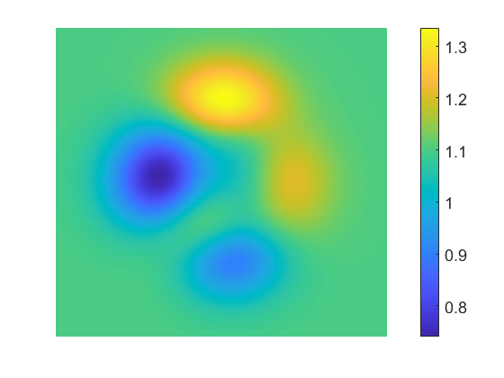
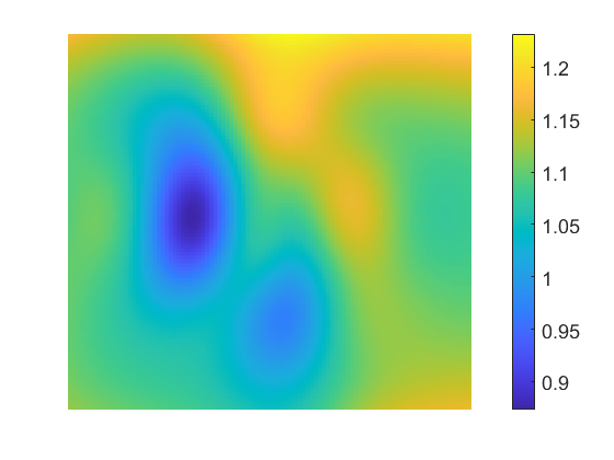
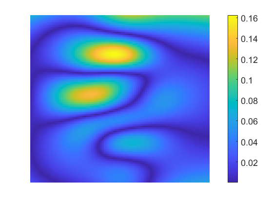
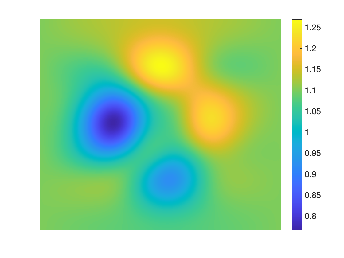
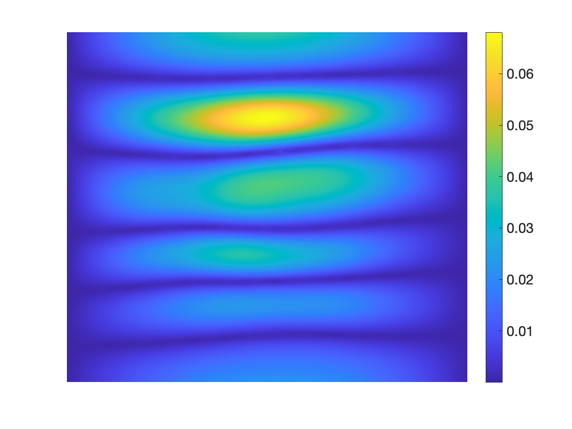
(a) $\sigma^{\dagger}$	(b) $\hat{\sigma}$	(c) $|\hat{\sigma}-\sigma^{\dagger}|$

Figure 2: The reconstructions for Example 4.1 with exact data, obtained by the neural network approach (top) and the iterative algorithm of Nachman et al. (bottom).

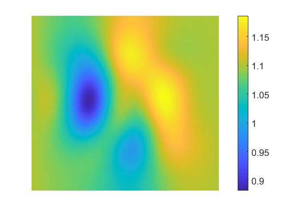
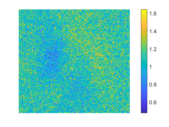
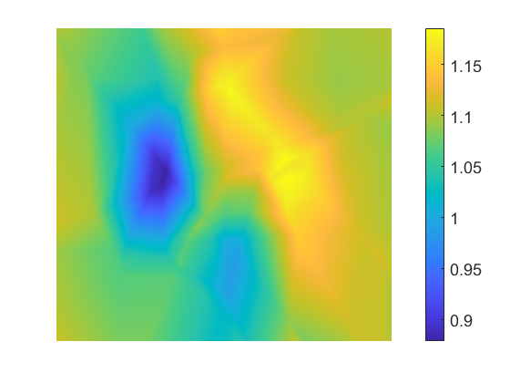
(a) $a^{\dagger}$	(b) $a^{\delta}$	(c) $\hat{a}$
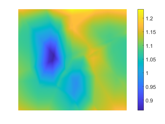
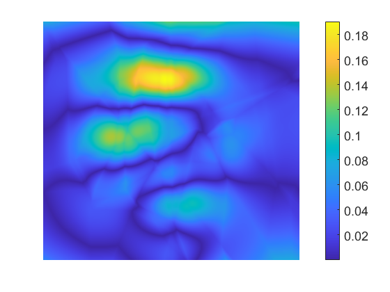
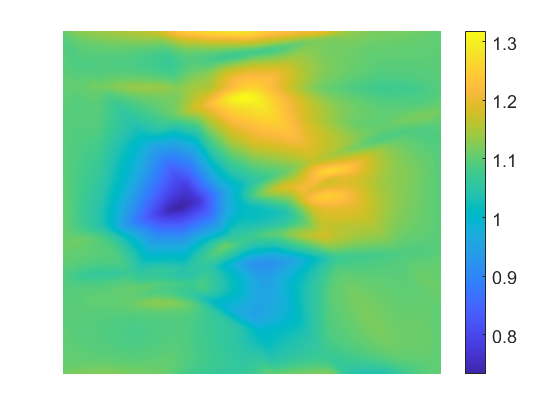
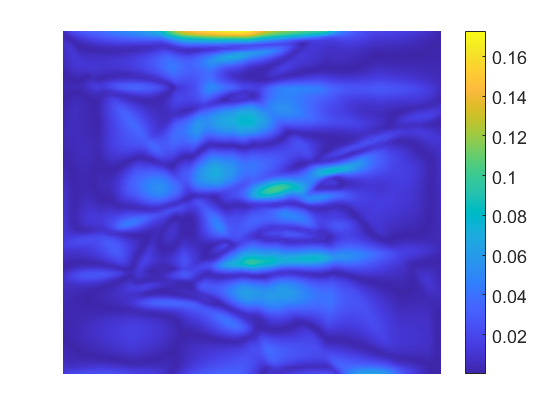
(d) $\sigma^{\dagger}$	(e) $\hat{\sigma}$	(f) $|\hat{\sigma}-\sigma^{\dagger}|$

Figure 3: Noisy data $a^{\delta}$ versus denoised data for Example 4.1 with $\delta=10\%$ noise (top), and the reconstructions by the neural network approach (middle) and the iterative algorithm at the 14th iterations (bottom).

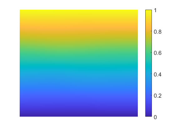
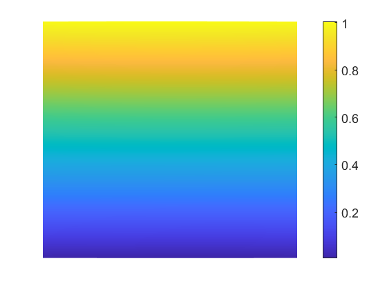
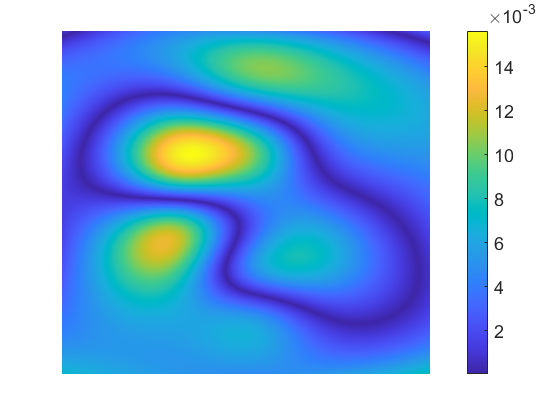
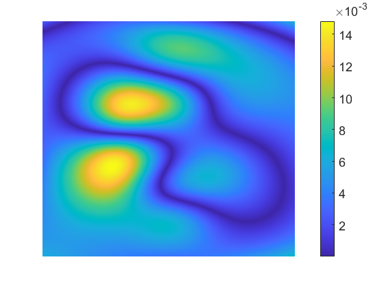
(a) $u^{\dagger}$	(b) $\hat{u}$	(c) $|\hat{u}-u^{\dagger}|$

Figure 4: The reconstructions of $u$ for Example 4.1 with exact data (top) and with data with $\delta=10\%$ noise (bottom), obtained by the neural network approach.

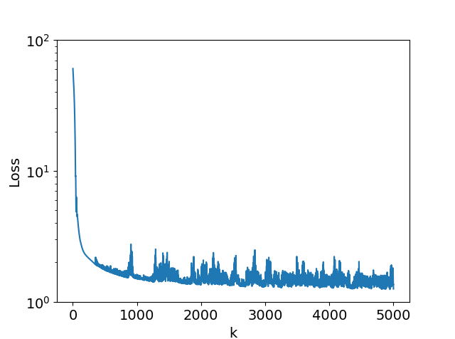
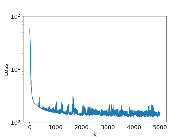
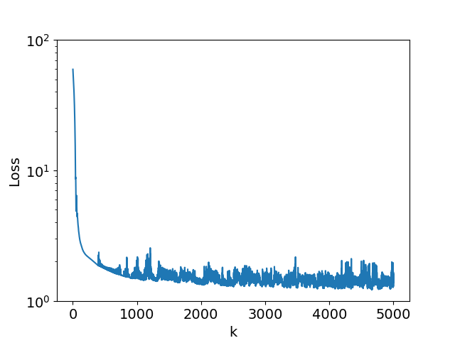
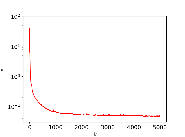
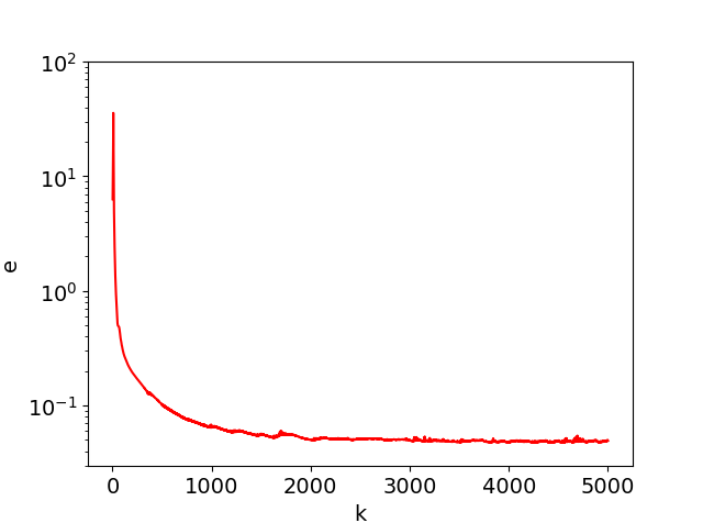
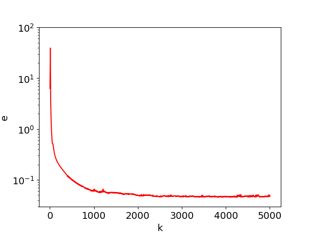
(a) $\delta=0\%$	(b) $\delta=1\%$	(c) $\delta=10\%$

Figure 5: The convergence of the empirical loss and the $L^{2}$-relative error $e(\hat{\sigma})$ versus training epoch $k$ for Example 4.1 at various noise levels.

First we show the reconstruction performance. Fig. 2 shows the recovered conductivity $\hat{\sigma}$ for exact data and the error $|\hat{\sigma}-\sigma^{\dagger}|$, along with the results by the iterative approach (cf. Section 2). The error plots show that the neural network approximation has largest error in regions near the top-bottom edges, and that the attainable accuracy is inferior to that by the iterative algorithm (which can be made arbitrarily accurate for exact data, since the algorithm converges to the exact conductivity $\sigma^{\dagger}$ [54]). This accuracy limitation is attributed to the optimization error; see the discussions below. For the data with $10\%$ noise, denoising using neural networks is quite effective in recovering the current density magnitude $a$, cf. Fig. 3, concurring with the empirical success for deep image prior [68]. It is worth noting that for noisy data $a^{\delta}$, denoising alone is insufficient to ensure the convergence of the iterative algorithm, which is only guaranteed for admissible data pairs. Thus the iterative algorithm requires careful early stopping, in order to obtain the best possible reconstruction, and a few extra iterations can greatly deteriorate the reconstruction quality. To the best of our knowledge, a provable stopping rule for the algorithm is still unavailable. Hence, in the numerical experiments, we have chosen the optimal iteration index so that the error is smallest. In the proposed approach, the neural network learns the direct solution $u$ from noisy $a^{\delta}$, and it is observed to be very robust with respect to the presence of noise, cf. Fig. 4. More surprisingly, the approach seems to be fairly stable in the iteration index, cf. Fig. 5 below, and additional iterations do not lead to much deteriorated reconstructions, despite the fact that the employed neural network has high expressivity for approximating rather irregular functions and thus in principle might be susceptible to severe over-fitting.

In the neural network approach, there are various problem / algorithmic parameters influencing the overall performance, e.g., number of training points ($n_{1}$ and $n_{2}$), network parameters (width, depth, and activation function) and noise level $\delta$. However, a comprehensive guidance for properly choosing these parameters suitably is still completely missing. Instead, we explore the issue empirically. Tables 1 and 6(a) show the relative $L^{2}$-error of the recovered voltage $\hat{u}$ and conductivity $\hat{\sigma}$, respectively, at different noise levels and different $n_{1}$. The algorithm is observed to be very robust with respect to the presence of data noise, and the reconstruction remains fairly accurate even for up to 10% data noise. This contrasts sharply with more traditional optimization based approaches. However, there is also an accuracy limitation of the approach, i.e., the reconstruction cannot be made arbitrarily accurate for exact data $a^{\dagger}$. This is attributed to the optimization error, which has also been observed across a broad range of solvers based on neural networks [58, 22]. Tables 6(b)-6(d) show that the error $e(\hat{\sigma})$ of the recovered conductivity $\hat{\sigma}$ does not vary much with various parameters, e.g., different network architectures. This agrees with the convergence behavior of the optimization algorithm in Fig. 5: it is largely independent of the noise level $\delta$, and the value of the loss eventually stagnates at a certain level, so is for the reconstruction error $e(\hat{\sigma})$. Thus, the optimization error seems dominating when the noise level $\delta$ is low. In particular, further iterations do not affect much the accuracy of the reconstructions. Although not presented, a similar convergence behavior is also observed for much larger neural networks. Of course, if the neural network is vastly expressive and the optimization algorithm continues running for many iterations, it is expected and also numerically observed that over-fitting eventually will kick in, due to the lack of explicit regularization, necessitating the use of early stopping or explicit regularization then. These studies show the typical behavior of neural network based approaches, i.e., high-robustness to the data noise and the low sensitivity to the stopping iteration index.

Last we briefly comment on the computational expense. Due to the high non-convexity of the empirical loss $\widehat{\mathcal{L}}_{\gamma}(\theta)$ (in $\theta$), a global optimizer is often challenging to obtain. The stand-alone optimizers, e.g., ADAM / L-BFGS, often take hundreds of iterations to reach convergence, cf. Fig. 5. Thus, overall the neural network approach appears less efficient than the iterative algorithm when the direct problem is solved using the standard Galerkin finite element method, for which there are highly customized and thus very efficient linear solvers. One important issue is to accelerate the neural network approach.

Table 1: The $L^{2}$-relative error of the recovered $u$ v.s. $\delta$ and $n_{1}$.

$n_{1}\backslash\delta$	0%	1%	10%
4000	1.73e-2	9.98e-3	1.06e-2
6000	9.57e-3	1.50e-2	1.02e-2
8000	9.95e-3	9.95e-3	9.83e-3
10000	1.23e-2	1.51e-2	9.50e-3

Table 2: The variation of the relative $L^{2}$ error $e(\hat{\sigma})$ with respect to various parameters.

$n_{1}\backslash\delta$	0%	1%	10%
4000	4.83e-2	4.79e-2	4.80e-2
6000	4.82e-2	5.06e-2	4.70e-2
8000	4.89e-2	4.82e-2	4.75e-2
10000	4.68e-2	4.91e-2	4.70e-2

(a) $e$ v.s. $n_{1}$ and $\delta$

$\gamma\backslash\zeta$	0.01	0.1	1
10	4.99e-2	5.06e-2	4.71e-2
100	4.70e-2	4.81e-2	4.79e-2
1000	4.79e-2	4.79e-2	4.87e-2
10000	4.79e-2	4.79e-2	4.92e-2

(b) $e$ v.s. $\gamma$ and $\zeta$

$L\backslash\mathcal{W}$	10	20	40
2	4.17e-2	4.17e-2	4.20e-2
4	4.31e-2	4.08e-2	4.26e-2
6	4.67e-2	4.14e-2	4.30e-2
9	4.70e-2	4.50e-2	4.73e-2

(c) $e$ v.s. $L$ and $\mathcal{W}$

$n_{2}\backslash n_{1}$	4000	6000	8000	10000
40	8.11e-2	9.04e-2	6.96e-2	7.21e-2
400	4.79e-2	4.75e-2	5.06e-2	4.81e-2
1000	4.66e-2	4.57e-2	4.88e-2	4.70e-2
4000	4.69e-2	4.64e-2	4.63e-2	4.78e-2

(d) $e$ v.s. $n_{1}$ and $n_{2}$

The second example is concerned with recovering a discontinuous conductivity $\sigma^{\dagger}$.

Example 4.2.

The exact conductivity $\sigma^{\dagger}$ is $\sigma^{\dagger}(x,y)=1+\chi_{\{x>0.5\}}e^{-2((x-0.5)^{2}+(y-0.5)^{2})},$ where $\chi_{S}$ denotes the characteristic function of the set $S$.

We present reconstructions for the data with $10\%$ noise. The results by the neural network approach and the iterative one in Fig. 6 indicate that the reconstructions by the two algorithms are of very similar qualities. The error plots indicate that for both approaches, the error is mainly along the discontinuous interface. Quantitatively, the relative $L^{2}$ error of the conductivity by the neural network approach is 3.68e-2, which is of almost no difference when compared to that for the noiseless case (3.99e-2). This clearly shows the remarkable robustness of the approach for noisy data. These observations fully agree with that for the recovery of the voltage $u$ for exact and noisy data in Fig. 7: visually there is no difference between the two cases.

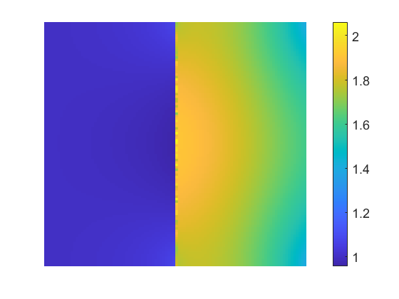
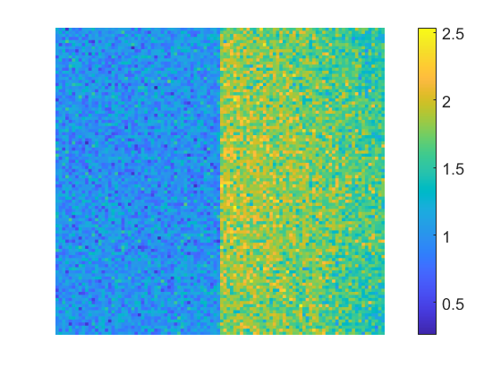
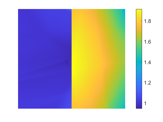
(a) $a^{\dagger}$	(b) $a^{\delta}$	(c) $\hat{a}$
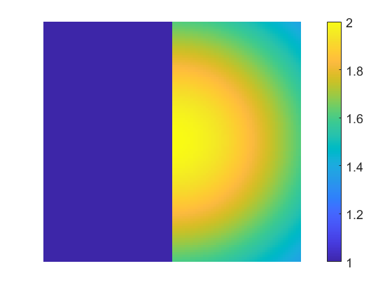
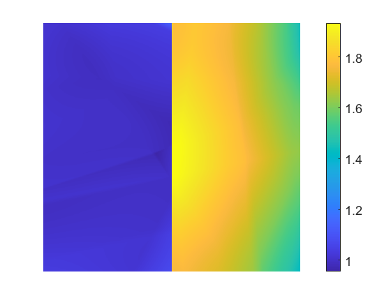
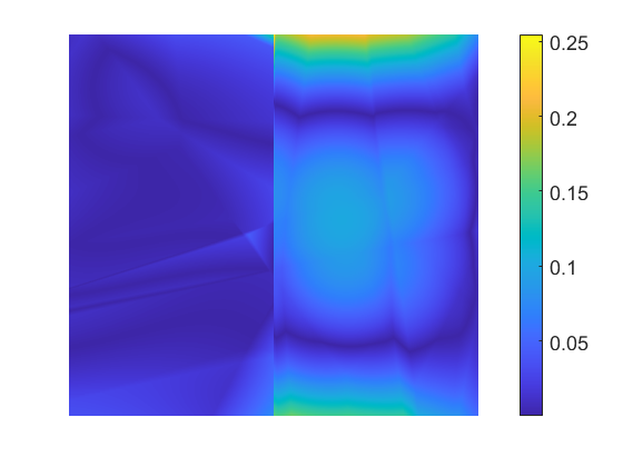
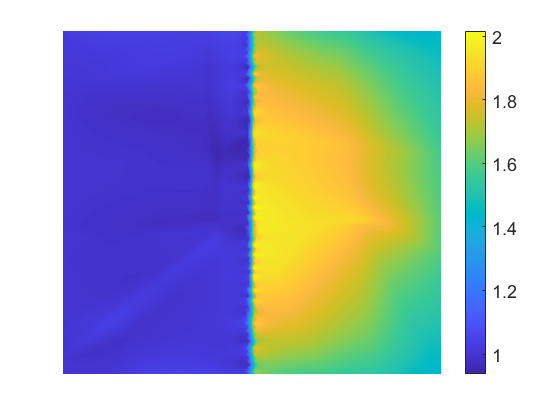
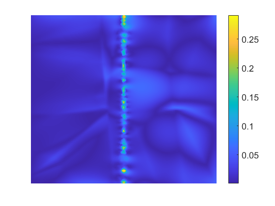
(d) $\sigma^{\dagger}$	(e) $\hat{\sigma}$	(f) $|\hat{\sigma}-\sigma^{\dagger}|$

Figure 6: Noisy data $a^{\delta}$ versus denoised data for Example 4.2 with $\delta=10\%$ noise (top), and the reconstructions obtained by the neural network (middle) and the iterative algorithm (bottom) at 6 iterations.

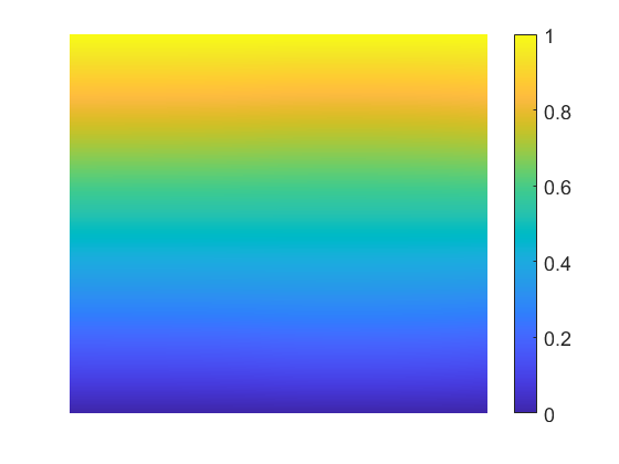
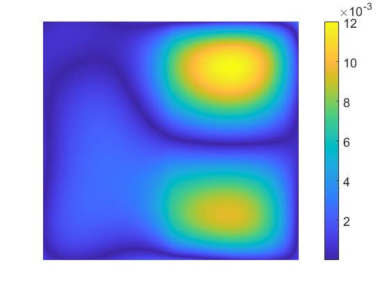
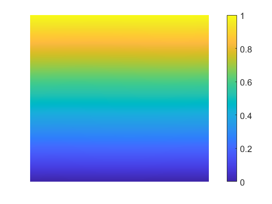
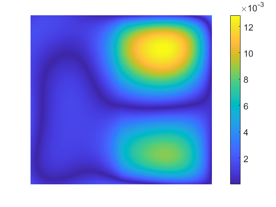
(a) $u^{\dagger}$	(b) $\hat{u}$	(c) $|\hat{u}-u^{\dagger}|$

Figure 7: The reconstructions of $u$ for Example 4.2 without (top) and with (bottom) $\delta=10\%$ noise in the data, obtained by the neural network approach.

The last example is concerned with recovering the Shepp-Logan CT phantom.

Example 4.3.

In this example, the exact conductivity $\sigma^{\dagger}$ is a piecewise constant function corresponding to the standard Shepp-Logan CT image. The intensity of the image is rescaled to a conductivity distribution $\sigma$ ranging from 1 to 1.8 S/m.

In this example, for the reconstruction of $\sigma$, we consider 1$\%$ noise, since the current density magnitude $a$ is highly challenging for denoising, due to the low contrast of conductivity in different regions (within the range from 1 to 1.8). The reconstructions of the conductivity for data with $1\%$ noise in Fig. 8 is nearly identical with that for exact data (which is not shown). It only tends to be less accurate near the top-bottom edges of the outer circle, where the exact conductivity $\sigma^{\dagger}$ undergoes big sudden jumps. This observation agrees with the previous examples. Nevertheless, the learning of the neural network at step (i) of the algorithm (cf. section 2.2) is not affected much by high noise levels: even for up to 10% noise, the recovered voltage $u$ remains highly accurate, cf. Fig. 9, confirming the remarkable robustness of the neural network approach with respect to data noise.

Last, we examine the case of partial interior data, i.e. with $a$ on a subdomain $\Omega^{\prime}\subset\Omega$. Then the population loss $\mathcal{L}_{\gamma}^{\prime}(u)$ is given by

$$\mathcal{L}_{\gamma}^{\prime}(u)=\int_{\Omega^{\prime}}a|Du|+\gamma\int_{\partial\Omega}a|u-g|\mathrm{d}s$$

This functional is then discretized by neural networks, but with random sampling points in the subdomain $\Omega^{\prime}$. In this case, we reconstruct only the conductivity distributions inside $\Omega^{\prime}$. In the experiment, we take $\Omega^{\prime}$ to be a square region inside the outer circle. The reconstructions for data with $1\%$ noise in Fig. 8 show that the network can accurately recover the conductivity values from partial data apart from the regions near the outer circle. This shows the feasibility of the approach for partial data, corroborating existing theoretical results [49]. Interestingly, even with $10\%$ noise in the data, the recovery of $u$ remains very accurate, cf. Fig. 9, which again shows the robustness of the approach with respect to data noise.

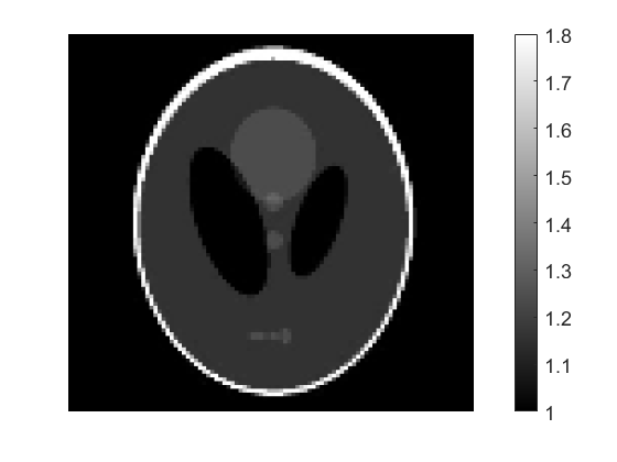
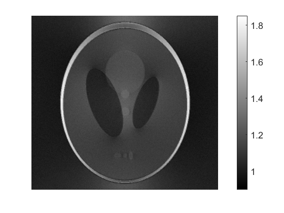
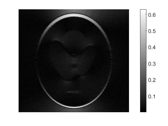
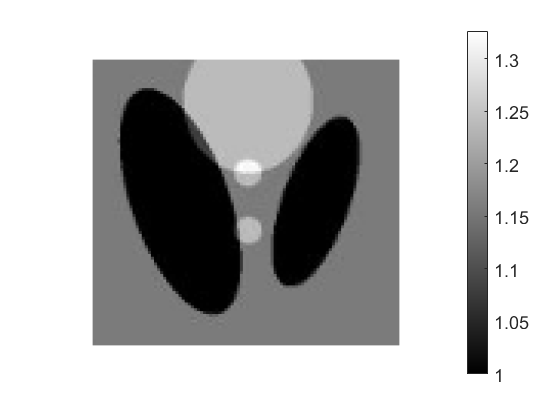
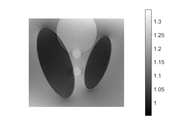
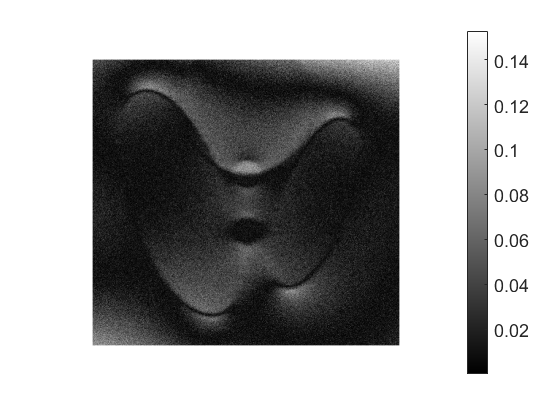
(a) $\sigma^{\dagger}$	(b) $\hat{\sigma}$	(c) $|\hat{\sigma}-\sigma^{\dagger}|$

Figure 8: The reconstructions for Example 4.3 for full data (top) and partial data with 1% noise.

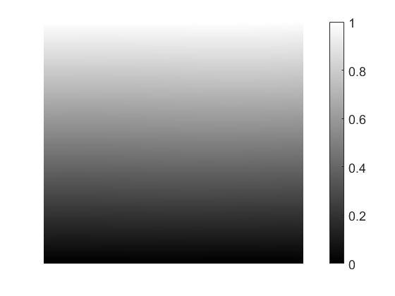
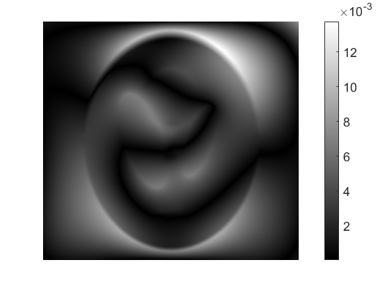
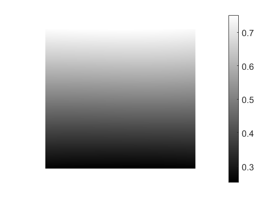
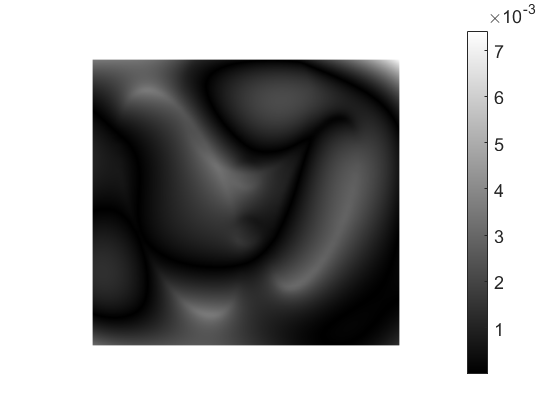
(a) $u^{\dagger}$	(b) $\hat{u}$	(c) $|\hat{u}-u^{\dagger}|$

Figure 9: The reconstructions of $u$ for Example 4.3 for full data (top) and partial data (bottom), with $\delta=10\%$ noise.

5 Conclusion

In this work we have developed a direct and novel neural network based reconstruction technique for imaging the conductivity distribution from the magnitude of the internal current density. The reconstruction problem was formulated as a relaxed weighted least-gradient problem, whose minimizer was then approximated by standard fully connected feedforward neural networks. We have also provided a preliminary analysis for the convergence rate of the generalization error, which provides guidelines for properly choosing the depth, width, total number of parameters of neural networks, and the number of training points in order to achieve the desired convergence rate. The performance and distinct features of the proposed approach were illustrated on a wide range of numerical experiments.

The excellent performance of the neural network based algorithm motivates further research, for which there are several interesting directions. First, the numerical findings suggest that the neural network reconstruction is highly robust with respect to noise. This is commonly attributed to the implicit bias induced by the neural network architecture (e.g., deep image prior [68]) as well as the optimizer. However, the precise characterization of the implicit bias within the context or the mechanism behind the robustness remains mysterious. Second, the relative approximation errors for the neural network reconstructed conductivities are usually only of order $10^{-2}$, even for relatively large neural networks. This appears to be suboptimal, in view of the approximation capacity of deep neural networks. The experiments indicate that the source of error might be attributed to the optimization aspect: the optimizer may have only found a local minimizer due to the complex landscape, and may be unable to reach a global optimizer. Then one natural question is how to achieve better approximation by choosing optimization algorithms different from stand-alone optimizers, e.g., L-BFGS, SGD and Adam. Note that these algorithms often take many iterations to reach convergence, and acceleration strategies are highly desired for better computational efficiency. Third, it is interesting to extend the convergence analysis to related models, e.g., complete electrode model for CDII or other imaging modalities with variational formulations. Fourth and last, one highly acclaimed feature of approaches based on deep neural networks is that they may hold significant potentials to overcome the notorious curse of dimensionality when the solution satisfies certain favorable properties, e.g., lying in Barron space [43]. It is thus of much interest to extend the analysis and numerics to the high-dimensional setting.

References

- [1] B. J. Adesokan, B. Jensen, B. Jin, and K. Knudsen. Acousto-electric tomography with total variation regularization. Inverse Problems, 35(3):035008, 25, 2019.
- [2] H. Ammari. An Introduction to Mathematics of Emerging Biomedical Imaging. Springer, Berlin, 2008.
- [3] M. Anthony and P. L. Bartlett. Neural Network Learning: Theoretical Foundations. Cambridge University Press, Cambridge, 1999.
- [4] I. Babuška. The finite element method with penalty. Math. Comp., 27:221–228, 1973.
- [5] G. Bal. Hybrid inverse problems and internal functionals. In Inverse problems and applications: inside out. II, pages 325–368. Cambridge Univ. Press, Cambridge, 2013.
- [6] G. Bao, X. Ye, Y. Zang, and H. Zhou. Numerical solution of inverse problems by weak adversarial networks. Inverse Problems, 36(11):115003, 31, 2020.
- [7] L. Bar and N. Sochen. Strong solutions for PDE-based tomography by unsupervised learning. SIAM J. Imaging Sci., 14(1):128–155, 2021.
- [8] P. L. Bartlett, D. J. Foster, and M. Telgarsky. Spectrally-normalized margin bounds for neural networks. In 31st Conference on on Advances in Neural Information Systems, pages 6240–6249, 2017.
- [9] P. L. Bartlett, N. Harvey, C. Liaw, and A. Mehrabian. Nearly-tight VC-dimension and pseudodimension bounds for piecewise linear neural networks. J. Mach. Learn. Res., 20:Paper No. 63, 17, 2019.
- [10] P. L. Bartlett and S. Mendelson. Rademacher and Gaussian complexities: risk bounds and structural results. J. Mach. Learn. Res., 3:463–482, 2002.
- [11] A. G. Baydin, B. A. Pearlmutter, A. A. Radul, and J. M. Siskind. Automatic differentiation in machine learning: a survey. J. Mach. Learn. Res., 18:Paper No. 153, 43, 2017.
- [12] J. Berner, P. Grohs, and A. Jentzen. Analysis of the generalization error: empirical risk minimization over deep artificial neural networks overcomes the curse of dimensionality in the numerical approximation of Black-Scholes partial differential equations. SIAM J. Math. Data Sci., 2(3):631–657, 2020.
- [13] L. Borcea. Electrical impedance tomography. Inverse Problems, 18(6):R99–R136, 2002.
- [14] L. Bottou, F. E. Curtis, and J. Nocedal. Optimization methods for large-scale machine learning. SIAM Rev., 60(2):223–311, 2018.
- [15] R. H. Byrd, P. Lu, J. Nocedal, and C. Y. Zhu. A limited memory algorithm for bound constrained optimization. SIAM J. Sci. Comput., 16(5):1190–1208, 1995.
- [16] V. Caselles, G. Facciolo, and E. Meinhardt. Anisotropic Cheeger sets and applications. SIAM J. Imaging Sci., 2(4):1211–1254, 2009.
- [17] F. Cucker and S. Smale. On the mathematical foundations of learning. Bull. Amer. Math. Soc. (N.S.), 39(1):1–49, 2002.
- [18] M. Dissanayake and N. Phan-Thien. Neural-network based approximations for solving partial differential equations. Comm. Numer. Methods Engrg., 10:195–201, 1994.
- [19] C. Duan, Y. Jiao, Y. Lai, D. Li, X. Lu, and Z. Y. Jerry. Convergence rate analysis for deep Ritz method. Commun. Comput. Phys., 31(4):1020–1048, 2022.
- [20] R. M. Dudley. The sizes of compact subsets of Hilbert space and continuity of Gaussian processes. J. Functional Analysis, 1(3):290–330, 1967.
- [21] W. E, J. Han, and A. Jentzen. Algorithms for solving high dimensional PDEs: from nonlinear Monte Carlo to machine learning. Nonlinearity, 35(1):278–310, 2022.
- [22] W. E and B. Yu. The deep Ritz method: a deep learning-based numerical algorithm for solving variational problems. Commun. Math. Stat., 6(1):1–12, 2018.
- [23] L. C. Evans and R. F. Gariepy. Measure Theory and Fine Properties of Functions. Textbooks in Mathematics. CRC Press, Boca Raton, FL, revised edition, 2015.
- [24] K. R. Foster and H. P. Schwan. Dielectric properties of tissues and biological materials: a critical review. Crit. Rev. Biomed. Eng., 17(1):25–104, 1989.
- [25] H. R. Gamba, R. Bayford, and D. Holder. Measurement of electrical current density distribution in a simple head phantom with magnetic resonance imaging. Phys. Med. Biol., 44(1):281–91, 1999.
- [26] I. Gühring and M. Raslan. Approximation rates for neural networks with encodable weights in smoothness spaces. Neural Networks, 134:107–130, 2021.
- [27] R. Guo and J. Jiang. Construct deep neural networks based on direct sampling methods for solving electrical impedance tomography. SIAM J. Sci. Comput., 43(3):B678–B711, 2021.
- [28] N. Hoell, A. Moradifam, and A. Nachman. Current density impedance imaging of an anisotropic conductivity in a known conformal class. SIAM J. Math. Anal., 46(3):1820–1842, 2014.
- [29] K. Hoffmann and K. Knudsen. Iterative reconstruction methods for hybrid inverse problems in impedance tomography. Sens. Imaging, 15:96, 27 pp., 2014.
- [30] Q. Hong, J. W. Siegel, and J. Xu. A priori analysis of stable neural network solutions to numerical PDEs. Preprint, arXiv:2104.02903, 2021.
- [31] Y. Ider and L. Muftuler. Measurement of AC magnetic field distribution using magnetic resonance imaging. IEEE Trans. Med. Imaging, 16:617–622, 1997.
- [32] K. Ito and B. Jin. Inverse Problems: Tikhonov Theory and Algorithms. World Scientific Publishing Co. Pte. Ltd., Hackensack, NJ, 2015.
- [33] R. L. Jerrard, A. Moradifam, and A. I. Nachman. Existence and uniqueness of minimizers of general least gradient problems. J. Reine Angew. Math., 734:71–97, 2018.
- [34] Y. Jiao, Y. Lai, Y. Lou, Y. Wang, and Y. Yang. Error analysis of deep Ritz methods for elliptic equations. Preprint, arXiv:2107.14478, 2021.
- [35] M. Johannes and M. Zeinhofer. Error estimates for the variational training of neural networks with boundary penalty. Preprint, arXiv:2103.01007, 2021.
- [36] M. L. Joy, G. C. Scott, and M. Henkelman. In vivo detection of applied electric currents by magnetic resonance imaging. Magnet. Resonance Imaging, 7(1):89–94, 1989.
- [37] Y. Khoo and L. Ying. SwitchNet: a neural network model for forward and inverse scattering problems. SIAM J. Sci. Comput., 41(5):A3182–A3201, 2019.
- [38] S. Kim, O. Kwon, J. K. Seo, and J.-R. Yoon. On a nonlinear partial differential equation arising in magnetic resonance electrical impedance tomography. SIAM J. Math. Anal., 34(3):511–526, 2002.
- [39] D. P. Kingma and J. Ba. Adam: A method for stochastic optimization. In 3rd International Conference for Learning Representations, San Diego, 2015, 2015.
- [40] I. E. Lagaris, A. Likas, and D. I. Fotiadis. Artificial neural networks for solving ordinary and partial differential equations. IEEE Trans. Neural Networks, 9(5):987–1000, 1998.
- [41] H. Liu, B. Jin, and X. Lu. Imaging anisotropic conductivities from current densities. SIAM J. Imag. Sci., pages in press, arXiv:2203.02164, 2022.
- [42] R. Lopez and A. Moradifam. Stability of current density impedance imaging. SIAM J. Math. Anal., 52(5):4506–4523, 2020.
- [43] Y. Lu, J. Lu, and M. Wang. A priori generalization analysis of the deep ritz method for solving high dimensional elliptic partial differential equations. In Conference on Learning Theory, pages 3196–3241. PMLR, 2021.
- [44] T. Luo and H. Yang. Two-layer neural networks for partial differential equations: Optimization and generalization theory. Preprint, arXiv:2006.15733, 2020.
- [45] J. M. Mazón. The Euler-Lagrange equation for the anisotropic least gradient problem. Nonlinear Anal. Real World Appl., 31:452–472, 2016.
- [46] S. Mendelson. A few notes on statistical learning theory. In S. Mendelson and A. J. Smola, editors, Advanced Lectures on Machine Learning, pages 1–40. Springer-Verlag, Berlin, 2003.
- [47] J. S. Moll. The anisotropic total variation flow. Math. Ann., 332(1):177–218, 2005.
- [48] C. Montalto and P. Stefanov. Stability of coupled-physics inverse problems with one internal measurement. Inverse Problems, 29(12):125004, 2013.
- [49] C. Montalto and A. Tamasan. Stability in conductivity imaging from partial measurements of one interior current. Inverse Probl. Imaging, 11(2):339–353, 2017.
- [50] A. Moradifam, A. Nachman, and A. Tamasan. Uniqueness of minimizers of weighted least gradient problems arising in hybrid inverse problems. Calc. Var. Partial Differential Equations, 57(1):Paper No. 6, 14, 2018.
- [51] A. Moradifam, A. Nachman, and A. Timonov. A convergent algorithm for the hybrid problem of reconstructing conductivity from minimal interior data. Inverse Problems, 28(8):084003, 23, 2012.
- [52] T. Morimoto, S. Kimura, Y. Konishi, K. Komaki, T. Uyama, Y. Monden, D. Y. Kinouchi, and D. T. Iritani. A study of the electrical bio-impedance of tumors. Invest. Surg., 6(1):25–32, 1993.
- [53] A. Nachman, A. Tamasan, and A. Timonov. Conductivity imaging with a single measurement of boundary and interior data. Inverse Problems, 23(6):2551–2563, 2007.
- [54] A. Nachman, A. Tamasan, and A. Timonov. Recovering the conductivity from a single measurement of interior data. Inverse Problems, 25(3):035014, 16, 2009.
- [55] A. Nachman, A. Tamasan, and J. Veras. A weighted minimum gradient problem with complete electrode model boundary conditions for conductivity imaging. SIAM J. Appl. Math., 76(4):1321–1343, 2016.
- [56] M. Z. Nashed and A. Tamasan. Structural stability in a minimization problem and applications to conductivity imaging. Inverse Probl. Imaging, 5(1):219–236, 2011.
- [57] S. Pakravan, P. A. Mistani, M. A. Aragon-Calvo, and F. Gibou. Solving inverse-PDE problems with physics-aware neural networks. J. Comput. Phys., 440:Paper No. 110414, 31, 2021.
- [58] M. Raissi, P. Perdikaris, and G. E. Karniadakis. Physics-informed neural networks: a deep learning framework for solving forward and inverse problems involving nonlinear partial differential equations. J. Comput. Phys., 378:686–707, 2019.
- [59] H. Robbins and S. Monro. A stochastic approximation method. Ann. Math. Statistics, 22(3):400–407, 1951.
- [60] N. Schreuder. Bounding the expectation of the supremum of empirical processes indexed by Hölder classes. Math. Methods Statist., 29(1):76–86, 2020.
- [61] G. C. Scott, M. L. G. Joy, R. L. Armstrong, and R. M. Henkelman. Measurement of nonuniform current density by magnetic resonance. IEEE Trans. Med. Imag., 10:362–374, 1991.
- [62] J. K. Seo, K. C. Kim, A. Jargal, K. Lee, and B. Harrach. A learning-based method for solving ill-posed nonlinear inverse problems: a simulation study of lung EIT. SIAM J. Imaging Sci., 12(3):1275–1295, 2019.
- [63] S. Shalev-Shwartz and S. Ben-David. Understanding Machine Learning: From Theory to Algorithms. Cambridge University Press, 2014.
- [64] J. Sirignano and K. Spiliopoulos. DGM: a deep learning algorithm for solving partial differential equations. J. Comput. Phys., 375:1339–1364, 2018.
- [65] N. Srebro, K. Sridharan, and A. Tewari. Smoothness, low noise and fast rates. In Advances in Neural Information Processing Systems, pages 2199–2207, 2010.
- [66] A. Tamasan and A. Timonov. A regularized weighted least gradient problem for conductivity imaging. Inverse Problems, 35(4):045006, 20, 2019.
- [67] A. Tamasan, A. Timonov, and J. Veras. Stable reconstruction of regular 1-harmonic maps with a given trace at the boundary. Appl. Anal., 94(6):1098–1115, 2015.
- [68] D. Ulyanov, A. Vedaldi, and V. Lempitsky. Deep image prior. Int. J. Comput. Vis., 128(7):1867–1888, 2020.
- [69] S. A. van de Geer. Applications of Empirical Process Theory. Cambridge University Press, Cambridge, 2000.
- [70] T. Widlak and O. Scherzer. Hybrid tomography for conductivity imaging. Inverse Problems, 28(8):084008, 28, 2012.
- [71] J. Xu. Finite neuron method and convergence analysis. Commun. Comput. Phys., 28(5):1707–1745, 2020.
- [72] K. Xu and E. Darve. Physics constrained learning for data-driven inverse modeling from sparse observations. J. Comput. Phys., 453:Paper No. 110938, 24, 2022.
- [73] H. Yazdanian and K. Knudsen. Numerical conductivity reconstruction from partial interior current density information in three dimensions. Inverse Problems, 37(10):Paper No. 105010, 26, 2021.