OccamNets: Mitigating Dataset Bias by Favoring Simpler Hypotheses

Abstract

Dataset bias and spurious correlations can significantly impair generalization in deep neural networks. Many prior efforts have addressed this problem using either alternative loss functions or sampling strategies that focus on rare patterns. We propose a new direction: modifying the network architecture to impose inductive biases that make the network robust to dataset bias. Specifically, we propose OccamNets, which are biased to favor simpler solutions by design. OccamNets have two inductive biases. First, they are biased to use as little network depth as needed for an individual example. Second, they are biased toward using fewer image locations for prediction. While OccamNets are biased toward simpler hypotheses, they can learn more complex hypotheses if necessary. In experiments, OccamNets outperform or rival state-of-the-art methods run on architectures that do not incorporate these inductive biases. Furthermore, we demonstrate that when the state-of-the-art debiasing methods are combined with OccamNets results further improve.

1 Introduction

Frustra fit per plura quod potest fieri per pauciora

William of Occam, Summa Totius Logicae (1323 CE)

Spurious correlations and dataset bias greatly impair generalization in deep neural networks [2, 6, 23, 62]. This problem has been heavily studied. The most common approaches are re-sampling strategies [8, 15, 22, 57], altering optimization to mitigate bias [55], adversarial unlearning [1, 20, 53, 77], learning invariant representations [5, 11, 67], and ensembling with bias-amplified models [7, 12, 47]. Here, we propose a new approach: incorporating architectural inductive biases that combat dataset bias.

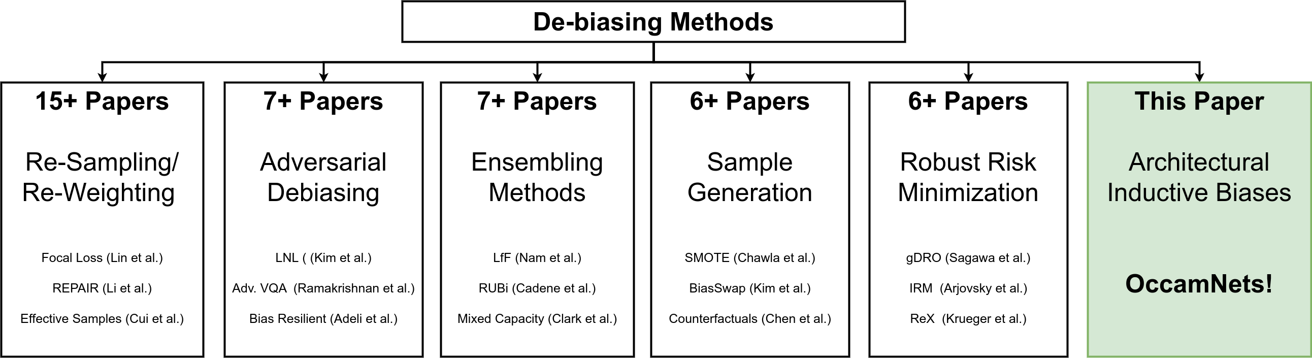
Figure 1: OccamNets focus on architectural inductive biases, which is an orthogonal direction to tackling dataset biases compared to the existing works.

In a typical feedforward network, each layer can be considered as computing a function of the previous layer, with each additional layer making the hypothesis more complex. Given a system trained to predict multiple categories, with some being highly biased, this means the network uses the same level of complexity across all of the examples, even when some examples should be classified with simpler hypotheses (e.g., less depth). Likewise, pooling in networks is typically uniform in nature, so every location is used for prediction, rather than only the minimum amount of information. In other words, typical networks violate Occam’s razor. Consider the Biased MNIST dataset [62], where the task is to recognize a digit while remaining invariant to multiple spuriously correlated factors, which include colors, textures, and contextual biases. The most complex hypothesis would exploit every factor during classification, including the digit’s color, texture, or background context. A simple hypothesis would instead be to focus on the digit’s shape and to ignore these spuriously correlated factors that work very well during training but do not generalize. We argue that a network should be capable of adapting its hypothesis space for each example, rather than always resorting to the most complex hypothesis, which would help it to ignore extraneous variables that hinder generalization.

Here, we propose convolutional OccamNets which have architectural inductive biases that favor using the minimal amount of network depth and the minimal number of image locations during inference for a given example. The first inductive bias is implemented using early exiting, which has been previously studied for speeding up inference. The network is trained such that later layers focus on examples earlier layers find hard, with a bias toward exiting early. The second inductive bias replaces global average pooling before a classification layer with a function that is regularized to favor pooling with fewer image locations from class activation maps (CAMs). We hypothesize this would be especially useful for combating background and contextual biases [3, 63]. OccamNets are complementary to existing approaches and can be combined with them.

In this paper, we demonstrate that architectural inductive biases are effective at mitigating dataset bias. Our specific contributions are:

• We introduce the OccamNet architecture, which has architectural inductive biases for favoring simpler solutions to help overcome dataset biases. OccamNets do not require the biases to be explicitly specified during training, unlike many state-of-the-art debiasing algorithms.

• In experiments using biased vision datasets, we demonstrate that OccamNets greatly outperform architectures that do not use the proposed inductive biases. Moreover, we show that OccamNets outperform or rival existing debiasing methods that use conventional network architectures.

• We combine OccamNets with four recent debiasing methods, which all show improved results compared to using them with conventional architectures.

2 Related Work

Dataset Bias and Bias Mitigation. When trained with empirical risk minimization (ERM), deep networks have been shown to exploit dataset biases in the training data resulting in poor test generalization [23, 45, 62, 70]. Existing works for mitigating this problem have focused on these approaches: 1) focusing on rare data patterns through re-sampling [8, 40], 2) loss re-weighting [15, 57], 3) adversarial debiasing [20, 34], 4) model ensembling [7, 12], 5) minority/counterfactual sample generation [8, 9, 35] and 6) invariant/robust risk minimization [5, 36, 56]. Most of these methods require bias variables, e.g., sub-groups within a category, to be annotated [20, 34, 40, 57, 62]. Some recent methods have also attempted to detect and mitigate biases without these variables by training separate bias-amplified models for de-biasing the main model  [13, 47, 58, 71]. This paper is the first to explore architectural inductive biases for combating dataset bias.

Early Exit Networks. OccamNet is a multi-exit architecture designed to encourage later layers to focus on samples that earlier layers find difficult. Multi-exit networks have been studied in past work to speed up average inference time by minimizing the amount of compute needed for individual examples [10, 31, 66, 74], but their impact on bias-resilience has not been studied. In [59], a unified framework for studying early exit mechanisms was proposed, which included commonly used training paradigms [26, 38, 64, 73] and biological plausibility [46, 49, 50]. During inference, multi-exit networks choose the earliest exit based on either a learned criterion [10] or through a heuristic, e.g., exit if the confidence score is sufficiently high [19], exit if there is low entropy [66], or exit if there is agreement among multiple exits [79]. Recently, [19] proposed early exit networks for long-tailed datasets; however, they used a class-balanced loss and did not study robustness to hidden covariates, whereas, OccamNets generalize to these hidden variables without oracle bias labels during training.

Exit Modules and Spatial Maps. OccamNets are biased toward using fewer spatial locations for prediction, which we enable by using spatial activation maps [24, 44, 54]. While most recent convolutional neural networks (CNNs) use global average pooling followed by a linear classification layer [25, 29, 32], alternative pooling methods have been proposed, including spatial attention [4, 21, 30, 75] and dynamic pooling [30, 33, 37]. However, these methods have not been explored for their ability to combat bias mitigation, with existing bias mitigation methods adopting conventional architectures that use global average pooling instead. For OccamNets, each exit produces a class activation map, which is biased toward using fewer visual locations.

3 OccamNets

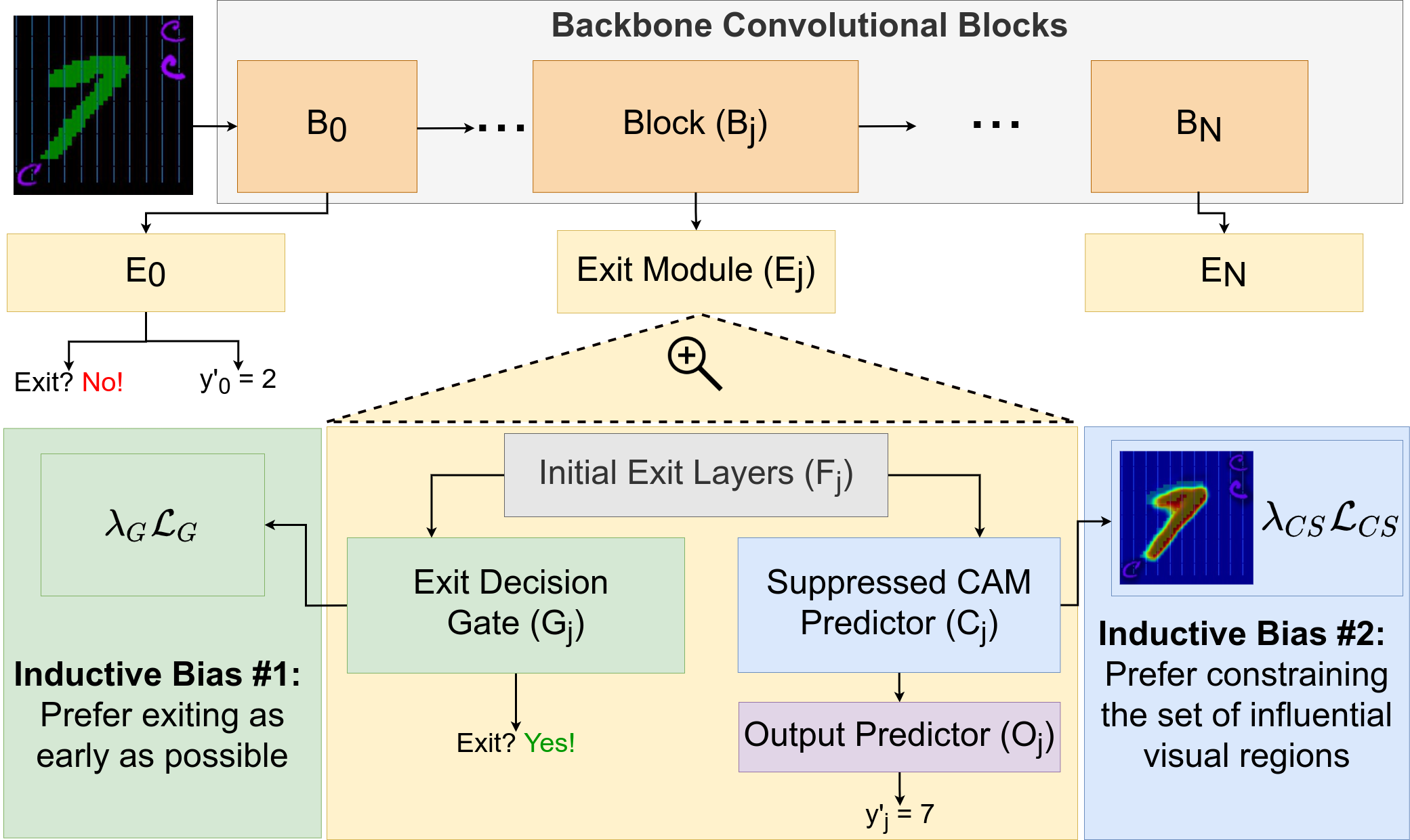
Figure 2: OccamNets are multi-exit architectures capable of exiting early through the exit decision gates. The exits yield class activation maps that are trained to use a constrained set of visual regions.

3.1 OccamNet Architecture for Image Classification

OccamNets have two inductive biases: a) they prefer exiting as early as possible, and b) they prefer using fewer visual regions for predictions. Following Occam’s principles, we implement these inductive biases using simple, intuitive ideas: early exit is based on whether or not a sample is correctly predicted during training and visual constraint is based on suppressing regions that have low confidence towards the ground truth class. We implement these ideas in a CNN. Recent CNN architectures, such as ResNets [25] and DenseNets [32], consist of multiple blocks of convolutional layers. As shown in Fig. 2, these inductive biases are enabled by attaching an exit module $E_{j}$ to block $B_{j}$ of the CNN, as the blocks serve as natural endpoints for attaching them. Below, we describe how we implement these two inductive biases in OccamNets.

In an OccamNet, each exit module $E_{j}$ takes in feature maps produced by the backbone network and processes them with $F_{j}$, which consists of two convolutional layers, producing feature maps used by the following components:

Suppressed CAM Predictors ($C_{j}$). Each $C_{j}$ consists of a single convolutional layer, taking in the feature maps from $F_{j}$ to yield class activation maps, $c$. The maps provide location wise predictions of classes. Following Occam’s principles, the usage of visual regions in these CAMs is suppressed through the CAM suppression loss $\mathcal{L}_{CS}$ described in Sec. 3.2.

Output Predictors ($O_{j}$). The output predictor applies global average pooling on the suppressed CAMs predicted by $C_{j}$ to obtain the output prediction vector, $\hat{y_{j}}\in\mathbb{R}^{n_{Y}}$, where $n_{Y}$ is the total number of classes. The entire network is trained with the output prediction loss $\mathcal{L}_{O}$, which is a weighted sum of cross entropy losses between the ground truth $y$ and the predictions $\hat{y}_{j}$ from each of the exits. Specifically, the weighting scheme is formulated to encourage the deeper layers to focus on the samples that the shallower layers find difficult. The detailed training procedure is described in Sec. 3.3.

Exit Decision Gates ($G_{j}$). During inference, OccamNet needs to decide whether or not to terminate the execution at $E_{j}$ on a per-sample basis. For this, each $E_{j}$ consists of an exit decision gate, $G_{j}$ that yields an exit decision score $g_{j}$, which is interpreted as the probability that the sample can exit from $E_{j}$. $G_{j}$ is realized via a ReLU layer followed by a sigmoid layer, taking in representations from $F_{j}$. The gates are trained via exit decision gate loss, $\mathcal{L}_{G}$ which is based on whether or not $O_{j}$ made correct predictions. The loss and the training procedure are elaborated further in Sec. 3.4.

The total loss used to train OccamNets is given by:

3.2 Training the Suppressed CAMs

To constrain the usage of visual regions, OccamNets regularize the CAMs so that only some of the cells exhibit confidence towards the ground truth class, whereas rest of the cells exhibit inconfidence i.e., have uniform prediction scores for all the classes. Specifically, let $c_{y}\in\mathbb{R}^{h\times w}$ be the CAM where each cell encodes the score for the ground truth class. Then, we apply regularization on the locations that obtain softmax scores lower than the average softmax score for the ground truth class. That is, let $\overline{c}_{y}$ be the softmax score averaged over all the cells in $c_{y}$, then the cells at location $l$, $c^{l}\in\mathbb{R}^{n_{Y}}$ are regularized if the softmax score for the ground truth class, $c^{l}_{y}$ is less than $\overline{c}_{y}$. The CAM suppression loss is:

$$\mathcal{L}_{CS}=\sum_{l=1}^{hw}\mathbbm{1}(c_{y}^{l}<\overline{c}_{y})~{}KLD(c^{l},\frac{1}{n_{Y}}\mathbf{1}),$$ (1)

where, $KLD(c^{l},\frac{1}{n_{Y}}\mathbf{1})$ is the KL-divergence loss with respect to a uniform class distribution and $\mathbbm{1}(c_{y}^{l}<\overline{c}_{y})$ ensures that the loss is applied only if the ground truth class scores lower than $\overline{c}_{y}$. The loss weight for $\mathcal{L}_{CS}$ is $\lambda_{CS}$, which is set to 0.1 for all the experiments.

3.3 Training the Output Predictors

The prediction vectors $\hat{y}$ obtained by performing global average pooling on the suppressed CAMs $c$ are used to compute the output prediction losses. Specifically, we train a bias-amplified first exit $E_{0}$, using a loss weight of: ${W}_{0}=p_{0}^{\gamma_{0}}$, where, $p_{0}$ is the softmax score for the ground truth class. Here, $\gamma_{0}>0$ encourages $E_{0}$ to amplify biases i.e., it provides higher loss weights for the samples that already have high scores for the ground truth class. This encourages $E_{0}$ to focus on the samples that it already finds easy to classify correctly. For all the experiments, we set $\gamma_{0}=3$ to sufficiently amplify the biases. The subsequent exits are then encouraged to focus on samples that the preceding exits find difficult. For this, the loss weights are defined as:

$$\mathcal{W}_{j}=(1-g_{j-1}+\epsilon),~{}\text{if j $>$ 0},$$ (2)

where, $g_{j-1}$ is the exit decision score predicted by $(j-1)^{th}$ exit decision gate and $\epsilon=0.1$ is a small offset to ensure that all the samples receive a minimal, non-zero loss weight. For the samples where $g_{j-1}$ is low, the weight loss for $j^{th}$ exit, $\mathcal{W}_{j}$ becomes high. The total output loss is then:

$$\mathcal{L}_{O}=\sum_{j=0}^{n_{E}-1}\mathcal{W}_{j}~{}CE(\hat{y}_{j},y),$$ (3)

where, $CE(\hat{y}_{j},y)$ is the cross-entropy loss and $n_{E}$ is the total number of exits. Note that $E_{j}$’s are 0-indexed and the first bias-amplified exit $E_{0}$ is not used during inference. Furthermore, during training, we prevent the gradients of $E_{0}$ from passing through $B_{0}(.)$ to avoid degrading the representations available for the deeper blocks and exits.

3.4 Training the Exit Decision Gates

Each exit decision gate $G_{j}(.)$ yields an exit probability score $\hat{g_{j}}=G_{j}(.)$. During inference, samples with $\hat{g_{j}}\geq 0.5$ exit from $E_{j}$ and samples with $\hat{g}_{j}<0.5$ continue to the next block $B_{j+1}$, if available. During training, all the samples use the entire network depth and $g_{j}$ is used to weigh losses as described in Sec. 3.3. Now, we specify the exit decision gate loss used to train $G_{j}$:

$$\mathcal{L}_{G}=\sum_{k\in\{0,1\}}\frac{\mathbbm{1}(g_{j}=k)BCE(g_{j},\hat{g_{j}})}{\sqrt{\sum\mathbbm{1}(g_{j}=k)}},$$ (4)

where $g_{j}$ is the ground truth value for the $j^{th}$ gate, which is set to $1$ if the predicted class $y^{\prime}$ is the same as the ground truth class $y$ and 0 otherwise. That is, $G_{j}$ is trained to exit if the sample is correctly predicted at depth $j$, else it is trained to continue onto the next block. Furthermore, the denominator: $\sqrt{\sum\mathbbm{1}(g_{j}=k)}$ balances out the contributions from the samples with $g=1$ and $g=0$ to avoid biasing one decision over the other. With this setup, sufficiently parameterized models that obtain $100\%$ training accuracy will result in a trivial solution where $g_{j}$ is always set to $1$ i.e., the exit will learn that all the samples can exit. To avoid this issue, we stop computing $g_{j}$ once $E_{j}$’s mean-per-class training accuracy reaches a predefined threshold $\tau_{acc,j}$. During training, we stop the gradients from $G$ from passing through $F_{j}(.)$ and $B(.)$, since this improved the training stability and overall accuracy in the preliminary experiments. The loss weight $\lambda_{G}$ is set to 1 in all the experiments.

4 Experimental Setup

4.1 Datasets

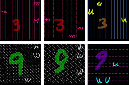
(a) Biased MNIST

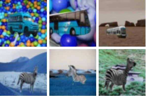
(b) COCO-on-Places

(c) BAR

Figure 3: For each dataset, the first two columns show bias-aligned (majority) samples, and the last column shows bias-conflicting (minority) samples. For BAR, the train set does not contain any bias-conflicting samples.

Biased MNIST [62]. As shown in Fig. 3(a), Biased MNIST requires classifying MNIST digits while remaining robust to multiple sources of biases, including color, texture, scale, and contextual biases. This is more challenging than the widely used Colored MNIST dataset [5, 34, 40], where the only source of bias is the spuriously correlated color. In our work, we build on the version created in [62]. We use $160\times 160$ images with $5\times 5$ grids of cells, where the target digit is placed in one of the grid cells and is spuriously correlated with: a) digit size/scale (number of cells a digit occupies), b) digit color, c) type of background texture, d) background texture color, e) co-occurring letters, and f) colors of the co-occurring letters. Following [62], we denote the probability with which each digit co-occurs with its biased property in the training set by $p_{bias}$. For instance, if $p_{bias}=0.95$, then 95% of the digit 1s are red, 95% of digit 1s co-occur with letter ‘a’ (not necessarily colored red) and so on. We set $p_{bias}$ to 0.95 for all the experiments. The validation and test sets are unbiased. Biased MNIST has 10 classes and 50K train, 10K validation, and 10K test samples.

COCO-on-Places [3]. As shown in Fig. 3(b), COCO-on-Places puts COCO objects [41] on spuriously correlated Places backgrounds [78]. For instance, buses mostly appear in front of balloons and birds in front of trees. The dataset provides three different test sets: a) biased backgrounds (in-distribution), which reflects the object-background correlations present in the train set, b) unseen backgrounds (non-systematic shift), where the objects are placed on backgrounds that are absent from the train set and c) seen, but unbiased backgrounds (systematic shift) where the objects are placed on backgrounds that were not spuriously correlated with the objects in the train set. Results in [3] show it is difficult to maintain high accuracy on both the in-distribution and shifted-distribution test sets. Apart from that, COCO-on-Places also includes an anomaly detection task, where anomalous samples from unseen object class need to be distinguished from the in-distribution samples. COCO-on-Places has 9 classes with 7200 train, 900 validation, and 900 test images.

Biased Action Recognition (BAR) [47]. BAR reflects real world challenges where bias attributes are not explicitly labeled for debiasing algorithms, with the test set containing additional correlations not seen during training. The dataset consists of correlated action-background pairs, where the train set consists of selected action-background pairs, e.g., climbing on a rock, whereas the evaluation set consists of differently correlated action-background pairs, e.g., climbing on snowy slopes (see Fig. 3(c)). The background is not labeled for the debiasing algorithms, making it a challenging benchmark. BAR has 6 classes with 1941 train and 654 test samples.

4.2 Comparison Methods

We compare OccamNets with four state-of-the-art bias mitigation methods, apart from the vanilla empirical risk minimization procedure:

• Empirical Risk Minimization (ERM) is the default method used by most deep learning models and it often leads to dataset bias exploitation since it minimizes the train loss without any debiasing procedure.

• Spectral Decoupling (SD) [51] applies regularization to model outputs to help decouple features. This can help the model focus more on the signal.

• Group Upweighting (Up Wt) balances the loss contributions from the majority and the minority groups by multiplying the loss by $\frac{1}{n_{g}^{\gamma}}$, where $n_{g}$ is the number of samples in group $g$ and $\gamma$ is a hyper-parameter.

• Group DRO (gDRO) [55] is an instance of a broader family of distributionally robust optimization techniques [18, 48, 52], that optimizes for the difficult groups in the dataset.

• Predictive Group Invariance (PGI) [3] is another grouping method, that encourages matched predictive distributions across easy and hard groups within each class. It penalizes the KL-divergence between predictive distributions from within-class groups.

Dataset Sub-groups. For debiasing, Up Wt, gDRO, and PGI require additional labels for covariates (sub-group labels). Past work has focused on these labels being supplied by an oracle; however, having access to all relevant sub-group labels is often impractical for large datasets. Some recent efforts have attempted to infer these sub-groups. Just train twice (JTT) [42] uses a bias-prone ERM model by training for a few epochs to identify the difficult groups. Environment inference for invariant learning (EIIL) [14] learns sub-group assignments that maximize the invariant risk minimization objective [5]. Unfortunately, inferred sub-groups perform worse in general than when they are supplied by an oracle [3, 42]. For the methods that require them, which excludes OccamNets, we use oracle group labels (i.e., for Biased MNIST and COCO-on-Places). Inferred group labels are used for BAR, as oracle labels are not available.

For Biased MNIST, all the samples having the same class and the same value for all of the spurious factors are placed in a single group. For COCO-on-Places, objects placed on spuriously correlated backgrounds form the majority group, while the rest form the minority group. BAR does not specify oracle group labels, so we adopt the JTT method. Specifically, we train an ERM model for single epoch, reserving 20% of the samples with the highest losses as the difficult group and the rest as the easy group. We chose JTT over EIL for its simplicity. OccamNets, of course do not require such group labels to be specified.

Architectures. ResNet-18 is used as the standard baseline architecture for our studies. We compare it with an OccamNet version of ResNet-18, i.e., OccamResNet-18. To create this architecture, we add early exit modules to each of ResNet-18’s convolutional blocks. To keep the number of parameters in OccamResNet-18 comparable to ResNet-18, we reduce the feature map width from 64 to 48. Assuming 1000 output classes, ResNet-18 has 12M parameters compared to 8M in OccamResNet-18. Further details are provided in Sec. A.7.

4.3 Metrics and Model Selection

We report the means and standard deviations of test set accuracies computed across five different runs for all the datasets. For Biased MNIST, we report the unbiased test set accuracy (i.e., $p_{bias}=0.1$) alongside the majority and minority group accuracies for each bias variable. For COCO-on-Places, unless otherwise specified, we report accuracy on the most challenging test split: with seen, but unbiased backgrounds. We also report the average precision score to measure the ability to distinguish 100 anomalous samples from the in-distribution samples for the anomaly detection task of COCO-on-Places. For BAR, we report the overall test accuracies. We use unbiased validation set of Biased MNIST and validation set with unbiased backgrounds for COCO-on-Places for hyperparameter tuning. The hyperparameter search grid and selected values are specified in Sec. A.8.

5 Results and Analysis

5.1 Overall Results

Table 1: Unbiased test set accuracies comparing OccamResNet to the more conventional ResNet architectures without early exits and constrained class activation maps. We format the first, second and $\underline{third}$ best results.

Architecture+Method	Biased MNIST	COCO-on-Places	BAR
Results on Standard ResNet-18
ResNet+ERM	36.8 $\pm$ 0.7	35.6 $\pm$ 1.0	51.3 $\pm$1.9
ResNet+SD [51]	37.1 $\pm$ 1.0	35.4 $\pm$ 0.5	51.3 $\pm$2.3
ResNet+Up Wt	37.7 $\pm$ 1.6	35.2 $\pm$ 0.4	51.1 $\pm$1.9
ResNet+gDRO [56]	19.2 $\pm$ 0.9	35.3 $\pm 0.1$	38.7 $\pm$2.2
ResNet+PGI [3]	48.6 $\pm$ 0.7	42.7 $\pm$ 0.6	53.6 $\pm$0.9
Results on OccamResNet-18
OccamResNet	65.0 $\pm 1.0$	43.4 $\pm$ 1.0	52.6 $\pm$1.9

OccamNets vs. ERM and Recent Bias Mitigation Methods. To examine how OccamNets fare against ERM and state-of-the-art bias mitigation methods, we run the comparison methods on ResNet and compare the results with OccamResNet. Results are given in Table 1. OccamResNet outperforms state-of-the-art methods on Biased MNIST and COCO-on-Places and rivals PGI on BAR, demonstrating that architectural inductive biases alone can help mitigate dataset bias. The gap between OccamResNet and other methods is large on Biased MNIST (16.4 - 46.0% absolute difference). For COCO-on-Places, PGI rivals OccamResNet, and clearly outperforms all other methods, in terms of accuracy on the test split with seen, but unbiased backgrounds. OccamResNet’s results are impressive considering that Up Wt, gDRO, and PGI all had access to the bias group variables, unlike OccamNet, ERM, and SD.

Combining OccamNets with Recent Bias Mitigation Methods. Because OccamNets are a new network architecture, we used OccamResNet-18 with each of the baseline methods instead of ResNet-18. These results are shown in Table 2, where we provide unbiased accuracy along with any improvement or impairment of performance when OccamResNet-18 is used instead of ResNet-18. All methods benefit from using the OccamResNet architecture compared to ResNet-18, with gains of 10.6% - 28.2% for Biased MNIST, 0.9% - 7.8% for COCO-on-Places, and 1.0% - 14.2% for BAR.

Table 2: Unbiased accuracies alongside  improvement/ impairment when the comparison methods are run on OccamResNet instead of ResNet.

Architecture+Method	Biased MNIST	COCO-on-Places	BAR
OccamResNet	65.0 (+28.2)	43.4 (+7.8)	52.6 (+1.3)
OccamResNet +SD [51]	55.2 (+18.1)	39.4 (+4.0)	52.3 (+1.0)
OccamResNet +Up Wt	65.7 (+28.0)	42.9 (+7.7)	52.2 (+1.1)
OccamResNet +gDRO [56]	29.8 (+10.6)	40.7 (+5.4)	52.9 (+14.2)
OccamResNet +PGI [3]	69.6 (+21.0)	43.6 (+0.9)	55.9 (+2.3)

5.2 Analysis of the Proposed Inductive Biases

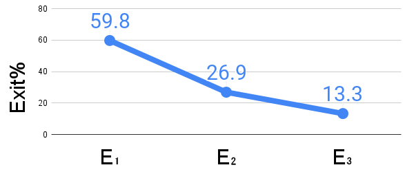
(a) Biased MNIST

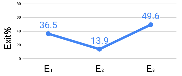
(b) COCO-on-Places

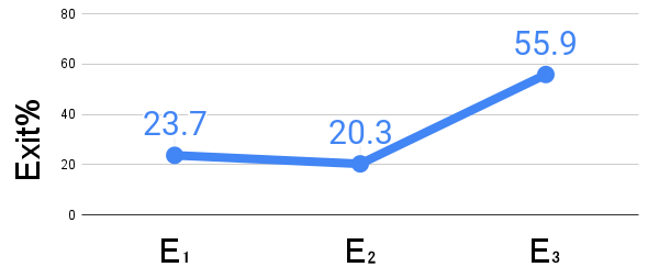
(c) BAR

Figure 4: Percentage of samples exited (Exit%) from each exit (barring $E_{0}$).

In this section, we analyze the impacts of each of the proposed modifications in OccamNets and their success in achieving the desired behavior.

Analysis of Early Exits. OccamResNet has four exits, the first exit is used for bias amplification and the rest are used to potentially exit early during inference. To analyze the usage of the earlier exits, we plot the percentage of samples that exited from each exit in Fig. 4. For Biased MNIST dataset, a large portion of the samples, i.e., 59.8% exit from the shallowest exit of $E_{1}$ and only 13.3% exit from the final exit $E_{3}$. For COCO-on-Places and BAR, 50.4% and 44.1% samples exit before $E_{3}$, with 49.6% and 55.9% samples using the full depth respectively. These results show that the OccamNet s favor exiting early, but that they do use the full network depth if necessary.

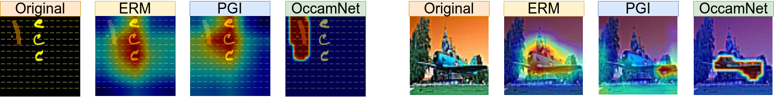
Figure 5: Original image, and Grad-CAM visualizations for ERM and PGI on ResNet, and CAM visualizations on OccamResNet. The visualizations are for the ground truth.

CAM Visualizations. To compare the localization capabilities of OccamResNets to ResNets, we present CAM visualizations in Fig. 5. For ResNets that were run with ERM and PGI, we show Grad-CAM visualizations [60], whereas for OccamResNets, we directly visualize the CAM heatmaps obtained from the earliest exit used for each sample. As shown in the figure, OccamResNet generally prefers smaller regions that include the target object. On the other hand, comparison methods tend to focus on larger visual regions that include irrelevant object/background cues leading to lower accuracies.

Table 3: Ablation Studies on OccamResNet

Ablation Description	Biased MNIST	COCO-on-Places
Using only one exit at the end	35.9	35.0
Weighing all the samples equally i.e., $\mathcal{W}_{j}=1$	66.3	40.8
Without the CAM suppression loss i.e., $\lambda_{CS}=0$	48.2	37.1
Full OccamResNet	65.0	43.4

Ablations. To study the importance of the introduced inductive biases, we perform ablations on Biased MNIST and COCO-on-Places. First, to examine if the multi-exit setup is helpful, we train networks with single exit attached to the end of the network. This caused accuracy drops of 29.1% on Biased MNIST and 8.4% on COCO-on-Places, indicating that the multi-exit setup is critical. To examine if the weighted output prediction losses are helpful or harmful, we set all the loss weights ($\mathcal{W}_{j}$) to 1. This resulted in an accuracy drop of 2.6% on COCO-on-Places. However, it improved accuracy on Biased MNIST by 1.3%. We hypothesize that since the earlier exits suffice for a large number of samples in Biased MNIST (as indicated in Fig. 4(a)), the later exits may not receive sufficient training signal with the weighted output prediction losses. Finally, we ran experiments without the CAM suppression loss by setting $\lambda_{CS}$ to 0. This caused large accuracy drops of 16.8% on Biased MNIST and 6.3% on COCO-on-Places. These experiments demonstrate that both inductive biases are vital for OccamNets.

5.3 Robustness to Different Types of Shifts

A robust system must handle different types of bias shifts. To test this ability, we examine the robustness to each bias variable in Biased MNIST and we also compare the methods on the differently shifted test splits of COCO-on-Places.

In Table 4, we compare how ResNet and OccamResNet are affected by the different bias variables in Biased MNIST. For this, we present majority and minority group accuracies for each variable. Bias variables with large differences between the majority and the minority groups, i.e., large majority/minority group discrepancy (MMD) are the most challenging spurious factors. OccamResNet s, with and without PGI, improve on both majority and minority group accuracies across all the bias variables. OccamResNets are especially good at ignoring the distracting letters and their colors, obtaining MMD values between 0-1%. ResNets, on the other hand are susceptible to those spurious factors, obtaining MMD values between 7.9-20.7%. Among all the variables, digit scale and digit color are the most challenging ones and OccamResNets mitigate their exploitation to some extent.

Table 4: Accuracies on majority (maj)/minority (min) groups for each bias variable in Biased MNIST ($p_{bias}=0.95$). We embolden the results with the lowest differences between the groups.

Architecture+Method		Digit Scale	Digit Color	Texture	Texture Color	Letter	Letter Color
	Test Acc.	maj/min	maj/min	maj/min	maj/min	maj/min	maj/min
ResNet+ERM	36.8	87.2/31.3	78.5/32.1	76.1/32.4	41.9/36.3	46.7/35.7	45.7/35.9
ResNet+PGI	48.6	91.9/43.8	84.8/44.6	79.5/45.1	51.3/48.3	67.2/46.5	55.8/47.9
OccamResNet	65.0	94.6/61.7	96.3/61.5	81.6/63.1	66.8/64.8	64.7/65.1	64.7/65.1
OccamResNet+PGI	69.6	95.4/66.7	97.0/66.5	88.6/67.4	71.4/69.4	69.6/69.6	70.5/69.5

Table 5: Accuracies on all three test splits of COCO-on-Places, alongside mean average precision for the anomaly detection task.

Architecture+Method	Biased Backgrounds	Unseen Backgrounds	Seen, but Non-Spurious Backgrounds	Anomaly Detection
Results on Standard ResNet-18
ResNet+ERM	84.9 $\pm$ 0.5	53.2 $\pm$0.7	35.6 $\pm$1.0	20.1 $\pm$1.5
ResNet+PGI [3]	77.5 $\pm$0.6	52.8 $\pm$0.7	42.7 $\pm$0.6	20.6 $\pm$2.1
Results on OccamResNet-18
OccamResNet	84.0 $\pm$1.0	55.8 $\pm$1.2	43.4 $\pm$1.0	22.3 $\pm$2.8
OccamResNet +PGI [3]	82.8 $\pm$0.6	55.3 $\pm$1.3	43.6 $\pm$ 0.6	21.6 $\pm$1.6

Next, we show accuracies for base method and PGI on both ResNet-18 and OccamResNet-18 on all of the test splits of COCO-on-Places in Table 5. The different test splits have different kinds of object-background combinations, and ideally the method should work well on all three test splits. PGI run on ResNet-18 improves on the split with seen, but non-spurious backgrounds but incurs a large accuracy drop of 7.4% on the in-distribution test set, with biased backgrounds. On the other hand, OccamResNet-18 shows only 0.9% drop on the biased backgrounds, while showing 2.6% accuracy gains on the split with unseen backgrounds and 7.8% accuracy gains on the split with seen, but non-spurious backgrounds. It further obtains 2.2% gains on the average precision metric for the anomaly detection task. PGI run on OccamResNet exhibits a lower drop of 2.1% on the in-distribution split as compared to the PGI run on ResNet, while obtaining larger gains on rest of the splits. These results exhibit that OccamNets obtain high in-distribution and shifted-distribution accuracies.

5.4 Evaluation on Other Architectures

To examine if the proposed inductive biases improve bias-resilience in other architectures too, we created OccamEfficientNet-B2 and OccamMobileNet-v3 by modifying EfficientNet-B2 [65] and MobileNet-v3 [28, 29]. OccamNet variants outperform standard architectures on both Biased MNIST (OccamEfficientNet-B2: 59.2 vs. EfficientNet-B2: 34.4 and OccamMobileNet-v3: 49.9 vs. MobileNet-v3: 40.4) and COCO-on-Places (OccamEfficientNet-B2: 39.2 vs. EfficientNet-B2: 34.2 and OccamMobileNet-v3: 40.1 vs. MobileNet-v3: 34.9). The gains show that the proposed modifications improve robustness in other commonly used architectures too. We provide the detailed results in Sec. A.6.

5.5 Do OccamNets Work on Less Biased Datasets?

To examine if OccamNets also work well on datasets with less bias, we train ResNet-18 and OccamResNet-18 on 100 classes of the ImageNet dataset [16]. OccamResNet-18 obtains competitive numbers compared to the standard ResNet-18 (OccamResNet-18: 92.1, vs. ResNet-18: 92.6, top-5 accuracies). However, as described in rest of this paper, OccamResNet-18 achieves this with improved resistance to bias (e.g., if the test distributions were to change in future). Additionally, it also reduces the computations with 47.6% of the samples exiting from $E_{1}$ and 13.3% of samples exiting from $E_{2}$. As such, OccamNets have the potential to be the de facto network choice for visual recognition tasks regardless of the degree of bias.

6 Discussion

Relation to Mixed Capacity Models. Recent studies have shown that sufficiently simple models, e.g., models with a limited number of parameters [13, 27] or models trained for a few epochs [42, 71] amplify biases. Specifically, [27] shows that model compression disproportionately hampers minority samples. Seemingly, this is an argument against smaller models (simpler hypotheses), i.e., against Occam’s principles. However, [27] does not study network depth, unlike our work. Our paper suggests that using only the necessary capacity for each example yields greater robustness.

Relation to Multi-Hypothesis Models. Some recent works generate multiple plausible hypotheses [39, 68] and use extra information at test time to choose the best hypothesis. The techniques include training a set of models with dissimilar input gradients [68] and training multiple prediction heads that disagree on a target distribution [39]. An interesting extension of OccamNets could be making diverse predictions through the multiple exits and through CAMs that focus on different visual regions. This could help avoid discarding complex features in favor of simpler ones [61]. This may also help with under-specified tasks, where there are equally viable ways of making the predictions [39].

Other Architectures and Tasks. We tested OccamNets implemented with CNNs; however, they may be beneficial to other architectures as well. The ability to exit dynamically could be used with transformers, graph neural networks, and feed-forward networks more generally. There is some evidence already for this on natural language inference tasks, where early exits improved robustness in a transformer architecture [79]. While the spatial bias is more vision specific, it could be readily integrated into recent non-CNN approaches for image classification [17, 43, 69, 76].

6.1 Conclusion

In summary, the proposed OccamNets have architectural inductive biases favoring simpler solutions. The experiments show improvements over state-of-the-art bias mitigation techniques. Furthermore, existing methods tend to do better with OccamNets as compared to the standard architectures.

Acknowledgments.

This work was supported in part by NSF awards #1909696 and #2047556. The views and conclusions contained herein are those of the authors and should not be interpreted as representing the official policies or endorsements of any sponsor.

A Appendix

A.1 Detailed Results on Each Dataset

Biased MNIST. In Table A6, we present the unbiased test accuracies and majority/minority group accuracies for each bias variable. Methods run on Occam ResNet-18 lower the majority/minority discrepancy (MMD) compared to the methods run on ResNet-18 for all of the variables, indicating that OccamNets lower the tendencies to latch onto all of the spurious factors. OccamResNet-18 is especially robust to letter, letter color and texture color biases as shown by the low MMD values of $0-2.8\%$ compared to the larger MMD values obtained by ResNet-18.

Table A6: Accuracies on majority (maj)/minority (min) groups for each bias variable in Biased MNIST ($p_{bias}=0.95$).

Architecture+Method		Digit Scale	Digit Color	Texture	Texture Color	Letter	Letter Color
	Test Acc.	maj/min	maj/min	maj/min	maj/min	maj/min	maj/min
	Results on ResNet-18
ResNet+ERM	36.8	87.2/31.3	78.5/32.1	76.1/32.4	41.9/36.3	46.7/35.7	45.7/35.9
ResNet+SD [51]	37.1	83.4/32.0	76.9/32.7	76.7/32.7	42.3/36.6	48.3/35.8	48.9/35.9
ResNet+UpWt	37.7	88.0/32.1	80.4/32.9	75.6/33.4	41.9/37.2	46.7/36.6	46.9/36.7
ResNet+gDRO [56]	19.2	55.0/15.2	50.2/15.7	63.4/14.2	24.8/18.6	26.7/18.3	29.5/18.1
ResNet+PGI [3]	48.6	91.9/43.8	84.8/44.6	79.5/45.1	51.3/48.3	67.2/46.5	55.8/47.9
	Results on OccamResNet-18
OccamResNet	65.0	94.6/61.7	96.3/61.5	81.6/63.1	66.8/64.8	64.7/65.1	64.7/65.1
OccamResNet+SD [51]	55.2	92.3/51.1	92.9/50.9	78.9/52.5	57.4/54.9	55.9/55.1	55.3/55.2
OccamResNet+UpWt	65.7	95.1/62.5	96.3/62.3	82.4/63.9	68.3/65.5	65.3/65.8	65.3/65.8
OccamResNet+gDRO [56]	29.8	72.8/25.0	69.5/25.3	45.8/28.0	39.4/28.8	29.7/29.8	36.1/29.1
OccamResNet+PGI [3]	69.6	95.4/66.7	97.0/66.5	88.6/67.4	71.4/69.4	69.6/69.6	70.5/69.5

COCO-on-Places. In Table A7, we present the accuracies on each of the test splits of COCO-on-Places, alongside the average precision for the anomaly detection task. As discussed in 5.1, methods run on OccamResNet-18 show improvements over the methods run on ResNet-18 on the shifted test splits and the anomaly detection task. Furthermore, while PGI run on ResNet-18 shows a large drop of 7.4% on the in-distribution test split, methods (barring gDRO) run on OccamResNet-18 show smaller drops of $0.1-2.1\%$, indicating robustness to distributions consisting of the same or different biases as compared to the train distribution.

Table A7: Accuracy on the three splits of COCO-on-Places, alongside average precision for the anomaly detection task.

Methods	In- Distribution	Unseen Backgrounds	Seen, but Non-Spurious Backgrounds	Anomaly Detection
Results on ResNet-18
ResNet+ERM	84.9 $\pm$ 0.5	53.2 $\pm$0.7	35.6 $\pm$1.0	20.1 $\pm$1.5
ResNet+SD [51]	85.3 $\pm$0.3	52.8 $\pm$0.9	35.4 $\pm$0.5	19.9 $\pm$1.4
ResNet+UpWt	84.9 $\pm$0.6	52.3 $\pm$ 0.7	35.2 $\pm$ 0.4	20.4 $\pm$1.9
ResNet+gDRO [56]	81.6 $\pm$0.7	49.3 $\pm$1.3	35.3 $\pm$0.1	19.6 $\pm$1.7
ResNet+PGI [3]	77.5 $\pm$0.6	52.8 $\pm$0.7	42.7 $\pm$0.6	20.6 $\pm$2.1
Results on OccamResNet-18
OccamResNet	84.0 $\pm$1.0	55.8 $\pm$1.2	43.4 $\pm$1.0	22.3 $\pm$2.8
OccamResNet+SD [51]	84.8 $\pm$0.4	55.3 $\pm$0.5	39.4 $\pm$0.6	20.3 $\pm$1.0
OccamResNet+Up Wt	82.9 $\pm$0.5	56.6 $\pm$1.0	42.9 $\pm$0.8	21.0 $\pm$0.9
OccamResNet+gDRO [56]	78.6 $\pm$0.7	50.7 $\pm$2.0	40.7 $\pm$ 1.5	19.3 $\pm$2.3
OccamResNet+PGI [3]	82.8 $\pm$0.6	55.3 $\pm$1.3	43.6 $\pm$ 0.6	21.6 $\pm$1.6

BAR. First of all, BAR consists of only 1941 samples, so we pre-trained ResNet-18 and OccamResNet-18 on 100 classes of ImageNet (obtaining 92.6% and 92.1% top-5 accuracies respectively) before training on BAR. Without the pre-trained weights, BAR obtains 15-20% lower test set accuracies for both ResNet and OccamResNet as compared to the results with pre-trained weights. Now, as shown in Table A8, methods run on OccamResNet show gains in terms of the overall test set accuracies over the methods run on ResNet. The per-class standard deviations are larger (1.8-16.2%) as compared to the standard deviations for the overall test set accuracies (0.7-2.4%). That is, across the five different experiments run with different random seeds, the same methods run on the same architectures end up favoring different classes. We hypothesize that despite starting off from the same initial conditions i.e., the same pre-trained parameters, the randomness in the mini-batches drive the models to favor certain classes over the others. Tuning the optimizer e.g., switching to SGD, lowering the learning rates or increasing the weight decay can potentially help mitigate the unstable behavior.

Table A8: Overall and per-class accuracies on BAR

Methods	Overall	Climbing	Diving	Fishing	Pole Vaulting	Racing	Throwing
Results on ResNet-18
ResNet+ERM	51.3 $\pm 1.9$	69.5 $\pm 7.5$	29.2 $\pm 1.8$	39.9 $\pm 16.2$	55.5 $\pm 6.4$	75.6 $\pm 5.6$	31.8 $\pm 4.3$
ResNet+SD [51]	51.3 $\pm 2.3$	62.1 $\pm 7.5$	35.8 $\pm 2.0$	51.2 $\pm 6.4$	62.4 $\pm 9.2$	71.6 $\pm 10.0$	18.5 $\pm 6.7$
ResNet+Up Wt	51.1 $\pm 1.9$	61.7 $\pm 13.2$	43.9 $\pm 5.8$	42.3 $\pm 8.3$	52.3 $\pm 7.4$	67.9 $\pm 6.7$	28.2 $\pm 12.8$
ResNet+gDRO [56]	38.7 $\pm 2.2$	49.5 $\pm 8.5$	40.3 $\pm 8.4$	44.0 $\pm 10.4$	39.9 $\pm 7.1$	41.7 $\pm 4.0$	13.5 $\pm 5.9$
ResNet+PGI [3]	53.6 $\pm 0.9$	61.2 $\pm 10.4$	38.4 $\pm 4.1$	42.9 $\pm 8.4$	73.3 $\pm 3.7$	68.9 $\pm 5.9$	23.5 $\pm 1.9$
Results on OccamResNet-18
OccamResNet	52.6 $\pm 1.9$	59.3 $\pm 3.8$	42.3 $\pm 7.5$	44.6 $\pm 14.9$	60.5 $\pm 8.6$	74.1 $\pm 7.2$	22.1 $\pm 3.9$
OccamResNet+SD [51]	52.3 $\pm 2.4$	56.4 $\pm 6.8$	34.3 $\pm 5.8$	55.4 $\pm 7.4$	69.1 $\pm 4.9$	72.9 $\pm 4.2$	21.8 $\pm 2.1$
OccamResNet+Up Wt	52.2 $\pm 1.4$	57.9 $\pm 1.8$	35.7 $\pm 7.5$	51.8 $\pm 11.2$	64.3 $\pm 8.8$	71.8 $\pm 3.8$	27.4 $\pm 3.5$
OccamResNet+gDRO [56]	52.9 $\pm 0.8$	51.2 $\pm 9.6$	42.8 $\pm 8.2$	52.3 $\pm 5.1$	63.5 $\pm 7.3$	74.2 $\pm 5.2$	25.3 $\pm 4.5$
OccamResNet+PGI [3]	55.9 $\pm 0.7$	64.2 $\pm 5.1$	52.3 $\pm 6.4$	51.4 $\pm 8.3$	64.4 $\pm 4.1$	70.9 $\pm 8.1$	18.6 $\pm 6.8$

A.2 Early Exit Statistics

To examine the efficiency and robustness of each exit for all of the datasets, we present the exit %, accuracy on the exited samples and overall exit-wise accuracies on all the samples for OccamResNet-18 in Table A9. For Biased MNIST, the earliest exits $E_{1}$ and $E_{2}$ have high exit percentages of $59.8\%$ and $26.9\%$ respectively, alongside high accuracies on the exited samples: $68.1\%$ and $64.8\%$ respectively. These results show that OccamResNet has learned to identify and trigger earlier exits whenever appropriate. For COCO-on-Places, we observe large accuracies of 50.8% and 50.2% on the 13.9% and 49.6% samples exited from $E_{2}$ and $E_{3}$ respectively. The large percentage of samples exiting from $E_{3}$ shows that OccamResNet is capable of using the full network depth whenever needed. The accuracy on the samples that exited from $E_{1}$ is however low: 31.3%, even though the overall accuracy is 42.4%, indicating need for improvement in terms of training the earlier exit gates. We believe that tuning the training thresholds more comprehensively can potentially close this gap. Finally, for BAR, more than half i.e., 55.9% of the samples exit from $E_{3}$. The accuracies on the samples exited from $E_{1}$ and $E_{2}$: 55.0% and 65.3% are higher than the overall accuracies computed on all the samples i.e., 47.4% and 52.3% respectively. This again shows the ability to exit early whenever appropriate and the ability to utilize the full network depth only for the remaining samples.

Table A9: Percentage samples exited: (Exit %), accuracy (Acc.) on exited samples and accuracy on all the samples for each exit ($E_{j}$).

	Biased MNIST				COCO-on-Places				BAR
	$E_{0}$	$E_{1}$	$E_{2}$	$E_{3}$	$E_{0}$	$E_{1}$	$E_{2}$	$E_{3}$	$E_{0}$	$E_{1}$	$E_{2}$	$E_{3}$
Exit%	0.0	59.8	26.9	13.3	0.0	36.5	13.9	49.6	0.0	23.7	20.3	55.9
Acc. (exited)	N/A	68.1	64.8	52.1	N/A	31.3	50.8	50.2	N/A	55.0	65.3	46.6
Acc. (all)	12.7	65.1	65.5	65.5	10.0	42.4	43.4	41.4	26.5	47.4	52.3	52.5

Table A10: Exit comparison on models trained with different levels of biases on Biased MNIST. We present the percentage samples exited: (Exit %) and accuracy on all the samples for each exit ($E_{j}$).

	$p_{bias}=0.5$				$p_{bias}=0.95$
	$E_{0}$	$E_{1}$	$E_{2}$	$E_{3}$	$E_{0}$	$E_{1}$	$E_{2}$	$E_{3}$
Exit%	0.0	67.3	23.8	8.9	0.0	53.6	34.2	12.2
Acc. (all)	N/A	98.2	98.1	98.1	N/A	63.3	63.3	62.6

Table A11: Exit comparison on different test splits of COCO-on-Places. We present the percentage samples exited: (Exit %), accuracy (Acc.) on exited samples and accuracy on all the samples for each exit ($E_{j}$).

	In-Distribution				Unseen Backgrounds				Unbiased Backgrounds
	$E_{0}$	$E_{1}$	$E_{2}$	$E_{3}$	$E_{0}$	$E_{1}$	$E_{2}$	$E_{3}$	$E_{0}$	$E_{1}$	$E_{2}$	$E_{3}$
Exit%	0.0	54.6	12.4	33.0	0.0	13.1	9.7	77.2	0.0	39.4	14.5	46.1
Acc. (exited)	N/A	94.7	86.5	66.9	N/A	58.9	67.8	52.3	N/A	27.5	55.4	49.2
Acc. (all)	67.2	81.1	84.0	85.3	20.9	51.7	55.1	55.4	11.2	40.1	41.6	39.4

Exit Statistics on differently shifted distributions.

In general, we find that earlier exits are triggered more often for in-distribution (easier) test samples as compared to shifted distribution (more difficult) test samples. As shown in Table A10, for BiasedMNIST, when $p_{bias}$ is increased from $0.5$ (easy) to $0.95$ (hard), exit% of the earliest exit: $E_{1}$ drops from 67.3% to 53.6%. Similarly, as shown in Table A11, for COCO-on-Places, $E_{1}$’s exit% on in-distribution (easy) split is 54.6%, whereas it is 39.4% on unbiased backgrounds (hard) split. However, for the test split with unseen backgrounds, $E_{1}$’s exit%: 13.1% is lower than the exit% of 39.4% obtained for the test split with unbiased backgrounds, despite the latter being more difficult. OccamNet failed to trigger earlier exits even though $E_{1}$ was accurate for 51.7% of the samples $E_{2}$ was comparable with $E_{3}$ in terms of overall accuracy. We hypothesize that the earlier exits failed to trigger since they had not been trained to exit when the backgrounds are out-of-distribution. Thus, one area for improvement is to enable the ability to exit confidently in spite of the presence of previously unseen factors. Note that this analysis was performed on a single run, so may have small differences with the multi-run averages presented elsewhere.

A.3 Using comparable # of parameters

In the main paper, we compared OccamResNet-18 with 8M parameters (feature width = 48) and ResNet-18 with 12M parameters (feature width = 64). To examine if the lower number number of parameters is helping e.g., due to implicit regularization, we test an OccamResNet-18 with 12M parameters by setting the feature width to 58. As shown in Table A12, OccamResNet-18 with 12M parameters shows small improvements over OccamResNet-18 with 8M parameters in all the datasets. A more thorough analysis of model sizes and their impacts on accuracy is an interesting study and we leave this to future work.

Table A12: We train on OccamResNet-18-width-58 with 12M parameters (feature width set to 58) to make the number of parameters comparable to ResNet-18 (12M parameters, feature width=48).

Architecture+Method	Biased MNIST	COCO-on-Places	BAR
Results on Standard ResNet-18 (12M parameters, feature width=64)
ResNet+ERM	36.8 $\pm$ 0.7	35.6 $\pm$ 1.0	51.3 $\pm$1.9
ResNet+SD [51]	37.1 $\pm$ 1.0	35.4 $\pm$ 0.5	51.3 $\pm$2.3
ResNet+Up Wt	37.7 $\pm$ 1.6	35.2 $\pm$ 0.4	51.1 $\pm$1.9
ResNet+gDRO [56]	19.2 $\pm$ 0.9	35.3 $\pm 0.1$	38.7 $\pm$2.2
ResNet+PGI [3]	48.6 $\pm$ 0.7	42.7 $\pm$ 0.6	53.6 $\pm$0.9
Results on OccamResNet-18 (8M parameters, feature width=48)
OccamResNet	65.0 $\pm 1.0$	43.4 $\pm$ 1.0	52.6 $\pm$1.9
Results on OccamResNet-18-width-58 (12M parameters, feature width=58)
OccamResNet	65.9 $\pm 1.3$	43.8 $\pm$ 1.1	53.5 $\pm$2.2

A.4 Sample Complexity

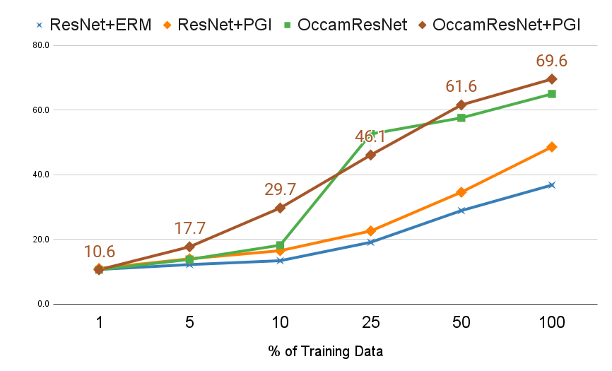
Figure A6: Unbiased accuracies obtained when trained with the indicated percent of training data.

It is desirable to have models that generalize despite being trained with a limited number of samples i.e., with reduced sample complexity. This is especially true for biased datasets, where reducing the train set size can amplify biases [72]. To study the ability to generalize when only a subset of the training data is available, we train ResNet and OccamResNet on ${1\%,5\%,10\%,25\%,50\%,100\%}$ of Biased MNIST’s train set. As shown in Fig. A6, OccamResNet (without PGI) trained on only 25% of the data outperforms ResNet+ERM and ResNet+PGI trained on 100% of the data showing increased sample complexity. When trained on only 10% of the training set, OccamResNet+PGI outperforms rest of the methods by large margins of $11.5-16.2\%$ showing that OccamResNet with group labels show the greatest efficacy in the low-shot data regime. When only 1% of the training data is available, all the methods obtain chance-level accuracies (i.e., near 10%) indicating lack of enough sufficient training samples for classification. For the rest, methods run on OccamResNet-18 outperform the methods run on ResNet-18, showing improved sample complexity.

A.5 Robustness to Varying Levels of Bias in Biased MNIST

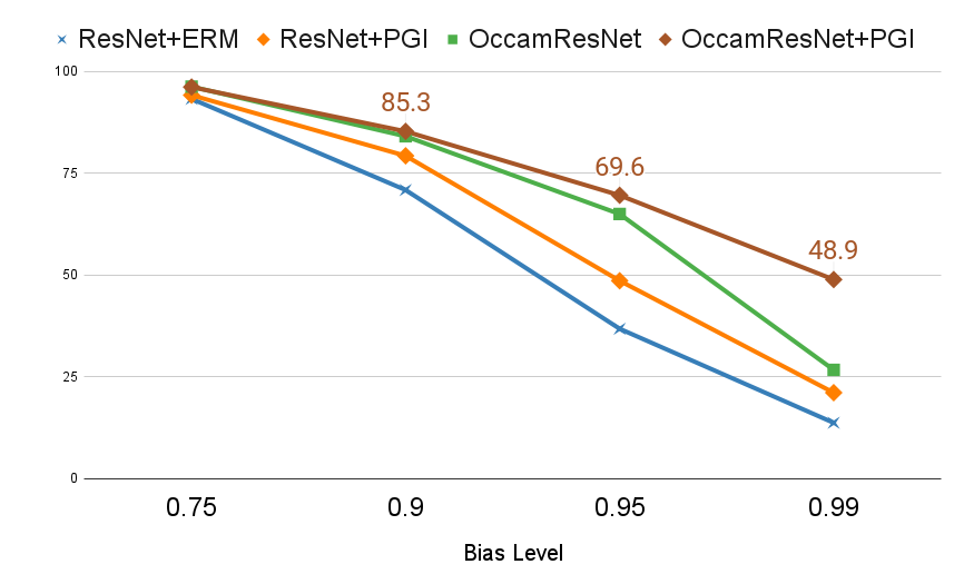
Figure A7: Unbiased accuracies at varying bias levels ($p_{bias}$) in Biased MNIST.

To gauge the robustness of models, it is important to examine their behaviors across varying levels of biases. For this, we present the unbiased accuracies obtained by training separate models on training sets with $p_{bias}\in\{0.75,0.9,0.95,0.99\}$. As shown in fig. A7, all of the methods obtain similar accuracies at $p_{bias}=0.75$, where bias is not severe. OccamResNet+PGI outperform rest of the methods at $p_{bias}=\{0.9,0.95,0.99\}$. The gap between OccamResNet+PGI and other methods are especially drastic for $p_{bias}=0.99$, indicating that when OccamResNet is trained to have similar prediction distributions across groups, it is capable of tackling highly biased training distributions too.

A.6 Evaluation on Other Architectures

Apart from ResNet, we also tested the proposed inductive biases on EfficientNet and MobileNet. The results are presented in Table A13. For both Biased MNIST and COCO-on-Places, Occam variants outperform the standard architectures, showing the efficacy of the proposed modifications.

Table A13: Unbiased test set accuracies comparing the standard and Occam variants of ResNet-18, EfficientNet-B2 and MobileNetv3 architectures, run without additional debiasing procedures.

Architecture	Number of Parameters	Biased MNIST	COCO-on-Places
ResNet-18	12M	36.8	35.6
OccamResNet-18	12M	65.9	43.8
EfficientNet-B2	9M	34.4	34.2
OccamEfficientNet-B2	9M	59.2	39.2
MobileNet-v3	5.5M	40.4	34.9
OccamMobileNet-v3	5.5M	49.9	40.1

A.7 OccamNet Implementation Details

In OccamNet, each exit module $E_{j}$ takes in feature maps produced by the corresponding block $B_{j}$ of the backbone network. $E_{j}$ consists of two $3\times 3$ convolutional layers $(F_{j})$ for the initial pre-processing of the feature maps. $F_{j}$ consists of convolutional layers with the number of channels set to: $max(\frac{d_{j}}{4},d_{min})$, where $d_{j}$ is the number of channels in the feature maps produced by $B_{j}$, and $d_{min}$ is set to 32 for OccamResNet and OccamMobileNet and 16 for OccamEfficientNet. Feature maps from $F_{j}$ are fed into the CAM predictor $C_{j}$ and the exit gate $G_{j}$. $C_{j}$ is a $1\times 1$ convolutional layer with the number of output channels set to the number of classes, $n_{Y}$. $G_{j}$ consists of a 16-dimensional hidden ReLU layer followed by a sigmoid layer that predicts the exit probability.

Exit Details. For convenience, we specify the exit locations with reference to PyTorch 1.7.1 implementations of the architectures. For ResNet, the residual layers that yield the same number of output channels are grouped together and we refer to each of those groups as a ‘block’. ResNet-18 consists of 4 blocks and we attach an exit to each of the blocks. For OccamResNet-18, with feature width of 58, the exit-wise input dimensions are: $E_{0}:58$, $E_{1}:116$, $E_{2}:232$ and $E_{3}:464$. Similarly, EfficientNet-B2 consists of 9 blocks and we attach the exits to the $3^{rd},5^{th},7^{th}~{}and~{}9^{th}$ blocks. We decrease the width multiplier of 1.1 in the standard architecture to 0.88 in OccamEfficientNet-B2 to create a model with comparable number of parameters of 9M for both. The input dimensions of the corresponding exits are: $E_{0}:24$, $E_{1}:72$, $E_{2}:168$ and $E_{3}:1120$. Finally, MobileNetv3-large consists of 17 blocks, and the exits are attached to the $2^{nd},7^{th},13^{th}$ and the $17^{th}$ blocks. We decrease the width multiplier from a value of $1$ in MobileNet-v3-large to 0.95 in OccamMobileNet-v3-large, so that both models have 5.5M parameters. The input dimensions of the corresponding exits are: $E_{0}:16,E_{1}:40,E_{2}:104,E_{3}:912$.

Modifications for COCO-on-Places. For COCO-on-Places, the images are small ($64\times 64$), so for ResNet-18 and OccamResNet-18, we replace the first convolutional layer (kernel size=$7$, padding=$3$, stride=$2$), with a smaller layer (kernel size=$3$, padding=$1$ and stride=$1$) and also remove the initial max pooling layer. For the standard and Occam variants of EfficientNet-B2 and MobileNet-v3, we scale up the image size to $224\times 224$, which improved the accuracy.

Computational Costs and Training Durations OccamResNet18 incurs additional multiply-accumulate (Mac) operations, requiring 2.11 GMacs compared to 1.82 GMacs required by ResNet18. While OccamResNet is slower than ERM on ResNet, it is faster than PGI run on ResNet. Average training durations per epoch for ERM on ResNet, PGI on ResNet and OccamResNet are: 10, 17, 14 secs for COCO-on-Places and 40, 67, 60 secs for BiasedMNIST on a Titan RTX.

A.8 Hyperparameters and Other Settings

In Table A14, we present the details about optimizers, training epochs and other hyperparameters for each method on each dataset. The hyperparameter search grids for OccamResNet-18 and all of the comparison methods are shown below. For each dataset, we tune ResNet-18 and OccamResNet-18 separately.

Spectral Decoupling (SD). The output decay term $\lambda$ is used to penalize the model predictions by using a regularizer: $\frac{\lambda}{2}||\hat{y}||^{2}_{2}$. We search for the output decay term $\lambda\in\{1,0.1,0.01,10^{-3},10^{-4}\}$.

Group Upweighting (UpWt). Group adjustment hyperparameter, i.e., the exponentiation factor $\gamma$ is used to balance the group-wise contributions $\frac{1}{n_{g}^{\gamma}}$, where $n_{g}$ is the number of samples in group $g$. We search for $\gamma\in\{0.5,1,2,3\}$.

Group DRO (gDRO). Again, we search for the group adjustment hyperparameter, i.e., $\gamma\in\{0.5,1,2,3\}$. Group weight step size, which is used to control the group-wise loss weights is selected by searching from these values: $\{0.1,0.01,10^{-3},10^{-4}\}$.

Predictive Group Invariance (PGI). The search range for the invariance penalty loss, i.e., the KLD loss between different groups from the same class is: {1, 10, 50, 100, 500, 1000}.

OccamNets. For OccamNets, we recommend tuning the accuracy threshold of the first exit: ($\tau_{acc,0}$) on a validation set, but fixing rest of the hyperparameters, based on the following observations:

• Bias Amplification Factor ($\gamma_{0}$) and Weight offset ($\epsilon$): We tuned $\gamma_{0}$ and $\epsilon$ on COCO-on-Places, but fixed the values for rest of the datasets. We observe that $\gamma_{0}\geq 3$ ensures sufficient bias amplification, so recommend using $\gamma_{0}=3$. Furthermore, $\epsilon=0.1$ ensures non-zero losses in all the datasets, so we recommend using this default value.

• Accuracy Thresholds ($\tau_{acc}$): We use arithmetic progression for the mean-per-class accuracy thresholds $\tau_{acc}$, with the difference $\Delta\tau_{acc,j}$, set to 0.1, i.e., the threshold is increased by $0.1$ every subsequent exit. We search for the initial training threshold $\tau_{acc,0}\in\{0.1,0.3,0.5\}$. BMNIST and COCO were relatively insensitive to $\tau_{acc,0}$, with absolute differences of only: 1-2% in accuracy and 1-4% in exit%. For BAR and ImageNet, we decreased $\tau_{acc,0}$ to $0.1$ since higher values increase exit% of $E_{1}$, which decreases the overall accuracy. So, we recommend tuning $\tau_{acc,0}$.

• Normalization term: The balancing/normalization in equation 4 can be generalized as $(\frac{1}{\sum_{1(g_{j}=k)}})^{\beta}$. We searched for $\beta$ in $\{0.5,1.0\}$. With $\beta=1$, only 8.8% samples exited from $E_{1}$ for BMNIST, compared to 59.8% with $\beta=0.5$. Accuracies for $\beta=$0.5/1.0 were similar: e.g., 65.0%/64.2% for BMNIST and 44.1%/44.0% for COCO (single runs), so we chose $\beta=0.5$ to favor earlier exits on all the datasets.

Table A14: Hyperparameters and other settings used for each method on all of the datasets.

Datasets/ Methods	Setting	Biased MNIST	COCO on Places	BAR
Common to all the methods	Optimizer	Adam	SGD	Adam
	Learning Rate (LR)	$10^{-3}$	0.1	5e-4
	LR Decay Milestones	[50,70]	[100,120,140]	-
	LR Decay Gamma	0.1	0.1	-
	Weight Decay	$5\times 10^{-4}$	$5\times 10^{-4}$	$5\times 10^{-4}$
	Momentum	-	0.9	-
	Batch Size	128	64	128
	Epochs	90	150	150
Spectral Decoupling (SD) on ResNet-18 [51]	Output Decay ($\lambda$)	$\lambda$ = 0.1	$\lambda_{min.}=10^{-3}$ $\lambda_{maj.}=0.1$	$\lambda=0.1$
Spectral Decoupling (SD) on OccamResNet-18 [51]	Output Decay ($\lambda$)	$\lambda$ = $10^{-3}$	$\lambda_{min.}=10^{-3}$ $\lambda_{maj.}=0.1$	$\lambda=10^{-3}$
Up Wt	Exponentiation Factor ($\gamma$)	2	1	1
Group DRO (gDRO) on ResNet-18 [56]	Step size	$10^{-3}$	$10^{-3}$	$0.01$
	Exponentiation Factor ($\gamma$)	$0.5$	$1$	$0.01$
Group DRO (gDRO) on OccamResNet-18 [56]	Step size	$10^{-3}$	$10^{-4}$	$0.01$
	Exponentiation Factor ($\gamma$)	$0.5$	$0.5$	$0.5$
Predictive Group Invariance (PGI) on ResNet-18 [3]	Invariance Loss Weight	100	50	10
Predictive Group Invariance (PGI) on OccamResNet-18 [3]	Invariance Loss Weight	50	1	50
OccamNets	Threshold for $E_{0}$ ($\tau_{acc,0}$)	0.5	0.5	0.1
	CAM Suppression Loss Weight ($\lambda_{CS}$)	0.1	0.1	0.1

A.9 Issues Training with GroupDRO (gDRO)

We find that gDRO on Biased MNIST and ResNet+gDRO on BAR obtain accuracies lower than ResNet+ERM. To alleviate this issue, we tried to tune the hyperparameters by lowering the learning rates to $\{10^{-4},10^{-5}\}$ and increasing the weight decays to $\{0.1,0.01,10^{-3}\}$ as suggested in [56], yet gDRO obtained low accuracies. We believe the challenge stems from the large number of dataset groups in Biased MNIST and the small training set size of BAR. While optimizing gDRO on such conditions still remains a challenge, gDRO run on OccamResNet showed accuracy gains of 10.6% on Biased MNIST and 14.2% on BAR over gDRO run on ResNet, indicating that OccamNets also offer better training process.

A.10 Augmentations

Biased MNIST. We do not perform any augmentation.

COCO-on-Places. Following [3], we apply random cropping by padding the original images by 8 pixels on all the sides (reflection padding) and taking $64\times 64$ random crops. We also apply random horizontal flips.

BAR. We apply random resized crops using a scale range of 0.7 to 1.0 and selecting aspect ratios between 1.0 to $\frac{4}{3}$. We also apply random horizontal flips.

A.11 Model Calibration

In Fig. A8 and  A9 we show the reliability diagrams for ERM model (leftmost column) and for each exit ($E1-E3$) for OccamResNet for COCO-on-Places and Biased MNIST respectively. In terms of model calibration, OccamNet reduces the expected calibration error (ECE) to some extent, yet there is a large room for improvement, which is an interesting direction to pursue.

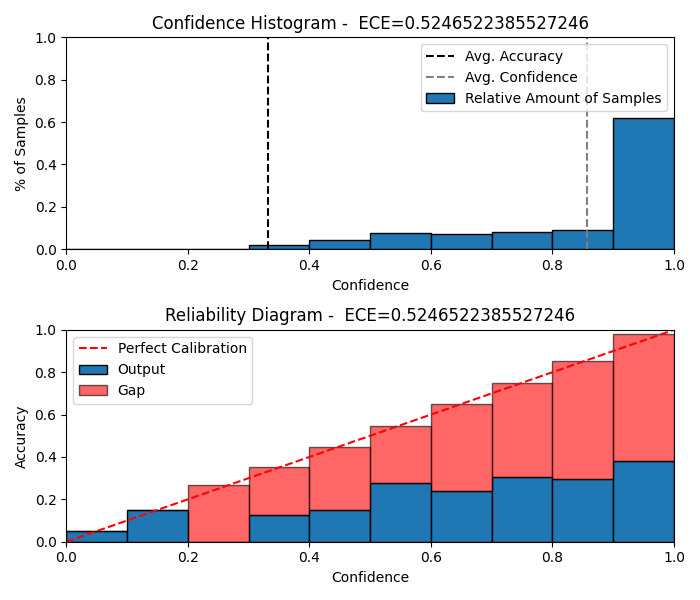
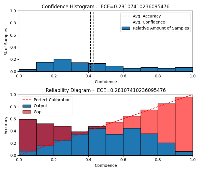
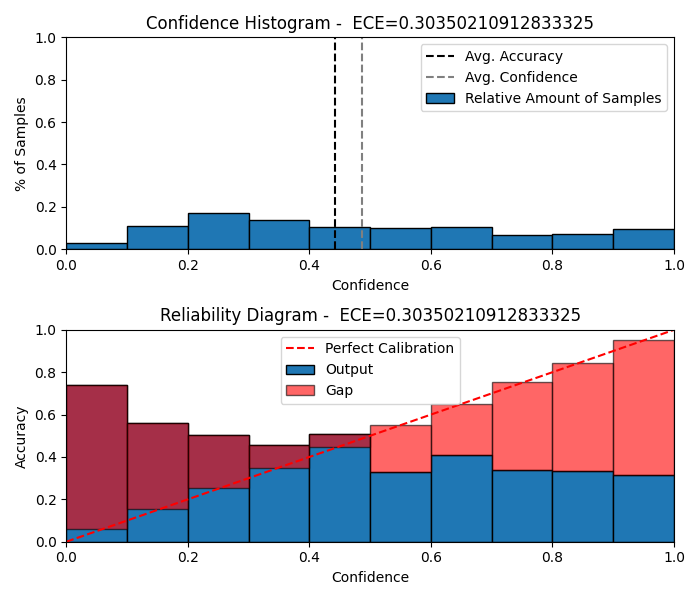
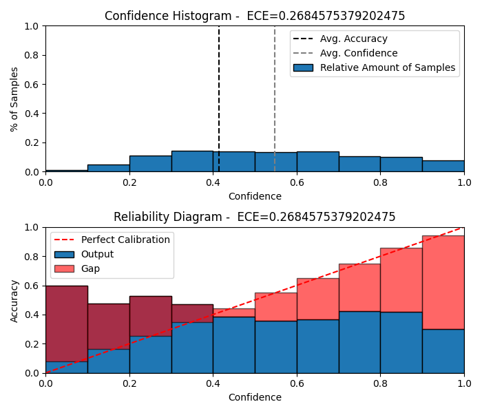
Figure A8: Reliability diagrams for the classifier trained with ERM (leftmost column) versus exit gate calibrations for $E1-E3$ (right hand columns) on COCO-on-Places (unbiased backgrounds test split).

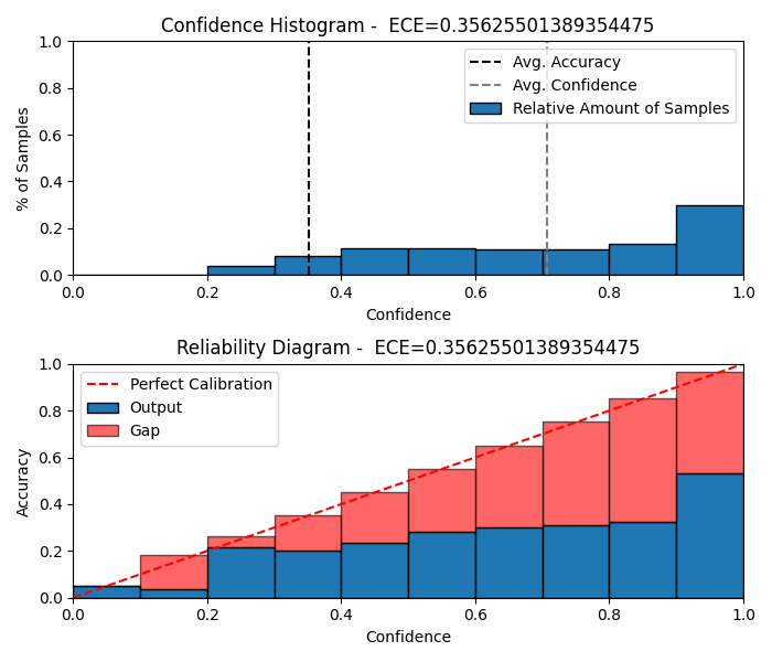
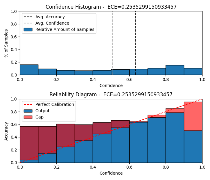
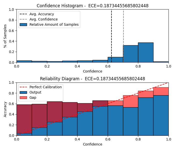
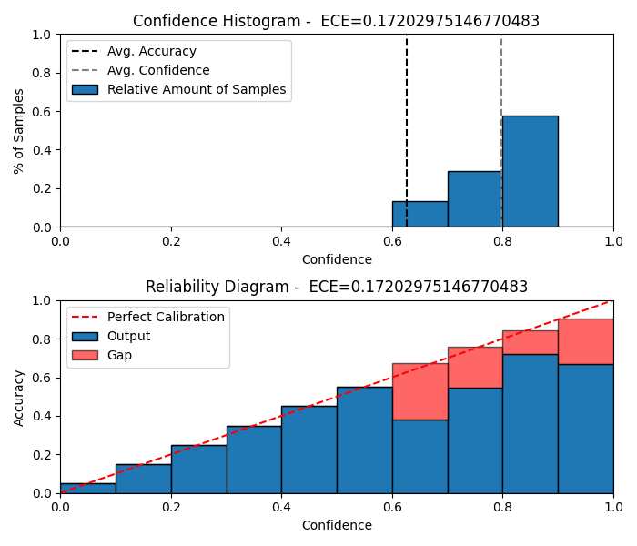
Figure A9: Reliability diagrams for the classifier trained with ERM (leftmost column) versus exit gate calibrations for $E1-E3$ (right hand columns) on Biased MNIST.

A.12 Other Architectures and Tasks.

We tested OccamNets implemented with CNNs; however, they may be beneficial to other architectures as well. The ability to exit dynamically could be used with transformers, graph neural networks, and feed-forward networks more generally. There is some evidence already for this on natural language inference tasks, where early exits improved robustness in a transformer architecture [79]. It would be interesting to evaluate multiple existing early exit mechanisms [59] for their abilities to discard spurious correlations. Furthermore, adapting the early exit ideas to non-classification tasks e.g., regression may require small changes e.g., exiting based on continuous error, which can be explored in future works.

References

- [1] Adeli, E., Zhao, Q., Pfefferbaum, A., Sullivan, E., Fei-Fei, L., Niebles, J.C., Pohl, K.: Bias-resilient neural network. ArXiv abs/1910.03676 (2019)
- [2] Agrawal, A., Batra, D., Parikh, D., Kembhavi, A.: Don’t just assume; look and answer: Overcoming priors for visual question answering. In: 2018 IEEE Conference on Computer Vision and Pattern Recognition, CVPR 2018, Salt Lake City, UT, USA, June 18-22, 2018. pp. 4971–4980. IEEE Computer Society (2018). https://doi.org/10.1109/CVPR.2018.00522
- [3] Ahmed, F., Bengio, Y., van Seijen, H., Courville, A.: Systematic generalisation with group invariant predictions. In: International Conference on Learning Representations (2020)
- [4] Anderson, P., He, X., Buehler, C., Teney, D., Johnson, M., Gould, S., Zhang, L.: Bottom-up and top-down attention for image captioning and visual question answering. In: 2018 IEEE Conference on Computer Vision and Pattern Recognition, CVPR 2018, Salt Lake City, UT, USA, June 18-22, 2018. pp. 6077–6086. IEEE Computer Society (2018). https://doi.org/10.1109/CVPR.2018.00636
- [5] Arjovsky, M., Bottou, L., Gulrajani, I., Lopez-Paz, D.: Invariant risk minimization. arXiv preprint arXiv:1907.02893 (2019)
- [6] Bolukbasi, T., Chang, K., Zou, J.Y., Saligrama, V., Kalai, A.T.: Man is to computer programmer as woman is to homemaker? debiasing word embeddings. In: Lee, D.D., Sugiyama, M., von Luxburg, U., Guyon, I., Garnett, R. (eds.) Advances in Neural Information Processing Systems 29: Annual Conference on Neural Information Processing Systems 2016, December 5-10, 2016, Barcelona, Spain. pp. 4349–4357 (2016)
- [7] Cadène, R., Dancette, C., Ben-younes, H., Cord, M., Parikh, D.: RUBi: Reducing Unimodal Biases for Visual Question Answering. In: Wallach, H.M., Larochelle, H., Beygelzimer, A., d’Alché-Buc, F., Fox, E.B., Garnett, R. (eds.) Advances in Neural Information Processing Systems 32: Annual Conference on Neural Information Processing Systems 2019, NeurIPS 2019, December 8-14, 2019, Vancouver, BC, Canada. pp. 839–850 (2019)
- [8] Chawla, N.V., Bowyer, K.W., Hall, L.O., Kegelmeyer, W.P.: Smote: synthetic minority over-sampling technique. Journal of artificial intelligence research 16, 321–357 (2002)
- [9] Chen, L., Yan, X., Xiao, J., Zhang, H., Pu, S., Zhuang, Y.: Counterfactual samples synthesizing for robust visual question answering. In: Proceedings of the IEEE/CVF Conference on Computer Vision and Pattern Recognition. pp. 10800–10809 (2020)
- [10] Chen, X., Dai, H., Li, Y., Gao, X., Song, L.: Learning to stop while learning to predict. In: International Conference on Machine Learning. pp. 1520–1530. PMLR (2020)
- [11] Choe, Y.J., Ham, J., Park, K.: An empirical study of invariant risk minimization. ICML 2020 Workshop on Uncertainty and Robustness in Deep Learning (2020)
- [12] Clark, C., Yatskar, M., Zettlemoyer, L.: Don’t take the easy way out: Ensemble based methods for avoiding known dataset biases. In: Proceedings of the 2019 Conference on Empirical Methods in Natural Language Processing and the 9th International Joint Conference on Natural Language Processing (EMNLP-IJCNLP). pp. 4069–4082. Association for Computational Linguistics, Hong Kong, China (2019). https://doi.org/10.18653/v1/D19-1418
- [13] Clark, C., Yatskar, M., Zettlemoyer, L.: Learning to model and ignore dataset bias with mixed capacity ensembles. In: Findings of the Association for Computational Linguistics: EMNLP 2020. pp. 3031–3045. Association for Computational Linguistics, Online (2020). https://doi.org/10.18653/v1/2020.findings-emnlp.272
- [14] Creager, E., Jacobsen, J.H., Zemel, R.: Environment inference for invariant learning. In: International Conference on Machine Learning. pp. 2189–2200. PMLR (2021)
- [15] Cui, Y., Jia, M., Lin, T., Song, Y., Belongie, S.J.: Class-balanced loss based on effective number of samples. In: IEEE Conference on Computer Vision and Pattern Recognition, CVPR 2019, Long Beach, CA, USA, June 16-20, 2019. pp. 9268–9277. Computer Vision Foundation / IEEE (2019). https://doi.org/10.1109/CVPR.2019.00949
- [16] Deng, J., Dong, W., Socher, R., Li, L.J., Li, K., Fei-Fei, L.: Imagenet: A large-scale hierarchical image database. In: 2009 IEEE conference on computer vision and pattern recognition. pp. 248–255. Ieee (2009)
- [17] Dosovitskiy, A., Beyer, L., Kolesnikov, A., Weissenborn, D., Zhai, X., Unterthiner, T., Dehghani, M., Minderer, M., Heigold, G., Gelly, S., et al.: An image is worth 16x16 words: Transformers for image recognition at scale. arXiv preprint arXiv:2010.11929 (2020)
- [18] Duchi, J.C., Hashimoto, T., Namkoong, H.: Distributionally robust losses against mixture covariate shifts. Under review (2019)
- [19] Duggal, R., Freitas, S., Dhamnani, S., Horng, D., Sun, J., et al.: Elf: An early-exiting framework for long-tailed classification. arXiv preprint arXiv:2006.11979 (2020)
- [20] Grand, G., Belinkov, Y.: Adversarial regularization for visual question answering: Strengths, shortcomings, and side effects. In: Proceedings of the Second Workshop on Shortcomings in Vision and Language. pp. 1–13. Association for Computational Linguistics, Minneapolis, Minnesota (2019). https://doi.org/10.18653/v1/W19-1801
- [21] Guo, M.H., Xu, T.X., Liu, J.J., Liu, Z.N., Jiang, P.T., Mu, T.J., Zhang, S.H., Martin, R.R., Cheng, M.M., Hu, S.M.: Attention mechanisms in computer vision: A survey. arXiv preprint arXiv:2111.07624 (2021)
- [22] He, H., Bai, Y., Garcia, E.A., Li, S.: Adasyn: Adaptive synthetic sampling approach for imbalanced learning. In: 2008 IEEE international joint conference on neural networks (IEEE world congress on computational intelligence). pp. 1322–1328. IEEE (2008)
- [23] He, H., Garcia, E.A.: Learning from imbalanced data. IEEE Transactions on knowledge and data engineering 21(9), 1263–1284 (2009)
- [24] He, K., Gkioxari, G., Dollár, P., Girshick, R.: Mask r-cnn. In: Proceedings of the IEEE international conference on computer vision. pp. 2961–2969 (2017)
- [25] He, K., Zhang, X., Ren, S., Sun, J.: Deep residual learning for image recognition. In: Proceedings of the IEEE conference on computer vision and pattern recognition. pp. 770–778 (2016)
- [26] Hettinger, C., Christensen, T., Ehlert, B., Humpherys, J., Jarvis, T., Wade, S.: Forward thinking: Building and training neural networks one layer at a time. arXiv preprint arXiv:1706.02480 (2017)
- [27] Hooker, S., Moorosi, N., Clark, G., Bengio, S., Denton, E.: Characterising bias in compressed models. arXiv preprint arXiv:2010.03058 (2020)
- [28] Howard, A., Sandler, M., Chu, G., Chen, L.C., Chen, B., Tan, M., Wang, W., Zhu, Y., Pang, R., Vasudevan, V., et al.: Searching for mobilenetv3. In: Proceedings of the IEEE/CVF International Conference on Computer Vision. pp. 1314–1324 (2019)
- [29] Howard, A.G., Zhu, M., Chen, B., Kalenichenko, D., Wang, W., Weyand, T., Andreetto, M., Adam, H.: Mobilenets: Efficient convolutional neural networks for mobile vision applications. arXiv preprint arXiv:1704.04861 (2017)
- [30] Hu, J., Shen, L., Albanie, S., Sun, G., Vedaldi, A.: Gather-excite: Exploiting feature context in convolutional neural networks. Advances in neural information processing systems 31 (2018)
- [31] Hu, T.K., Chen, T., Wang, H., Wang, Z.: Triple wins: Boosting accuracy, robustness and efficiency together by enabling input-adaptive inference. arXiv preprint arXiv:2002.10025 (2020)
- [32] Huang, G., Liu, Z., Van Der Maaten, L., Weinberger, K.Q.: Densely connected convolutional networks. In: Proceedings of the IEEE conference on computer vision and pattern recognition. pp. 4700–4708 (2017)
- [33] Jaderberg, M., Simonyan, K., Zisserman, A., et al.: Spatial transformer networks. Advances in neural information processing systems 28 (2015)
- [34] Kim, B., Kim, H., Kim, K., Kim, S., Kim, J.: Learning not to learn: Training deep neural networks with biased data. In: IEEE Conference on Computer Vision and Pattern Recognition, CVPR 2019, Long Beach, CA, USA, June 16-20, 2019. pp. 9012–9020. Computer Vision Foundation / IEEE (2019). https://doi.org/10.1109/CVPR.2019.00922
- [35] Kim, E., Lee, J., Choo, J.: Biaswap: Removing dataset bias with bias-tailored swapping augmentation. In: Proceedings of the IEEE/CVF International Conference on Computer Vision. pp. 14992–15001 (2021)
- [36] Krueger, D., Caballero, E., Jacobsen, J.H., Zhang, A., Binas, J., Zhang, D., Le Priol, R., Courville, A.: Out-of-distribution generalization via risk extrapolation (rex). In: International Conference on Machine Learning. pp. 5815–5826. PMLR (2021)
- [37] Lee, C.Y., Gallagher, P.W., Tu, Z.: Generalizing pooling functions in convolutional neural networks: Mixed, gated, and tree. In: Artificial intelligence and statistics. pp. 464–472. PMLR (2016)
- [38] Lee, C.Y., Xie, S., Gallagher, P., Zhang, Z., Tu, Z.: Deeply-supervised nets. In: Artificial intelligence and statistics. pp. 562–570. PMLR (2015)
- [39] Lee, Y., Yao, H., Finn, C.: Diversify and disambiguate: Learning from underspecified data. arXiv preprint arXiv:2202.03418 (2022)
- [40] Li, Y., Vasconcelos, N.: REPAIR: removing representation bias by dataset resampling. In: IEEE Conference on Computer Vision and Pattern Recognition, CVPR 2019, Long Beach, CA, USA, June 16-20, 2019. pp. 9572–9581. Computer Vision Foundation / IEEE (2019). https://doi.org/10.1109/CVPR.2019.00980
- [41] Lin, T.Y., Maire, M., Belongie, S., Hays, J., Perona, P., Ramanan, D., Dollár, P., Zitnick, C.L.: Microsoft coco: Common objects in context. In: European conference on computer vision. pp. 740–755. Springer (2014)
- [42] Liu, E.Z., Haghgoo, B., Chen, A.S., Raghunathan, A., Koh, P.W., Sagawa, S., Liang, P., Finn, C.: Just train twice: Improving group robustness without training group information. In: International Conference on Machine Learning. pp. 6781–6792. PMLR (2021)
- [43] Liu, Z., Lin, Y., Cao, Y., Hu, H., Wei, Y., Zhang, Z., Lin, S., Guo, B.: Swin transformer: Hierarchical vision transformer using shifted windows. In: Proceedings of the IEEE/CVF International Conference on Computer Vision. pp. 10012–10022 (2021)
- [44] Long, J., Shelhamer, E., Darrell, T.: Fully convolutional networks for semantic segmentation. In: Proceedings of the IEEE conference on computer vision and pattern recognition. pp. 3431–3440 (2015)
- [45] Mehrabi, N., Morstatter, F., Saxena, N., Lerman, K., Galstyan, A.: A survey on bias and fairness in machine learning. ACM Computing Surveys (CSUR) 54(6), 1–35 (2021)
- [46] Mostafa, H., Ramesh, V., Cauwenberghs, G.: Deep supervised learning using local errors. Frontiers in neuroscience p. 608 (2018)
- [47] Nam, J., Cha, H., Ahn, S., Lee, J., Shin, J.: Learning from failure: Training debiased classifier from biased classifier. In: Advances in Neural Information Processing Systems (2020)
- [48] Namkoong, H., Duchi, J.C.: Stochastic gradient methods for distributionally robust optimization with f-divergences. In: Lee, D.D., Sugiyama, M., von Luxburg, U., Guyon, I., Garnett, R. (eds.) Advances in Neural Information Processing Systems 29: Annual Conference on Neural Information Processing Systems 2016, December 5-10, 2016, Barcelona, Spain. pp. 2208–2216 (2016)
- [49] Nøkland, A.: Direct feedback alignment provides learning in deep neural networks. Advances in neural information processing systems 29 (2016)
- [50] Nøkland, A., Eidnes, L.H.: Training neural networks with local error signals. In: International conference on machine learning. pp. 4839–4850. PMLR (2019)
- [51] Pezeshki, M., Kaba, S.O., Bengio, Y., Courville, A., Precup, D., Lajoie, G.: Gradient starvation: A learning proclivity in neural networks. arXiv preprint arXiv:2011.09468 (2020)
- [52] Rahimian, H., Mehrotra, S.: Distributionally robust optimization: A review. arXiv preprint arXiv:1908.05659 (2019)
- [53] Ramakrishnan, S., Agrawal, A., Lee, S.: Overcoming language priors in visual question answering with adversarial regularization. In: Bengio, S., Wallach, H.M., Larochelle, H., Grauman, K., Cesa-Bianchi, N., Garnett, R. (eds.) Advances in Neural Information Processing Systems 31: Annual Conference on Neural Information Processing Systems 2018, NeurIPS 2018, December 3-8, 2018, Montréal, Canada. pp. 1548–1558 (2018)
- [54] Ronneberger, O., Fischer, P., Brox, T.: U-net: Convolutional networks for biomedical image segmentation. In: International Conference on Medical image computing and computer-assisted intervention. pp. 234–241. Springer (2015)
- [55] Sagawa, S., Koh, P.W., Hashimoto, T.B., Liang, P.: Distributionally robust neural networks for group shifts: On the importance of regularization for worst-case generalization. CoRR abs/1911.08731 (2019), http://arxiv.org/abs/1911.08731
- [56] Sagawa, S., Koh, P.W., Hashimoto, T.B., Liang, P.: Distributionally robust neural networks for group shifts: On the importance of regularization for worst-case generalization. arXiv preprint arXiv:1911.08731 (2019)
- [57] Sagawa, S., Raghunathan, A., Koh, P.W., Liang, P.: An investigation of why overparameterization exacerbates spurious correlations. In: Proceedings of the 37th International Conference on Machine Learning, ICML 2020, 13-18 July 2020, Virtual Event. Proceedings of Machine Learning Research, vol. 119, pp. 8346–8356. PMLR (2020)
- [58] Sanh, V., Wolf, T., Belinkov, Y., Rush, A.M.: Learning from others’ mistakes: Avoiding dataset biases without modeling them. arXiv preprint arXiv:2012.01300 (2020)
- [59] Scardapane, S., Scarpiniti, M., Baccarelli, E., Uncini, A.: Why should we add early exits to neural networks? Cognitive Computation 12(5), 954–966 (2020)
- [60] Selvaraju, R.R., Cogswell, M., Das, A., Vedantam, R., Parikh, D., Batra, D.: Grad-cam: Visual explanations from deep networks via gradient-based localization. In: Proceedings of the IEEE international conference on computer vision. pp. 618–626 (2017)
- [61] Shah, H., Tamuly, K., Raghunathan, A., Jain, P., Netrapalli, P.: The pitfalls of simplicity bias in neural networks. Advances in Neural Information Processing Systems 33 (2020)
- [62] Shrestha, R., Kafle, K., Kanan, C.: An investigation of critical issues in bias mitigation techniques. In: Proceedings of the IEEE/CVF Winter Conference on Applications of Computer Vision. pp. 1943–1954 (2022)
- [63] Singh, K.K., Mahajan, D., Grauman, K., Lee, Y.J., Feiszli, M., Ghadiyaram, D.: Don’t judge an object by its context: Learning to overcome contextual bias. In: 2020 IEEE/CVF Conference on Computer Vision and Pattern Recognition, CVPR 2020, Seattle, WA, USA, June 13-19, 2020. pp. 11067–11075. IEEE (2020). https://doi.org/10.1109/CVPR42600.2020.01108
- [64] Szegedy, C., Liu, W., Jia, Y., Sermanet, P., Reed, S., Anguelov, D., Erhan, D., Vanhoucke, V., Rabinovich, A.: Going deeper with convolutions. In: Proceedings of the IEEE conference on computer vision and pattern recognition. pp. 1–9 (2015)
- [65] Tan, M., Le, Q.: Efficientnet: Rethinking model scaling for convolutional neural networks. In: International conference on machine learning. pp. 6105–6114. PMLR (2019)
- [66] Teerapittayanon, S., McDanel, B., Kung, H.T.: Branchynet: Fast inference via early exiting from deep neural networks. In: 2016 23rd International Conference on Pattern Recognition (ICPR). pp. 2464–2469. IEEE (2016)
- [67] Teney, D., Abbasnejad, E., Hengel, A.v.d.: Unshuffling data for improved generalization. arXiv preprint arXiv:2002.11894 (2020)
- [68] Teney, D., Abbasnejad, E., Lucey, S., van den Hengel, A.: Evading the simplicity bias: Training a diverse set of models discovers solutions with superior ood generalization. arXiv preprint arXiv:2105.05612 (2021)
- [69] Tolstikhin, I.O., Houlsby, N., Kolesnikov, A., Beyer, L., Zhai, X., Unterthiner, T., Yung, J., Steiner, A., Keysers, D., Uszkoreit, J., et al.: Mlp-mixer: An all-mlp architecture for vision. Advances in Neural Information Processing Systems 34 (2021)
- [70] Torralba, A., Efros, A.A.: Unbiased look at dataset bias. In: The 24th IEEE Conference on Computer Vision and Pattern Recognition, CVPR 2011, Colorado Springs, CO, USA, 20-25 June 2011. pp. 1521–1528. IEEE Computer Society (2011). https://doi.org/10.1109/CVPR.2011.5995347
- [71] Utama, P.A., Moosavi, N.S., Gurevych, I.: Towards debiasing NLU models from unknown biases. In: Proceedings of the 2020 Conference on Empirical Methods in Natural Language Processing (EMNLP). pp. 7597–7610. Association for Computational Linguistics, Online (2020). https://doi.org/10.18653/v1/2020.emnlp-main.613, https://www.aclweb.org/anthology/2020.emnlp-main.613
- [72] Utama, P.A., Moosavi, N.S., Gurevych, I.: Towards debiasing NLU models from unknown biases. In: Proceedings of the 2020 Conference on Empirical Methods in Natural Language Processing (EMNLP). pp. 7597–7610. Association for Computational Linguistics, Online (2020). https://doi.org/10.18653/v1/2020.emnlp-main.613, https://www.aclweb.org/anthology/2020.emnlp-main.613
- [73] Venkataramani, S., Raghunathan, A., Liu, J., Shoaib, M.: Scalable-effort classifiers for energy-efficient machine learning. In: Proceedings of the 52nd Annual Design Automation Conference. pp. 1–6 (2015)
- [74] Wołczyk, M., Wójcik, B., Bałazy, K., Podolak, I., Tabor, J., Śmieja, M., Trzcinski, T.: Zero time waste: Recycling predictions in early exit neural networks. Advances in Neural Information Processing Systems 34 (2021)
- [75] Xu, K., Ba, J., Kiros, R., Cho, K., Courville, A., Salakhudinov, R., Zemel, R., Bengio, Y.: Show, attend and tell: Neural image caption generation with visual attention. In: International conference on machine learning. pp. 2048–2057. PMLR (2015)
- [76] Yu, W., Luo, M., Zhou, P., Si, C., Zhou, Y., Wang, X., Feng, J., Yan, S.: Metaformer is actually what you need for vision. arXiv preprint arXiv:2111.11418 (2021)
- [77] Zhang, B.H., Lemoine, B., Mitchell, M.: Mitigating unwanted biases with adversarial learning. In: Proceedings of the 2018 AAAI/ACM Conference on AI, Ethics, and Society. pp. 335–340 (2018)
- [78] Zhou, B., Lapedriza, A., Khosla, A., Oliva, A., Torralba, A.: Places: A 10 million image database for scene recognition. IEEE transactions on pattern analysis and machine intelligence 40(6), 1452–1464 (2017)
- [79] Zhou, W., Xu, C., Ge, T., McAuley, J., Xu, K., Wei, F.: Bert loses patience: Fast and robust inference with early exit. Advances in Neural Information Processing Systems 33, 18330–18341 (2020)