Shock interactions for the Burgers-Hilbert Equation

Abstract

This paper provides an asymptotic description of a solution to the Burgers-Hilbert equation in a neighborhood of a point where two shocks interact. The solution is obtained as the sum of a function with $H^{2}$ regularity away from the shocks plus a corrector term having an asymptotic behavior like $|x|\ln|x|$ close to each shock. A key step in the analysis is the construction of piecewise smooth solutions with a single shock for a general class of initial data.

1 Introduction

Consider the balance law obtained from Burgers’ equation by adding the Hilbert transform as a source term

$$u_{t}+\left({u^{2}\over 2}\right)_{x}~{}=~{}{\bf H}[u]\,.$$ (1.1)

This equation was derived in [1] as a model for nonlinear waves with constant frequency. Here the nonlocal source term

$${\bf H}[f](x)~{}\doteq~{}\lim_{\varepsilon\to 0+}{1\over\pi}\int_{|y|>\varepsilon}{f(x-y)\over y}\,dy$$

denotes the Hilbert transform of a function $f\in{\bf L}^{2}(\mathbb{R})$. It is well known [8] that ${\bf H}$ is a linear isometry from ${\bf L}^{2}(\mathbb{R})$ onto itself. Given any initial data

$$u(0,\cdot)~{}=~{}\bar{u}(\cdot)$$ (1.2)

with $\bar{u}\in H^{2}(\mathbb{R})$, the local existence and uniqueness of solutions to (1.1) was proved in [6], together with a sharp estimate on the time interval where this solution remains smooth. For a general initial data $\bar{u}\in{\bf L}^{2}(\mathbb{R})$, the global existence of entropy weak solutions to (1.1) was proved in [3], together with a partial uniqueness result. We remark that the well-posedness of the Cauchy problem for (1.1) remains a largely open question.

More recently, piecewise continuous solutions with a single shock have been constructed in [4]. As shown in Fig. 1, these solutions have the form

$$u(t,x)~{}=~{}w\bigl{(}t,x-y(t)\bigr{)}+\varphi\bigl{(}x-y(t)\bigr{)},$$ (1.3)

where $y(t)$ denotes the location of the shock at time $t$, and $w(t,\cdot)\in H^{2}\bigl{(}]-\infty,0[\,\cup\,]0,+\infty[\bigr{)}$ for all $t\geq 0$. Moreover, $\varphi$ is a fixed function with compact support, describing the asymptotic behavior of the solution near the shock. It is smooth outside the origin and satisfies

$$\varphi(x)~{}=~{}{2\over\pi}|x|\ln|x|\qquad\quad\hbox{for}\quad|x|\leq 1\,.$$ (1.4)

Remarkably, this “corrector term” $\varphi$ is universal, i.e., it does not depend on the particular solution of (1.1). The same analysis applies to solutions with finitely many, noninteracting shocks. In addition, the local asymptotic behavior of a solution up to the time when a new shock is formed was investigated in [9].

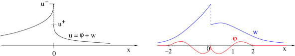
Figure 1: Decomposing a solution in the form (1.3)

The aim of the present note is to describe the asymptotic behavior of a solution in a neighborhood of a point where two shocks interact. Calling $T>0$ the time when the interaction takes place, our analysis splits into two parts. We first describe the behavior of the solution as $t\to T-$, i.e. as the two shocks approach each other. In a second step, to construct the solution for $t>T$, we solve a Cauchy problem with initial data given at $t=T$.

As it turns out, the profile $u(T,\cdot)$ is not “well prepared”, in the sense that it cannot be written in the form (1.3). To explain the difficulty, we recall that the solutions constructed in [4] had initial data of the form

$$u(0,x)~{}=~{}\overline{w}(x-y_{0})+\varphi(x-y_{0}),$$ (1.5)

for some $\overline{w}\in H^{2}\bigl{(}\mathbb{R}\setminus\{0\}\bigr{)}$ and $y_{0}\in\mathbb{R}$. These data are “well prepared”, in the sense that they already contain the corrector term $\varphi$. A natural class of initial data, not considered in [4], is

$$u(0,x)~{}=~{}\overline{w}(x-y_{0})\qquad\mathrm{with}\qquad\overline{w}\in H^{2}\bigl{(}\mathbb{R}\setminus\{0\}\bigr{)},\phantom{a}y_{0}\in\mathbb{R}.$$ (1.6)

By assumption, at time $t=0$ the derivative $u_{x}(0,x)~{}=~{}\overline{w}_{x}(x-y_{0})$ is piecewise continuous and uniformly bounded. However, in the solution to (1.1), (1.6), at each time $t>0$ we expect that $u_{x}(t,x)\to\pm\infty$ as $x\to y(t)\mp$. For this reason, the local construction of this solution requires a careful analysis. A more general class of initial data, containing both (1.5) and (1.6), as well as all profiles $u(T,\cdot)$ emerging from our shock interactions, will be studied in Section 2.

We recall here the definition of entropy weak solutions used in [3].

Definition 1.1

By an entropy weak solution of (1.1)-(1.2) we mean a function $u\in{\bf L}^{1}_{loc}([0,\infty[\,\times\mathbb{R})$ with the following properties.

• The map $t\mapsto u(t,\cdot)$ is continuous with values in ${\bf L}^{2}(\mathbb{R})$ and satisfies the initial condition (1.2).

• For any $k\in\mathbb{R}$ and every nonnegative test function $\phi\in{\cal C}^{1}_{c}(]0,\infty[\,\times\mathbb{R})$ one has

  $$\int\!\!\int\Big{[}|u-k|\phi_{t}+\Big{(}{u^{2}-k^{2}\over 2}\Big{)}\hbox{\rm sign}(u-k)\phi_{x}+H[u(t)](x)\hbox{\rm sign}(u-k)\phi\Big{]}\,dxdt~{}\geq~{}0.$$ (1.7)

The present paper will be concerned with a more regular class of solutions, which are piecewise continuous and can be determined by integrating along characteristics. These correspond to the “broad solutions” considered in [2, 7]. Throughout the sequel, the upper dot denotes a derivative w.r.t. time.

Definition 1.2

An entropy weak solution $u=u(t,x)$ of (1.1)-(1.2), defined on the interval $t\in[0,T]$, will be called a piecewise regular solution if there exist finitely many shock curves $y_{1}(t),\ldots,y_{n}(t)$ such that the following holds.

• For each $t\in[0,T]$, one has $u(t,\cdot)\in H^{2}\bigl{(}\mathbb{R}\setminus\{y_{1}(t),\ldots,y_{n}(t)\}\bigr{)}$.

• For each $i=1,\ldots,n$, the Rankine-Hugoniot conditions hold:

  $$u_{i}^{-}(t)~{}\doteq~{}u(t,y_{i}(t)-)~{}>~{}u(t,y_{i}(t)+)~{}\doteq~{}u_{i}^{+}(t),$$ (1.8)

  $$\dot{y}_{i}(t)~{}=~{}{u_{i}^{-}(t)+u_{i}^{+}(t)\over 2}\,.$$ (1.9)

• Along every characteristic curve $t\mapsto x(t)$ such that

  $$\dot{x}(t)~{}=~{}u\bigl{(}t,x(t)\bigr{)},$$ (1.10)

  one has

  $${d\over dt}u\bigl{(}t,x(t)\bigr{)}~{}=~{}{\bf H}[u](x(t)).$$ (1.11)

In the above setting, the Hilbert transform of the piecewise regular function $u(t,\cdot)$ can be computed using an integration by parts:

$${\bf H}[u(t)](x)~{}=~{}{1\over\pi}\int_{-\infty}^{\infty}u_{x}(t,y)\,\ln|x-y|\,dy+{1\over\pi}\sum_{i=1}^{n}\bigl{[}u_{i}^{+}(t)-u_{i}^{-}(t)\bigr{]}\,\ln\bigl{|}x-y_{i}(t)\bigr{|}\,.$$ (1.12)

The remainder of the paper is organized as follows. In Section 2 we state a local existence and uniqueness theorem for solutions to (1.1), valid for a class of initial data containing one single shock, but more general than in [4]. Towards the proof of Theorem 2.1, Section 3 develops various a priori estimates, while in Section 4 the local solution is constructed as a limit of a convergent sequence of approximations. As in [4], these are obtained by iteratively solving a sequence of linearized problems.

In the second part of the paper we study solutions of (1.1) with two shocks, up to the time of interaction. In Section 5 we perform some preliminary computations, motivating a particular form of the corrector term. In Section 6 we state and prove the second main result of the paper, Theorem 6.1, providing a detailed description of solutions up to the interaction time. This is achieved by a change of both time and space coordinates, so that the two shocks are located at the two points

$$x_{1}(t)~{}=~{}t~{}<~{}0~{}=~{}x_{2}(t),$$

and interact at time $t=0$. Our analysis shows that, at the interaction time, the solution profile contains a single shock and lies within the class of initial data covered by Theorem 2.1. Combining our two theorems, one thus obtains a complete description of the solution to (1.1) in a neighborhood of the interaction time.

2 Solutions with one shock and general initial data

Consider a piecewise regular solution of the Burgers-Hilbert equation (1.1), with one single shock. By the Rankine-Hugoniot condition, the location $y(t)$ of the shock at time $t$ satisfies

$$\dot{y}(t)~{}=~{}{u^{-}(t)+u^{+}(t)\over 2},\qquad u^{\pm}(t)~{}=~{}\lim_{x\to y(t)\pm}u(t,x).$$ (2.1)

As in [4], we shift the space coordinate, replacing $x$ with $x-y(t)$, so that in the new coordinate system the shock is always located at the origin. In these new coordinates, (1.1) takes the form

$$u_{t}+\left(u-{u^{-}(t)+u^{+}(t)\over 2}\right)u_{x}~{}=~{}{\bf H}[u].$$ (2.2)

In [4], given a “well prepared” initial data (1.5), a unique piecewise smooth entropy solution to (2.2) of the form

$$u(t,x)~{}=~{}w(t,x)+{2\eta(x)\over\pi}\cdot|x|\ln|x|\,,\qquad\qquad t>0\,$$

was constructed. Here $w(t,\cdot)\in H^{2}\bigl{(}\mathbb{R}\backslash\{0\}\bigr{)}$, while $\eta\in C^{\infty}(\mathbb{R})$ is an even cut-off function, satisfying

$$\left\{\begin{array}[]{rl}\eta(x)~{}=~{}1&\qquad\hbox{if}~{}~{}~{}|x|\leq 1,\\[2.84526pt] \eta(x)~{}=~{}0&\qquad\hbox{if}~{}~{}~{}|x|\geq 2,\\[2.84526pt] \eta^{\prime}(x)~{}\leq~{}0&\qquad\hbox{if}~{}~{}~{}x\geq 0\,.\end{array}\right.$$ (2.3)

For future use, it will be convenient to introduce the function

$$\phi(x,b)~{}\doteq~{}{2\eta(x)\over\pi}\cdot\Big{[}(|x|+b)\ln(|x|+b)-b\ln b\Big{]},\qquad\quad x\in\mathbb{R},~{}~{}b\geq 0.$$ (2.4)

Observe that

$$\phi(0,b)~{}=~{}0\qquad\qquad\hbox{for all}~{}~{}b\geq 0.$$ (2.5)

Our main goal in this section is to solve the Cauchy problem for (2.2) with initial data

$$u(0,x)~{}=~{}\overline{w}(x)+\overline{\varphi}(x),$$ (2.6)

where

$$\overline{w}\in H^{2}\bigl{(}\mathbb{R}\backslash\{0\}\bigr{)},\qquad\qquad\overline{\varphi}(x)~{}=~{}\Big{(}c_{1}\cdot\chi_{]-\infty,0[}+c_{2}\cdot\chi_{]0,+\infty[}\Big{)}\cdot\phi(x,0),$$ (2.7)

for some constants $c_{1}$, $c_{2}\in\mathbb{R}$. Note that this reduces to (1.5) in the case $c_{1}=c_{2}=1$.

To handle the more general initial data (2.6)-(2.7), we write the solution of (2.2) in the form

$$u(t,x)~{}=~{}w(t,x)+\varphi^{(w)}(t,x),$$ (2.8)

where the corrector term $\varphi^{(w)}(t,x)$ now depends explicitly on time $t$ and on the strength of the jump

$$\sigma^{(w)}(t)~{}\doteq~{}w^{-}(t)-w^{+}(t),\qquad\qquad w^{\pm}(t)\,\doteq\,w(t,0\pm).$$ (2.9)

To make an appropriate guess for the function $\varphi^{(w)}$, we observe that, by (1.12), the equation (2.2) can be approximated by the simpler equation

$$u_{t}+\left(u-{u^{-}(t)+u^{+}(t)\over 2}\right)u_{x}~{}=~{}{1\over\pi}(u^{+}(t)-u^{-}(t))\,\ln|x|.$$ (2.10)

Indeed, we expect that the solutions of (2.2) and (2.10) with the same initial data will have the same asymptotic structure near the origin. Their difference will lie in the more regular space $H^{2}\bigl{(}\mathbb{R}\backslash\{0\}\bigr{)}$. With this in mind, we thus make the ansatz

$$\varphi^{(w)}(t,x)~{}\doteq~{}\phi(x,0)+\Big{(}(c_{1}-1)\cdot\chi_{]-\infty,0[}+(c_{2}-1)\cdot\chi_{]0,+\infty[}\Big{)}\cdot\phi\left(x,\displaystyle{\sigma^{(w)}(t)t\over 2}\right).$$ (2.11)

Inserting (2.8) into (2.2), we obtain an equation for the remaining component $w(t,\cdot)$. Namely

$$w_{t}+a(t,x,w)\cdot w_{x}~{}=~{}F(t,x,w),$$ (2.12)

where $a$ and $F$ are given by

$$a(t,x,w)~{}=~{}w(t,x)+\varphi^{(w)}(t,x)-{w^{-}(t)+w^{+}(t)\over 2},$$ (2.13)

$$F(t,x,w)~{} = ~{}{\bf H}\left[\varphi^{(w)}\right](t,x)-\varphi^{(w)}\varphi^{(w)}_{x}(t,x)$$

$$+ \left({\bf H}\left[w\right](t,x)-\left[\varphi^{(w)}_{t}(t,x)+\left(w(t,x)-{w^{-}(t)+w^{+}(t)\over 2}\right)\cdot\varphi^{(w)}_{x}(t,x)\right]\right).$$

We observe that, in the present case of a solution with a single shock, by (2.5) the entropy admissibility condition (1.8) reduces to

$$w^{-}(t)~{}>~{}w^{+}(t).$$ (2.15)

Moreover, Definition 1.2 is satisfied provided that, along every characteristic curve $t\mapsto x(t;t_{0},x_{0})\not=0$ obtained by solving

$$\dot{x}(t)~{}=~{}a(t,x,w),\qquad\quad x(t_{0})\,=\,x_{0}\,,$$ (2.16)

one has

$$w(t_{0},x_{0})~{}=~{}\overline{w}\bigl{(}x(0;t_{0},x_{0})\bigr{)}+\int_{0}^{t_{0}}F\Big{(}t,x(t;t_{0},x_{0}),w\bigl{(}t,x(t;t_{0},x_{0})\bigr{)}\Big{)}\,dt\,.$$ (2.17)

The first main result of this paper provides the existence and uniqueness of an entropic solution, locally in time.

Theorem 2.1

For every $\overline{w}\in H^{2}\bigl{(}\mathbb{R}\setminus\{0\}\bigr{)}$ satisfying $\overline{w}(0-)-\overline{w}(0+)>0$ and every $c_{1}$, $c_{2}\in\mathbb{R}$, the Cauchy problem for the Burgers-Hilbert equation (1.1), with initial condition as in (2.6)-(2.7), admits a unique piecewise regular solution defined for $t\in[0,T]$, for some $T>0$ sufficiently small, depending only on $M_{0}$, $\delta_{0}$, $c_{1}$, and $c_{2}$.

The solution to the equivalent equation (2.12) will be obtained as a limit of a sequence of approximations. Namely, consider a sequence of linear approximations constructed as follows. As a first step, define

$$w_{1}(t,x)~{}=~{}\overline{w}(x)\qquad\qquad\hbox{for all}~{}~{}t\geq 0,~{}~{}x\in\mathbb{R}\,.$$ (2.18)

By induction, let $w_{n}$ be given. We define $w_{n+1}$ to be the solution of the linear, non-homogeneous Cauchy problem

$$w_{t}+a(t,x,w_{n})\cdot w_{x}~{}=~{}F(t,x,w),\qquad w(0,\cdot)~{}=~{}\overline{w}(x).$$ (2.19)

The induction argument requires three steps:

• Existence and uniqueness of solutions to each linear problem (2.19).

• A priori bounds on the strong norm $\bigl{\|}w_{n}(t)\bigr{\|}_{H^{2}(\mathbb{R}\setminus\{0\})}$, uniformly valid for $t\in[0,T]$ and all $n\geq 1$.

• Convergence in a weak norm. This will follow from the bound

  $$\sum_{n\geq 2}\,\bigl{\|}w_{n}(t)-w_{n-1}(t)\bigr{\|}_{H^{1}(\mathbb{R}\setminus\{0\})}~{}<~{}\infty\,.$$ (2.20)

These steps will be worked out in the next two sections.

3 Preliminary estimates

To achieve the above steps (i)-(iii), we establish in this section some key estimates on the right hand side of (2.19), by splitting it into three parts:

$$F(t,x,w)~{}=~{}A^{(w)}(t,x)+B^{(w)}(t,x)-C^{(w)}(t,x),$$ (3.1)

where

$$A^{(w)}~{}\doteq~{}{\bf H}\left[\varphi^{(w)}\right]-\varphi^{(w)}\varphi_{x}^{(w)},\qquad\qquad B^{(w)}~{}\doteq~{}{\bf H}[w]-\left(w-{w^{-}+w^{+}\over 2}\right)\cdot\phi_{x}(x,0)\,,$$ (3.2)

$$C^{(w)}~{}\doteq~{}\varphi^{(w)}_{t}+\left(w-{w^{-}+w^{+}\over 2}\right)\cdot\phi_{x}\left(x,{\sigma^{(w)}(t)\,t\over 2}\right)\cdot\Big{(}(c_{1}-1)\cdot\chi_{]-\infty,0[}+(c_{2}-1)\cdot\chi_{]0,+\infty[}\Big{)}.$$ (3.3)

Consider the function

$$g_{b}(x)~{}=~{}\chi_{[0,\infty[}(x)\cdot\phi(x,b),\qquad x\in\mathbb{R},b\geq 0,$$ (3.4)

where $\phi(x,b)$ is given by (2.4). For every $b\in\big{[}0,{1\over 2e}\big{]}$ one checks that the function $g_{b}\in\mathcal{C}^{\infty}(\mathbb{R}\backslash\{0\})\cap\mathcal{C}(\mathbb{R})$ is negative and decreasing on the open interval $\bigl{]}0,{1\over 2e}\bigr{[}$. Moreover, it satisfies

$$\mathrm{supp}(g_{b})~{}\subseteq~{}[0,2],\qquad\qquad|g_{b}(z)|~{}\leq~{}\big{|}z\ln|z|\big{|}\quad\hbox{for all}~{}z\in\left[0,\,{1\over 2e}\right].$$ (3.5)

The next lemma provides some bounds on the Hilbert transform of $g_{b}$. As usual, by the Landau symbol ${\cal O}(1)$ we shall denote a uniformly bounded quantity.

Lemma 3.1

For every $0\leq b\leq{1\over 2e}$ and $|x|\leq{1\over 2e}$, one has

$$\left\{\begin{array}[]{rlrl}\big{|}{\bf H}[g_{b}](x)\big{|}&\displaystyle\leq~{}\displaystyle{\cal O}(1),&\displaystyle\left|{d\over dx}{\bf H}[g_{b}](x)\right|&\displaystyle\leq~{}{\cal O}(1)\cdot\ln^{2}|x|,\\[11.38109pt] \left|\displaystyle{d^{2}\over dx^{2}}{\bf H}[g_{b}](x)\right|&\leq~{}\displaystyle{\cal O}(1)\cdot\left|{\ln|x|\over x}\right|,&\qquad\left|\displaystyle{d^{3}\over dx^{3}}{\bf H}[g_{b}](x)\right|&\leq~{}\displaystyle{\cal O}(1)\cdot\left|{\ln|x|\over x^{2}}\right|.\end{array}\right.$$ (3.6)

Moreover, for every $\delta>0$ sufficiently small one has

$$\big{\|}{\bf H}[g_{b}](\cdot)\big{\|}_{H^{2}(\mathbb{R}\backslash[-\delta,\delta])}~{}\leq~{}{\cal O}(1)\cdot\delta^{-2/3},\qquad\big{\|}{\bf H}[g^{\prime}_{b}](\cdot)\big{\|}_{H^{2}(\mathbb{R}\backslash[-\delta,\delta])}~{}\leq~{}{\cal O}(1)\cdot\delta^{-7/4}.$$ (3.7)

Proof. Fix $b\in\left[0,{1\over 2e}\right]$. By (1.12), one has

$${\bf H}[g_{b}](x)~{}=~{}{1\over\pi}\cdot\int_{0}^{2}g_{b}^{\prime}(y)\cdot\ln|x-y|~{}dy.$$

Two cases are considered:

Case 1: If $-\displaystyle{1\over 2e}<x<0$ then we have the estimates

$$\big{|}{\bf H}[g_{b}](x)\big{|} = {1\over\pi}\cdot\left|\int_{0}^{2}g_{b}^{\prime}(y)\cdot\ln(y-x)~{}dy\right|~{}=~{}{1\over\pi}\cdot\left|\int_{|x|}^{2+|x|}g^{\prime}_{b}(x+z)\ln z~{}dz\right|$$

$$= {1\over\pi}\cdot\left|\int_{|x|}^{2+|x|}{g_{b}(x+z)\over z}~{}dz\right|~{}\leq~{}{\cal O}(1)\cdot\left(\int_{|x|}^{{1\over 2e}}\big{|}\ln z\big{|}dz+1\right)~{}\leq~{}{\cal O}(1),$$

$$\left|\displaystyle{d\over dx}{\bf H}[g_{b}](x)\right| = {1\over\pi}\cdot\left|\int_{0}^{2}{g_{b}^{\prime}(y)\over y-x}~{}dy\right|~{}=~{}{1\over\pi}\cdot\left|\int_{|x|}^{2+|x|}{g^{\prime}_{b}(x+z)\over z}~{}dz\right|$$

$$= {1\over\pi}\cdot\left|\int_{|x|}^{2+|x|}{g_{b}(x+z)\over z^{2}}~{}dz\right|~{}=~{}{\cal O}(1)\cdot\left(\int_{|x|}^{{1\over 2e}}{\big{|}\ln z\big{|}\over z}~{}dz+1\right)~{}\leq~{}{\cal O}(1)\cdot\ln^{2}|x|,$$

and similarly

$$\left|\displaystyle{d^{2}\over dx^{2}}{\bf H}[g_{b}](x)\right|~{}\leq~{}{\cal O}(1)\cdot\left|{\ln|x|\over x}\right|,\qquad\qquad\left|\displaystyle{d^{3}\over dx^{3}}{\bf H}[g_{b}](x)\right|~{}\leq~{}{\cal O}(1)\cdot\left|{\ln|x|\over x^{2}}\right|.$$

Case 2: If $0<x<\displaystyle{1\over 2e}$, then we split ${\bf H}[g_{b}](x)$ into three parts as follows:

$${\bf H}[g_{b}](x) \displaystyle=~{}{1\over\pi}\cdot\left(\int_{0}^{x/2}g_{b}^{\prime}(y)\ln(x-y)~{}dy+\mathrm{p.v.}\int_{x/2}^{3x/2}g_{b}^{\prime}(y)\ln|y-x|~{}dy\right)$$

$$\qquad\displaystyle+{1\over\pi}\cdot\int_{3x/2}^{2}g_{b}^{\prime}(y)\ln(y-x)~{}dy~{}\doteq~{}{1\over\pi}\cdot\big{(}I_{1}+I_{2}+I_{3}\big{)}.$$

We first estimate

$$\begin{cases}|I_{1}(x)|&=~{}\left|\displaystyle\int_{0}^{x/2}g_{b}^{\prime}(y)\ln(x-y)~{}dy\right|~{}\leq~{}{\cal O}(1)\cdot\left|\displaystyle\int_{0}^{x/2}g_{b}^{\prime}(y)~{}dy\right|\cdot\big{|}\ln x\big{|}~{}\leq~{}{\cal O}(1)\cdot x\ln^{2}x,\\ |I^{\prime}_{1}(x)|&=~{}\left|\displaystyle\int_{0}^{x/2}{g_{b}^{\prime}(y)\over x-y}~{}dy+{1\over 2}\cdot g_{b}^{\prime}\left({x\over 2}\right)\ln\left({x\over 2}\right)\right|~{}\leq~{}{\cal O}(1)\cdot\ln^{2}x,\end{cases}$$

and similarly

$$|I^{\prime\prime}_{1}(x)|~{}\leq~{}{\cal O}(1)\cdot\left|{\ln x\over x}\right|,\qquad|I^{\prime\prime\prime}_{1}(x)|~{}\leq~{}{\cal O}(1)\cdot\left|{\ln x\over x^{2}}\right|.$$

By a similar argument, one obtains

$$|I_{3}(x)|~{}\leq~{}{\cal O}(1),\qquad\big{|}I^{\prime}_{3}(x)\big{|}~{}=~{}\left|\int_{3x/2}^{2}{g_{b}^{\prime}(y)\over y-x}~{}dy+{3\over 2}\cdot g^{\prime}_{b}\left({3x\over 2}\right)\cdot\ln\left({x\over 2}\right)\right|~{}\leq~{}{\cal O}(1)\cdot\ln^{2}x,$$

and

$$\begin{cases}\big{|}I^{\prime\prime}_{3}(x)\big{|}&\leq~{}\left|\displaystyle\int_{3x/2}^{2}{g_{b}^{\prime}(y)\over(y-x)^{2}}~{}dy\right|+\displaystyle{\cal O}(1)\cdot\left|{\ln x\over x}\right|~{}\leq~{}{\cal O}(1)\cdot\left|{\ln x\over x}\right|,\\ \big{|}I^{\prime\prime\prime}_{3}(x)\big{|}&\leq~{}\left|\displaystyle\int_{3x/2}^{2}{g_{b}^{\prime}(y)\over(y-x)^{3}}~{}dy\right|+\displaystyle{\cal O}(1)\cdot\left|{\ln x\over x^{2}}\right|~{}\leq~{}{\cal O}(1)\cdot\left|{\ln x\over x^{2}}\right|.\end{cases}$$

Finally, using the fact that $g_{b}^{\prime}$ is concave, we obtain

$$\big{|}I_{2}(x)\big{|} = \left|\lim_{\varepsilon\to 0+}\int_{x/2}^{x-\varepsilon}g_{b}^{\prime}(y)\ln(x-y)dy+\int_{x+\varepsilon}^{3x/2}g_{b}^{\prime}(y)\ln(y-x)dy\right|$$

$$= \left|\lim_{\varepsilon\to 0+}\int_{\varepsilon}^{x/2}\big{[}g^{\prime}_{b}(x-z)+g^{\prime}_{b}(x+z)\big{]}\cdot\ln z~{}dz\right|~{}\leq~{}2|g^{\prime}_{b}(x)|\cdot\left|\int^{x/2}_{\varepsilon}\ln zdz\right|~{}\leq~{}{\cal O}(1),$$

$$\big{|}I^{\prime}_{2}(x)\big{|} = \left|\lim_{\varepsilon\to 0+}\int_{\varepsilon}^{x/2}\big{[}g^{\prime\prime}_{b}(x-z)+g^{\prime\prime}_{b}(x+z)\big{]}\ln zdz+{1\over 2}[g^{\prime}_{b}(x/2)+g^{\prime}_{b}(3x/2)]\cdot\ln(x/2)\right|$$

$$\leq {\cal O}(1)\cdot\left(|g^{\prime\prime}_{b}(x/2)|\cdot\left|\int^{x/2}_{\varepsilon}\ln zdz\right|+\ln^{2}x\right)~{}\leq~{}{\cal O}(1)\cdot\ln^{2}x,$$

and

$$\begin{cases}\big{|}I^{\prime\prime}_{2}(x)\big{|}&\leq~{}\displaystyle\left|\lim_{\varepsilon\to 0+}\int_{\varepsilon}^{x/2}\big{[}g^{\prime\prime\prime}_{b}(x-z)+g^{\prime\prime\prime}_{b}(x+z)\big{]}\ln zdz\right|+{\cal O}(1)\cdot\left|{\ln x\over x}\right|~{}\leq~{}{\cal O}(1)\cdot\left|{\ln x\over x}\right|,\cr\big{|}I^{\prime\prime\prime}_{2}(x)\big{|}&\leq~{}\displaystyle\left|\lim_{\varepsilon\to 0+}\int_{\varepsilon}^{x/2}\big{[}g^{\prime\prime\prime\prime}_{b}(x-z)+g^{\prime\prime\prime\prime}_{b}(x+z)\big{]}\ln zdz\right|+{\cal O}(1)\cdot\left|{\ln x\over x^{2}}\right|~{}\leq~{}{\cal O}(1)\cdot\left|{\ln x\over x^{2}}\right|.\end{cases}$$

We thus achieve the same estimates as in Case 1, and this yields (3.6).

Finally, the function $g_{b}$ is continuous with compact support and smooth outside the origin. Therefore, the Hilbert transform ${\bf H}[g_{b}]$ is smooth outside the origin. As $|x|\to\infty$, one has

$${\bf H}[g_{b}](x)~{}=~{}{\cal O}(1)\cdot|x|^{-1},\qquad{d^{k}\over dx^{k}}\left({\bf H}[g_{b}]\right)(x)~{}=~{}{\cal O}(1)\cdot x^{-(k+1)},\quad k=1,2,3.$$

Thus, (3.6) yields (3.7). MM     

Remark 3.1

For every $0<b\leq{1\over 2e}$, one has

$${d\over db}g_{b}(x)~{}=~{}{2\eta(x)\over\pi}[\ln(x+b)-\ln(b)]\qquad\hbox{for all}~{}x>0.$$

Since

$$\left|\ln(x+b)-\ln(b)\right|\,\leq\,{x\over b},$$

the same arguments used in the proof of Lemma 3.1 yield that, for $0<|x|\leq\displaystyle{1\over 2e}$,

$$\begin{array}[]{c}\displaystyle\left|{\bf H}\left[{d\over db}g_{b}\right](x)\right|~{}=~{}\displaystyle{\cal O}(1)\cdot{1\over b},\qquad\qquad\left|{d\over dx}{\bf H}\left[\left({d\over db}g_{b}\right)\right](x)\right|~{}=~{}\displaystyle{\cal O}(1)\cdot{\left|\ln(x)\right|\over b},\\[11.38109pt] \displaystyle\left|{d^{2}\over dx^{2}}{\bf H}\left[\left({d\over db}g_{b}\right)\right](x)\right|~{}=~{}\displaystyle{\cal O}(1)\cdot\left|{\ln(x)\over bx}\right|.\end{array}$$

Moreover, for $\delta>0$ sufficiently small,

$$\left\|{\bf H}\left[{d\over db}g_{b}\right]\right\|_{H^{1}(\mathbb{R}\backslash[-\delta,\delta])}\leq~{}{\cal O}(1)\cdot{1\over b},\qquad\left\|{\bf H}\left[{d\over db}g_{b}\right]\right\|_{H^{2}(\mathbb{R}\backslash[-\delta,\delta])}\leq~{}{\cal O}(1)\cdot{1\over b}\cdot\delta^{-2/3}.$$

The next lemma provides some a priori estimates on the function $F=F(t,x,w)$ introduced at (2).

Lemma 3.2

Let $w:[0,T]\times\mathbb{R}\to\mathbb{R}$ such that $w(t,\cdot)\in H^{2}(\mathbb{R}\backslash\{0\})$ for all $t\in[0,T]$,

$$\|w(t,\cdot)\|_{H^{2}(\mathbb{R}\backslash\{0\})}~{}\leq~{}M_{0},\qquad\sigma^{(w)}(t)~{}\doteq~{}w(t,0+)-w(t,0-)~{}>~{}0.$$

Moreover, assume that $0<T<\displaystyle{1\over 4eM_{0}}$ and that $\sigma^{(w)}(\cdot)$ is locally Lipschitz on $]0,T]$.

Then there exists a constant $C_{1}>0$, depending on $M_{0}$, $\delta_{0}$, $c_{1}$, and $c_{2}$ such that, for a.e. $t\in[0,T]$ and $|x|<{1\over 2e}$, one has

$$\begin{cases}|F(t,x,w)|&\leq~{}C_{1}\cdot\left(\displaystyle(1+M_{0})\cdot|\ln t|+{|\dot{\sigma}^{(w)}(t)|\over\sigma^{(w)}(t)}\cdot\left|x\right|\right),\\[14.22636pt] |F_{x}(t,x,w)|&\leq~{}C_{1}\cdot\left(\displaystyle(1+M_{0})\cdot|x|^{-1/4}+{|\dot{\sigma}^{(w)}(t)|\over\sigma^{(w)}(t)}\right).\end{cases}$$ (3.8)

Furthermore, for every $\delta>0$ sufficiently small

$$\|F(t,x,w)\|_{H^{2}(\mathbb{R}\backslash[-\delta,\delta])}~{}\leq~{}C_{1}\cdot\left[\left(\displaystyle 1+M_{0}+{|\dot{\sigma}^{(w)}(t)|\over|\sigma^{(w)}(t)|}\right)\cdot\displaystyle\delta^{-2/3}+(1+M_{0})\cdot|\ln(t)|\right].$$ (3.9)

Proof. According to (3.1), the function $F$ can be decomposed as the sum of three terms, which will be estimated separately. 1. By the analysis in [4, Section 3], for every $(t,x)\in[0,T]\times\left[-{1\over 2e},{1\over 2e}\right]$ one has

$$\begin{cases}\left|B^{(w)}(t,x)\right|~{}\leq~{}{\cal O}(1)\cdot M_{0},\qquad\qquad\left|B^{(w)}_{x}(t,x)\right|~{}\leq~{}{\cal O}(1)\cdot M_{0}\cdot|\ln|x||^{2},\\[8.53581pt] \left\|B^{(w)}(t,\cdot)\right\|_{H^{2}(\mathbb{R}\backslash[-\delta,\delta])}~{}\leq~{}{\cal O}(1)\cdot M_{0}\cdot\delta^{-2/3}.\end{cases}$$ (3.10)

2. Next, we estimate $C^{(w)}(t,x)$. For every $0<x<\displaystyle{1\over 2e}$, we have

$$C^{(w)}(t,x)~{}=~{}E^{(w)}_{2}(t)+(c_{2}-1)\cdot\left[{\dot{\sigma}^{(w)}(t)t\over 2}+(w(t,x)-w(t,0+))\right]\cdot\phi_{x}\left(x,{\sigma^{(w)}(t)t\over 2}\right),$$ (3.11)

where we define

$$E^{(w)}_{2}(t)~{}\doteq~{}{1-c_{2}\over 2}\cdot\phi_{x}\left({\sigma^{(w)}(t)t\over 2},0\right)\cdot\left(\dot{\sigma}^{(w)}(t)t+\sigma^{(w)}(t)\right).$$

Since $\|w(t,\cdot)\|_{H^{2}(\mathbb{R}\backslash\{0\})}\leq M_{0}$, one has $|\sigma^{(w)}(t)|\leq 2M_{0}$,

$$\big{|}C^{(w)}(t,0+)\big{|}~{}=~{}\left|{1-c_{2}\over 2}\cdot\phi_{x}\left({\sigma^{(w)}(t)t\over 2},0\right)\cdot\sigma^{(w)}(t)\right|~{}\leq~{}{\cal O}(1)\cdot(1+M_{0})\cdot|\ln t|,$$ (3.12)

and

$$\big{|}C^{(w)}(t,x)\big{|}~{}\leq~{}{\cal O}(1)\left(\displaystyle(1+M_{0})\cdot|\ln t|+{|\dot{\sigma}^{(w)}(t)|\over\sigma^{(w)}(t)}\cdot\left|x\right|\right).$$

Moreover, observing that

$$\begin{cases}C_{x}^{(w)}(t,x)&=~{}(c_{2}-1)\cdot\displaystyle{d\over dx}\left[\left({\dot{\sigma}^{(w)}(t)t\over 2}+(w(t,x)-w(t,0+))\right)\cdot\phi_{x}\left(x,{\sigma^{(w)}(t)t\over 2}\right)\right],\\[14.22636pt] C_{xx}^{(w)}(t,x)&=~{}(c_{2}-1)\cdot\displaystyle{d^{2}\over dx^{2}}\left[\left({\dot{\sigma}^{(w)}(t)t\over 2}+(w(t,x)-w(t,0+))\right)\cdot\phi_{x}\left(x,{\sigma^{(w)}(t)t\over 2}\right)\right],\end{cases}$$ (3.13)

we estimate

$$\begin{cases}\left|C_{x}^{(w)}(t,x)\right|&\leq~{}{\cal O}(1)\cdot\displaystyle\left(M_{0}\cdot|x|^{-1/4}+{|\dot{\sigma}^{(w)}(t)|\over\sigma^{(w)}(t)}\right),\\[14.22636pt] \left|C_{xx}^{(w)}(t,x)\right|&\leq~{}{\cal O}(1)\cdot\left[\left(M_{0}+\displaystyle{|\dot{\sigma}^{(w)}(t)|\over|\sigma^{(w)}(t)|}\right)\cdot|x|^{-1}+|w_{xx}(t,x)|\cdot\big{|}\ln|x|\big{|}\right].\end{cases}$$ (3.14)

Similarly, for every $\displaystyle-{1\over 2e}<x<0$, we have

$$C^{(w)}(t,x)~{}=~{}E^{(w)}_{1}(t)-(c_{1}-1)\cdot\left[{\dot{\sigma}^{(w)}(t)t\over 2}-(w(t,x))-w(t,0-))\right]\cdot\phi_{x}\left(x,{\sigma^{(w)}(t)t\over 2}\right),$$

$$E^{(w)}_{1}(t)~{}\doteq~{}{1-c_{1}\over 2}\cdot\phi_{x}\left({\sigma^{(w)}(t)t\over 2},0\right)\cdot\left(\dot{\sigma}^{(w)}(t)t+\sigma^{(w)}(t)\right).$$

This yields the same bounds as in (3.11)-(3.14). We thus conclude

$$\left\|C^{(w)}(t,\cdot)\right\|_{H^{2}(\mathbb{R}\backslash[-\delta,\delta])}~{}\leq~{}{\cal O}(1)\cdot\left[\left(\displaystyle M_{0}+{|\dot{\sigma}^{(w)}(t)|\over|\sigma^{(w)}(t)|}\right)\cdot\displaystyle\delta^{-1/2}+M_{0}\cdot|\ln(t)|\right].$$ (3.15)

3. Finally, to obtain a bound on $A^{(w)}$ we observe that, by (3.5),

$$\left|\varphi^{(w)}(t,x)\right|\leq{\cal O}(1)\cdot\big{|}x\ln|x|\big{|},\qquad(t,x)\in[0,T]\times\left[-{1\over 2e},\,{1\over 2e}\right].$$

This leads to the estimates

$$\left|\varphi^{(w)}\varphi_{x}^{(w)}\right|\leq{\cal O}(1)\cdot|x|^{1/2},~{}~{}\left|\Big{(}\varphi^{(w)}\varphi_{x}^{(w)}\Big{)}_{x}\right|\leq{\cal O}(1)\cdot\ln^{2}|x|,~{}~{}\left|\Big{(}\varphi^{(w)}\varphi_{x}^{(w)}\Big{)}_{xx}\right|\leq{\cal O}(1)\cdot\left|{\ln|x|\over x}\right|\,.$$

Thus,

$$\left\|\varphi^{(w)}(t,\cdot)\varphi_{x}^{(w)}(t,\cdot)\right\|_{H^{2}(\mathbb{R}\backslash[-\delta,\delta])}~{}\leq~{}{\cal O}(1)\cdot\delta^{-2/3}.$$

On the other hand, if $0<T<\displaystyle{1\over 4eM_{0}}$, then $\displaystyle\sup_{t\in[0,T]}{\sigma^{(w)}(t)t\over 2}\leq{1\over 2e}$ and Lemma 3.1 implies for all $t\in[0,T]$ and $|x|\leq\displaystyle{1\over 2e}$, that

$$\left|{\bf H}[\varphi^{(w)}(t,\cdot)](x)\right|~{}\leq~{}{\cal O}(1),\qquad\left|{d\over dx}{\bf H}[\varphi^{(w)}(t,\cdot)](x)\right|~{}\leq~{}{\cal O}(1)\cdot\ln^{2}|x|,$$ (3.16)

$$\left|{d^{2}\over dx^{2}}{\bf H}[\varphi^{(w)}(t,\cdot)](x)\right|~{}\leq~{}{\cal O}(1)\cdot\left|{\ln|x|\over x}\right|,\qquad\left\|{\bf H}[\varphi^{(w)}(t,\cdot)]\right\|_{H^{2}(\mathbb{R}\backslash[-\delta,\delta])}~{}\leq~{}{\cal O}(1)\cdot\delta^{-2/3}.$$ (3.17)

Therefore, combining (3.10)-(3.17), we obtain (3.8)-(3.9). This completes the proof. MM     

Our third lemma estimates the change in the function $F=F(t,x,w)$ as $w(\cdot)$ takes different values. These estimates will play a key role in the proof of convergence of the approximations considered at (2.20).

Lemma 3.3

Let $w_{i}:[0,T]\times\mathbb{R}\to\mathbb{R}$, $i=1,2$ such that for all $t\in[0,T]$, $w_{i}(t,\cdot)\in H^{2}(\mathbb{R}\backslash\{0\})$ and

$$\|w_{i}(t,\cdot)\|_{H^{2}(\mathbb{R}\backslash\{0\})}~{}\leq~{}M_{0},\qquad\left|\sigma^{(w_{i})}(t)\right|~{}\geq~{}\delta_{0}.$$

Moreover, assume that $\sigma^{(w_{i})}$ is locally Lipschitz on $]0,T]$ and that there exists a function $K(t)$ such that

$$\qquad\left|\dot{\sigma}^{(w_{i})}(t)\right|~{}\leq~{}K(t)\qquad a.e.~{}t\in(0,T).$$

Set

$$z\doteq w_{2}-w_{1},\quad\sigma^{(z)}\doteq\sigma^{(w_{2})}-\sigma^{(w_{1})},\quad M_{1}(t)\doteq\|z(t,\cdot)\|_{H^{1}(\mathbb{R}\backslash\{0\})},\quad M_{2}(t)\doteq\|z(t,\cdot)\|_{H^{2}(\mathbb{R}\backslash\{0\})}.$$

Then there exists a constant $C_{2}>0$, depending on $M_{0}$, $\delta_{0}$, $c_{1}$, and $c_{2}$ such that, for every $x\in\left[-{1\over 2e},{1\over 2e}\right]$ and a.e. $t\in[0,T]$, one has

$$\bigl{|}F(t,x,w_{2})-F(t,x,w_{1})\bigr{|}~{}\leq~{}C_{2}\cdot\left[\big{|}\dot{\sigma}^{(z)}(t)\big{|}\cdot|x|+M_{1}(t)\cdot\bigl{(}|\ln t|+K(t)\bigr{)}\right].$$ (3.18)

Moreover, for every $\delta>0$ sufficiently small, it holds

$$\begin{cases}\left\|{\bf H}\left[\varphi^{(w_{2})}(t,\cdot)-\varphi^{(w_{1})}(t,\cdot)\right]\right\|_{H^{1}(\mathbb{R}\backslash[-\delta,\delta])}+\left\|B^{(w_{2})}-B^{(w_{1})}\right\|_{H^{1}(\mathbb{R}\backslash[-\delta,\delta])}~{}\leq~{}\displaystyle C_{2}\cdot{M_{1}(t)\over\delta^{1/2}},\\[8.53581pt] \left\|F(t,\cdot,w_{2})-F(t,\cdot,w_{1})\right\|_{H^{2}(\mathbb{R}\backslash[-\delta,\delta])}~{}\leq~{}\displaystyle C_{2}\cdot\left(M_{2}(t)\cdot\Bigg{(}\big{|}\ln t\big{|}+{1+K(t)\over\delta^{2/3}}\right)+{|\dot{\sigma}^{(z)}(t)|\over\delta^{1/2}}\Bigg{)}.\end{cases}$$ (3.19)

Proof. 1. For notational convenience, we set

$${\bf A}^{(z)}~{}\doteq~{}A^{(w_{2})}-A^{(w_{1})},\quad{\bf B}^{(z)}~{}\doteq~{}B^{(w_{2})}-B^{(w_{1})},\quad{\bf C}^{(z)}~{}\doteq~{}C^{(w_{2})}-C^{(w_{1})}.$$

From [4, Section 3], for every $(t,x)\in[0,T]\times\left[-{1\over 2e},{1\over 2e}\right]$, it holds

$$\begin{cases}\left|{\bf B}^{(z)}(t,x)\right|={\cal O}(1)\cdot M_{1}(t),\qquad\left\|{\bf B}^{(z)}(t,\cdot)\right\|_{H^{1}(\mathbb{R}\backslash[-\delta,\delta])}~{}\leq~{}\displaystyle{\cal O}(1)\cdot{M_{1}(t)\over\delta^{1/2}},\\[8.53581pt] \left\|{\bf B}^{(z)}(t,\cdot)\right\|_{H^{2}(\mathbb{R}\backslash[-\delta,\delta])}\leq{\cal O}(1)\cdot\displaystyle{M_{2}(t)\over\delta^{2/3}}.\end{cases}$$ (3.20)

2. We now provide bounds on ${\bf C}^{(z)}(t,x)$. By (3.11)-(3.13), for every $0<x<\displaystyle{1\over 2e}$ one has

$$\big{|}{\bf C}^{(z)}(t,x)\big{|}~{}\leq~{}{\cal O}(1)\left[{|\dot{\sigma}^{(z)}(t)|\over\delta_{0}}\cdot x+M_{1}(t)\cdot\left({K(t)x\over\delta^{2}_{0}}+{M_{0}x+M_{0}^{2}+1\over\delta_{0}}+\big{|}\ln t\big{|}+\big{|}x^{1/2}\ln x\big{|}\right)\right],$$ (3.21)

$$\big{|}{\bf C}^{(z)}_{x}(t,x)\big{|}\leq{\cal O}(1)\cdot\Bigg{[}{|\dot{\sigma}^{(z)}(t)|\over\delta_{0}}+\left({K(t)\over\delta^{2}_{0}}+{M_{0}\over\delta_{0}}\right)\cdot\big{|}\sigma^{z}(t)\big{|}+{\big{|}z(t,x)-z(t,0+)\big{|}\over x}\\ +|z_{x}(t,x)|\cdot\left(\left|\ln(t)\right|+{1\over\delta_{0}}+M_{0}\right)\Bigg{]}\\ \leq{\cal O}(1)\cdot\left[{|\dot{\sigma}^{(z)}(t)|\over\delta_{0}}+\left({K(t)\over\delta^{2}_{0}}+{M_{0}\over\delta_{0}}\right)\cdot M_{1}(t)+{M_{1}(t)\over x^{1/2}}+|z_{x}(t,x)|\cdot\left(\left|\ln(t)\right|+{1\over\delta_{0}}+M_{0}\right)\right],$$ (3.22)

$$\big{|}{\bf C}^{(z)}_{xx}(t,x)\big{|}\leq{\cal O}(1)\cdot\Bigg{\{}{|\dot{\sigma}^{(z)}(t)|\over\delta_{0}x}+|z_{xx}(t,x)|\cdot\left(\left|\ln(t)\right|+{1\over\delta_{0}}+M_{0}\right)+{\big{|}z_{x}(t,x)\big{|}\over x}+{|z(t,x)-z(t,0+)|\over x^{2}}\\ \qquad\qquad\qquad\qquad+\big{|}\sigma^{(z)}(t)\big{|}\cdot\left({|w_{1,xx}(t,x)|\over\delta_{0}}+{K(t)\over\delta^{2}_{0}x}+{|w_{1,x}(t,x)|\over\delta_{0}x}+{{\big{|}w_{1}(t,x)-w_{1}(t,0+)\big{|}}\over\delta_{0}x^{2}}\right)\Bigg{\}}\\ \leq{\cal O}(1)\cdot\Bigg{\{}\left({|\dot{\sigma}^{(z)}(t)|\over\delta_{0}}+{K(t)M_{1}(t)\over\delta^{2}_{0}}+{M_{1}(t)M_{0}\over\delta_{0}}+M_{2}(t)\right)\cdot{1\over x}\\ ~{}~{}\qquad\qquad\qquad\qquad+|z_{xx}(t,x)|\cdot\left(\left|\ln(t)\right|+{1\over\delta_{0}}+M_{0}\right)+\big{|}w_{1,xx}(t,x)\big{|}\cdot{M_{1}(t)\over\delta_{0}}\Bigg{\}}.$$ (3.23)

For every $-{1\over 2e}<x<0$, by a similar argument, we obtain the same bounds as in (3.21)-(3.23). Therefore

$$\begin{cases}\left\|{\bf C}^{(z)}(t,\cdot)\right\|_{H^{1}(\mathbb{R}\backslash\{0\})}&\leq~{}{\cal O}(1)\cdot\left(\displaystyle M_{1}(t)\cdot\left(\big{|}\ln t\big{|}+{M_{0}+1\over\delta_{0}}+{K\over\delta^{2}_{0}}\right)+{|\dot{\sigma}^{(z)}(t)|\over\delta_{0}}\right),\\[11.38109pt] \left\|{\bf C}^{(z)}(t,\cdot)\right\|_{H^{2}(\mathbb{R}\backslash[-\delta,\delta])}&\leq{\cal O}(1)\cdot\left(\displaystyle M_{2}(t)\cdot\left[\big{|}\ln t\big{|}+\left({M_{0}+1\over\delta_{0}}+{K\over\delta^{2}_{0}}\right)\cdot{1\over\sqrt{\delta}}\right]+{|\dot{\sigma}^{(z)}(t)|\over\delta_{0}\sqrt{\delta}}\right).\end{cases}$$ (3.24)

3. To achieve bound on ${\bf A}^{(z)}$, for $0<x<{1\over 2e}$ we compute

$$\left|\varphi^{(w_{2})}\varphi_{x}^{(w_{2})}-\varphi^{(w_{1})}\varphi_{x}^{(w_{1})}\right|~{}\leq~{}{\cal O}(1)\cdot{\big{|}\sigma^{(z)}(t)\big{|}\over\delta_{0}}\cdot\big{|}x\ln|x|\big{|}~{}\leq~{}{\cal O}(1)\cdot{M_{1}(t)\over\delta_{0}}\cdot\big{|}x\ln|x|\big{|},$$

$$\left|\left(\varphi^{(w_{2})}\varphi_{x}^{(w_{2})}-\varphi^{(w_{1})}\varphi_{x}^{(w_{1})}\right)_{x}\right|~{}\leq~{}{\cal O}(1)\cdot{\big{|}\sigma^{(z)}(t)\big{|}\over\delta_{0}}\cdot\big{|}\ln|x|\big{|}~{}\leq~{}{\cal O}(1)\cdot{M_{1}(t)\over\delta_{0}}\cdot\big{|}\ln|x|\big{|},$$

$$\left|\left(\varphi^{(w_{2})}\varphi_{x}^{(w_{2})}-\varphi^{(w_{1})}\varphi_{x}^{(w_{1})}\right)_{xx}\right|~{}\leq~{}{\cal O}(1)\cdot{\big{|}\sigma^{(z)}(t)\big{|}\over\delta_{0}}\cdot\left|{\ln|x|\over x}\right|~{}\leq~{}{\cal O}(1)\cdot{M_{1}(t)\over\delta_{0}}\cdot\left|{\ln|x|\over x}\right|.$$

This yields

$$\begin{cases}\left\|\varphi^{(w_{2})}\varphi_{x}^{(w_{2})}-\varphi^{(w_{1})}\varphi_{x}^{(w_{1})}\right\|_{H^{1}(\mathbb{R}\backslash\{0\})}&\leq~{}\displaystyle{\cal O}(1)\cdot{M_{1}(t)\over\delta_{0}},\\[11.38109pt] \left\|\varphi^{(w_{2})}\varphi_{x}^{(w_{2})}-\varphi^{(w_{1})}\varphi_{x}^{(w_{1})}\right\|_{H^{2}(\mathbb{R}\backslash[-\delta,\delta])}&\displaystyle\leq~{}{\cal O}(1)\cdot{M_{1}(t)\over\delta_{0}}\cdot\delta^{-2/3}.\end{cases}$$

On the other hand, for $0<x<{1\over 2e}$ we observe that

$$\varphi^{(w_{2})}(t,x)-\varphi^{(w_{1})}(t,x) = (c_{2}-1)\cdot\left[\phi\left(x,\displaystyle{\sigma^{(w_{2})}(t)t\over 2}\right)-\phi\left(x,\displaystyle{\sigma^{(w_{1})}(t)t\over 2}\right)\right]$$ (3.25)

$$= {c_{2}-1\over 2}\cdot\left(\int_{0}^{1}\phi_{b}\left(x,{\sigma^{(w_{1})}(t)t\over 2}+\tau\cdot{\sigma^{(z)}(t)t\over 2}\right)d\tau\right)\cdot\sigma^{(z)}(t)t$$

$$= {c_{2}-1\over 2}\cdot\left(\int_{0}^{1}{d\over db}g_{b_{\tau}}(x)~{}d\tau\right)\cdot\sigma^{(z)}(t)t,$$

with $\displaystyle b_{\tau}={\sigma^{(w_{1})}(t)t\over 2}+\tau\cdot{\sigma^{(z)}(t)t\over 2}$. Thus, by Remark 3.1 it follows

$$\begin{cases}\left|{\bf H}\left[\varphi^{(w_{2})}(t,\cdot)-\varphi^{(w_{1})}(t,\cdot)\right](x)\right|&\leq~{}\displaystyle{\cal O}(1)\cdot{M_{1}(t)\over\delta_{0}},\\[11.38109pt] \left|\displaystyle{d\over dx}{\bf H}\left[\varphi^{(w_{2})}(t,\cdot)-\varphi^{(w_{1})}(t,\cdot)\right](x)\right|&\leq~{}\displaystyle{\cal O}(1)\cdot M_{1}(t)\cdot{\left|\ln|x|\right|\over\delta_{0}},\end{cases}$$

and

$$\begin{cases}\displaystyle\left\|{\bf H}\left[\varphi^{(w_{2})}(t,\cdot)-\varphi^{(w_{1})}(t,\cdot)\right]\right\|_{H^{1}(\mathbb{R}\backslash[-\delta,\delta])}&\leq~{}\displaystyle\displaystyle{\cal O}(1)\cdot M_{1}(t)\cdot{1\over\delta_{0}},\\[11.38109pt] \displaystyle\left\|{\bf H}\left[\varphi^{(w_{2})}(t,\cdot)-\varphi^{(w_{1})}(t,\cdot)\right]\right\|_{H^{2}(\mathbb{R}\setminus[-\delta,\delta])}&\leq~{}\displaystyle\displaystyle{\cal O}(1)\cdot{M_{1}(t)\over\delta_{0}}\cdot\delta^{-2/3}.\end{cases}$$

Similarly, one gets the same estimate for $\displaystyle-{1\over 2e}<x<0$. Therefore (3.2) yields

$$\begin{cases}\left|{\bf A}^{(z)}(t,x)\right|~{}\leq~{}\displaystyle{\cal O}(1)\cdot{M_{1}(t)\over\delta_{0}},\qquad\left|{\bf A}_{x}^{(z)}(t,x)\right|~{}\leq~{}{\cal O}(1)\cdot M_{1}(t)\cdot{\big{|}\ln|x|\big{|}\over\delta_{0}},\\[11.38109pt] \left\|{\bf A}^{(z)}(t,\cdot)\right\|_{H^{1}(\mathbb{R}\backslash[-\delta,\delta])}~{}\leq~{}\displaystyle{\cal O}(1)\cdot{M_{1}(t)\over\delta_{0}}\,,\\[11.38109pt] \left\|{\bf A}^{(z)}(t,\cdot)\right\|_{H^{2}(\mathbb{R}\backslash[-\delta,\delta])}~{}\leq~{}\displaystyle{\cal O}(1)\cdot{M_{1}(t)\over\delta_{0}}\cdot\delta^{-2/3}\,.\end{cases}$$ (3.26)

Finally, combining the estimates (3.20)-(3.26), we obtain (3.18)-(3.19). MM     

4 Proof of Theorem 2.1

In this section we give a proof of Theorem 2.1 by constructing a solution to the Cauchy problem (2.2) with general initial data of the form (2.6)-(2.7), locally in time. This solution will be obtained as limit of a Cauchy sequence of approximate solutions $w_{n}(t,x)$, following the steps (i)–(iii) outlined at the end of Section 2. Step 1. Consider any initial profile $\overline{w}\in H^{2}(\mathbb{R}\backslash\{0\})$. Let $\delta_{0},M_{0}>0$ be the constants defined by the identities

$$\overline{w}(0-)-\overline{w}(0+)~{}=~{}6\delta_{0},\qquad\|\overline{w}\|_{H^{2}(\mathbb{R}\backslash\{0\})}~{}=~{}{M_{0}\over 2}\,.$$ (4.1)

Given two constants $c_{1}$, $c_{2}\in\mathbb{R}$, the corresponding initial data of the form (2.6)-(2.7) is

$$u(0,x)~{}=~{}\overline{w}(x)+\left(c_{1}\cdot\chi_{]-\infty,0[}+c_{2}\cdot\chi_{]0,+\infty[}\right)\cdot\phi(x,0).$$

Moreover, let $w_{n}:[0,T]\times\mathbb{R}\to\mathbb{R}$ be a function such that

$$|w_{n}(t,0\pm)-\overline{w}(0\pm)|~{}\leq~{}\delta_{0},\qquad\|w_{n}(t,\cdot)\|_{H^{2}(\mathbb{R}\backslash\{0\})}~{}\leq~{}M_{0},\qquad t\in[0,T].$$ (4.2)

Set $\sigma_{n}(t)\doteq w_{n}(t,0-)-w_{n}(t,0+)$. As in (2.11), the correction term associated to $w_{n}$ is denoted by

$$\varphi_{n}(t,x)~{}\doteq~{}\phi(x,0)+\Big{(}(c_{1}-1)\cdot\chi_{]-\infty,0[}+(c_{2}-1)\cdot\chi_{]0,+\infty[}\Big{)}\cdot\phi\left(x,\displaystyle{\sigma_{n}(t)t\over 2}\right).$$ (4.3)

In this step, we will establish the existence and uniqueness of solutions to the linear problem (2.19).

We begin by observing that the speed of all characteristics for (2.19) is

$$a_{n}(t,x)~{}\doteq~{}a(t,x,w_{n})~{}=~{}\varphi_{n}(t,x)+w_{n}(t,x)-{w_{n}^{-}(t)+w_{n}^{+}(t)\over 2}\,,$$

where $\varphi_{n}(t,x)\doteq\varphi^{(w_{n})}(t,x)$, the correction term associated to $w_{n}$. From (4.3) and (4.2) it follows that $\varphi_{n}(t,0)=0$ and

$$-4\delta_{0}~{}\leq~{}a_{n}(t,0+)~{}=~{}-{\sigma_{n}(t)\over 2}~{}\leq~{}-2\delta_{0},\qquad 2\delta_{0}~{}\leq~{}a_{n}(t,0-)~{}=~{}{\sigma_{n}(t)\over 2}~{}\leq~{}4\delta_{0}.$$

Furthermore, for any given $(t,x)\in[0,T]\times\,]0,{1\over 2e}]$, we estimate, using (3.5),

$$\left|a_{n}(t,x)-a_{n}(t,0+)\right|~{}\leq~{}{2(2+|c_{2}|)|x\ln x|\over\pi}+\int_{0}^{x}|w_{n,x}(t,y)|dy\\ ~{}\leq~{}{2(2+|c_{2}|)|x\ln x|\over\pi}+x^{1/2}\cdot\left(\int_{0}^{x}|w_{n,x}(t,y)|^{2}dy\right)^{1/2}~{}\leq~{}(2+|c_{2}|+M_{0})\cdot\sqrt{x}.$$

Similarly, we also have

$$\left|a_{n}(t,x)-a_{n}(t,0-)\right|~{}\leq~{}(2+|c_{1}|+M_{0})\cdot\sqrt{|x|},\qquad(t,x)\in[0,T]\times\left[-{1\over 2e},0\right[\,.$$

In particular, setting

$$\delta_{1}~{}\doteq~{}\displaystyle{1\over 4}\cdot\left({\delta_{0}\over 4+|c_{1}|+|c_{2}|+M_{0}}\right)^{2}~{}\leq~{}{1\over 16},$$ (4.4)

we have

$$\begin{cases}-5\delta_{0}~{}\leq~{}a_{n}(t,x)~{}\leq~{}-\delta_{0},&(t,x)\in[0,T]\times\,]0,2\delta_{1}],\\[8.53581pt] \delta_{0}~{}\leq~{}a_{n}(t,x)~{}\leq~{}5\delta_{0},&(t,x)\in[0,T]\times[-2\delta_{1},0[\,.\end{cases}$$ (4.5)

Next, choose

$$0~{}<~{}T~{}<~{}\min\left\{{\delta_{1}\over 10\delta_{0}},{1\over 2e}\right\},$$ (4.6)

and denote by $t\mapsto x(t;t_{0},x_{0})$ the solution to the Cauchy problem

$$\dot{x}(t)~{}=~{}a_{n}(t,x(t)),\qquad x(t_{0})~{}=~{}x_{0}.$$ (4.7)

By (4.5) it follows

$$\delta_{0}(t_{0}-t)~{}\leq~{}|x(t;t_{0},x_{0})-x_{0}|~{}\leq~{}5\delta_{0}(t_{0}-t),\qquad|x_{0}|\leq\delta_{1},~{}~{}0\leq t\leq t_{0}\leq T.$$ (4.8)

The next lemma provides the Lipschitz continuous dependence of the characteristic curves considered at (4.7).

Lemma 4.1

Let $w_{n}$, $\varphi_{n}$ be as in (4.2)-(4.3). Then there exists a constant $K_{1}>0$, depending on $M_{0}$, $\delta_{0}$, $c_{1}$, and $c_{2}$, such that, for any $x_{1}$, $x_{2}\in\,[-\delta_{1},0[\,$ or $x_{1}$, $x_{2}\in\,]0,\delta_{1}]$, one has

$$\big{|}x(t;\tau,x_{2})-x(t;\tau,x_{1})\big{|}~{}\leq~{}K_{1}\cdot|x_{2}-x_{1}|,\qquad\hbox{for all}~{}~{}0\leq t\leq\tau\leq T.$$ (4.9)

Proof. We shall prove (4.9) for $x_{1},x_{2}\in[-\delta_{1},0[\,$, the other case being entirely similar. For any $-\delta_{1}\leq z_{1}<z_{2}<0$, it holds

$$\big{|}a_{n}(t,z_{2})-a_{n}(t,z_{1})\big{|} \leq |w_{n}(t,z_{2})-w_{n}(t,z_{1})|+\Big{|}\varphi_{n}(t,z_{2})-\varphi_{n}(t,z_{1})\Big{|}$$

$$\leq \left[M_{0}+\displaystyle{4+2|c_{1}|\over\pi}\cdot\big{(}1+\big{|}\ln|z_{2}|\big{|}\big{)}\right]\cdot|z_{2}-z_{1}|.$$

Therefore, from (4.8), it follows

$${d\over dt}\big{|}x(t;\tau,x_{2})-x(t;\tau,x_{1})\big{|}~{}\leq~{}\left[M_{0}+\displaystyle{4+2|c_{1}|\over\pi}\cdot\big{(}1+\big{|}\ln|\delta_{0}(\tau-t)|\big{|}\big{)}\right]\cdot\big{|}x(t;\tau,x_{2})-x(t;\tau,x_{1})\big{|},$$

and this yields (4.9). MM     

From (4.5), by the same arguments as in [4, Lemma 4.1], one obtains:

Lemma 4.2

Let $w_{n}$, $\varphi_{n}$ be as in (4.2)-(4.3). There exists $T>0$ sufficiently small, depending only on $M_{0}$, $\delta_{0}$, $c_{1}$, $c_{2}$, such that, for every $\tau\in[0,T]$ and any solution $v$ of the linear equation

$$v_{t}+a_{n}(t,x)\cdot v_{x}~{}~{}=0,\qquad v(0,\cdot)~{}=~{}\bar{v}~{}\in~{}H^{2}\bigl{(}\mathbb{R}\backslash[-\delta_{0}\tau,\delta_{0}\tau]\bigr{)},$$

one has

$$\|v(\tau,\cdot)\|_{H^{2}\bigl{(}\mathbb{R}\backslash\{0\}\bigr{)}}~{}\leq~{}{3\over 2}\cdot\|\bar{v}\|_{H^{2}\bigl{(}\mathbb{R}\backslash[-\delta_{0}\tau,\delta_{0}\tau]\bigr{)}}.$$

Step 2. Consider a sequence of approximate solutions $w^{(k)}$ to (2.19), inductively defined as follows.

• $w^{(1)}(t,\cdot)~{}\doteq~{}\overline{w}(\cdot)$ for all $t\geq 0$.

• For every $k\geq 1$, $w^{(k+1)}(t,\cdot)$ solves the linear equation

  $$w_{t}+a_{n}(t,x)\cdot w_{x}~{}=~{}F^{(k)}(t,x),\qquad w(0,\cdot)~{}=~{}\overline{w}(\cdot)$$

  with $F^{(k)}(t,x)\doteq F\left(t,x,w^{(k)}\right)$. Equivalently, $w^{(k+1)}$ satisfies the integral identiies

  $$w^{(k+1)}(t_{0},x_{0})~{}=~{}\overline{w}(x(0;t_{0},x_{0}))+\int_{0}^{t_{0}}F^{(k)}(t,x(t;t_{0},x_{0}))dt.$$ (4.10)

The following lemma provides a priori estimates on $w^{(k)}$, uniformly valid for all $k\geq 1$.

Lemma 4.3

Let $w_{n}$, $\varphi_{n}$ be as in (4.2)-(4.3). Then there exists $T>0$ sufficiently small, depending only on $M_{0}$, $\delta_{0}$, $c_{1}$, $c_{2}$, and satisfying (4.6) so that the following holds. For every $k\geq 1$ and a.e. $\tau\in[0,T]$, one has

$$\left|w^{(k)}(\tau,0\pm)-\overline{w}(0\pm)\right|~{}\leq~{}\delta_{0},$$ (4.11)

$$\left|\dot{\sigma}^{(k)}(\tau)\right|~{}\leq~{}4C_{1}(1+M_{0})\cdot|\ln\tau|,$$ (4.12)

$$\left\|w^{(k)}(\tau,\cdot)\right\|_{H^{2}(\mathbb{R}\backslash\{0\})}~{}\leq~{}M_{0}\,,$$ (4.13)

for some constant $C_{1}>0$.

Proof. 1. It is clear that (4.11)-(4.13) hold for $k=1$. By induction, assume that (4.11) holds for a given $k\geq 1$. By the assumptions (4.1) and (4.11), for all $\tau\in[0,T]$ one obtains

$$\sigma^{(k)}(\tau) \geq \overline{w}(0-)-\overline{w}(0+)-\left|w^{(k)}(\tau,0+)-\overline{w}(0+)\right|-\left|w^{(k)}(\tau,0-)-\overline{w}(0-)\right|~{}\geq~{}4\delta_{0}.$$

For a fixed $\tau\in[0,T]$, let $x^{\pm}:[0,\tau]\mapsto\mathbb{R}$ be the characteristics which reach the origin at time $\tau$, from the left and the right, respectively. Recalling (4.10), (3.8), (4.1), and (4.8), we estimate

$$\begin{array}[]{l}\displaystyle\left|w^{(k+1)}(\tau,0\pm)-\overline{w}(0\pm)\right|~{}\leq~{}\left|\overline{w}(x^{\pm}(0))-\overline{w}(0\pm)\right|+\int_{0}^{\tau}\left|F^{(k)}(t,x^{\pm}(t))\right|dt\\[11.38109pt] \qquad\displaystyle\leq~{}3M_{0}\delta_{0}\tau+C_{1}\cdot\int_{0}^{\tau}\left(\displaystyle(1+M_{0})\cdot|\ln t|+{|\dot{\sigma}^{(k)}(t)|\over|\sigma^{(k)}(t)|}\cdot\big{|}x^{\pm}(t)|\right)dt\\[11.38109pt] \qquad\displaystyle\leq~{}3M_{0}\delta_{0}\tau+C_{1}(1+M_{0})\cdot\int_{0}^{\tau}\left(\displaystyle 1+5C_{1}(\tau-t)\right)\cdot|\ln(t)|dt\\[11.38109pt] \qquad\displaystyle\leq~{}{\cal O}(1)\cdot(1+M_{0})\cdot\big{|}\ln(\tau)\big{|}\cdot\tau~{}\leq~{}{\cal O}(1)\cdot(1+M_{0})\cdot\big{|}\ln(T)\big{|}\cdot T\end{array}$$

and this shows that $w^{(k+1)}$ satisfies (4.11), provided that $T>0$ is chosen sufficiently small, depending only on $M_{0},\delta_{0},c_{1}$, and $c_{2}$.

2. For any $\tau\in[0,T]$ and $-\delta_{1}\leq\bar{x}_{2}<\bar{x}_{1}<0$, consider the characteristics

$$t\,\mapsto\,x_{1}(t)\,=\,x(t;\tau,\bar{x}_{1}),\qquad\qquad t\,\mapsto\,x_{2}(t)\,=\,x(t;\tau,\bar{x}_{2}).$$

Using (4.10), (4.9), (3.8), (4.11), and (4.8), we estimate

$$\begin{array}[]{l}\displaystyle\left|w^{(k+1)}(\tau,\bar{x}_{2})-w^{(k+1)}(\tau,\bar{x}_{1})\right|\\[8.53581pt] \displaystyle\qquad\leq~{}\bigl{|}\overline{w}(x_{2}(0))-\overline{w}(x_{1}(0))\bigr{|}+\int_{0}^{\tau}\Big{|}F^{(k)}(t,x_{2}(t))-F^{(k)}(t,x_{1}(t))\Big{|}dt\\[8.53581pt] \displaystyle\qquad\leq~{}M_{0}K_{1}\cdot|\bar{x}_{2}-\bar{x}_{1}|+C_{1}\cdot\int_{0}^{\tau}\left(\displaystyle(1+M_{0})\cdot|x_{1}(t)|^{-1/4}+{|\dot{\sigma}^{(k)}(t)|\over\sigma^{(k)}(t)}\right)\cdot|x_{2}(t)-x_{1}(t)|dt\\[8.53581pt] \displaystyle\qquad\leq~{}~{}M_{0}K_{1}\cdot\left(1+{\cal O}(1)\cdot\left(1+{1\over M_{0}}\right)\cdot\left[\left({\tau\over\delta_{0}}\right)^{1/4}+{|\tau\ln\tau|\over\delta_{0}}\right]\right)\cdot|\bar{x}_{2}-\bar{x}_{1}|.\end{array}$$

Therefore, choosing $T>0$ sufficiently small, we obtain

$$\left|w^{(k+1)}_{x}(\tau,x)\right|~{}\leq~{}3M_{0}K_{1}\qquad\hbox{for all}~{}\tau\in[0,T],x\in[-\delta_{1},0[\,.$$ (4.14)

An entirely similar estimate holds for $\tau\in[0,T],x\in\,]0,\delta_{1}]$. 3. Next, given any $0\leq\tau_{1}<\tau_{2}\leq T$, denote by $t\mapsto x_{i}^{\pm}(t)\doteq x(t;\tau_{i},0\pm)$ the characteristic which reaches the origin at time $\tau_{i}$, from the positive or negative side, respectively. Recalling (4.9)–(4.11), (3.8), and (4.14), we estimate

$$\begin{array}[]{l}\displaystyle\left|w^{(k+1)}(\tau_{2},0\pm)-w^{(k+1)}(\tau_{1},0\pm)\right|\\[8.53581pt] \qquad\displaystyle\leq~{}\left|w^{(k+1)}\big{(}\tau_{1},x^{\pm}_{2}(\tau_{1})\big{)}-w^{(k+1)}(\tau_{1},0\pm)\right|+\int_{\tau_{1}}^{\tau_{2}}\left|F^{(k)}(t,x_{2}^{\pm}(t))\right|dt\\[8.53581pt] \qquad\displaystyle\leq~{}3M_{0}K_{1}\left|x_{2}^{\pm}(\tau_{1})\right|+C_{1}\cdot\int_{\tau_{1}}^{\tau_{2}}\left(\displaystyle(1+M_{0})\cdot|\ln t|+{|\dot{\sigma}^{(k)}(t)|\over|\sigma^{(k)}(t)|}\cdot\big{|}x_{2}^{\pm}(t)|\right)dt\\[8.53581pt] \qquad\displaystyle\leq~{}15M_{0}K_{1}\delta_{0}(\tau_{2}-\tau_{1})+C_{1}(1+M_{0})\int_{\tau_{1}}^{\tau_{2}}|\ln t|(1+5C_{1}(\tau_{2}-t))dt\\[8.53581pt] \qquad\displaystyle\leq~{}\left(15M_{0}K_{1}\delta_{0}+C_{1}(1+M_{0})|\ln(\tau_{1})|\right)\cdot(\tau_{2}-\tau_{1})~{}\leq~{}2C_{1}(1+M_{0})|\ln(\tau_{1})|\cdot(\tau_{2}-\tau_{1}),\end{array}$$

provided that $T>0$ is sufficiently small. In particular, we have

$$\left|\sigma^{(k+1)}(\tau_{2})-\sigma^{(k+1)}(\tau_{1})\right| \leq 4C_{1}(1+M_{0})|\ln\tau_{1}|\cdot(\tau_{2}-\tau_{1}).$$

This shows that $\dot{\sigma}^{(k+1)}$ satisfies (4.12). 4. Finally, from Lemma 4.2, Lemma 3.2, (4.12), and Duhamel’s formula, for all $\tau\in[0,T]$ we obtain

$$\left\|w^{(k+1)}(\tau,\cdot)\right\|_{H^{2}(\mathbb{R}\backslash\{0\})}~{}\leq~{}{3\over 2}\cdot\|\overline{w}\|_{H^{2}\bigl{(}\mathbb{R}\backslash[-\delta_{0}\tau,\delta_{0}\tau]\bigr{)}}+{3\over 2}\cdot\int_{0}^{\tau}\left\|F^{(k)}(t,\cdot)\right\|_{H^{2}\bigl{(}\mathbb{R}\backslash[-\delta_{0}(\tau-t),\delta_{0}(\tau-t)]\bigr{)}}dt\\ ~{}\leq~{}{3M_{0}\over 4}+{3\over 2}\cdot C_{1}(1+M_{0})\cdot\int_{0}^{\tau}\left(1+{C_{1}\over\delta_{0}}\cdot\big{|}\ln t\big{|}\right)\cdot\delta_{0}^{-2/3}\cdot(\tau-t)^{-2/3}+|\ln t|dt\\ ~{}\leq~{}{3M_{0}\over 4}+{3\over 2}\cdot C_{1}(1+M_{0})\cdot\left[6\left(1+{C_{1}\over\delta_{0}}\cdot\big{|}\ln\tau\big{|}\right)\delta_{0}^{-2/3}\tau^{1/3}+\big{|}\tau\ln\tau\big{|}\right]~{}\leq~{}M_{0}\,,$$

provided that $T>0$ is sufficiently small, depending only on $M_{0},\delta_{0},c_{1}$, and $c_{2}$. This shows that (4.13) is satisfied by $w^{(k+1)}$ as well. MM     

Thanks to the above estimates, we can now prove that the sequence of approximations $w^{(k)}$ is Cauchy and converges to a solution $w$ of the linear problem (2.19). This is a key step toward the proof of Theorem 2.1.

Lemma 4.4

Let $w_{n}$, $\varphi_{n}$ be as in (4.2)-(4.3). Then, for some $T>0$ sufficiently small, depending only on $M_{0}$, $\delta_{0}$, $c_{1}$, $c_{2}$, such that, the sequence of approximations $\left(w^{(k)}\right)_{k\geq 1}$ converges to a limit function $w$ in ${\bf L}^{\infty}\bigl{(}[0,T],H^{2}(\mathbb{R}\backslash\{0\})\bigr{)}$, i.e.,

$$\lim_{k\to\infty}\sup_{t\in[0,T]}\left\|w^{(k)}(t,\cdot)-w(t,\cdot)\right\|_{H^{2}(\mathbb{R}\backslash\{0\})}~{}=~{}0.$$

The function $w$ provides a solution to the Cauchy problem (2.19) and satisfies

$$\left|w(\tau,0\pm)-\overline{w}(0\pm)\right|~{}\leq~{}\delta_{0},\qquad\|w(t,\cdot)\|_{H^{2}(\mathbb{R}\backslash\{0\})}~{}\leq~{}M_{0},\qquad t\in[0,T]$$ (4.15)

Moreover, $\sigma(t)\doteq w(t,0-)-w(t,0+)$ is locally Lipschitz in $(0,T)$ and

$$\left|\dot{\sigma}(t)\right|~{}\leq~{}4C_{1}(1+M_{0})\cdot|\ln t|,\qquad a.e.~{}t\in(0,T).$$ (4.16)

Proof. 1. For any $k\geq 1$, we set

$$\begin{cases}\quad z^{(k)}&\doteq~{}w^{(k+1)}-w^{(k)},\qquad\sigma_{z}^{(k)}(t)~{}\doteq~{}z^{(k)}(t,0-)-z^{(k)}(t,0+),\\[11.38109pt] M^{(k)}_{z}(t)&\doteq~{}\left\|z^{(k)}(t,\cdot)\right\|_{H^{2}(\mathbb{R}\backslash\{0\})},\quad\beta_{k}(\tau)~{}\doteq~{}\displaystyle\sup_{t\in[0,\tau]}M^{(k)}_{z}(t),\quad\alpha_{k}(\tau)~{}\doteq~{}\displaystyle\sup_{t\in[0,\tau]}\left|\dot{\sigma}_{z}^{(k)}(t)\right|.\end{cases}$$ (4.17)

Recalling Lemma 3.3, Lemma 4.2, and Lemma 4.3, and using Duhamel’s formula, we estimate

$$\begin{array}[]{l}\displaystyle M^{(k+1)}_{z}(\tau)~{}\leq~{}{3\over 2}\cdot\int_{0}^{\tau}\left\|F^{(k+1)}(t,\cdot)-F^{(k)}(t,\cdot)\right\|_{H^{2}(\mathbb{R}\backslash[-\delta_{0}(\tau-t),\delta_{0}(\tau-t)])}dt\\[11.38109pt] \leq~{}\displaystyle C_{3}\cdot\int_{0}^{\tau}\beta_{k}(t)\cdot|\ln(t)|\left(1+{1\over(\tau-t)^{2/3}}\right)+{\alpha_{k}(t)\over\sqrt{\tau-t}}~{}dt~{}\leq~{}C_{4}\cdot\left(\beta_{k}(\tau)\tau^{1/3}+\alpha_{k}(\tau)\tau^{1/2}\right),\end{array}$$

and this implies

$$\beta_{k+1}(\tau)~{}\leq~{}C_{4}\cdot\left(\beta_{k}(\tau)\tau^{1/3}+\alpha_{k}(\tau)\tau^{1/2}\right),\qquad\tau\in[0,T],~{}k\geq 1,$$ (4.18)

for some constant $C_{3},C_{4}>0$ depending only on $M_{0},\delta_{0},c_{1}$, and $c_{2}$.

2. We now establish a bound on $\left\|\dot{\sigma}^{(k+1)}\right\|_{{\bf L}^{\infty}([0,T])}$. Given any $0<\tau_{1}<\tau_{2}\leq T$, denote by $t\mapsto x_{i}^{\pm}(t)\doteq x(t;\tau_{i},0\pm)$ the characteristics, which reach the origin at time $\tau_{i}$, from the positive or negative side, respectively. Using (3.18), (4.12), and (4.8) we obtain

$$\begin{array}[]{l}\displaystyle\left|z^{(k+1)}(\tau_{2},0\pm)-z^{(k+1)}(\tau_{1},0\pm)\right|\\[8.53581pt] \quad\displaystyle\leq~{}\left|z^{(k+1)}\big{(}\tau_{1},x^{\pm}_{2}(\tau_{1})\big{)}-z^{(k+1)}(\tau_{1},0\pm)\right|+\int_{\tau_{1}}^{\tau_{2}}\left|F^{(k+1)}\left(t,x_{2}^{\pm}(t)\right)-F^{(k)}\left(t,x_{2}^{\pm}(t)\right)\right|dt\\[11.38109pt] \quad\qquad\qquad\qquad\displaystyle\leq~{}\beta_{k+1}\cdot\left|x^{\pm}_{2}(\tau_{1})\right|+C_{5}\cdot\int_{\tau_{1}}^{\tau_{2}}\alpha_{k}(t)\cdot\big{|}x^{\pm}_{2}(t)\big{|}+\beta_{k}(t)\cdot\big{|}\ln t\big{|}~{}dt\\[11.38109pt] \qquad\qquad\quad\displaystyle\leq~{}\left(5\beta_{k+1}(\tau_{2})\delta_{0}+C_{6}\cdot\left[\beta_{k}(\tau_{2})\cdot\big{|}\ln\tau_{1}\big{|}+\alpha_{k}(\tau_{2})(\tau_{2}-\tau_{1})\big{|}\right]\right)\cdot(\tau_{2}-\tau_{1}),\end{array}$$

for some constants $C_{5}>0$ and $C_{6}>0$ depending only on $M_{0},\delta_{0},c_{1}$, and $c_{2}$. Thus, for $0<T<\delta_{0}$ sufficiently small, we obtain

$$\alpha_{k+1}(\tau)~{}\leq~{}\displaystyle 10\beta_{k+1}(\tau)\delta_{0}+2C_{5}\beta_{k}(\tau)\big{|}\ln\tau\big{|}\qquad\tau\in]0,T],k\geq 1,$$ (4.19)

and (4.18) yields

$$\beta_{k+1}(\tau)~{}\leq~{}C_{7}\cdot\left(\beta_{k}(\tau)+\beta_{k-1}(\tau)\right)\cdot\tau^{1/3}.$$

for some $C_{7}>0$ depending only on $M_{0},\delta_{0},c_{1}$, and $c_{2}$. In particular, for $T>0$ sufficiently small, one has

$$\beta_{k+1}(\tau)+{1\over 2}\beta_{k}(\tau)~{}\leq~{}{3\over 4}\cdot\left(\beta_{k}(\tau)+{1\over 2}\beta_{k-1}(\tau)\right),$$

which implies

$$\sum_{k=1}^{\infty}\sup_{\tau\in(0,T]}\left\|z^{(k)}(\tau,\cdot)\right\|_{H^{2}(\mathbb{R}\backslash\{0\})}~{}<~{}\infty.$$

We thus conclude that $\left(w^{(k)}\right)_{k\geq 1}$ is a Cauchy sequence in ${\bf L}^{\infty}([0,T],{\bf H}^{2}(\mathbb{R}\backslash\{0\}))$ and converges to a limit function $w\in{\bf L}^{\infty}([0,T],{\bf H}^{2}(\mathbb{R}\backslash\{0\}))$, which provides the solution to the linear problem (2.19), and satisfies (4.15). Moreover, since $\displaystyle\lim_{k\to\infty}w^{(k)}(\tau,0\pm)=w(\tau,0\pm)$, one has that $\displaystyle\lim_{k\to\infty}\sigma^{(k)}(\tau)=\sigma(\tau)$ for all $\tau\in[0,T]$. Thus, from (4.12), $\sigma(\cdot)$ is locally Lipscthitz in $(0,T)$ and satisfies (4.16). MM     

We are now ready to complete the proof of our first main result.

Proof of Theorem 2.1. As outlined at the end of Section 2, we construct, by induction, a sequence of approximate solutions $(w_{n})_{n\geq 1}$ where each $w_{n}$ is the solution to the linear problem (2.19). For some $T>0$ small enough, depending only on $M_{0}$, $\delta_{0}$, $c_{1}$, and $c_{2}$, we claim that

$$\sum_{n\geq 2}\,\bigl{\|}w_{n}(\tau)-w_{n-1}(\tau)\bigr{\|}_{H^{1}(\mathbb{R}\setminus\{0\})}~{}<~{}\infty\qquad\qquad\hbox{for all}~{}t\in[0,T]\,.$$ (4.20)

For a fixed $n\geq 2$, we define

$$\begin{cases}W_{n}\,\doteq\,w_{n}-w_{n-1},\quad a_{n}(t,x)\,\doteq\,a(t,x,w_{n}),\quad A_{n}(t,x)\,\doteq\,a_{n}(t,x)-a_{n-1}(t,x),\\[8.53581pt] v_{n}\,\doteq\varphi^{(w_{n})}-\phi(\cdot,0),\quad V_{n}\,\doteq v_{n}-v_{n-1},\quad\beta_{n}(t)\doteq\sup_{s\in[0,t]}\|W_{n}\|_{H^{1}(\mathbb{R}\backslash\{0\})}.\\[8.53581pt] \end{cases}$$ (4.21)

Set $Z_{n}=W_{n}+V_{n}$. From the above definitions, by (2.19) it follows

$$Z_{n+1,t}+a_{n}\cdot Z_{n+1,x}~{}=~{}-(A_{n}w_{n,x}+A_{n+1}v_{n+1,x})+G_{n+1}$$ (4.22)

with

$$G_{n+1}~{}\doteq~{}B^{(w_{n+1})}-B^{(w_{n})}+{\bf H}\left[\varphi^{(w_{n+1})}-\varphi^{(w_{n})}\right]-\left(\varphi^{(w_{n+1})}-\varphi^{(w_{n})}\right)\cdot\phi_{x}(\cdot,0).$$

Recalling the first inequality in (3.19) and (4.15), we estimate

$$\begin{cases}\displaystyle\bigl{\|}A_{n}(t,\cdot)\cdot w_{n,x}(t,\cdot)\bigr{\|}_{H^{1}\bigl{(}\mathbb{R}\backslash[-\delta,\delta]\bigr{)}}\displaystyle~{}\leq~{}~{}C_{7}\cdot M_{n}(t)~{}\leq~{}C_{7}\cdot\beta_{n}(t),\\[8.53581pt] \displaystyle\bigl{\|}A_{n+1}(t,\cdot)\cdot v_{n+1,x}(t,\cdot)\bigr{\|}_{H^{1}\bigl{(}\mathbb{R}\backslash[-\delta,\delta]\bigr{)}}\displaystyle~{}\leq~{}~{}C_{7}\cdot{M_{n+1}(t)\over\delta^{1/2}}~{}\leq~{}C_{7}\cdot{\beta_{n+1}(t)\over\delta^{1/2}},\\[8.53581pt] \displaystyle\|G_{n+1}(t,\cdot)\|_{H^{1}(\mathbb{R}\backslash[-\delta,\delta])}~{}\leq~{}\displaystyle C_{7}\cdot{M_{n+1}(t)\over\delta^{1/2}}~{}\leq~{}\displaystyle C_{7}\cdot{\beta_{n+1}(t)\over\delta^{1/2}}.\end{cases}$$

for some constant $C_{7}>0$ depending only on $M_{0}$, $\delta_{0}$, $c_{1}$, and $c_{2}$. Hence, choosing $T>0$ sufficiently small, we have, using Duhamel’s formula,

$$\left\|Z_{n+1}(\tau,\cdot)\right\|_{H^{1}(\mathbb{R}\backslash\{0\})}~{}\leq~{}{3\over 2}\cdot\int_{0}^{\tau}\left\|G_{n+1}-A_{n}w_{n,x}-A_{n+1}v_{n+1,x}\right\|_{H^{1}(\mathbb{R}\backslash[-\delta_{0}(\tau-t),\delta_{0}(\tau-t)])}dt\\ ~{}\leq~{}{3C_{8}\over 2}\cdot\int_{0}^{\tau}\beta_{n}(t)+{\beta_{n+1}(t)\over(\tau-t)^{1/2}}~{}dt~{}=~{}{3C_{8}\over 2}\cdot\left(\beta_{n}(\tau)\cdot\tau+2\beta_{n+1}(\tau)\tau^{1/2}\right)$$ (4.23)

for some constant $C_{8}>0$. On the other hand, (2.11), (4.21), and (3.25) imply

$$\|V_{n+1}(\tau,\cdot)\|_{H^{1}(\mathbb{R}\backslash\{0\})}~{}\leq~{}C_{9}\cdot\|W_{n+1}(\tau,\cdot)\|_{H^{1}(\mathbb{R}\backslash\{0\})}\cdot\tau^{1/4},$$

and (4.23) yields

$$\|W_{n+1}(\tau,\cdot)\|_{H^{1}(\mathbb{R}\backslash\{0\})}~{}\leq~{}{3C_{8}\over 2}\cdot\left(\beta_{n}(\tau)\cdot\tau+2\beta_{n+1}(\tau)\tau^{1/2}\right)+C_{9}\cdot\|W_{n+1}(\tau,\cdot)\|_{H^{1}(\mathbb{R}\backslash\{0\})}\cdot\tau^{1/4}.$$

for some constant $C_{9}>0$ depending only on $M_{0}$, $\delta_{0}$, $c_{1}$, and $c_{2}$. In particular, for $T>0$ sufficiently small, one has that

$$\beta_{n+1}(\tau)~{}\leq~{}{1\over 2}\cdot\beta_{n}(\tau)\qquad\hbox{for all}~{}\tau\in[0,T].$$

Thus, (4.20) holds and for every $t\in[0,T]$ the sequence of approximations $w_{n}(t,\cdot)$ is Cauchy in the space $H^{1}\bigl{(}\mathbb{R}\backslash\{0\}\bigr{)}$, and hence it converges to a unique limit $w(t,\cdot)$.

It remains to check that this limit function $w$ is an entropic solution, i.e., it satisfies, cf. (2.2), (2.8), and (2.6),

$$\left(w+\varphi^{(w)}\right)(t_{0},x_{0})=(\overline{w}+\overline{\varphi})(x(0;t_{0},x_{0}))+\int_{0}^{t_{0}}{\bf H}\left[w+\varphi^{(w)}\right](t,x(t;t_{0},x_{0}))dt,$$

where $t\mapsto x(t;t_{0},x_{0})$ is the characteristics curve, obtained by solving (2.16). This follows from slightly rewriting (2.19), which yields

$$\left(w_{n+1}+\varphi^{(w_{n+1})}\right)(t_{0},x_{0}) =(\overline{w}+\overline{\varphi})(x_{n}(0;t_{0},x_{0}))+\int_{0}^{t_{0}}{\bf H}\left[w_{n+1}+\varphi^{(w_{n+1})}\right](t,x_{n}(t;t_{0},x_{0}))dt$$

$$-\int_{0}^{t_{0}}\left(Z_{n+1}-\frac{W_{n+1}^{-}(t)+W_{n+1}^{+}(t)}{2}\right)\varphi_{x}^{(w_{n+1})}(t,x_{n}(t;t_{0},x_{0}))dt,$$

where $t\mapsto x_{n}(t;t_{0},x_{0})$ denotes the characteristic curve, obtained by solving (4.7).

Finally, to prove uniqueness, assume that $\widetilde{w},w$ are two entropic solutions. We then define

$$W\,\doteq\,\widetilde{w}-w,\qquad\beta(\tau)~{}\doteq~{}\displaystyle\sup_{s\in[0,\tau]}\|W(s,\cdot)\|_{H^{1}(\mathbb{R}\backslash\{0\})}.$$

The arguments used in the previous steps now yield the inequality

$$\beta(\tau)~{}\leq~{}{1\over 2}\cdot\beta(\tau)\qquad\hbox{for all}~{}\tau\in[0,T],$$

which implies $\beta(\tau)=0$ for all $\tau\in[0,T]$ and completes the proof. MM     

5 Two interacting shocks

In this section, denote by $u(t,x)$ the solution to Burgers’ equation

$$u_{t}+uu_{x}~{}=~{}0\,,\qquad\qquad u(0,x)\,=\,\bar{u}(x),$$ (5.1)

and by $v(t,x)$ the solution to the perturbed linearized equation

$$v_{t}+uv_{x}~{}=~{}{\bf H}[u(t,\cdot)](x),\qquad\qquad v(0,x)\,=\,\bar{v}(x).$$ (5.2)

By the method of characteristics, at all points where $u$ is continuous, one has

$$v\bigl{(}\tau,y\bigr{)}~{}=~{}\bar{v}\bigl{(}y-\tau u(\tau,y)\bigr{)}+\int_{0}^{\tau}{\bf H}[u(t,\cdot)](y-(\tau-t)\,u(\tau,y))\,dt.$$ (5.3)

We expect that $v$ can provide a leading order correction term, in an ansatz describing the solution with two interacting shocks to the Burgers-Hilbert equation (1.1).

To fix the ideas, consider a piecewise constant solution to Burgers’ equation containing two interacting shocks with initial data

$$u(0,x)~{}=~{}\bar{u}(x)~{}=~{}\left\{\begin{array}[]{cl}u^{\ell}&\hbox{if}~{}~{}x<\bar{x}_{1}\,,\\[5.69054pt] u^{m}&\hbox{if}~{}~{}\bar{x}_{1}<x<\bar{x}_{2}\,,\\[5.69054pt] u^{r}&\hbox{if}~{}~{}\bar{x}_{2}<x\,.\end{array}\right.$$ (5.4)

with $u^{\ell}>u^{m}>u^{r}$. Setting

$$\left\{\begin{array}[]{rl}\sigma_{1}&=~{}u^{\ell}-u^{m},\\[5.69054pt] \sigma_{2}&=~{}u^{m}-u^{r},\end{array}\right.\qquad\qquad\left\{\begin{array}[]{rl}a_{1}&=~{}\displaystyle{u^{\ell}+u^{m}\over 2}\,,\\[8.53581pt] a_{2}&=~{}\displaystyle{u^{m}+u^{r}\over 2}\,,\end{array}\right.$$

$$x_{1}(t)\,=\,\bar{x}_{1}+a_{1}t,\qquad\qquad x_{2}(t)\,=\,\bar{x}_{2}+a_{2}t,$$

we thus have

$$u(t,x)~{}=~{}\left\{\begin{array}[]{cl}u^{\ell}&\hbox{if}~{}~{}x<x_{1}(t)\,,\\[5.69054pt] u^{m}&\hbox{if}~{}~{}x_{1}(t)<x<x_{2}(t)\,,\\[5.69054pt] u^{r}&\hbox{if}~{}~{}x_{2}(t)<x\,.\end{array}\right.$$ (5.5)

Figure 2: The characteristics for a solution to Burgers’ equation with two shocks at $x_{1}(t)<x_{2}(t)$.

We now compute the corresponding solution $v=v(\tau,y)$ of (5.2). For this purpose, consider the characteristic through the point $(\tau,y)$, namely

$$x(t)~{}=~{}y+(t-\tau)u(\tau,y).$$ (5.6)

Recalling (1.12), we compute the integral

$$\begin{array}[]{rl}\displaystyle I(\tau,y)&\doteq~{}\displaystyle\int_{0}^{\tau}{\bf H}[u(t,\cdot)](x(t))\,dt~{}=~{}-{\sigma_{1}\over\pi}\int_{0}^{\tau}\ln|x_{1}(t)-x(t)|\,dt-{\sigma_{2}\over\pi}\int_{0}^{\tau}\ln|x_{2}(t)-x(t)|\,dt\\[11.38109pt] &=\displaystyle~{}{\sigma_{1}\over 2|\dot{x}_{1}-\dot{x}|}\Big{(}\varphi(|x_{1}(\tau)-y|)-\varphi\bigl{(}|x_{1}(0)-x(0)|\bigr{)}\Big{)}\\[11.38109pt] &\qquad\qquad\displaystyle+{\sigma_{2}\over 2|\dot{x}_{2}-\dot{x}|}\Big{(}\varphi(|x_{2}(\tau)-y|)-\varphi\bigl{(}|x_{2}(0)-x(0)|\bigr{)}\Big{)}+e(t,x).\end{array}$$ (5.7)

Here $\varphi$ is given by (1.4), while $e=e(t,x)$ is an additional smooth correction term. Neglecting smooth terms, we thus consider three cases, depending on the location of the characteristic $x(t)$ w.r.t. the two shocks: CASE 1: $y<x_{1}(\tau)$. We then have

$$I(\tau,y)~{}\approx~{}{2\over\pi}\left[(x_{1}(\tau)-y)\ln(x_{1}(\tau)-y)+{\sigma_{2}\over 2\sigma_{1}+\sigma_{2}}(x_{2}(\tau)-y)\ln(x_{2}(\tau)-y)\right].$$ (5.8)

CASE 2: $x_{1}(\tau)<y<x_{2}(\tau)$. We then have

$$I(\tau,y)~{}\approx~{}{2\over\pi}\left[(y-x_{1}(\tau))\ln(y-x_{1}(\tau))+(x_{2}(\tau)-y)\ln(x_{2}(\tau)-y)\right].$$ (5.9)

CASE 3: $x_{2}(\tau)<y$. We then have

$$I(\tau,y)~{}\approx~{}{2\over\pi}\left[{\sigma_{1}\over\sigma_{1}+2\sigma_{2}}(y-x_{1}(\tau))\ln(y-x_{1}(\tau))+(y-x_{2}(\tau))\ln(y-x_{2}(\tau))\right].$$ (5.10)

Next, consider a more general piecewise smooth solution $u$ of the Burgers–Hilbert equation (1.1) with two interacting shocks located at points $x_{1}(\tau)<x_{2}(\tau)$ with strengths

$$\left\{\begin{array}[]{rl}\sigma_{1}(\tau)&=~{}u\bigl{(}\tau,x_{1}(\tau)-\bigr{)}-u\bigl{(}\tau,x_{1}(\tau)+\bigr{)},\\[5.69054pt] \sigma_{2}(\tau)&=~{}u\bigl{(}\tau,x_{2}(\tau)-\bigr{)}-u\bigl{(}\tau,x_{2}(\tau)+\bigr{)},\end{array}\right.$$ (5.11)

respectively. As the interaction time $T$ is approached, we expect that the two limits will coincide

$$\lim_{\tau\to T-}u(\tau,x_{1}(\tau)+)~{}=~{}\lim_{\tau\to T-}u(\tau,x_{2}(\tau)-).$$

Furthermore, as shown in Fig. 2, all characteristics located in the triangular region between the two shocks will hit one of them within time $T$.

To construct such solutions, we should thus try with an ansatz of the form

$$u(\tau,y)~{}=~{}w(\tau,y)+\phi(\tau,y),$$ (5.12)

where

$$w(\tau,\cdot)~{}\in~{}H^{2}\Big{(}]-\infty,x_{1}(\tau)[~{}\cup~{}]x_{1}(\tau),x_{2}(\tau)[~{}\cup~{}]x_{2}(\tau),+\infty[\Big{)}.$$ (5.13)

Moreover, in view of (5.8)–(5.10), the correction $\phi$ should be defined as

$$\phi(\tau,y)\,=\,\left\{\begin{array}[]{l}\displaystyle{2\over\pi}\left[(x_{1}(\tau)-y)\ln(x_{1}(\tau)-y)+{\sigma_{2}(\tau)\over 2\sigma_{1}(\tau)+\sigma_{2}(\tau)}(x_{2}(\tau)-y)\ln(x_{2}(\tau)-y)\right]\quad\hbox{if}~{}~{}y<x_{1}(\tau),\\[11.38109pt] \displaystyle{2\over\pi}\Big{[}(y-x_{1}(\tau))\ln(y-x_{1}(\tau))+(x_{2}(\tau)-y)\ln(x_{2}(\tau)-y)\Big{]}\qquad\quad\hbox{if}~{}~{}x_{1}(\tau)<y<x_{2}(\tau),\\[11.38109pt] \displaystyle{2\over\pi}\left[{\sigma_{1}(\tau)\over\sigma_{1}(\tau)+2\sigma_{2}(\tau)}(y-x_{1}(\tau))\ln(y-x_{1}(\tau))+(y-x_{2}(\tau))\ln(y-x_{2}(\tau))\right]\quad\hbox{if}~{}~{}x_{2}(\tau)<y.\end{array}\right.$$ (5.14)

Note that, for each fixed time $\tau<T$, since $x_{1}(\tau)<x_{2}(\tau)$, for $y<x_{1}(\tau)$, the term $\ln(x_{2}(\tau)-y)$ remains smooth. The same is true for the term $\ln(y-x_{1}(\tau))$ in the region where $y>x_{2}(\tau)$. As a consequence, the asymptotic profile of the function $\phi(\tau,\cdot)$ near both points $x_{1}(\tau)$ and $x_{2}(\tau)$ has the same “$x\ln|x|$” singularity that we encountered before. However, these two additional terms cannot be removed from the definition of $\phi$, because they are not uniformly smooth as $\tau\to T-$.

6 Constructing a solution with two interacting shocks

We consider here a solution of the Burgers-Hilbert equation (1.1), which is piecewise continuous and which has two shocks located at the points $y_{1}(t)<y_{2}(t)$. By the Rankine-Hugoniot conditions, the time derivatives satisfy

$$\dot{y}_{i}(t)~{}=~{}{u^{-}_{i}(t)+u^{+}_{i}(t)\over 2},\qquad\qquad i=1,2.$$ (6.1)

Here $u^{\pm}_{i}(t)\doteq u_{i}\bigl{(}t,y_{i}(t)\pm\bigr{)}$ denote the left and the right limits of $u(t,x)$ as $x\to y_{i}(t)$. Throughout the following, we assume that

$${u^{-}_{1}(t)+u^{+}_{1}(t)\over 2}~{}=~{}\dot{y}_{1}(t)~{}>~{}\dot{y}_{2}(t)~{}=~{}{u^{-}_{2}(t)+u^{+}_{2}(t)\over 2}\,.$$

The function $\tau\doteq y_{1}-y_{2}$ is negative and monotone increasing. It will be useful to change the space and the time variables, so that in the new variables $\tilde{t},\tilde{x}$ the location of one shock is fixed, while the other moves with constant speed $1$. For this purpose, we set

$$\tilde{x}~{}\doteq~{}x-y_{2}(t),\qquad\qquad\tilde{t}~{}\doteq~{}\tau(t)~{}<~{}0\,.$$

As a consequence, the two shocks, in the new coordinate system, are located at

$$y_{1}(\tilde{t})\,=\,\tilde{t},\qquad\qquad y_{2}(\tilde{t})=0,$$

and interact at the point $(\tilde{t},\tilde{x})=(0,0)$. Introducing the function

$$v\bigl{(}\tau(t),x\bigr{)}~{}=~{}u\bigl{(}t,x+y_{2}(t)\bigr{)},$$ (6.2)

we define the left and right values

$$v_{1}^{\pm}\bigl{(}\tau(t)\bigr{)}~{}\doteq~{}v\bigl{(}\tau(t),\tau(t)\pm\bigr{)}~{}=~{}u\bigl{(}t,y_{1}(t)\pm\bigr{)},\qquad v_{2}^{\pm}\bigl{(}\tau(t)\bigr{)}~{}\doteq~{}v\bigl{(}\tau(t),0\pm\bigr{)}~{}=~{}u\bigl{(}t,y_{2}(t)\pm\bigr{)}.$$ (6.3)

The change of variables (6.2) yields

$$v_{x}(\tau,x)~{}=~{}u_{x}\bigl{(}t,x+y_{2}(t)\bigr{)},\qquad v_{\tau}(\tau,x)~{}=~{}{u_{t}\bigl{(}t,x+y_{2}(t)\bigr{)}+\dot{y}_{2}(t)\cdot u_{x}\bigl{(}t,x+y_{2}(t)\bigr{)}\over\dot{y}_{1}(t)-\dot{y}_{2}(t)}.$$

Therefore, (1.1) implies

$$v_{\tau}\bigl{(}\tau(t),x\bigr{)}+{\big{[}v\bigl{(}\tau(t),x\bigr{)}-\dot{y}_{2}(t)\big{]}\cdot v_{x}\bigl{(}\tau(t),x\bigr{)}\over\dot{y}_{1}(t)-\dot{y}_{2}(t)}~{}=~{}{{\bf H}[v\bigl{(}\tau(t),\cdot\bigr{)}](x)\over\dot{y}_{1}(t)-\dot{y}_{2}(t)}\,.$$ (6.4)

Thus, by (6.1), (6.3), and (6.4), we can recast the original equation (1.1) in the following equivalent form

$$u_{t}+{1\over a_{1}(t)-a_{2}(t)}\cdot\big{[}u-a_{2}(t)\big{]}\cdot u_{x}~{}=~{}{{\bf H}[u]\over a_{1}(t)-a_{2}(t)}\,.$$ (6.5)

Given $\tau_{0}<0$, for $t\in[\tau_{0},0]$ the two functions

$$a_{1}(t)~{}\doteq~{}{u^{-}_{1}(t)+u^{+}_{1}(t)\over 2},\qquad\qquad a_{2}(t)~{}\doteq~{}{u^{-}_{2}(t)+u^{+}_{2}(t)\over 2},$$ (6.6)

yield the speeds of the two shocks in the original coordinates, as shown in Fig. 3.

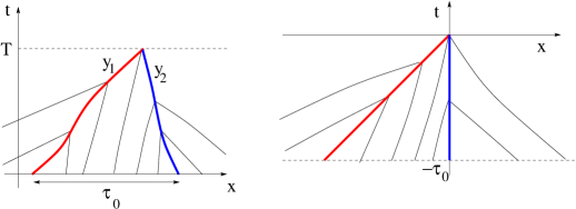
Figure 3: Positions of the two shocks in the original variables (left), and in the adapted variables (right).

We shall construct the solution of (6.5) in the form

$$u(t,x)~{}=~{}w(t,x)+\varphi(t,x)\qquad\hbox{for all}~{}(t,x)\in[\tau_{0},0]\,\times\mathbb{R}\,.$$ (6.7)

Here $\varphi$ is a continuous function, which satisfies $\varphi(t,t)=\varphi(t,0)=0$, while

$$w(t,\cdot)~{}\in~{}H^{2}\Big{(}]-\infty,t[~{}\cup~{}]t,0[~{}\cup~{}]0,+\infty[\Big{)}\qquad\hbox{for all}~{}t\in[\tau_{0},0].$$ (6.8)

According to (6.8), the function $w(t,\cdot)$ is continuously differentiable outside the two points $x=t$ and $x=0$. Moreover, the distributional derivative $D_{x}w(t,\cdot)$ is an ${\bf L}^{2}$ function restricted to each interval $]-\infty,t[\,$, $]t,0[\,$ and $]0,+\infty[\,$. However, both $w(t,\cdot)$ and $w_{x}(t,\cdot)$ can have a jump at $x=t$ and at $x=0$. At the points $(t,t)$ and $(t,0)$, the following traces are well defined:

$$\left\{\begin{array}[]{cl}w^{-}_{1}(t)~{}\doteq~{}w(t,t-)~{}=~{}u^{-}_{1}(t),\cr\cr w^{+}_{1}(t)~{}\doteq~{}w(t,t+)~{}=~{}u^{+}_{1}(t),\end{array}\right.\qquad\qquad\qquad\qquad\left\{\begin{array}[]{cl}b^{-}_{1}(t)~{}\doteq~{}w_{x}(t,t-),\cr\cr b^{+}_{1}(t)~{}\doteq~{}w_{x}(t,t+),\end{array}\right.$$ (6.9)

$$\left\{\begin{array}[]{cl}w^{-}_{2}(t)~{}\doteq~{}w(t,0-)~{}=~{}u^{-}_{2}(t),\cr\cr w^{+}_{2}(t)~{}\doteq~{}w(t,0+)~{}=~{}u^{+}_{2}(t),\end{array}\right.\qquad\qquad\qquad\qquad\left\{\begin{array}[]{cl}b^{-}_{2}(t)~{}\doteq~{}w_{x}(t,0-),\cr\cr b^{+}_{2}(t)~{}\doteq~{}w_{x}(t,0+).\end{array}\right.$$ (6.10)

For the shocks to be entropy admissible, the inequalities

$$w_{1}^{-}(t)~{}>~{}w_{1}^{+}(t),\qquad\qquad w_{2}^{-}(t)~{}>~{}w_{2}^{+}(t),$$ (6.11)

will always be assumed. Writing

$$a^{(w)}_{1}(t)~{}\doteq~{}{w^{-}_{1}(t)+w^{+}_{1}(t)\over 2}\qquad\qquad a^{(w)}_{2}(t)~{}\doteq~{}{w^{-}_{2}(t)+w^{+}_{2}(t)\over 2}\,,$$ (6.12)

the equation (6.5) reads

$$w_{t}+a(t,x,w)\cdot w_{x}~{}=~{}F(t,x,w),$$ (6.13)

where $a$ and $F$ are given by

$$a(t,x,w)~{}=~{}{w(t,x)+\varphi^{(w)}(t,x)-a^{(w)}_{2}(t)\over a^{(w)}_{1}(t)-a^{(w)}_{2}(t)}\,,$$ (6.14)

$$F(t,x,w)~{}=~{}\left[{{\bf H}[w]-(w-a^{(w)}_{2}(t))\cdot\varphi^{(w)}_{x}\over a^{(w)}_{1}(t)-a^{(w)}_{2}(t)}-\varphi^{(w)}_{t}\right]+{{\bf H}[\varphi^{(w)}]-\varphi^{(w)}\varphi^{(w)}_{x}\over a^{(w)}_{1}(t)-a^{(w)}_{2}(t)},$$ (6.15)

respectively. Here the function $\varphi^{(w)}(t,x)$ is chosen in such a way that a cancellation between leading order terms near to the location of the two shocks at $x=t$ and at $x=0$ is achieved. More precisely, in view of (5.14) and recalling (2.3) and (2.4), we set

$$\phi_{0}(x)~{}=~{}\phi(x,0)~{}=~{}{2\eta(x)\over\pi}\cdot|x|\ln|x|,$$ (6.16)

and define

$$\varphi^{(w)}(t,x)\,=\,\left\{\begin{array}[]{cl}\displaystyle\phi_{0}(x-t)+{\sigma^{(w)}_{2}(t)\over 2\sigma^{(w)}_{1}(t)+\sigma^{(w)}_{2}(t)}\cdot\big{(}\phi_{0}(x)-\phi_{0}(t)\big{)}&\hbox{if}~{}~{}x<t,\\[17.07164pt] \displaystyle\phi_{0}(x-t)+\phi_{0}(x)-\phi_{0}(t)&\hbox{if}~{}~{}t<x<0,\\[8.53581pt] \displaystyle{\sigma^{(w)}_{1}(t)\over\sigma^{(w)}_{1}(t)+2\sigma^{(w)}_{2}(t)}\cdot\big{(}\phi_{0}(x-t)-\phi_{0}(t)\big{)}+\phi_{0}(x)&\hbox{if}~{}~{}0<x\,.\end{array}\right.$$ (6.17)

The following theorem provides the existence of solutions to the Cauchy problem for (1.1) where the initial datum contains two shocks. In particular, the solution to (6.5) is constructed up to the time where the two shocks interact. Furthermore, the solution is of the form (6.7), where $\varphi=\varphi^{(w)}$, the corrector function defined in (6.17).

Theorem 6.1

For any given constants $b$, $M_{0}$, $\delta_{1}$, $\delta_{2}>0$, there exists $\varepsilon_{0}>0$ small enough and a constant $K$ such that the following holds.

Consider any $\tau_{0}\in[-\varepsilon_{0},0[\,$ and any initial condition $\overline{w}\in H^{2}(\mathbb{R}\backslash\{\tau_{0},0\})$ such that

$$\left\{\begin{array}[]{rll}\|\overline{w}\|_{H^{2}(\mathbb{R}\backslash\{\tau_{0},0\})}&\leq~{}\displaystyle{M_{0}\over 4},&\left\|\overline{w}_{x}\right\|_{{\bf L}^{\infty}(]\tau_{0},0[)}~{}\leq~{}b,\\[11.38109pt] \overline{w}(\tau_{0}-)-\overline{w}(\tau_{0}+)&\geq~{}8\delta_{1},&\overline{w}(0-)-\overline{w}(0+)~{}\geq~{}8\delta_{2}.\end{array}\right.$$ (6.18)

Then the Cauchy problem (6.13) with initial data

$$w(\tau_{0},\cdot)~{}=~{}\overline{w}~{}\in~{}H^{2}\bigl{(}\mathbb{R}\setminus\{\tau_{0},0\}\bigr{)}$$ (6.19)

admits a unique entropic solution, defined for $t\in[\tau_{0},0]$. Moreover, this solution satisfies

$$\left\{\begin{array}[]{rll}\|w(t,\cdot)\|_{H^{2}(\mathbb{R}\backslash\{t,0\})}&\leq~{}M_{0},&\left\|w_{x}(t,\cdot)\right\|_{{\bf L}^{\infty}(]\tau_{0},0[)}~{}\leq~{}Kb,\\[11.38109pt] w(t,t-)-w(t,t+)&\geq~{}\delta_{1},&w(t,0-)-w(t,0+)~{}\geq~{}\delta_{2}\end{array}\right.$$ (6.20)

for all $t\in[\tau_{0},0[$.

Remark 6.1

By (6.20), at the interaction time $t=0$ the solution $u=w+\varphi^{(w)}$ is the sum of a corrector term plus a function in $H^{2}\bigl{(}\mathbb{R}\setminus\{0\}\bigr{)}$. This function lies within the class of initial data covered by our earlier Theorem 2.1. Thus, combining Theorems 6.1 and 2.1 yields the behavior of a solution to (1.1) across the interaction of two shocks.

Toward a proof of Theorem 6.1, solutions to (6.13) will be constructed by an iteration procedure. The main difference between this and the earlier case with a single shock is that the correction term $\varphi$ now depends on time through the variable strengths $\sigma_{1},\sigma_{2}$ of the two shocks. Define

$$w^{(1)}(t,x)~{}=~{}\begin{cases}\overline{w}(x)&\qquad\mathrm{if}~{}~{}x\in]t,0[\cup]0,\infty[,\\[5.69054pt] \overline{w}(x+\tau_{0}-t)&\qquad\mathrm{if}~{}~{}x\in]-\infty,t[.\end{cases}$$ (6.21)

By induction, let $w^{(n)}$ be given and satisfy (6.8) for every $t\in[\tau_{0},0[\,$. Moreover, call $\sigma_{1}^{(n)}(t)$ and $\sigma_{2}^{(n)}(t)$ the strengths of the two shocks at $x=t$ and $x=0$ of $w^{(n)}$, respectively. We construct the next iterate $w=w^{(n+1)}(t,x)$ by solving the linear equation

$$w_{t}+a\left(t,x,w^{(n)}\right)\,w_{x}~{}=~{}F(t,x,w),$$ (6.22)

with initial data (6.19) and $a$ as introduced in (6.14).

The induction argument requires the following steps:

• Given $w^{(n)}$, the equation (6.22) with the initial data $\overline{w}$ admits a unique solution $w$ with $w(t,\cdot)\in H^{2}\bigl{(}\mathbb{R}\setminus\{t,0\}\bigr{)}$ for all $t\in[\tau_{0},0[\,$.

• A priori bounds on the strong norm $\|w^{(n)}(t,\cdot)\|_{H^{2}\bigl{(}\mathbb{R}\setminus\{t,0\}\bigr{)}}$ for all $t\in[\tau_{0},0[$, $n\geq 1$.

• Convergence in a weak norm. This will follow from the bound

  $$\sum_{n\geq 1}\|w^{(n+1)}(t,\cdot)-w^{(n)}(t,\cdot)\|_{H^{2}\bigl{(}\mathbb{R}\setminus\{t,0\}\bigr{)}}~{}<~{}+\infty.$$

6.1 Some preliminary estimates

To achieve the above steps (i)-(iii), we first establish some key estimates on the right hand side of (6.13). For any $w:[\tau_{0},0]\times\mathbb{R}\to\mathbb{R}$ such that $w(t,\cdot)\in H^{2}(\mathbb{R}\backslash\{t,0\})$ for all $t\in[\tau_{0},0]$, we write

$$w(t,\cdot)~{}=~{}v_{1}(t,\cdot)+v_{2}(t,\cdot)$$ (6.23)

with

$$v_{2}(t,x)~{}\doteq~{}\begin{cases}\left(w(t,0-)+x\cdot w_{x}(t,0-)\right)\cdot\eta(x)&\mathrm{if}~{}~{}~{}x<0\,,\\[8.53581pt] \left(w(t,0+)+x\cdot w_{x}(t,0+)\right)\cdot\eta(x)&\mathrm{if}~{}~{}~{}x>0.\end{cases}$$ (6.24)

Recalling (6.9)-(6.12) and (6.15), we split $F$ into the four parts:

$$F(t,x,w)~{}=~{}\displaystyle{1\over a^{(w)}_{1}(t)-a^{(w)}_{2}(t)}\cdot\Big{[}{A^{(w)}(t,x)+B^{(w)}(t,x)+C^{(w)}(t,x)+D^{(w)}(t,x)}\Big{]}.$$ (6.25)

Here we take

$$A^{(w)}~{}\doteq~{}{\bf H}\left[\varphi^{(w)}\right]-\varphi^{(w)}\varphi_{x}^{(w)},\quad B^{(w)}~{}=~{}\widetilde{B}^{(v_{2})}~{}\doteq~{}{\bf H}[v_{2}]-\left(v_{2}-{v_{2}(t,0-)+v_{2}(t,0+)\over 2}\right)\cdot\phi^{\prime}_{0}(x)\,,$$ (6.26)

$$C^{(w)}~{}=~{}\widetilde{C}^{(v_{1})}~{}\doteq~{}{\bf H}[v_{1}]-\left(v_{1}-{v_{1}(t,t-)+v_{1}(t,t+)\over 2}\right)\cdot\phi^{\prime}_{0}(x-t),$$ (6.27)

$$D^{(w)}~{}\doteq~{}{\bf H}[w]-\left(w-a^{(w)}_{2}(t)\right)\cdot\varphi^{(w)}_{x}-\left(a^{(w)}_{1}(t)-a^{(w)}_{2}(t)\right)\cdot\varphi^{(w)}_{t}-B^{(w)}-C^{(w)}.$$ (6.28)

Lemma 6.1

Let $w:[\tau_{0},0]\times\mathbb{R}\to\mathbb{R}$ be such that $w(t,\cdot)\in H^{2}(\mathbb{R}\backslash\{t,0\})$ for all $t\in[\tau_{0},0]$, and

$$\|w(t,\cdot)\|_{H^{2}(\mathbb{R}\backslash\{t,0\})}~{}\leq~{}M_{0},\qquad|w_{x}(t,0-)|+|w_{x}(t,0+)|~{}\leq~{}b,\qquad\sigma_{j}^{(w)}(t)~{}\geq~{}\delta_{0}~{}>~{}0.$$

Moreover, assume that $\displaystyle-{1\over 4}\cdot\min\left\{1,{\delta^{2}_{0}\over M_{0}^{2}}\right\}<\tau_{0}<0$ and $\sigma_{j}^{(w)}(\cdot)$ is locally Lipschitz on $[\tau_{0},0[$ for $j=1,2$. Then there is a constant $C_{1}>0$, depending only on $M_{0}$, $b$, $\delta_{0}$ such that, for a.e. $t\in[\tau_{0},0]$ and $|x|<{1\over 2e}$, one has

$$\begin{cases}|F(t,x,w)|~{}\leq~{}C_{1}\cdot\Bigg{[}\displaystyle{1+M_{0}+b\over\delta_{0}}+\big{|}\ln|t|\big{|}\\ \qquad\qquad\qquad\qquad\qquad\qquad\qquad\displaystyle+~{}\chi_{\mathbb{R}^{\backslash}]t,0[}\cdot{\left|\dot{\sigma}_{1}^{(w)}(t)\right|+\left|\dot{\sigma}_{2}^{(w)}(t)\right|\over\delta_{0}}\cdot\left(|x|^{1/2}+|x-t|^{1/2}\right)\Bigg{]},\\[11.38109pt] |F_{x}(t,x,w)|~{}\leq~{}C_{1}\cdot\displaystyle{1+M_{0}+b+\chi_{\mathbb{R}^{\backslash}]t,0[}\cdot\left(\left|\dot{\sigma}_{1}^{(w)}(t)\right|+\left|\dot{\sigma}_{2}^{(w)}(t)\right|\right)\over\delta_{0}}\cdot\left(|x|^{-1/2}+|x-t|^{-1/2}\right).\end{cases}$$ (6.29)

Furthermore, for every $\delta>0$ sufficiently small one has for all $t\in[\tau_{0},0]$

$$\|F(t,x,w)\|_{H^{2}(\mathbb{R}\backslash[-\delta,\delta]\cup[t-\delta,t+\delta])}~{}\leq~{}\displaystyle C_{1}\cdot\left[{1+M_{0}+b+\left|\dot{\sigma}_{1}^{(w)}(t)\right|+\left|\dot{\sigma}_{2}^{(w)}(t)\right|\over\delta_{0}}\cdot\displaystyle\delta^{-2/3}+|\ln(t)|\right].$$ (6.30)

Proof. We observe that, for all $t\in[\tau_{0},0]$, it holds

$$a_{1}^{(w)}(t)-a_{2}^{(w)}(t)~{}\geq~{}\delta_{0}+w(t,t+)-w(t,0-)~{}\geq~{}\delta_{0}-M_{0}\cdot|t|^{1/2}~{}\geq~{}{\delta_{0}\over 2},$$ (6.31)

$$0<\sigma^{(w)}_{j}(t)<\sigma_{1}^{(w)}(t)+\sigma_{2}^{(w)}(t)=w(t,t-)-w(t,t+)+w(t,0-)-w(t,0+)\leq(2+\sqrt{|t|})M_{0},$$

$$\|v_{1}(t,\cdot)\|_{H^{2}(\mathbb{R}\backslash\{t\})},\|v_{2}(t,\cdot)\|_{H^{2}(\mathbb{R}\backslash\{0\})}~{}\leq~{}{\cal O}(1)\cdot(M_{0}+b).$$

According to (6.25), the function $F$ can be decomposed as the sum of four terms, which will be estimated separately.

1. Recalling (3.2) and (3.10), (6.26) and (6.27) imply that for every $(t,x)\in[\tau_{0},0]\times\left[-{1\over 2e},{1\over 2e}\right]$ one has

$$\begin{cases}\left|B^{(w)}(t,x)\right|~{}\leq~{}{\cal O}(1)\cdot(M_{0}+b),\qquad\left|B^{(w)}_{x}(t,x)\right|~{}\leq~{}{\cal O}(1)\cdot(M_{0}+b)\cdot\big{|}\ln|x|\big{|}^{2},\\[8.53581pt] \left\|B^{(w)}(t,\cdot)\right\|_{H^{2}(\mathbb{R}\backslash[-\delta,\delta])}~{}\leq~{}{\cal O}(1)\cdot(M_{0}+b)\cdot\delta^{-2/3}.\end{cases}$$ (6.32)

and, for every $(t,x)\in[\tau_{0},0]\times\left[t-{1\over 2e},t+{1\over 2e}\right]$

$$\begin{cases}\left|C^{(w)}(t,x)\right|~{}\leq~{}{\cal O}(1)\cdot(M_{0}+b),\qquad\left|C^{(w)}_{x}(t,x)\right|~{}\leq~{}{\cal O}(1)\cdot(M_{0}+b)\cdot\big{|}\ln|x-t|\big{|}^{2},\\[8.53581pt] \left\|C^{(w)}(t,\cdot)\right\|_{H^{2}(\mathbb{R}\backslash[t-\delta,t+\delta])}~{}\leq~{}{\cal O}(1)\cdot(M_{0}+b)\cdot\delta^{-2/3}.\end{cases}$$ (6.33)

2. Next, we estimate $A^{(w)}$. Recalling (3.4), i.e.,

$$g_{b}(x)~{}=~{}\chi_{[0,\infty[}(x)\cdot\phi(x,b),\qquad x\in\mathbb{R},b\geq 0,$$

(2.4), and (6.16), we can rewrite, for $(t,x)\in[\tau_{0},0]\times\left[-{1\over 2e},{1\over 2e}\right]$,

$$\varphi^{(w)}(t,x)~{}=~{}\phi_{0}(x-t)+\phi_{0}(x)-\phi_{0}(t)+E_{1}^{(w)}(t,x)+E_{2}^{(w)}(t,x),$$ (6.34)

$$\begin{cases}E_{1}^{(w)}(t,x)&=~{}-\displaystyle{2\cdot\chi_{]-\infty,t]}\cdot\sigma^{(w)}_{1}(t)\over 2\sigma^{(w)}_{1}(t)+\sigma^{(w)}_{2}(t)}\cdot\big{[}\phi_{0}(x)-\phi_{0}(t)\big{]}~{}=~{}\displaystyle-{2\sigma^{(w)}_{1}(t)\over 2\sigma^{(w)}_{1}(t)+\sigma^{(w)}_{2}(t)}\cdot g_{|t|}(t-x),\\[11.38109pt] E_{2}^{(w)}(t,x)&=~{}-\displaystyle{2\cdot\chi_{[0,\infty[}\cdot\sigma^{(w)}_{2}(t)\over\sigma^{(w)}_{1}(t)+2\sigma^{(w)}_{2}(t)}\cdot\big{[}\phi_{0}(x-t)-\phi_{0}(t)\big{]}~{}=~{}-{2\sigma^{(w)}_{2}(t)\over\sigma^{(w)}_{1}(t)+2\sigma^{(w)}_{2}(t)}\cdot g_{|t|}(x).\end{cases}$$ (6.35)

Thus, for $(t,x)\in[\tau_{0},0]\times\left[-{1\over 2e},{1\over 2e}\right]$, Lemma 3.1 and [4, Section 3] imply,

$$\left\{\begin{array}[]{rlrl}&\big{|}{\bf H}\big{[}\varphi^{(w)}(t,\cdot)\big{]}(x)\big{|}\displaystyle~{}\leq~{}\displaystyle{\cal O}(1),\quad\displaystyle\left|{d\over dx}{\bf H}\big{[}\varphi^{(w)}(t,\cdot)\big{]}(x)\right|\displaystyle\leq~{}{\cal O}(1)\cdot\left(\ln^{2}|x|+\ln^{2}|x-t|\right),\\[11.38109pt] &\big{\|}{\bf H}\big{[}\varphi^{(w)}(t,\cdot)\big{]}\big{\|}_{H^{2}(\mathbb{R}\backslash([-\delta,\delta])\cup[t-\delta,t+\delta])}~{}\leq~{}{\cal O}(1)\cdot\delta^{-2/3}.\end{array}\right.$$ (6.36)

On the other hand, given $t\in[\tau_{0},0]$, for every $|x|\leq\frac{1}{2e}$, (6.34) combined with (3.5) yields

$$\left|\varphi^{(w)}(t,x)\right|\leq\min(|x\ln(|x|)|,|(x-t)\ln(|x-t|)|).$$

Furthermore, we compute for every $x\in\mathbb{R}\backslash\{t,0\}$

$$\varphi_{x}^{(w)}(t,x)~{}=~{}~{}\left(1-\displaystyle{2\cdot\chi_{[0,\infty[}\cdot\sigma^{(w)}_{2}(t)\over\sigma^{(w)}_{1}(t)+2\sigma^{(w)}_{2}(t)}\right)\phi^{\prime}_{0}(x-t)+\left(1-\displaystyle{2\cdot\chi_{]-\infty,t]}\cdot\sigma^{(w)}_{1}(t)\over 2\sigma^{(w)}_{1}(t)+\sigma^{(w)}_{2}(t)}\right)\cdot\phi^{\prime}_{0}(x),$$ (6.37)

which together with [4, Section 3] implies for $|x|\leq\frac{1}{2e}$ that

$$\left|\varphi_{x}^{(w)}(t,x)\right|~{}\leq~{}{\cal O}(1)\cdot\left(\big{|}\ln|x|\big{|}+\big{|}\ln|x-t|\big{|}\right),\qquad\left|\varphi_{xx}^{(w)}(t,x)\right|~{}\leq~{}{\cal O}(1)\cdot\left({1\over|x|}+{1\over|x-t|}\right),$$

$$\left|\varphi_{xxx}^{(w)}(t,x)\right|~{}\leq~{}{\cal O}(1)\cdot\left({1\over x^{2}}+{1\over(x-t)^{2}}\right).$$

A direct computation yields, for $|x|\leq\frac{1}{2e}$,

$$\begin{cases}\left|\varphi^{(w)}\varphi_{x}^{(w)}(t,x)\right|&\leq~{}{\cal O}(1)\cdot\left(|x|^{1/2}+|x-t|^{1/2}\right),\\[5.69054pt] \left|\displaystyle{d\over dx}[\varphi^{(w)}\varphi_{x}^{(w)}](t,x)\right|&\leq~{}{\cal O}(1)\cdot\left(\ln^{2}|x|+\ln^{2}|x-t|\right),\\[8.53581pt] \left|\displaystyle{d^{2}\over dx^{2}}[\varphi^{(w)}\varphi_{x}^{(w)}](t,x)\right|&\leq~{}{\cal O}(1)\cdot\displaystyle\left(\left|{\ln|x|\over x}\right|+\left|{\ln|x-t|\over x-t}\right|\right).\end{cases}$$

and thus

$$\left\|\varphi^{(w)}\varphi_{x}^{(w)}(t,\cdot)\right\|_{H^{2}(\mathbb{R}\backslash[t-\delta,t+\delta]\cup[-\delta,\delta])}~{}\leq~{}{\cal O}(1)\cdot\delta^{-2/3}.$$

Recalling (6.36), we get

$$\begin{cases}\left|A^{(w)}(t,x)\right|~{}\leq~{}{\cal O}(1),\qquad\left|A^{(w)}_{x}(t,x)\right|~{}\leq~{}{\cal O}(1)\cdot\left(\ln^{2}|x|+\ln^{2}|x-t|\right),\\[5.69054pt] \left\|A^{(w)}(t,\cdot)\right\|_{H^{2}(\mathbb{R}\backslash[t-\delta,t+\delta]\cup(-\delta,\delta))}~{}\leq~{}{\cal O}(1)\cdot\delta^{-2/3}.\end{cases}$$ (6.38)

3. Finally, to estimate $D^{(w)}$, we shall consider three cases:

Case 1: Assume that $-{1\over 2}<t-{1\over 2e}<x<t$. We have

$$D^{(w)}(t,x)~{}=~{}D^{(w)}_{1}(t,x)+D^{(w)}_{2}(t,x)+D_{3}^{(w)}(t,x)$$ (6.39)

with

$$\begin{cases}D_{1}^{(w)}(t,x)~{}=~{}w_{x}(t,0-)\cdot(t-x)\cdot\phi_{0}^{\prime}(x-t),\\[5.69054pt] D_{2}^{(w)}(t,x)~{}=~{}\displaystyle\displaystyle\left({\sigma^{(w)}_{2}(t)\cdot[w(t,0-)-w(t,t+)+w(t,t-)-w(t,x)]\over 2\sigma^{(w)}_{1}(t)+\sigma^{(w)}_{2}(t)}+xw_{x}(t,0-)\right)\cdot\phi^{\prime}_{0}(x),\\[11.38109pt] D_{3}^{(w)}(t,x)~{}=~{}\big{[}a^{(w)}_{2}(t)-a^{(w)}_{1}(t)\big{]}\cdot\left[\left(\displaystyle{\sigma^{(w)}_{2}(t)\over 2\sigma^{(w)}_{1}(t)+\sigma^{(w)}_{2}(t)}\right)^{\prime}\cdot g_{|t|}(t-x)-\displaystyle{\sigma^{(w)}_{2}(t)\cdot\phi^{\prime}_{0}(t)\over 2\sigma^{(w)}_{1}(t)+\sigma^{(w)}_{2}(t)}\right].\end{cases}$$

Recalling (6.16), we estimate

$$\begin{cases}\left|D_{1}^{(w)}(t,x)\right|~{}\leq~{}{\cal O}(1)\cdot b\cdot|x-t|\big{|}\ln|x-t|\big{|}~{}\leq~{}O(1)\cdot b,\\[5.69054pt] \left|\displaystyle{d\over dx}D_{1}^{(w)}(t,x)\right|~{}\leq~{}{\cal O}(1)\cdot b\cdot\big{|}\ln|x-t|\big{|},\qquad\left|\displaystyle{d^{2}\over d^{2}x}D_{1}^{(w)}(t,x)\right|~{}\leq~{}\displaystyle O(1)\cdot{b\over|x-t|},\end{cases}$$ (6.40)

$$\begin{cases}\left|D_{2}^{(w)}(t,x)\right|~{}\leq~{}{\cal O}(1)\cdot(M_{0}+b)\cdot x\big{|}\ln|x|\big{|},\quad\left|\displaystyle{d\over dx}D_{2}^{(w)}(t,x)\right|~{}\leq~{}{\cal O}(1)\cdot(M_{0}+b)\cdot\big{|}\ln|x|\big{|},\\[8.53581pt] \left|\displaystyle{d^{2}\over dx^{2}}D_{2}^{(w)}(t,x)\right|~{}\leq~{}\displaystyle|w_{xx}\cdot\phi^{\prime}_{0}(x)|+{\cal O}(1)\cdot{M_{0}+b\over|x|},\end{cases}$$ (6.41)

and

$$\begin{cases}\left|D_{3}^{(w)}(t,x)\right|~{}\leq~{}\displaystyle{\cal O}(1)\cdot\left|a^{(w)}_{2}(t)-a^{(w)}_{1}(t)\right|\cdot\left({\left|\dot{\sigma}^{(w)}_{1}(t)\right|+\left|\dot{\sigma}^{(w)}_{2}(t)\right|\over\delta_{0}}|x-t||\ln|x-t||+\big{|}\ln|t|\big{|}\right)\\[11.38109pt] \left|\displaystyle{d\over dx}D_{3}^{(w)}(t,x)\right|~{}\leq~{}\displaystyle{\cal O}(1)\cdot\left|a^{(w)}_{2}(t)-a^{(w)}_{1}(t)\right|\cdot{\left|\dot{\sigma}^{(w)}_{1}(t)\right|+\left|\dot{\sigma}^{(w)}_{2}(t)\right|\over\delta_{0}}\cdot\big{|}\ln|x-t|\big{|},\\[11.38109pt] \left|\displaystyle{d^{2}\over dx^{2}}D_{3}^{(w)}(t,x)\right|~{}\leq~{}\displaystyle{\cal O}(1)\cdot\left|a^{(w)}_{2}(t)-a^{(w)}_{1}(t)\right|\cdot{\left|\dot{\sigma}^{(w)}_{1}(t)\right|+\left|\dot{\sigma}^{(w)}_{2}(t)\right|\over\delta_{0}}\cdot{1\over|x-t|}\,.\end{cases}$$ (6.42)

Combining (6.39)-(6.42), we obtain

$$\begin{cases}\displaystyle{\left|D^{(w)}(t,x)\right|\over\left|a^{(w)}_{2}(t)-a^{(w)}_{1}(t)\right|}~{}\leq~{}{\cal O}(1)\cdot\left({M_{0}+b\over\delta_{0}}+|\ln(t)|+{\left|\dot{\sigma}^{(w)}_{1}(t)\right|+\left|\dot{\sigma}^{(w)}_{2}(t)\right|\over\delta_{0}}\cdot|x-t|^{1/2}\right),\\[11.38109pt] \displaystyle{\left|\displaystyle{d\over dx}D^{(w)}(t,x)\right|\over\left|a^{(w)}_{2}(t)-a^{(w)}_{1}(t)\right|}~{}\leq~{}\displaystyle{\cal O}(1)\cdot{M_{0}+b+\left|\dot{\sigma}^{(w)}_{1}(t)\right|+\left|\dot{\sigma}^{(w)}_{2}(t)\right|\over\delta_{0}}\cdot\big{|}\ln|x-t|\big{|},\\[11.38109pt] \displaystyle{\left|\displaystyle{d^{2}\over dx^{2}}D^{(w)}(t,x)\right|\over\left|a^{(w)}_{2}(t)-a^{(w)}_{1}(t)\right|}~{}\leq~{}\displaystyle{\cal O}(1)\cdot\left({M_{0}+b+\left|\dot{\sigma}^{(w)}_{1}(t)\right|+\left|\dot{\sigma}^{(w)}_{2}(t)\right|\over\delta_{0}\cdot|x-t|}+{|w_{xx}|\over\delta_{0}}\cdot\big{|}\ln|x-t|\big{|}\right).\end{cases}$$ (6.43)

Case 2: Assume that $\displaystyle t<x<0$. We have

$$D^{(w)}(t,x)~{}=~{}w_{x}(t,0-)\cdot(t-x)\cdot\phi_{0}^{\prime}(x-t)+(v_{1}(t,0)-v_{1}(t,x))\cdot\phi^{\prime}_{0}(x)+\big{[}a^{(w)}_{1}(t)-a^{(w)}_{2}(t)\big{]}\cdot\phi_{0}^{\prime}(t),$$ (6.44)

and this yields

$$\begin{cases}\displaystyle{\left|D^{(w)}(t,x)\right|\over\left|a^{(w)}_{2}(t)-a^{(w)}_{1}(t)\right|}~{}\leq~{}{\cal O}(1)\left({M_{0}+b\over\delta_{0}}+\big{|}\ln|t|\big{|}\right),\\[11.38109pt] \displaystyle{\left|\displaystyle{d\over dx}D^{(w)}(t,x)\right|\over\left|a^{(w)}_{2}(t)-a^{(w)}_{1}(t)\right|}~{}\leq~{}{\cal O}(1)\cdot{M_{0}+b\over\delta_{0}}\cdot\left(\big{|}\ln|x|\big{|}+\big{|}\ln|x-t|\big{|}\right),\\[11.38109pt] \displaystyle{\left|\displaystyle{d^{2}\over dx^{2}}D^{(w)}(t,x)\right|\over\left|a^{(w)}_{2}(t)-a^{(w)}_{1}(t)\right|}~{}\leq~{}\displaystyle{\cal O}(1)\cdot\left({M_{0}+b\over\delta_{0}}\cdot\left({1\over|x|}+{1\over|x-t|}\right)+{\big{|}w_{xx}(t,x)|\over\delta_{0}}\cdot\big{|}\ln|x|\big{|}\right).\end{cases}$$ (6.45)

Case 3: Assume that $0<x<1/2$. As in Case 1, writing

$$D^{(w)}(t,x)~{}=~{}D^{(w)}_{1}(t,x)+D^{(w)}_{2}(t,x)+D_{3}^{(w)}(t,x)$$ (6.46)

with

$$\begin{cases}D_{1}^{(w)}(t,x)~{}=~{}\left[v_{1}(t,x)-v_{1}(t,t+)\right]\cdot\phi_{0}^{\prime}(x-t)\\ \qquad\qquad+~{}\left[\displaystyle{\sigma^{(w)}_{1}(t)\over\sigma^{(w)}_{1}(t)+2\sigma^{(w)}_{2}(t)}\cdot(w(t,t+)-w(t,0-)+w(t,0+)-w(t,x))\right]\cdot\phi_{0}^{\prime}(x-t),\\[11.38109pt] D_{2}^{(w)}(t,x)~{}=~{}\displaystyle\displaystyle\left(w(t,0+)-w(t,x)+xw_{x}(t,0+)\right)\cdot\phi^{\prime}_{0}(x),\\[11.38109pt] D_{3}^{(w)}(t,x)~{}=~{}\big{[}a^{(w)}_{2}(t)-a^{(w)}_{1}(t)\big{]}\cdot\left[\left(\displaystyle{\sigma^{(w)}_{1}(t)\over\sigma^{(w)}_{1}(t)+2\sigma^{(w)}_{2}(t)}\right)^{\prime}\cdot g_{|t|}(x)-\displaystyle{\sigma^{(w)}_{1}(t)\cdot\phi^{\prime}_{0}(t)\over\sigma^{(w)}_{1}(t)+2\sigma^{(w)}_{2}(t)}\right],\end{cases}$$

we estimate

$$\begin{cases}\displaystyle{\left|D^{(w)}(t,x)\right|\over\left|a^{(w)}_{2}(t)-a^{(w)}_{1}(t)\right|}~{}\leq~{}\displaystyle{\cal O}(1)\cdot\left({M_{0}+b\over\delta_{0}}+|\ln(t)|+{\left|\dot{\sigma}^{(w)}_{1}(t)\right|+\left|\dot{\sigma}^{(w)}_{2}(t)\right|\over\delta_{0}}\cdot|x|^{1/2}\right),\\[11.38109pt] \displaystyle{\left|\displaystyle{d\over dx}D^{(w)}(t,x)\right|\over\left|a^{(w)}_{2}(t)-a^{(w)}_{1}(t)\right|}~{}\leq~{}\displaystyle{\cal O}(1)\cdot{M_{0}+b+\left|\dot{\sigma}^{(w)}_{1}(t)\right|+\left|\dot{\sigma}^{(w)}_{2}(t)\right|\over\delta_{0}}\cdot\big{|}\ln|x|\big{|},\\[11.38109pt] \displaystyle{\left|\displaystyle{d^{2}\over dx^{2}}D^{(w)}(t,x)\right|\over\left|a^{(w)}_{2}(t)-a^{(w)}_{1}(t)\right|}~{}\leq~{}\displaystyle{\cal O}(1)\cdot\left({M_{0}+b+\left|\dot{\sigma}^{(w)}_{1}(t)\right|+\left|\dot{\sigma}^{(w)}_{2}(t)\right|\over\delta_{0}}\cdot{1\over|x|}+{|w_{xx}|\over\delta_{0}}\cdot\big{|}\ln|x|\big{|}\right).\end{cases}$$ (6.47)

In summary, from (6.43), (6.45), and (6.47), given $t\in[\tau_{0},0]$, for every $x\in(-1/2,1/2)\backslash\{t,0\}$, it holds that

$$\begin{cases}\displaystyle{\left|D^{(w)}(t,x)\right|\over\left|a^{(w)}_{2}(t)-a^{(w)}_{1}(t)\right|}~{}\leq~{}{\cal O}(1)\cdot\Bigg{(}{M_{0}+b\over\delta_{0}}+|\ln(t)|\\ \qquad\qquad\qquad\qquad\qquad\qquad\qquad\quad\displaystyle+\chi_{\mathbb{R}\backslash]0,t[}\cdot{\left|\dot{\sigma}^{(w)}_{1}(t)\right|+\left|\dot{\sigma}^{(w)}_{2}(t)\right|\over\delta_{0}}\cdot\left(|x|^{1/2}+|x-t|^{1/2}\right)\Bigg{)},\\[11.38109pt] \displaystyle{\left|\displaystyle{d\over dx}D^{(w)}(t,x)\right|\over\left|a^{(w)}_{2}(t)-a^{(w)}_{1}(t)\right|}\leq{\cal O}(1)\cdot{M_{0}+b+\chi_{\mathbb{R}\backslash]t,0[}\left(\left|\dot{\sigma}^{(w)}_{1}(t)\right|+\left|\dot{\sigma}^{(w)}_{2}(t)\right|\right)\over\delta_{0}}\cdot\left(\big{|}\ln|x|\big{|}+\big{|}\ln|x-t|\big{|}\right),\\[11.38109pt] \displaystyle{\left\|D^{(w)}(t,\cdot)\right\|_{H^{2}(\mathbb{R}\backslash[t-\delta,t+\delta]\cup(-\delta,\delta))}\over\left|a^{(w)}_{2}(t)-a^{(w)}_{1}(t)\right|}~{}\leq~{}\displaystyle{\cal O}(1)\cdot\left[{M_{0}+b+\left|\dot{\sigma}^{(w)}_{1}(t)\right|+\left|\dot{\sigma}^{(w)}_{2}(t)\right|\over\delta_{0}\delta^{2/3}}+\big{|}\ln|t|\big{|}\right].\end{cases}$$ (6.48)

To complete the proof, combining (6.32), (6.33), (6.38) and (6.48), we obtain (6.29)-(6.30). MM     

The next lemma estimates the change in the function $F=F(t,x,w)$ as $w(\cdot)$ takes different values. These estimates will play a key role in the proof of convergence of the approximations inductively defined by (6.22).

Lemma 6.2

Let $w_{1},w_{2}:[\tau_{0},0]\times\mathbb{R}\to\mathbb{R}$ be such that, for $i\in\{1,2\}$ and $t\in[\tau_{0},0]$, one has $w_{i}(t,\cdot)\in H^{2}(\mathbb{R}\backslash\{t,0\})$ and

$$\|w_{i}(t,\cdot)\|_{H^{2}(\mathbb{R}\backslash\{t,0\})}~{}\leq~{}M_{0},\qquad|w_{i,x}(t,0-)|+|w_{i,x}(t,0+)|~{}\leq~{}b,\qquad\left|\sigma_{j}^{(w_{i})}(t)\right|~{}\geq~{}\delta_{0}.$$

Moreover, assume that $-{1\over 4}\cdot\min\left\{1,{\delta_{0}^{2}\over M_{0}^{2}}\right\}<\tau_{0}<0$ and $\sigma_{j}^{(w_{i})}$ is locally Lipschitz on $[\tau_{0},0[$ and there exists a function $K(t)$ such that

$$\max\left\{\left|\dot{\sigma}_{1}^{(w_{i})}(t)\right|,\left|\dot{\sigma}_{2}^{(w_{i})}(t)\right|\right\}~{}\leq~{}K(t)\qquad a.e.~{}t\in[\tau_{0},0].$$

Set $z\doteq w_{2}-w_{1},~{}\sigma_{i}^{(z)}\doteq\sigma_{i}^{(w_{2})}-\sigma_{i}^{(w_{1})}$, and $\gamma^{(z)}(t)~{}\doteq~{}\max\left\{\left|\dot{\sigma}_{1}^{(z)}\right|,\left|\dot{\sigma}_{2}^{(z)}\right|\right\}$. Furthermore, let

$$M_{2}(t)~{}\doteq~{}\|z(t,\cdot)\|_{H^{2}(\mathbb{R}\backslash\{t,0\})}+|z_{x}(t,0-)|+|z_{x}(t,0+)|+|z(t,0-)|+|z(t,0+)|.$$

Then there exists a constant $C_{2}>0$, depending only on $M_{0}$, $b$, $\delta_{0}$ such that, for every $\displaystyle x\in\left[-{1\over 2e},{1\over 2e}\right]$ and a.e. $t\in[\tau_{0},0]$, one has

$$\bigl{|}F(t,x,w_{2})-F(t,x,w_{1})\bigr{|}~{}\leq~{}{C_{2}\over\delta_{0}^{2}}\cdot(M_{0}+b)\cdot\gamma^{(z)}(t)\cdot\left(|x|^{1/2}\chi_{[0,\infty[}+|x-t|^{1/2}\chi_{[-\infty,t[}\right)\\ \qquad~{}~{}~{}~{}+{C_{2}\over\delta_{0}^{2}}\cdot\left[M_{2}(t)\cdot\left(\big{|}\ln|t|\big{|}+{M_{0}+b\over\delta_{0}}+{K(t)\over\delta_{0}}\cdot\left(|x|^{1/2}+|x-t|^{1/2}\right)\right)\right]$$ (6.49)

and for every $x\in(t,0)$

$$\bigl{|}F_{x}(t,x,w_{2})-F_{x}(t,x,w_{1})\bigr{|}~{}\leq{C_{2}\over\delta_{0}^{2}}\cdot M_{2}(t)\cdot\left(1+\delta_{0}+M_{0}+b)(|x|^{-1/2}+|x-t|^{-1/2}\right).$$ (6.50)

Moreover, for every $\delta>0$ sufficiently small, it holds

$$\left\|F(t,\cdot,w_{2})-F(t,\cdot,w_{1})\right\|_{H^{2}(\mathbb{R}\backslash[-\delta,\delta]\cup[t-\delta,t+\delta])}~{}\leq~{}{C_{2}\over\delta_{0}^{2}}\cdot(M_{0}+b)\cdot\gamma^{(z)}(t)\cdot\delta^{-2/3}\\ +{C_{2}\over\delta_{0}^{2}}\cdot M_{2}(t)\cdot\left[\left({K(t)+M_{0}+b+1\over\delta_{0}}+M_{0}+b+1\right)\cdot\delta^{-2/3}+\big{|}\ln|t|\big{|}\right].$$ (6.51)

Proof. 1. For notational convenience, we set

$${\bf A}^{(z)}~{}\doteq~{}A^{(w_{2})}-A^{(w_{1})},~{}~{}{\bf B}^{(z)}~{}\doteq~{}B^{(w_{2})}-B^{(w_{1})},~{}~{}{\bf C}^{(z)}~{}\doteq~{}C^{(w_{2})}-C^{(w_{1})},~{}~{}{\bf D}^{(z)}~{}\doteq~{}D^{(w_{2})}-D^{(w_{1})}.$$ (6.52)

Furthermore, let $z_{j}=v_{1,j}-v_{2,j}$ for $j=1$, $2$, then

$$\left\|z_{1}(t,\cdot)\right\|_{H^{2}(\mathbb{R}\backslash\{t\})}\leq{\cal O}(1)\cdot M_{2}(t)\quad\left\|z_{2}(t,\cdot)\right\|_{H^{2}(\mathbb{R}\backslash\{0\})}\leq{\cal O}(1)\cdot M_{2}(t).$$

Comparing (3.2) and (6.26) and recalling (3.20), then yields, for every $(t,x)\in[\tau_{0},0]\times\left[-{1\over 2e},{1\over 2e}\right]$,

$$\begin{cases}\left|{\bf B}^{(z)}(t,x)\right|={\cal O}(1)\cdot M_{2}(t),\quad\left|{\bf B}^{(z)}_{x}(t,x)\right|={\cal O}(1)\cdot M_{2}(t)\cdot|\ln|x||^{2},\\[11.38109pt] \left\|{\bf B}^{(z)}(t,\cdot)\right\|_{H^{2}(\mathbb{R}\backslash[-\delta,\delta])}\leq{\cal O}(1)\cdot\displaystyle{M_{2}(t)\over\delta^{2/3}}.\end{cases}$$ (6.53)

Similarly, for every $(t,x)\in[\tau_{0},0]\times\left[t-{1\over 2e},t+{1\over 2e}\right]$, it holds

$$\begin{cases}\left|{\bf C}^{(z)}(t,x)\right|={\cal O}(1)\cdot M_{2}(t),\quad\left|{\bf C}^{(z)}_{x}(t,x)\right|={\cal O}(1)\cdot M_{2}(t)\cdot|\ln|x-t||^{2},\\[11.38109pt] \left\|{\bf C}^{(z)}(t,\cdot)\right\|_{H^{2}(\mathbb{R}\backslash[t-\delta,t+\delta])}\leq{\cal O}(1)\cdot\displaystyle{M_{2}(t)\over\delta^{2/3}}.\end{cases}$$ (6.54)

2. We now provide bounds on ${\bf A}^{(z)}(t,x)$. From (6.34) and (6.35), it follows that

$$\varphi^{(w_{2})}(t,x)-\varphi^{(w_{1})}(t,x)~{}=~{}\left[\displaystyle{2\sigma^{(w_{1})}_{1}(t)\over 2\sigma^{(w_{1})}_{1}(t)+\sigma^{(w_{1})}_{2}(t)}-\displaystyle{2\sigma^{(w_{2})}_{1}(t)\over 2\sigma^{(w_{2})}_{1}(t)+\sigma^{(w_{2})}_{2}(t)}\right]\cdot g_{|t|}(t-x)\\ +\left[{2\sigma^{(w_{1})}_{2}(t)\over\sigma^{(w_{1})}_{1}(t)+2\sigma^{(w_{1})}_{2}(t)}-{2\sigma^{(w_{2})}_{2}(t)\over\sigma^{(w_{2})}_{1}(t)+2\sigma^{(w_{2})}_{2}(t)}\right]\cdot g_{|t|}(x).$$ (6.55)

Since

$$\begin{cases}\left|\displaystyle{2\sigma^{(w_{1})}_{1}(t)\over 2\sigma^{(w_{1})}_{1}(t)+\sigma^{(w_{1})}_{2}(t)}-\displaystyle{2\sigma^{(w_{2})}_{1}(t)\over 2\sigma^{(w_{2})}_{1}(t)+\sigma^{(w_{2})}_{2}(t)}\right|~{}\leq~{}\displaystyle{\cal O}(1)\cdot{M_{2}(t)\over\delta_{0}}\,,\\[14.22636pt] \displaystyle\left|{2\sigma^{(w_{1})}_{2}(t)\over\sigma^{(w_{1})}_{1}(t)+2\sigma^{(w_{1})}_{2}(t)}-{2\sigma^{(w_{2})}_{2}(t)\over\sigma^{(w_{2})}_{1}(t)+2\sigma^{(w_{2})}_{2}(t)}\right|~{}\leq~{}{\cal O}(1)\cdot{M_{2}(t)\over\delta_{0}}\,,\end{cases}$$

Lemma 3.1 implies for $x\not\in\{t,0\}$ and $|x|\leq{1\over 2e}$,

$$\begin{cases}\left|{\bf H}[\varphi^{(w_{2})}(t,x)-\varphi^{(w_{1})}(t,x)]\right|~{}\leq~{}\displaystyle{\cal O}(1)\cdot{M_{2}(t)\over\delta_{0}},\\[8.53581pt] \left|\displaystyle{d\over dx}{\bf H}[\varphi^{(w_{2})}(t,x)-\varphi^{(w_{1})}(t,x)]\right|~{}\leq~{}\displaystyle{\cal O}(1)\cdot{M_{2}(t)\over\delta_{0}}\cdot\left(\ln^{2}|x|+\ln^{2}|x-t|\right),\\[8.53581pt] \left\|{\bf H}[\varphi^{(w_{2})}(t,\cdot)-\varphi^{(w_{1})}(t,\cdot)]\right\|_{H^{2}(\mathbb{R}\backslash[t-\delta,t+\delta]\cup(-\delta,\delta))}~{}\leq~{}\displaystyle{\cal O}(1)\cdot{M_{2}(t)\over\delta_{0}}\cdot\delta^{-2/3}.\end{cases}$$

and from (3.5), we obtain for $x\not\in\{t,0\}$ and $|x|\leq{1\over 2e}$,

$$\begin{cases}\left|\varphi^{(w_{2})}\varphi^{(w_{2})}_{x}-\varphi^{(w_{1})}\varphi^{(w_{1})}_{x}\right|~{}\leq~{}\displaystyle{\cal O}(1)\cdot{M_{2}(t)\over\delta_{0}}\cdot\left(|x|^{1/2}+|x-t|^{1/2}\right),\\[8.53581pt] \left|\displaystyle{d\over dx}\left(\varphi^{(w_{2})}\varphi^{(w_{2})}_{x}-\varphi^{(w_{1})}\varphi^{(w_{1})}_{x}\right)\right|~{}\leq~{}\displaystyle{\cal O}(1)\cdot{M_{2}(t)\over\delta_{0}}\cdot\left(\ln^{2}|x|+\ln^{2}|x-t|\right),\\[11.38109pt] \left|\displaystyle{d^{2}\over dx^{2}}\left(\varphi^{(w_{2})}\varphi^{(w_{2})}_{x}-\varphi^{(w_{1})}\varphi^{(w_{1})}_{x}\right)\right|~{}\leq~{}\displaystyle{\cal O}(1)\cdot{M_{2}(t)\over\delta_{0}}\cdot\left({|\ln|x||\over|x|}+{|\ln|x-t||\over|x-t|}\right),\\[11.38109pt] \left\|\varphi^{(w_{2})}\varphi^{(w_{2})}_{x}-\varphi^{(w_{1})}\varphi^{(w_{1})}_{x}\right\|_{H^{2}(\mathbb{R}\backslash[t-\delta,t+\delta]\cup(-\delta,\delta))}~{}\leq~{}\displaystyle{\cal O}(1)\cdot{M_{2}(t)\over\delta_{0}}\cdot\delta^{-2/3}.\end{cases}$$

Thus, (6.26) yields

$$\begin{cases}\left|{\bf A}^{(z)}(t,x)\right|~{}\leq~{}\displaystyle{\cal O}(1)\cdot{M_{2}(t)\over\delta_{0}},\qquad\left|{\bf A}^{(z)}_{x}(t,x)\right|~{}\leq~{}{\cal O}(1)\cdot{M_{2}(t)\over\delta_{0}}\cdot\left(\ln^{2}|x|+\ln^{2}|x-t|\right),\\[8.53581pt] \left\|{\bf A}^{(z)}(t,\cdot)\right\|_{H^{2}(\mathbb{R}\backslash[t-\delta,t+\delta]\cup(-\delta,\delta))}~{}\leq~{}\displaystyle{\cal O}(1)\cdot{M_{2}(t)\over\delta_{0}}\cdot\delta^{-2/3}\,.\end{cases}$$ (6.56)

3. Finally, to achieve bound on ${\bf D}^{(z)}$, we consider three cases as in the proof of Lemma 6.1. As before, we define ${\bf D}_{i}^{(z)}=D_{i}^{(w_{2})}-D_{i}^{(w_{1})}$ for $i=1,2,3.$

Case 1: Assume that $-1/2<t-{1\over 2e}<x<t$. Note, that we can write

$$\begin{cases}{\bf D}^{(z)}(t,x)~{}=~{}{\bf D}_{1}^{(z)}(t,x)+{\bf D}_{2}^{(z)}(t,x)+{\bf D}_{3}^{(z)}(t,x)\\[5.69054pt] {\bf D}_{1}^{(z)}(t,x)~{}=~{}I^{(z)}_{1}(t,x)\cdot\phi_{0}^{\prime}(x-t),\qquad{\bf D}_{2}^{(z)}(t,x)~{}=~{}I^{(z)}_{2}(t,x)\cdot\phi_{0}^{\prime}(x)\,,\\[5.69054pt] {\bf D}_{3}^{(z)}(t,x)~{}=~{}I^{(z)}_{31}(t)\cdot g_{|t|}(t-x)+I^{(z)}_{32}(t)\cdot\phi_{0}^{\prime}(t).\end{cases}$$

which implies

$$\begin{cases}\left|I^{(z)}_{1}(t,x)\right|~{}\leq~{}{\cal O}(1)\cdot M_{2}(t)\cdot|t-x|,\quad\left|\partial_{x}I^{(z)}_{1}(t,x)\right|~{}\leq~{}{\cal O}(1)\cdot M_{1}(t),\\[8.53581pt] \partial^{2}_{xx}I^{(z)}_{1}(t,x)~{}=~{}0,\quad\left|I^{(z)}_{2}(t,x)\right|~{}\leq~{}{\cal O}(1)\cdot M_{2}(t)\cdot\displaystyle{M_{0}+b\over\delta_{0}}\cdot|x|,\\[8.53581pt] \left|\partial_{x}I^{(z)}_{2}(t,x)\right|~{}\leq~{}\displaystyle{\cal O}(1)\cdot\left({M_{0}+b\over\delta_{0}}\cdot M_{2}(t)+|z_{x}(t,x)|\right),\\[8.53581pt] \left|\partial^{2}_{xx}I^{(z)}_{2}(t,x)\right|~{}\leq~{}\displaystyle{\cal O}(1)\cdot\left({|w_{2,xx}(t,x)|\over\delta_{0}}\cdot M_{2}(t)+|z_{xx}(t,x)|\right),\\[8.53581pt] \left|I^{(z)}_{31}(t)\right|~{}\leq~{}\displaystyle{\cal O}(1)\cdot\left({K(t)(1+\delta_{0})M_{2}(t)\over\delta_{0}^{2}}+{M_{0}\gamma^{(z)}(t)\over\delta_{0}}\right),\quad\left|I^{(z)}_{32}(t)\right|~{}\leq~{}{\cal O}(1)\cdot{M_{0}M_{2}(t)\over\delta_{0}}\,.\end{cases}$$

Thus, for $t>0$ sufficiently small such that $|t|<e^{-M_{0}-b}$, it holds

$$\left|{\bf D}^{(z)}(t,x)\right|~{}\leq~{}\displaystyle{\cal O}(1)\cdot\Bigg{[}{M_{0}+b\over\delta_{0}}\cdot\gamma^{(z)}(t)\cdot|x-t|^{1/2}\\ +{M_{2}(t)\over\delta_{0}}\cdot\left({K(t)\over\delta_{0}}\cdot|x-t|^{1/2}+(1+M_{0})\cdot\big{|}\ln|t|\big{|}\right)\Bigg{]},$$

and

$$\begin{cases}\left|\displaystyle{d\over dx}{\bf D}^{(z)}(t,x)\right|~{}\leq~{}\displaystyle{\cal O}(1)\cdot\left[{M_{2}(t)\over\delta_{0}}\cdot\left({K(t)\over\delta_{0}}+M_{0}+b+1\right)\cdot|x-t|^{-1/2}+|z_{x}(t,x)|\cdot\big{|}\ln|x|\big{|}\right]\\[11.38109pt] \qquad\qquad\qquad\qquad\qquad\qquad\qquad\qquad\qquad\qquad+{\cal O}(1)\cdot\left(\displaystyle{M_{0}+b\over\delta_{0}}\cdot\gamma^{(z)}(t)\cdot\big{|}\ln|t-x|\big{|}\right)\\[11.38109pt] \left|\displaystyle{d^{2}\over d^{2}x}{\bf D}^{(z)}(t,x)\right|~{}\leq~{}\displaystyle{\cal O}(1)\cdot{M_{2}(t)\over\delta_{0}}\cdot\left[\left({K(t)\over\delta_{0}}+M_{0}+b+1\right)\cdot{1\over|x-t|}+|w_{2xx}(t,x)|\big{|}\ln|x|\big{|}\right]\\[11.38109pt] \qquad\qquad\qquad\qquad\qquad\qquad\displaystyle+{\cal O}(1)\cdot\left(|z_{xx}(t,x)|\cdot\big{|}\ln|x|\big{|}+{M_{0}+b\over\delta_{0}}\cdot\gamma^{(z)}(t)\cdot{1\over|x-t|}\right).\end{cases}$$

Case 2: Assuming $\displaystyle t<x<0$, we have

$${\bf D}^{(z)}(t,x)~{}=~{}z_{x}(t,0-)\cdot(t-x)\cdot\phi_{0}^{\prime}(x-t)+(z_{1}(t,0)-z_{1}(t,x))\cdot\phi^{\prime}_{0}(x)+\left[a^{(z)}_{1}(t)-a^{(z)}_{2}(t)\right]\cdot\phi_{0}^{\prime}(t),$$

with

$$a^{(z)}_{j}(t)\doteq a^{(w_{2})}_{j}(t)-a^{(w_{1})}_{j}(t),$$

which yields

$$\begin{cases}\displaystyle{\left|{\bf D}^{(z)}(t,x)\right|}~{}\leq~{}{\cal O}(1)\cdot M_{2}(t)\cdot\big{|}\ln|t|\big{|},\\[11.38109pt] \displaystyle{\left|{d\over dx}{\bf D}^{(z)}(t,x)\right|}~{}\leq~{}{\cal O}(1)\cdot\left[M_{2}(t)\cdot\left(|x|^{-1/2}+|x-t|^{-1/2}\right)+|z_{1,x}(t,x)|\cdot\big{|}\ln|x|\big{|}\right],\\[11.38109pt] \displaystyle{\left|{d^{2}\over dx^{2}}{\bf D}^{(z)}(t,x)\right|}~{}\leq~{}{\cal O}(1)\cdot\left[M_{2}(t)\cdot\left({1\over|x|}+{1\over|x-t|}\right)+|z_{1,xx}(t,x)|\cdot\big{|}\ln|x|\big{|}\right].\end{cases}$$

Case 3: Assume that $0<x<1/2$ and $|t|\leq e^{-M_{0}-b}$. As in Case 1, we estimate

$$\left|{\bf D}^{(z)}(t,x)\right|\\ ~{}\leq~{}{\cal O}(1)\cdot\left[{M_{2}(t)\over\delta_{0}}\cdot\left({K(t)(M_{0}+\delta_{0})\cdot x^{1/2}\over\delta_{0}}+(1+M_{0})\big{|}\ln|t|\big{|}\right)+{M_{0}+b\over\delta_{0}}\cdot\gamma^{(z)}(t)\cdot x^{1/2}\right]$$

and

$$\begin{cases}\left|\displaystyle{d\over dx}{\bf D}^{(z)}(t,x)\right|~{}\leq~{}\displaystyle{\cal O}(1)\cdot\left[{M_{2}(t)\over\delta_{0}}\left({K(t)(M_{0}+\delta_{0})\over\delta_{0}}+M_{0}+b+1\right)\cdot|x|^{-1/2}\right]\\[11.38109pt] \qquad\qquad\qquad\qquad\qquad\qquad\displaystyle+{\cal O}(1)\cdot\left(|z_{x}(t,x)|+|z_{1,x}(t,x)|+{M_{0}+b\over\delta_{0}}\cdot\gamma^{(z)}(t)\right)\cdot\big{|}\ln x\big{|},\\[11.38109pt] \left|\displaystyle{d^{2}\over dx^{2}}{\bf D}^{(z)}(t,x)\right|~{}\leq~{}{\cal O}(1)\cdot\left[\displaystyle\big{(}|z_{xx}(t,x)|+|z_{1,xx}(t,x)|\big{)}\cdot\big{|}\ln|x|\big{|}+{M_{0}+b\over\delta_{0}}\cdot\gamma^{(z)}(t)\cdot{1\over|x|}\right]\\[11.38109pt] \qquad\qquad+\displaystyle{\cal O}(1)\cdot{M_{2}(t)\over\delta_{0}}\cdot\left[\left({K(t)(M_{0}+\delta_{0})\over\delta_{0}}+M_{0}+b+1\right)\cdot{1\over|x|}+|w_{2,xx}(t,x)|\big{|}\ln|x-t|\big{|}\right].\end{cases}$$

In summary, given $t\in[\tau_{0},0]$ sufficiently small, for every $x\in(-1/2,1/2)\backslash\{t,0\}$, it holds that

$$\begin{cases}\big{|}{\bf D}^{(z)}(t,x)\big{|}~{}\leq~{}\displaystyle{\cal O}(1)\cdot\Big{[}{M_{2}(t)\over\delta_{0}}\cdot(1+M_{0})\cdot\big{|}\ln|t|\big{|}\\[11.38109pt] \qquad\qquad\quad+\displaystyle\left({M_{2}(t)K(t)\over\delta^{2}_{0}}+M_{2}(t)+{M_{0}+b\over\delta_{0}}\gamma^{(z)}(t)\right)\cdot\left(|x|^{1/2}\chi_{[0,\infty[}+|x-t|^{1/2}\chi_{]-\infty,t]}\right)\Big{]},\\[11.38109pt] \left|\displaystyle{d\over dx}{\bf D}^{(z)}(t,x)\right|~{}\leq~{}{\cal O}(1)\cdot{M_{0}+b\over\delta_{0}}\cdot\gamma^{(z)}(t)\cdot\left(|x|^{-1/4}\chi_{[0,\infty[}+|x-t|^{-1/4}\chi_{]-\infty,t]}\right)\\[11.38109pt] \qquad\qquad~{}~{}+\displaystyle{\cal O}(1)\cdot\left[\left({M_{2}(t)\over\delta_{0}}\left({K(t)\over\delta_{0}}+M_{0}+b+1\right)+|z_{x}(t,x)|\right)\cdot\left(|x|^{-1/2}+|x-t|^{-1/2}\right)\right]\\[11.38109pt] \big{\|}{\bf D}^{(z)}(t,\cdot)\big{\|}_{H^{2}(\mathbb{R}\backslash[t-\delta,t+\delta]\cup(-\delta,\delta))}~{}\leq~{}\displaystyle{\cal O}(1)\cdot{M_{2}(t)\over\delta_{0}}\cdot\left[\left({K(t)\over\delta_{0}}+M_{0}+b+1\right)\cdot\delta^{-2/3}+\big{|}\ln|t|\big{|}\right]\\[11.38109pt] \qquad\qquad\qquad\qquad\qquad\qquad\qquad\qquad\qquad\qquad\qquad\qquad\quad\displaystyle+{\cal O}(1)\cdot{M_{0}+b\over\delta_{0}}\cdot\gamma^{(z)}(t)\cdot\delta^{-2/3}.\end{cases}$$ (6.57)

Finally, combining (6.25)-(6.28), Lemma 6.1, and (6.52)-(6.57), we obtain (6.49)-(6.51) MM     

6.2 Proof of Theorem 6.1

We are now ready to give a proof of Theorem 6.1. Given $\tau_{0}\in[-\varepsilon_{0},0[\,$ sufficiently small and some initial data $w(\tau_{0},\cdot)=\overline{w}$ satisfying (6.18), we construct a solution to the Cauchy problem (6.13). This solution will be obtained as the limit of a Cauchy sequence of approximate solutions $w^{(n)}(t,x)$, following the steps (i)–(iii) outlined in the beginning of Section 6.

Step 1. Let $b$, $M_{0}$, $\delta_{1}$, $\delta_{2}>0$ and $\overline{w}\in H^{2}(\mathbb{R}\backslash\{\tau_{0},0\})$ such that

$$\begin{cases}\|\overline{w}\|_{H^{2}(\mathbb{R}\backslash\{\tau_{0},0\})}&\leq~{}\displaystyle{M_{0}\over 4},\qquad\left\|\overline{w}_{x}\right\|_{{\bf L}^{\infty}(]t,0[)}~{}\leq~{}b,\\[11.38109pt] \overline{w}(\tau_{0}-)-\overline{w}(\tau_{0}+)&=~{}8\delta_{1},\qquad\overline{w}(0-)-\overline{w}(0+)~{}=~{}8\delta_{2}.\end{cases}$$ (6.58)

We first establish the existence and uniqueness of solutions to the linear problem (6.22) with initial data $\overline{w}$ and a given function $w^{(n)}$ with $w^{(n)}(t,\cdot)\in H^{2}(\mathbb{R}\backslash\{t,0\})$ for all $t\in[\tau_{0},0[$ and such that for all $t\in[\tau_{0},0[$,

$$\begin{cases}\left\|w^{(n)}(t,\cdot)\right\|_{H^{2}(\mathbb{R}\backslash\{t,0\})}&\leq~{}M_{0},\qquad\left\|w_{x}^{(n)}(t,x)\right\|_{{\bf L}^{\infty}(]t,0[)}~{}\leq~{}Kb,\\[11.38109pt] \left|w^{(n)}(t,t\pm)-\overline{w}(\tau_{0}\pm)\right|&\leq~{}\delta_{1},\qquad\left|w^{(n)}(t,0\pm)-\overline{w}(0\pm)\right|~{}\leq~{}\delta_{2}\,,\end{cases}$$ (6.59)

for some constant $K>0$ depending only on $b$, $M_{0}$, $\delta_{1}$, $\delta_{2}$. Note that $w^{(1)}$, defined in (6.21), satisfies all of these assumptions.

Note that if such a sequence exist, then the constant $\delta_{0}$ in Lemma 6.1 and Lemma 6.2 can be chosen as $\min(\delta_{1},\delta_{2})$. Accordingly, we define

$$\delta_{0}~{}\doteq~{}\min(\delta_{1},\delta_{2}).$$

Assume

$$-{1\over 4}\cdot{\min\{\delta^{2}_{1},\delta_{2}^{2}\}\over M^{2}_{0}}~{}<~{}\tau_{0}~{}<~{}0,$$ (6.60)

and denote by $t\mapsto x(t;t_{0},x_{0})$ the solution to the Cauchy problem

$$\dot{x}(t)~{}=~{}a_{n}(t,x(t)),\qquad x(t_{0})~{}=~{}x_{0},$$ (6.61)

where

$$a_{n}(t,x)~{}\doteq~{}{w^{(n)}(t,x)+\varphi^{(n)}(t,x)-a^{(n)}_{2}(t)\over a^{(n)}_{1}(t)-a^{(n)}_{2}(t)}.$$ (6.62)

Here,

$$\varphi^{(n)}(t,x)~{}\doteq~{}\varphi^{\left(w^{(n)}\right)}(t,x),\quad a^{(n)}_{j}(t)=a^{(w^{(n)})}_{j}(t),\quad\sigma_{j}^{(n)}(t)=\sigma^{(w^{(n)})}_{j}(t)\quad\text{ for }j=1,2.$$ (6.63)

To begin with we study the travel direction of $x(t)$, which depends on the sign of $a_{n}$. Therefore observe that (6.58) and (6.59) imply

$$6\delta_{i}~{}\leq~{}\sigma^{(n)}_{i}(t)~{}\leq~{}10\delta_{i}\qquad t\in[\tau_{0},0[,i\in\{1,2\}.$$ (6.64)

Furthermore,

$$\left|a^{(n)}_{1}(t)-a^{(n)}_{2}(t)-{1\over 2}\cdot\left(\sigma^{(n)}_{1}(t)+\sigma^{(n)}_{2}(t)\right)\right|~{}=~{}\left|w^{(n)}(t,t+)-w^{(n)}(t,0-)\right|~{}\leq~{}M_{0}\sqrt{|t|},$$

and

$$3(\delta_{1}+\delta_{2})-M_{0}\sqrt{|t|}~{}\leq~{}\left|a^{(n)}_{1}(t)-a^{(n)}_{2}(t)\right|~{}\leq~{}5(\delta_{1}+\delta_{2})+M_{0}\sqrt{|t|}.$$

Recalling (6.60) we end up with

$$2(\delta_{1}+\delta_{2})~{}\leq~{}\left|a^{(n)}_{1}(t)-a^{(n)}_{2}(t)\right|~{}\leq~{}6(\delta_{1}+\delta_{2}).$$ (6.65)

For every $(t,x)\in[\tau_{0},0[\times]0,{1\over 2}[$, one has, using (6.17), (6.35), and (3.5),

$$\left|a_{n}(t,x)+{\sigma^{(n)}_{2}(t)\over 2(a^{(n)}_{1}(t)-a^{(n)}_{2}(t))}\right|~{}=~{}\left|{w^{(n)}(t,x)-w^{(n)}(t,0+)+\varphi^{(n)}(t,x)\over a^{(n)}_{1}(t)-a^{(n)}_{2}(t)}\right|\\ ~{}\leq~{}{1\over 2(\delta_{1}+\delta_{2})}\cdot\left(\big{|}w^{(n)}(t,x)-w^{(n)}(t,0+)\big{|}+\big{|}\varphi^{(n)}(t,x)\big{|}\right)\\ ~{}\leq~{}{1\over 2(\delta_{1}+\delta_{2})}\cdot\left(M_{0}x^{1/2}+2\big{|}x\ln x\big{|}\right).$$ (6.66)

Similarly, for every $(t,x)\in[\tau_{0},0[\times]-1/2,t[$,

$$\left|a_{n}(t,x)-1-{\sigma^{(n)}_{1}(t)\over 2\left(a^{(n)}_{1}(t)-a^{(n)}_{2}(t)\right)}\right|~{}=~{}\left|{w^{(n)}(t,x)-w^{(n)}(t,t-)+\varphi^{(n)}(t,x)\over a^{(n)}_{1}(t)-a^{(n)}_{2}(t)}\right|\\ ~{}\leq~{}{1\over 2(\delta_{1}+\delta_{2})}\cdot\left(M_{0}\cdot|x-t|^{1/2}+2\cdot\big{|}|x-t|\ln|x-t|\big{|}\right),$$ (6.67)

and for any $(t,x)\in[\tau_{0},0[\times]t,0[$,

$$\left|a_{n}(t,x)-1+{\sigma_{1}^{(n)}(t)\over 2\left(a^{(n)}_{1}(t)-a^{(n)}_{2}(t)\right)}\right|~{}=~{}\left|{w^{(n)}(t,x)-w^{(n)}(t,t+)+\varphi^{(n)}(t,x)\over a^{(n)}_{1}(t)-a^{(n)}_{2}(t)}\right|\\ ~{}\leq~{}{1\over 2(\delta_{1}+\delta_{2})}\cdot\left(M_{0}\cdot|x-t|^{1/2}+2\cdot\left(\big{|}|x-t|\ln|x-t|\big{|}+\big{|}x\ln|x|\big{|}\right)\right).$$ (6.68)

Since

$$\begin{cases}&\displaystyle{\sigma^{(n)}_{1}(t)\over\sigma^{(n)}_{1}(t)+10\delta_{2}+2M_{0}\sqrt{|t|}}~{}\leq~{}{\sigma^{(n)}_{1}(t)\over 2(a^{(n)}_{1}(t)-a^{(n)}_{2}(t))}~{}\leq~{}{\sigma_{1}^{(n)}(t)\over\sigma_{1}^{(n)}(t)+6\delta_{2}-2M_{0}\sqrt{|t|}}\,,\\[5.69054pt] &\displaystyle{\sigma_{2}^{(n)}(t)\over\sigma^{(n)}_{2}(t)+10\delta_{1}+2M_{0}\sqrt{|t|}}~{}\leq~{}{\sigma^{(n)}_{2}(t)\over 2(a^{(n)}_{1}(t)-a^{(n)}_{2}(t))}~{}\leq~{}{\sigma^{(n)}_{2}(t)\over\sigma^{(n)}_{2}(t)+6\delta_{1}-2M_{0}\sqrt{|t|}}\,,\end{cases}$$

by (6.64), we conclude, using (6.64) and (6.60) one more, that

$$\begin{cases}&\displaystyle{\delta_{1}\over\delta_{1}+2\delta_{2}}~{}\leq~{}{\sigma^{(n)}_{1}(t)\over 2\big{(}a^{(n)}_{1}(t)-a^{(n)}_{2}(t)\big{)}}~{}\leq~{}{2\delta_{1}\over 2\delta_{1}+\delta_{2}}\,,\\[11.38109pt] &\displaystyle{\delta_{2}\over 2\delta_{1}+\delta_{2}}~{}\leq~{}{\sigma^{(n)}_{2}(t)\over 2\big{(}a^{(n)}_{1}(t)-a^{(n)}_{2}(t)\big{)}}~{}\leq~{}{2\delta_{2}\over\delta_{1}+2\delta_{2}}\,,\end{cases}\qquad\hbox{for all}~{}t\in[\tau_{0},0].$$

Therefore, by (6.66)-(6.68) there exists $\bar{\delta}>0$ such that

$$\begin{cases}\displaystyle-{5\delta_{2}\over 2\delta_{1}+4\delta_{2}}~{}\leq~{}a_{n}(t,x)~{}\leq~{}-{\delta_{2}\over 4\delta_{1}+2\delta_{2}}&\hbox{for all}~{}(t,x)\in[\tau_{0},0[\times[0,\bar{\delta}],\\[11.38109pt] \displaystyle 1-\displaystyle{4\delta_{1}+\delta_{0}\over 4\delta_{1}+2\delta_{2}}~{}\leq~{}a_{n}(t,x)~{}\leq~{}1-{2\delta_{1}-\delta_{0}\over 2\delta_{1}+4\delta_{2}}&\hbox{for all}~{}t\in[\tau_{0},0],x\in[t,0[\cap([t,t+\bar{\delta}[\cup]-\bar{\delta},0]),\\[11.38109pt] \displaystyle 1+\displaystyle{\delta_{1}\over 2\delta_{1}+4\delta_{2}}~{}\leq~{}a_{n}(t,x)~{}\leq~{}1+{5\delta_{1}\over 4\delta_{1}+2\delta_{2}}&\hbox{for all}~{}t\in[\tau_{0},0],x\in[t-\bar{\delta},t].\end{cases}$$ (6.69)

The next lemma provides the Lipschitz continuous dependence of the characteristic curves (6.61).

Lemma 6.3

Let $w^{(n)}$ and $\varphi^{(n)}$ be as in (6.59) and (6.63). Given $\tau\in[\tau_{0},0[$, let $x_{1},x_{2}\in\mathbb{R}\backslash\{\tau,0\}$ with $\bar{x}_{2}<\bar{x}_{1}$ such that both $\bar{x}_{1}$ and $\bar{x}_{2}$ belong to $]-{1\over 2e},\tau[$, $]\tau,0[$ or $]0,{1\over 2e}[$. Then

$$|x(t;\tau,\bar{x}_{1})-x(t;\tau,\bar{x}_{2})|~{}\leq~{}K_{1}\cdot|\bar{x}_{2}-\bar{x}_{1}|\qquad\hbox{for all}~{}t\in[\tau_{0},\tau[$$ (6.70)

for some $K_{1}>0$ depending only on $M_{0}$, $\delta_{1}$, $\delta_{2}$, $K$, and $b$.

Proof. We shall prove (6.70) for $\bar{x}_{1}$, $\bar{x}_{2}\in]\tau,0[$. The other cases follow the same lines as the proof of (4.9).

For any $t<x_{2}<x_{1}<0$, (6.67) and (6.65) imply

$$|a_{n}(t,x_{2})-a_{n}(t,x_{1})|~{}\leq~{}{\left|w^{(n)}(t,x_{2})-w^{(n)}(t,x_{1})\right|+\left|\varphi^{(n)}(t,x_{2})-\varphi^{(n)}(t,x_{1})\right|\over\big{|}a^{(n)}_{1}(t)-a^{(n)}_{2}(t)\big{|}}\\ ~{}\leq~{}{1\over 2(\delta_{1}+\delta_{2})}\cdot\left(Kb+\big{|}\ln|x_{2}-t|\big{|}+\big{|}\ln|x_{1}|\big{|}\right)\cdot(x_{1}-x_{2}).$$

Setting $0\leq z(t)\doteq x(t;\tau,\bar{x}_{1})-x(t;\tau,\bar{x}_{2})$, we obtain

$$\dot{z}(t) \geq -{1\over 2(\delta_{1}+\delta_{2})}\cdot\left(Kb+\big{|}\ln|x(t;\tau,\bar{x}_{2})-t|\big{|}+\big{|}\ln|x(t;\tau,\bar{x}_{1})|\big{|}\right)\cdot z(t).$$

Since (6.69) implies for any $\bar{x}\in(0,t)$ that

$$\left(1-{4\delta_{1}+\delta_{0}\over 2(2\delta_{1}+\delta_{2})}\right)(\tau-t)\leq x(\tau;\tau,\bar{x})-x(t;\tau,\bar{x})\leq\left(1-{2\delta_{1}-\delta_{0}\over 2(\delta_{1}+2\delta_{2})}\right)(\tau-t),$$

one ends ups with

$${\dot{z}(t)\over z(t)}\geq-{1\over 2(\delta_{1}+\delta_{2})}\cdot\left(Kb+2\cdot\left|\ln\left(\min\left({\delta_{0}\over 2(2\delta_{1}+\delta_{2})},{\delta_{0}\over 2(\delta_{1}+2\delta_{2})}\right)(\tau-t)\right)\right|\right),$$

which yields (6.70). MM     

Next, consider the constants

$$\gamma_{0}~{}\doteq~{}\min\left\{\displaystyle{\delta_{0}\over 2(\delta_{1}+2\delta_{2})},\displaystyle{\delta_{0}\over 2(2\delta_{1}+\delta_{2})}\right\},\quad\gamma_{1}~{}\doteq~{}\max\left\{{5\max(\delta_{1},\delta_{2})\over 2(\delta_{1}+2\delta_{2})},{5\max(\delta_{1},\delta_{2})\over 2(2\delta_{1}+\delta_{2})}\right\},$$ (6.71)

and define

$$I^{\tau}_{t}~{}\doteq~{}[t-\gamma_{0}(\tau-t),t+\gamma_{0}(\tau-t)]\cup[-\gamma_{0}(\tau-t),\gamma_{0}(\tau-t)].$$ (6.72)

From (6.69), one has

$$x(t;\tau,\bar{x})~{}\notin~{}I_{t}^{\tau}\qquad\hbox{for all}~{}\tau_{0}\leq t<\tau\leq 0,\bar{x}\in[-1/2,1/2]\backslash\{0,\tau\}.$$ (6.73)

Furthermore, for all $\tau_{0}\leq t<\tau\leq 0$, one has

$$\begin{cases}|(x(t;\tau,\bar{x})-t)-(\bar{x}-\tau)|\leq\gamma_{1}(\tau-t),&\bar{x}\in[-\frac{1}{2},0[\backslash\{\tau\},\\[8.53581pt] |x(t;\tau,\bar{x})-\bar{x}|\leq\gamma_{1}(\tau-t),&\bar{x}\in]-\tau,\frac{1}{2}]\backslash\{0\}.\end{cases}$$ (6.74)

By the same arguments used in [4, Lemma 4.1], we now obtain

Lemma 6.4

Let $w^{(n)}$ and $\varphi^{(n)}$ be as in (6.59) and (6.63). There exists $\varepsilon_{0}>0$ small enough, so that for any $-\varepsilon_{0}\leq t<\tau<0$ and any solution $v$ of the linear equation

$$v_{t}+a_{n}(t,x)\cdot v_{x}~{}=~{}0,\qquad v(\tau_{0},\cdot)~{}=~{}\bar{v}~{}\in~{}H^{2}(\mathbb{R}\backslash I^{\tau}_{t}),$$

one has

$$\|v(t,\cdot)\|_{H^{2}(\mathbb{R}\backslash\{t,0\})}~{}\leq~{}{3\over 2}\cdot\|\bar{v}\|_{H^{2}(\mathbb{R}\backslash I^{\tau}_{t})}.$$

Step 2. Let us now consider a sequence of approximate solutions $w^{(k)}$ to (6.22) inductively defined as follows.

• $w^{(1)}:[\tau_{0},0[\times\mathbb{R}\to\mathbb{R}$ such that for all $t\in[\tau_{0},0[$,

  $$w^{(1)}(t,x)~{}=~{}\begin{cases}\overline{w}(x)&\qquad\mathrm{if}~{}~{}x\in(t,0)\cup(0,\infty),\\[5.69054pt] \overline{w}(x+\tau_{0}-t)&\qquad\mathrm{if}~{}~{}x\in(-\infty,t),\end{cases}$$

  where $\overline{w}$ satisfies (6.58).

• For every $k\geq 1$, $w^{(k+1)}(t,\cdot)$ solves the linear equation

  $$w_{t}+a_{n}(t,x)\cdot w_{x}~{}=~{}F^{(k)}(t,x),\qquad w(\tau_{0},\cdot)~{}=~{}\overline{w}(\cdot)$$

  with $F^{(k)}(t,x)\doteq F\left(t,x,w^{(k)}\right)$ and $\bar{w}$ as in (6.58). This can be rephrased as

  $$w^{(k+1)}(t_{0},x_{0})~{}=~{}\overline{w}(x(\tau_{0};t_{0},x_{0}))+\int_{\tau_{0}}^{t_{0}}F^{(k)}(t,x(t;t_{0},x_{0}))dt.$$ (6.75)

The following lemma provides a priori estimates on $w^{(k)}$, uniformly valid for all $k\geq 1$.

Lemma 6.5

Let $w^{(n)}$ and $\varphi^{(n)}$ be as in (6.59) and (6.63). Then there exists $\varepsilon_{0}>0$ sufficiently small so that the following holds. If $\tau_{0}\in[-\varepsilon_{0},0[\,$, then for every $k\geq 0$ and a.e. $\tau\in[\tau_{0},0[\,$, one has

$$\left|w^{(k)}(\tau,\tau\pm)-\overline{w}(\tau_{0}\pm)\right|~{}\leq~{}\delta_{1},\qquad\left|w^{(k)}(\tau,0\pm)-\overline{w}(0\pm)\right|~{}\leq~{}\delta_{2}\,,$$ (6.76)

$$\max\left\{\left|\dot{\sigma}^{(k)}_{1}(\tau)\right|,~{}\left|\dot{\sigma}_{2}^{(k)}(\tau)\right|\right\}~{}\leq~{}4C_{1}\big{|}\ln|\tau|\big{|},$$ (6.77)

$$\left\|w_{x}^{(k)}(\tau,x)\right\|_{{\bf L}^{\infty}(]\tau,0[)}~{}\leq~{}2K_{2}b,\qquad\left\|w^{(k)}(\tau,\cdot)\right\|_{H^{2}(\mathbb{R}\backslash\{\tau,0\})}~{}\leq~{}M_{0},$$ (6.78)

for some positive constants $C_{1}$ and $K_{2}$.

Proof. It is clear that (6.76)-(6.78) hold for $k=1$. By induction, assume that (6.76)-(6.78) hold for a given $k\geq 1$.

1. We shall establish the first inequality in (6.78). Given $\tau\in[\tau_{0},0[$ and $\tau<\bar{x}_{2}<\bar{x}_{1}<0$, consider the characteristics $t\,\mapsto\,x_{i}(t)\,=\,x(t;\tau,\bar{x}_{i})$ for $i\in\{1,2\}$, which satisfy, cf. (6.73),

$$\min\left\{|x_{i}(t)|,|x_{i}(t)-t|\right\}~{}\geq~{}\gamma_{0}\cdot(\tau-t)\qquad\hbox{for all}~{}t\in[\tau_{0},\tau],i\in\{1,2\}.$$ (6.79)

Recalling (6.75), (6.70), and (6.29), we estimate

$$\left|w^{(k+1)}(\tau,\bar{x}_{2})-w^{(k+1)}(\tau,\bar{x}_{1})\right|\\ ~{}\leq~{}\left|\overline{w}(x_{2}(\tau_{0}))-\overline{w}(x_{1}(\tau_{0}))\right|+\int_{\tau_{0}}^{\tau}\left|F^{(k)}(t,x_{2}(t))-F^{(k)}(t,x_{1}(t))\right|dt\\ ~{}\leq~{}K_{1}\cdot\left(b+{C_{1}(1+2M_{0}+2K_{2}b)\over\gamma_{0}^{1/2}\delta_{0}}\cdot\int_{\tau_{0}}^{\tau}{1\over(\tau-t)^{1/2}}dt\right)\cdot|\bar{x}_{2}-\bar{x}_{1}|\\ ~{}\leq~{}K_{1}\cdot\left(b+{2C_{1}(1+2M_{0}+2K_{2}b)(\tau-\tau_{0})^{1/2}\over\gamma_{0}^{1/2}\delta_{0}}\right)\cdot|\bar{x}_{2}-\bar{x}_{1}|.$$

Thus, if $0\leq-\tau_{0}\leq\displaystyle\left({b\gamma^{1/2}_{0}\delta_{0}\over 2C_{1}(1+2M_{0}+2K_{2}b)}\right)^{2}$, then

$$\left|w^{(k+1)}(\tau,\bar{x}_{2})-w^{(k+1)}(\tau,\bar{x}_{1})\right|~{}\leq~{}2K_{2}b\cdot|\bar{x}_{2}-\bar{x}_{1}|$$

and (6.78) is satisfied by $w^{(k+1)}$.

2. We shall establish (6.77) for $i=2$ and the second inequality in (6.76). The other ones are quite similar. Given any $\tau_{0}\leq\tau_{1}<\tau_{2}\leq 0$, let $t\mapsto x_{2}^{\pm}(t)\doteq x(t;\tau_{2},0\pm)$ be the characteristics,which reach the origin at time $\tau_{2}$ from the positive and negative side, respectively. From (6.74), it follows that

$$\left|x^{\pm}_{2}(t)\right|~{}\leq~{}\gamma_{1}\cdot|\tau_{2}-t|\qquad\hbox{for all}~{}t\in[\tau_{1},\tau_{2}].$$

Furthermore, recalling (6.77), (6.78), and (6.29), we have

$$\left|w^{(k+1)}(\tau_{2},0\pm)-w^{(k+1)}(\tau_{1},0\pm)\right|~{}\leq~{}\left|w^{(k+1)}(\tau_{1},x^{\pm}_{2}(\tau_{1}))-w^{(k+1)}(\tau_{1},0\pm)\right|\\ +\int_{\tau_{1}}^{\tau_{2}}\left|F^{(k)}(t,x^{\pm}_{2}(t))\right|dt~{}\leq~{}2(K_{2}b+M_{0})\gamma_{1}\cdot(\tau_{2}-\tau_{1})\\ +C_{1}\cdot\int_{\tau_{1}}^{\tau_{2}}{1+2M_{0}+2K_{2}b\over\delta_{0}}+\left(1+{8C_{1}\over\delta_{0}}(|t|^{1/2}+2\gamma_{1}^{1/2}(\tau_{2}-t)^{1/2})\right)|\ln|t||~{}dt\\ ~{}\leq~{}\left[2(K_{2}b+M_{0})\gamma_{1}+{C_{1}(1+2M_{0}+2K_{2}b)\over\delta_{0}}+C_{1}\left(1+{8C_{1}(1+2\gamma_{1}^{1/2})|\tau_{0}|^{1/2}\over\delta_{0}}\right)\big{|}\ln|\tau_{2}|\big{|}\right]\cdot(\tau_{2}-\tau_{1}).$$

Thus, for $|\tau_{0}|$ is sufficiently small, we then obtain (6.77) for $(k+1)$ and $i=2$ by

$$\left|\sigma_{2}^{(k+1)}(\tau_{2})-\sigma_{2}^{(k+1)}(\tau_{1})\right|~{}\leq~{}4C_{1}\big{|}\ln|\tau_{2}|\big{|}\cdot(\tau_{2}-\tau_{1}).$$

Moreover, for the second inequality in (6.76), choose $\tau_{1}=\tau_{0}$ in the above estimate, i.e.,

$$\left|w^{(k+1)}(\tau_{2},0\pm)-\overline{w}(0\pm)\right|\\ ~{}\leq~{}\left[2(K_{2}b+M_{0})\gamma_{1}+{C_{1}(1+2M_{0}+2K_{2}b)\over\delta_{0}}+C_{1}\left(1+{8C_{1}\over\delta_{0}}\right)\cdot\big{|}\ln|\tau_{0}|\big{|}\right]\cdot|\tau_{0}|.$$

and this yields (6.76).

3. Finally, from Duhamel’ formula, Lemma 6.4, (6.58), Lemma 6.1, (6.77), and (6.72), we obtain, for all $\tau\in[\tau_{0},0]$,

$$\left\|w^{(k+1)}(\tau,\cdot)\right\|_{H^{2}(\mathbb{R}\backslash\{\tau,0\})}~{}\leq~{}{3\over 2}\|\overline{w}\|_{H^{2}\big{(}\mathbb{R}\backslash I^{\tau}_{\tau_{0}}\big{)}}+{3\over 2}\cdot\int_{\tau_{0}}^{\tau}\left\|F^{(k)}(t,\cdot)\right\|_{H^{2}(\mathbb{R}\backslash I^{\tau}_{t})}dt\\ ~{}\leq~{}{3M_{0}\over 8}+{3\over 2}C_{1}\cdot\int_{\tau_{0}}^{\tau}{1+2M_{0}+2K_{2}b+8C_{1}\big{|}\ln|t|\big{|}\over\delta_{0}\gamma_{0}^{2/3}}(\tau-t)^{-2/3}+\big{|}\ln|t|\big{|}~{}dt\\ ~{}\leq~{}{3M_{0}\over 8}+\left({9C_{1}(25+2M_{0}+2K_{2}b+8C_{1}\cdot\big{|}\ln|\tau_{0}|\big{|})\over 2\delta_{0}\gamma_{0}^{2/3}}\right)\cdot|\tau_{0}|^{1/3}+3C_{1}\cdot\big{|}\tau_{0}\ln|\tau_{0}|\big{|}.$$

Identifying an upper bound on $\tau_{0}$ such that the right hand side is less or equal than $M_{0}$, shows that the second bound in (6.78) is satisfied by $w^{(k+1)}$ as well. MM     

Thanks to the above estimates, we can now prove that the sequence of approximations $w^{(k)}$ is Cauchy, and converges to a solution $w$ of the linear problem (6.22). This will accomplish the inductive step, toward the proof of Theorem 6.1.

Lemma 6.6

There exists $\varepsilon_{0}>0$ sufficiently small so that, for all $\tau_{0}\in[-\varepsilon_{0},0[\,$ the following holds: Let $w^{(n)},\varphi^{(n)}$ as in (6.59) and (6.63). Then the sequence of approximations $\left(w^{(k)}(t,\cdot)\right)_{k\geq 1}$ converges uniformly for all $t\in[\tau_{0},0[$ to a limit function $w(t,\cdot)$ in $H^{2}(\mathbb{R}\backslash\{t,0\})$. Namely,

$$\lim_{k\to\infty}\sup_{t\in[\tau_{0},0]}\left\|w^{(k)}(t,\cdot)-w(t,\cdot)\right\|_{H^{2}(\mathbb{R}\backslash\{t,0\})}~{}=~{}0.$$

The function $w$ provides a solution to the Cauchy problem (6.22) and satisfies for all $\tau\in[\tau_{0},0]$

$$|w(\tau,\tau\pm)-\overline{w}(\tau_{0}\pm)|~{}\leq~{}\delta_{1},\qquad|w(\tau,0\pm)-\overline{w}(0\pm)|~{}\leq~{}\delta_{2}\,,$$ (6.80)

$$\left\|w_{x}(\tau,x)\right\|_{{\bf L}^{\infty}(]\tau,0[)}~{}\leq~{}2K_{2}b,\qquad\left\|w(\tau,\cdot)\right\|_{H^{2}(\mathbb{R}\backslash\{\tau,0\})}~{}\leq~{}M_{0}.$$ (6.81)

Moreover, $\sigma_{1}(t)\doteq w(t,t-)-w(t,t+)$ and $\sigma_{2}(t)\doteq w(t,0-)-w(t,0+)$ are locally Lipscthitz in $(\tau_{0},0)$ and

$$\max\left\{\left|\dot{\sigma}_{1}(\tau)\right|,~{}\left|\dot{\sigma}_{2}(\tau)\right|\right\}~{}\leq~{}4C_{1}\big{|}\ln\tau|\big{|}\quad a.e.~{}\tau\in[\tau_{0},0].$$ (6.82)

Proof. 1. For any $k\geq 1$, we set

$$\begin{cases}\quad z^{(k)}&\doteq~{}w^{(k+1)}-w^{(k)},\qquad M^{(k)}_{z}(\tau)~{}\doteq~{}\left\|z^{(k)}(\tau,\cdot)\right\|_{H^{2}(\mathbb{R}\backslash\{\tau,0\})},\\[8.53581pt] \sigma_{1}^{(k,z)}(\tau)&\doteq~{}z^{(k)}(\tau,\tau-)-z^{(k)}(\tau,\tau+),\qquad\sigma_{2}^{(k,z)}(\tau)~{}\doteq~{}z^{(k)}(\tau,0-)-z^{(k)}(\tau,0+),\\[8.53581pt] \alpha_{k}(\tau)&\doteq~{}\displaystyle\sup_{t\in[\tau_{0},\tau]}\max_{i\in\{1,2\}}\left|\dot{\sigma}_{i}^{(k,z)}(t)\right|\,,\\[8.53581pt] \beta_{k}(\tau)&\doteq~{}\displaystyle\sup_{t\in[\tau_{0},\tau]}\left(M^{(k)}_{z}(t)+\left|z^{(k)}_{x}(t,0-)\right|+\left|z_{x}^{(k)}(t,0+)\right|+\left|z^{(k)}(t,0-)\right|+\left|z^{(k)}(t,0+)\right|\right).\end{cases}$$ (6.83)

Recalling Duhamel’s formula, Lemma 6.4, Lemma 6.2, (6.72), and Lemma 6.5, for all $\tau\in[\tau_{0},0]$ we estimate

$$\begin{array}[]{l}\displaystyle M^{(k+1)}_{z}(\tau)~{}\leq~{}{3\over 2}\cdot\int_{\tau_{0}}^{\tau}\left\|F^{(k+1)}(t,\cdot)-F^{(k)}(t,\cdot)\right\|_{H^{2}(\mathbb{R}\backslash I^{\tau}_{t})}dt\\[11.38109pt] \quad\leq~{}\displaystyle{3C_{2}\over 2\delta_{0}^{2}}\cdot\int_{\tau_{0}}^{\tau}\beta_{k}(t)\cdot\left[\left({4C_{1}\big{|}\ln|t|\big{|}\over\delta_{0}\gamma_{0}^{2/3}}+{(2M_{0}+2K_{2}b+1)(1+\delta_{0})\over\delta_{0}\gamma_{0}^{2/3}}\right)\cdot(\tau-t)^{-2/3}+\big{|}\ln|t|\big{|}\right]dt\\[14.22636pt] \qquad\qquad\qquad\qquad\qquad\displaystyle+{3C_{2}\over 2\delta_{0}^{2}}\cdot\int_{\tau_{0}}^{\tau}{2M_{0}+2K_{2}b\over\gamma_{0}^{2/3}}\cdot\alpha_{k}(t)\cdot(\tau-t)^{-2/3}~{}dt\\[11.38109pt] \qquad\qquad~{}~{}\leq~{}\displaystyle C_{3}\cdot\left(|\tau_{0}-\tau|^{1/3}\cdot\big{|}\ln|\tau_{0}-\tau|\big{|}\cdot\beta_{k}(\tau)+\int_{\tau_{0}}^{\tau}\alpha_{k}(t)(\tau-t)^{-2/3}dt\right)\end{array}$$ (6.84)

for some constant $C_{3}$ depending only on $M_{0}$, $b$, $K_{2}$, $\delta_{1}$, and $\delta_{2}$.

2. We now establish a bound on $z^{(k+1)}_{x}(\tau,0\pm)$. Since

$$\left|z_{x}^{(k+1)}(\tau,0+)\right|~{}\leq~{}\left\|z^{(k+1)}(\tau,\cdot)\right\|_{H^{2}(\mathbb{R}\backslash\{t,0\})}\leq M^{(k+1)}_{z}(\tau),$$ (6.85)

it suffices to have a closer look at $z^{(k+1)}_{x}(\tau,0-)$. Given $\tau\in[\tau_{0},0[$ and $\tau<\bar{x}_{2}<\bar{x}_{1}<0$, consider the characteristics $t\,\mapsto\,x_{i}(t)\,=\,x(t;\tau,\bar{x}_{i})$ for $i\in\{1,2\}$. Recalling (6.75), (6.50), (6.79), and (6.70), we estimate

$$\left|z^{(k+1)}(\tau,\bar{x}_{2})-z^{(k+1)}(\tau,\bar{x}_{1})\right|\\ ~{}=~{}\left|\int_{\tau_{0}}^{\tau}\left[F^{(k+1)}(t,x_{2}(t))-F^{(k+1)}(t,x_{1}(t))\right]-\left[F^{(k)}(t,x_{2}(t))-F^{(k)}(t,x_{1}(t))\right]dt\right|\\ ~{}\leq~{}\int_{\tau_{0}}^{\tau}\int_{0}^{1}\left|\left(F^{(k+1)}_{x}-F^{(k)}_{x}\right)(t,(1-s)x_{1}(t)+sx_{2}(t))\right|\cdot|x_{1}(t)-x_{2}(t)|~{}ds~{}dt\\ \ ~{}\leq~{}{2C_{2}K_{1}\over\delta^{2}_{0}\gamma_{0}^{1/2}}\cdot\int_{\tau_{0}}^{\tau}\beta_{k}(t)\cdot(1+\delta_{0}+2M_{0}+2K_{2}b)\cdot(\tau-t)^{-1/2}~{}dt\cdot|\bar{x}_{2}-\bar{x}_{1}|\\ ~{}\leq~{}C_{4}\cdot\beta_{k}(\tau)\cdot|\tau-\tau_{0}|^{1/2}\cdot|\bar{x}_{2}-\bar{x}_{1}|\$$

for some constant $C_{4}$ depending only on $M_{0}$, $b$, $K_{1}$, $\delta_{1}$, and $\delta_{2}$. This implies

$$\left|z^{(k+1)}_{x}(\tau,0-)\right|~{}\leq~{}C_{4}\cdot\beta_{k}(\tau)\cdot|\tau-\tau_{0}|^{1/2}.$$ (6.86)

3. Finally, we establish a bound on $\alpha_{k+1}(\tau)$ for $\tau\in[\tau_{0},0]$. We only present here the details for $\dot{\sigma}_{2}^{(k+1,z)}(t)$, since $\dot{\sigma}_{1}^{(k+1,z)}(t)$ can estimated in the same way. Given any $\tau_{0}\leq\tau_{1}<\tau_{2}<0$, denote by $t\mapsto x_{2}^{\pm}(t)\doteq x(t;\tau_{2},0\pm)$ the characteristics which reach the origin at time $\tau_{2}$ from the positive and negative side, respectively. Using (6.75), (6.49), (6.74), and (6.79), we estimate

$$\begin{array}[]{l}\displaystyle\left|z^{(k+1)}(\tau_{2},0\pm)-z^{(k+1)}(\tau_{1},0\pm)\right|\\[8.53581pt] \quad\displaystyle\leq~{}\left|z^{(k+1)}\big{(}\tau_{1},x^{\pm}_{2}(\tau_{1})\big{)}-z^{(k+1)}(\tau_{1},0\pm)\right|+\int_{\tau_{1}}^{\tau_{2}}\left|F^{(k+1)}\left(t,x_{2}^{\pm}(t)\right)-F^{(k)}\left(t,x_{2}^{\pm}(t)\right)\right|dt\\[11.38109pt] \quad\displaystyle\leq~{}2\beta_{k+1}(\tau_{1})\cdot\left|x^{\pm}_{2}(\tau_{1})\right|\displaystyle+{C_{2}\over\delta^{2}_{0}}\cdot\int_{\tau_{1}}^{\tau_{2}}(2M_{0}+2K_{1}b)\cdot\alpha_{k}(t)\cdot\gamma_{1}^{1/2}|\tau_{2}-t|^{1/2}dt\\[11.38109pt] \quad\displaystyle+{C_{2}\over\delta^{2}_{0}}\cdot\int_{\tau_{1}}^{\tau_{2}}\beta_{k}(t)\cdot\left({4C_{1}\sqrt{|t|}+\delta_{0}\over\delta_{0}}\big{|}\ln|t|\big{|}+{2M_{0}+2K_{1}b\over\delta_{0}}+{8C_{1}\gamma_{1}^{1/2}\over\delta_{0}}\cdot\big{|}\ln|t|\big{|}|\tau_{2}-t|^{1/2}\right)dt\\[11.38109pt] \qquad\leq~{}\displaystyle\left(2\beta_{k+1}(\tau_{2})\gamma_{1}+C_{5}\cdot\left[\beta_{k}(\tau_{2})\cdot\big{|}\ln|\tau_{2}|\big{|}+\alpha_{k}(\tau_{2})\cdot|\tau_{1}-\tau_{2}|^{1/2}\right]\right)\cdot(\tau_{2}-\tau_{1})\end{array}$$

for some constant $C_{5}$ depending only on $M_{0}$, $b$, $K_{1}$, $\delta_{1}$, and $\delta_{2}$. Thus, for $\tau\in[\tau_{0},0]$,

$$\alpha_{k+1}(\tau)~{}\leq~{}\displaystyle 2\beta_{k+1}(\tau)\gamma_{1}+C_{5}\cdot\beta_{k}(\tau)\cdot\big{|}\ln|\tau|\big{|}.$$ (6.87)

Moreover, by choosing $\tau_{1}=\tau_{0}$ and $\tau_{2}=\tau\in[\tau_{0},0]$, we also get

$$\left|z^{(k+1)}(\tau,0\pm)\right|~{}\leq~{}C_{6}\cdot\left(\beta_{k}(\tau)\cdot\big{|}|\tau-\tau_{0}|\cdot\ln|\tau-\tau_{0}|\big{|}+\int_{\tau_{0}}^{\tau}\alpha_{k}(t)\cdot|t-\tau|^{1/2}dt\right),$$

and (6.84)-(6.87) imply that

$$\beta_{k+1}(\tau)~{}\leq~{}C_{7}\cdot\left(|\tau-\tau_{0}|^{1/3}\cdot\big{|}\ln|\tau-\tau_{0}|\big{|}\cdot\beta_{k}(\tau)+\int_{\tau_{0}}^{\tau}\alpha_{k}(t)\cdot|\tau-t|^{-2/3}dt\right)\\ ~{}\leq~{}C_{8}\cdot|\tau-\tau_{0}|^{1/3}\cdot\big{|}\ln|\tau-\tau_{0}|\big{|}\cdot\left(\beta_{k}(\tau)+\beta_{k-1}(\tau)\right).$$

In particular, for $\tau_{0}<0$ sufficiently close to $0$, we get

$$\beta_{k+1}(\tau)+{1\over 2}\cdot\beta_{k}~{}\leq~{}{3\over 4}\cdot\left(\beta_{k}(\tau)+{1\over 2}\cdot\beta_{k-1}\right),$$

which implies

$$\sum_{k=1}^{\infty}\sup_{\tau\in[\tau_{0},0]}\left\|z^{(k)}(\tau,\cdot)\right\|_{H^{2}(\mathbb{R}\backslash\{t,0\})}~{}<~{}\sum^{\infty}_{k=1}\beta_{k}(\tau)~{}<~{}\infty.$$

We thus conclude that $\left(w^{(k)}(\tau,\cdot)\right)_{k\geq 1}$ converges uniformly for all $\tau\in[\tau_{0},0[$ to a limit function $w(\tau,\cdot)$ in $H^{2}(\mathbb{R}\backslash\{t,0\})$, which provides the solution to the linear problem (6.22). Moreover, since $\displaystyle\lim_{k\to\infty}w^{(k)}(\tau,0\pm)=w(\tau,0\pm)$ and $\displaystyle\lim_{k\to\infty}w^{(k)}(\tau,\tau\pm)=w(\tau,\tau\pm)$, one has that $\displaystyle\lim_{k\to\infty}\sigma_{i}^{(k)}(\tau)=\sigma_{i}(\tau)$ for all $\tau\in[0,\tau]$. Furthermore, $\displaystyle\lim_{k\to\infty}w_{x}^{(k)}(\tau,0\pm)=w_{x}(\tau,0\pm)$ and $\displaystyle\lim_{k\to\infty}w_{x}^{(k)}(\tau,\tau\pm)=w_{x}(\tau,\tau\pm)$ and hence Lemma 6.5 implies that $w$ satisfies (6.80)-(6.82). MM     

We are now ready to complete the proof of our second main theorem, describing the asymptotic behavior of solutions up to the time when two shocks interact.

Proof of Theorem 6.1. 1. By induction, we construct a sequence of approximate solutions $\big{(}w^{(n)}\big{)}_{n\geq 1}$ where each $w^{(n+1)}$ is the solution to the linear problem (6.22). Assuming that $\tau_{0}\in[-\varepsilon_{0},0[\,$ is sufficiently close to 0, we claim that

$$\sum_{n\geq 1}\,\left\|w^{(n+1)}(t,\cdot)-w^{(n)}(t,\cdot)\right\|_{H^{1}(\mathbb{R}\setminus\{t,0\})}~{}<~{}\infty\qquad\hbox{for all}~{}t\in[\tau_{0},0].$$ (6.88)

For a fixed $n\geq 2$, recalling that $a_{n}(t,x)=\displaystyle{w^{(n)}(t,x)+\varphi^{(n)}(t,x)-a^{(n)}_{2}(t)\over a^{(n)}_{1}(t)-a^{(n)}_{2}(t)}$, we define

$$\begin{cases}W^{(n)}\,\doteq\,w^{(n)}-w^{(n-1)},\quad A^{(n)}(\tau,x)\,\doteq\,a_{n}(\tau,x)-a_{n-1}(\tau,x),\\[8.53581pt] \sigma^{(n)}_{1}(\tau)\,=\,W^{(n)}(\tau,\tau-)-W^{(n)}(\tau,\tau+),\quad\sigma^{(n)}_{2}(\tau)\,=\,W^{(n)}(\tau,0-)-W^{(n)}(\tau,0+),\\[8.53581pt] \displaystyle\beta^{(n)}(\tau)\,\doteq\,\sup_{t\in[\tau_{0},\tau]}\Big{[}\bigl{\|}W^{(n)}(\tau,\cdot)\bigr{\|}_{H^{1}(\mathbb{R}\backslash\{t,0\})}+\left|W^{(n)}(t,0-)\right|+\left|W^{(n)}(t,0+)\right|\Big{]}.\end{cases}$$

Set $Z^{(n)}=W^{(n)}+V^{(n)}$ with $V^{(n)}=v^{(n)}-v^{(n-1)}$ and $v^{(n)}=\varphi^{(n)}-\phi_{0}(x-t)-\phi_{0}(x)$ . From the above definitions, by (6.22), we deduce

$$Z^{(n+1)}_{t}+a_{n}\cdot Z^{(n+1)}_{x}~{}=~{}-\left(A^{(n)}w^{(n)}_{x}+A^{(n+1)}v^{(n+1)}_{x}\right)+G^{(n+1)}-G^{(n)}$$ (6.89)

with

$$G^{(n)}(t,x)~{}=~{}{{\bf H}\left[w^{(n)}(t,\cdot)+\varphi^{(n)}(t,\cdot)\right](x)\over a_{1}^{(n)}(t)-a_{2}^{(n)}(t)}-a_{n}(t,x)\cdot\big{[}\phi_{0}^{\prime}(x-t)+\phi_{0}^{\prime}(x)\big{]}.$$

We split

$$w^{(n)}~{}=~{}v_{1,n}+v_{2,n},\qquad v_{2,n}(t,x)=\begin{cases}w(t,0-)\cdot\eta(x),&x<0,\\[8.53581pt] w(t,0+)\cdot\eta(x),&0<x.\end{cases}$$

Recalling the definition of $\widetilde{B}$ and $\tilde{C}$ in (6.26)-(6.27), we write

$$G^{(n)}(t,x)+\phi^{\prime}_{0}(x-t)~{}=~{}-{\left[v_{2,n}(t,x)-v_{2,n}(t,t)\right]\cdot\phi^{\prime}_{0}(x-t)+\left[v_{1,n}(t,x)-v_{1,n}(t,0)\right]\cdot\phi^{\prime}_{0}(x)\over a_{1}^{(n)}(t)-a_{2}^{(n)}(t)}\\ +\frac{\widetilde{B}^{(v_{2,n})}(t,x)+\widetilde{C}^{(v_{1,n})}(t,x)+{\bf H}[\varphi^{(n)}(t,\cdot)](x)-\varphi^{(n)}(t,x)\cdot[\phi_{0}(x-t)+\phi_{0}(x)]^{\prime}}{a_{1}^{(n)}(t)-a_{2}^{(n)}(t)}.$$

Here it is important to note that $W_{j}^{(n)}=v_{j}^{(n)}-v_{j}^{(n-1)}$ satisfies

$$\left\|W_{j}^{(n)}(t,\cdot)\right\|_{H^{1}(\mathbb{R}\backslash\{t,0\})}\leq{\cal O}(1)\cdot\left(M^{(n)}(t)+\left|W^{(n)}(t,0-)\right|+\left|W^{(n)}(t,0+)\right|\right)\leq{\cal O}(1)\cdot\beta^{(n)}(t),$$

while, (6.31) implies,

$$\|v_{j}^{(n)}(t,\cdot)\|_{H^{1}(\mathbb{R}\backslash\{t,0\})}\leq{\cal O}(1)\|w^{(n)}\|_{H^{1}(\mathbb{R}\backslash\{t,0\})}\leq{\cal O}(1)M_{0}.$$

Recalling (6.31), (3.10), (3.20), (6.34), (3.6), (3.5), and (6.36), we get

$$\left\{\begin{array}[]{l}\left|\left(G^{(n+1)}-G^{(n)}\right)(\tau,x)\right|\displaystyle\leq~{}\Gamma_{1}\cdot\beta^{(n+1)}(\tau),\quad\tau<x<0,\\[5.69054pt] \displaystyle\left\|(G^{(n+1)}-G^{(n)})(\tau,\cdot)\right\|_{H^{1}(\mathbb{R}\backslash[-\delta,\delta]\cup[\tau-\delta,\tau+\delta])}~{}\leq~{}\displaystyle\Gamma_{1}\cdot\frac{\beta^{(n+1)}(\tau)}{\delta^{1/2}},\end{array}\right.$$ (6.90)

for some positive constant $\Gamma_{1}$. Furthermore, we have for all $x[-\frac{1}{2},\frac{1}{2}]\backslash\{\tau,0\}$ that

$$\left\{\begin{array}[]{rl}\displaystyle\left|A^{(n)}w^{(n)}_{x}(\tau,x)\right|\displaystyle\leq~{}\Gamma_{2}\beta^{(n)}(\tau),\quad\bigl{|}A^{(n)}v^{(n)}_{x}(\tau,x)\bigr{|}\displaystyle\leq~{}\Gamma_{2}\beta^{(n)}(\tau)\cdot\left(|x|^{-1/2}+|x-\tau|^{-1/2}\right),\\[8.53581pt] \displaystyle\bigl{\|}A^{(n)}w^{(n)}_{x}(\tau,\cdot)\bigr{\|}_{H^{1}(\mathbb{R}\backslash\{\tau,0\})}~{}\leq~{}\Gamma_{2}\beta^{(n)}(\tau),~{}~{}\bigl{\|}A^{(n)}v^{(n)}_{x}(\tau,\cdot)\bigr{\|}_{H^{1}(\mathbb{R}\backslash[-\delta,\delta]\cup[\tau-\delta,\tau+\delta])}~{}\leq~{}\frac{\Gamma_{2}\beta^{(n)}(\tau)}{\delta^{1/2}},\end{array}\right.$$ (6.91)

for some constant $\Gamma_{2}>0$, dependent on $M_{0}$, $b$ ,$\delta_{1}$, and $\delta_{2}$. Hence, if $\tau_{0}<0$ is sufficiently close to $0$, we have, using Duhamel’s formula and (6.71), for all $\tau\in[\tau_{0},0[$ that

$$\left\|Z^{(n+1)}(\tau,\cdot)\right\|_{H^{1}(\mathbb{R}\backslash\{\tau,0\})}~{}\leq~{}\frac{3}{2}\int_{\tau_{0}}^{\tau}\left\|\left[G^{(n+1)}-G^{(n)}-A^{(n)}w^{(n)}_{x}-A^{(n+1)}v_{x}^{(n+1)}\right](t,\cdot)\right\|_{H^{1}(\mathbb{R}\backslash I^{\tau}_{t})}dt\\ ~{}\displaystyle\leq~{}\frac{3}{2}(\Gamma_{1}+\Gamma_{2})\cdot\int_{\tau_{0}}^{\tau}\beta^{(n)}(t)+\beta^{(n+1)}(t)\cdot\gamma_{0}^{-1/2}(\tau-t)^{-1/2}dt.$$

Thus, there exists a constant $\Gamma_{3}>0$ dependent on $M_{0}$, $b$, $\delta_{1}$, and $\delta_{2}$ such that

$$\left\|Z^{(n+1)}(\tau,\cdot)\right\|_{H^{1}(\mathbb{R}\backslash\{\tau,0\})}~{}\leq~{}\Gamma_{3}\cdot\left(\beta^{(n)}(\tau)\cdot|\tau_{0}-\tau|+\beta^{(n+1)}(\tau)\cdot|\tau_{0}-\tau|^{1/2}\right).$$ (6.92)

2. We establish a bound on $\left|Z^{(n+1)}(\tau,0\pm)\right|$. Given any $\tau_{0}\leq\tau\leq 0$, let $t\mapsto x_{2}(t)\doteq x(t;\tau,0-)$ be the characteristic, which reaches the origin at time $\tau$ from the negative side. Since

$$Z^{(n+1)}(\tau_{0},x)~{}\equiv~{}0,\qquad\left|Z^{(n+1)}(\tau,0+)\right|\leq\|Z^{(n+1)}(\tau,\cdot)\|_{H^{1}(\mathbb{R}\backslash\{\tau,0\})},$$ (6.93)

we have

$$\left|Z^{(n+1)}(\tau,0-))\right|~{}\leq~{}\int_{\tau_{0}}^{\tau}\left|(-A^{(n)}w^{(n)}_{x}-A^{(n+1)}v_{x}^{(n+1)}+G^{(n+1)}-G^{(n)})(t,x_{2}(t))\right|dt\\ ~{}\leq~{}(\Gamma_{1}+\Gamma_{2})\cdot\int_{\tau_{0}}^{\tau}\beta^{(n)}(t)+\beta^{(n+1)}(t)\cdot\left(1+2\gamma_{0}^{-1/2}(\tau-t)^{-1/2}\right)dt\\ \leq~{}\Gamma_{4}\cdot\left(\beta^{(n)}(\tau)\cdot|\tau-\tau_{0}|+\beta^{(n+1)}(\tau)\cdot|\tau-\tau_{0}|^{1/2}\right),$$ (6.94)

where we used (6.74) and $\Gamma_{4}$ denotes a positive constant dependent on $M_{0}$, $b$, $\delta_{1}$, and $\delta_{2}$. Combining (6.92) -(6.94), we end up with

$$\left\|Z^{(n+1)}(\tau,\cdot)\right\|_{H^{1}(\mathbb{R}\backslash\{\tau,0\})}+\left|Z^{(n+1)}(\tau,0-)\right|+\left|Z^{(n+1)}(\tau,0+)\right|\\ ~{}\leq~{}\Gamma_{5}\cdot\left(\beta^{(n)}(\tau)\cdot|\tau-\tau_{0}|+\beta^{(n+1)}(\tau)\cdot|\tau-\tau_{0}|^{1/2}\right),$$

where $\Gamma_{5}>0$ denotes a constant dependent on $M_{0}$, $b$, $\delta_{1}$, and $\delta_{2}$.

3. From (6.34), it holds that $W^{(n+1)}(\tau,\tau\pm)=Z^{(n+1)}(\tau,\tau\pm),W^{(n+1)}(\tau,0\pm)=Z^{(n+1)}(\tau,0\pm)$, and

$$\left\|V^{(n+1)}(\tau,\cdot)\right\|_{H^{1}(\mathbb{R}\backslash\{\tau,0\})}\\ ~{}\leq~{}\Gamma_{6}\cdot\left(\left|W^{(n+1)}(\tau,\tau-)\right|+\left|W^{(n+1)}(\tau,\tau+)\right|+\left|W^{(n+1)}(\tau,0-)\right|+\left|W^{(n+1)}(\tau,0+)\right|\right)\\ ~{}=~{}\Gamma_{6}\cdot\left(\left|Z^{(n+1)}(\tau,\tau-)\right|+\left|Z^{(n+1)}(\tau,\tau+)\right|+\left|Z^{(n+1)}(\tau,0-)\right|+\left|Z^{(n+1)}(\tau,0+)\right|\right)\\ ~{}\leq~{}3\Gamma_{6}\cdot\left(\|Z^{(n+1)}(\tau,\cdot)\|_{H^{1}(\mathbb{R}\backslash\{\tau,0\})}+\left|Z^{(n+1)}(\tau,0-)\right|+\left|Z^{(n+1)}(\tau,0+)\right|\right)$$

for some positive constant $\Gamma_{6}$ on $M_{0}$, $b$, $\delta_{1}$, and $\delta_{2}$. Thus, we end up with

$$\beta^{(n+1)}(\tau) \leq(1+3\Gamma_{6})\left(\|Z^{(n+1)}(\tau,\cdot)\|_{H^{1}(\mathbb{R}\backslash\{\tau,0\})}+\left|Z^{(n+1)}(\tau,0-)\right|+\left|Z^{(n+1)}(\tau,0+)\right|\right)$$

$$\leq\Gamma_{7}\left(\beta^{(n)}(\tau)\cdot|\tau-\tau_{0}|+\beta^{(n+1)}(\tau)\cdot|\tau-\tau_{0}|^{1/2}\right).$$

Provided that $\tau_{0}<0$ is sufficiently close to $0$, we obtain that

$$\beta^{(n+1)}(\tau)~{}\leq~{}\beta^{(n)}(\tau)/2\qquad\hbox{for all}~{}\tau\in[\tau_{0},0[.$$

Thus, (6.88) holds for all $\tau\in[\tau_{0},0]$, and the sequence of approximations $w^{(n)}(\tau,\cdot)$ is Cauchy in the space $H^{1}\bigl{(}\mathbb{R}\backslash\{\tau,0\}\bigr{)}$, and hence it converges to a unique limit $w(\tau,\cdot)$.

It remains to check that this limit function $w$ is an entropic solution, i.e., it satisfies, cf. (6.5), (6.7), and (6.13),

$$\left(w+\varphi^{(w)}\right)(t_{0},x_{0})=(\overline{w}+\overline{\varphi})(x(\tau_{0}))+\int_{\tau_{0}}^{t_{0}}\frac{{\bf H}\left[w+\varphi^{(w)}\right](t,x(t))}{a_{1}(t)-a_{2}(t)}dt,$$

where $t\mapsto x(t;t_{0},x_{0})$ denotes the characteristics curve, obtained by solving $\dot{x}=a(t,x,w)$ with $x(t_{0})=x_{0}$. This follows from slightly rewriting (2.19), which yields

$$\left(w^{(n+1)}+\varphi^{n+1}\right)(t_{0},x_{0})~{}=~{}(\overline{w}+\overline{\varphi})(x_{n}(\tau_{0}))+\int_{\tau_{0}}^{t_{0}}\frac{{\bf H}\left[w^{(n+1)}+\varphi^{(n+1)}\right](t,x_{n}(t))}{a_{1}^{(n+1)}(t)-a_{2}^{(n+1)}(t)}dt\\ -\int_{\tau_{0}}^{t_{0}}\left(Z^{(n+1)}-\frac{W^{(n+1),-}(t)+W^{(n+1),+}(t)}{2}\right)\frac{\varphi_{x}^{(n+1)}(t,x_{n}(t))}{a_{1}^{(n+1)}(t)-a_{2}^{(n+1)}(t)}dt\\ +\int_{\tau_{0}}^{t_{0}}\left[{\varphi^{(n+1)}_{x}(t,x_{n}(t))\over a_{1}^{(n+1)}(t)-a_{2}^{(n+1)}(t)}-{\varphi^{(n+1)}_{x}(t,x_{n}(t))\over a_{1}^{(n)}(t)-a_{2}^{(n)}(t)}\right]\cdot\left(w^{(n)}-\frac{w^{(n),-}(t)+w^{(n),+}(t)}{2}+\varphi^{(n)}\right)dt$$

where $t\mapsto x_{n}(t)$ denotes the characteristic curve, obtained by solving (6.61) with $x_{n}(t_{0})=x_{0}$.

Finally, to prove uniqueness, assume that $\widetilde{w}$ and $w$ are two entropic solutions. We define

$$W\,\doteq\,\widetilde{w}-w,\qquad\beta(\tau)~{}\doteq~{}\sup_{t\in[0,\tau]}\Big{[}\|W(t,\cdot)\|_{H^{1}(\mathbb{R}\backslash\{t,0\})}+\left|W(t,0-)\right|+\left|W(t,0+)\right|\Big{]}.$$

The arguments used in the previous steps now yield the inequality

$$\beta(\tau)~{}\leq~{}\beta(\tau)/2,$$

and this implies $Z(\tau)=0$ for all $\tau\in[\tau_{0},0]$, completing the proof. MM     

Acknowledgments. The research of A. Bressan was partially supported by NSF with grant DMS-2006884, “Singularities and error bounds for hyperbolic equations”. The research of K.T. Nguyen was supported by a grant from the Simons Foundation/SFARI (521811, NTK). K. Grunert and S.T. Galtung were supported by the grant ”Wave Phenomena and Stability - A Shocking Combination (WaPheS)” and K. Grunert was supported by the grant ”Waves and Nonlinear Phenomena (WaNP)” both grants from the Research Council of Norway.