A Piecewise Learning Framework for Control of Unknown Nonlinear Systems with Stability Guarantees
Abstract
We propose a piecewise learning framework for controlling nonlinear systems with unknown dynamics. While model-based reinforcement learning techniques in terms of some basis functions are well known in the literature, when it comes to more complex dynamics, only a local approximation of the model can be obtained using a limited number of bases. The complexity of the identifier and the controller can be considerably high if obtaining an approximation over a larger domain is desired. To overcome this limitation, we propose a general piecewise nonlinear framework where each piece is responsible for locally learning and controlling over some region of the domain. We obtain rigorous uncertainty bounds for the learned piecewise models. The piecewise affine (PWA) model is then studied as a special case, for which we propose an optimization-based verification technique for stability analysis of the closed-loop system. Accordingly, given a time-discretization of the learned PWA system, we iteratively search for a common piecewise Lyapunov function in a set of positive definite functions, where a non-monotonic convergence is allowed. This Lyapunov candidate is verified on the uncertain system to either provide a certificate for stability or find a counter-example when it fails. This counter-example is added to a set of samples to facilitate the further learning of a Lyapunov function. We demonstrate the results on two examples and show that the proposed approach yields a less conservative region of attraction (ROA) compared with alternative state-of-the-art approaches. Moreover, we provide the runtime results to demonstrate potentials of the proposed framework in real-world implementations.
keywords:
Nonlinear systems, learning-based control, system identification, piecewise affine, Lyapunov analysis1 Introduction
The flexibility of piecewise affine (PWA) systems makes them suitable for different approaches in control. Hence, the control problem of piecewise systems has been extensively studied in the literature (see, e.g., [Marcucci and Tedrake (2019), Zou and Li (2007), Rodrigues and Boyd (2005), Baotic (2005), Strijbosch et al. (2020), Christophersen et al. (2005), Rodrigues and How (2003)]). Moreover, various applications can be found for PWA systems, including robotics (Andrikopoulos et al., 2013; Marcucci et al., 2017), automotive control (Borrelli et al., 2006; Sun et al., 2019), and power electronics (Geyer et al., 2008; Vlad et al., 2012). Since PWA systems are highly adaptable to different problems, various techniques are presented to efficiently fit a piecewise model to data (see, e.g., Toriello and Vielma (2012); Breschi et al. (2016); Ferrari-Trecate et al. (2003); Amaldi et al. (2016); Rebennack and Krasko (2020); Du et al. (2021)). A review of some of the techniques can be found in Gambella et al. (2021); Garulli et al. (2012).
Solving the optimal control problem for PWA systems has also been the topic of various works. In Zou and Li (2007), the robust model predictive control (MPC) strategy is extended to PWA systems with polytopic uncertainty, where multiple PWA quadratic Lyapunov functions are employed for different vertices of the uncertainty polytope in different partitions. In another work by Marcucci and Tedrake (2019), hybrid MPC is formulated as a mixed-integer program to solve the optimal control problem for PWA systems. However, these techniques are only available in the open-loop form, which decreases their applicability for real-time control.
Deep neural networks (DNN) offer an efficient technique for control in the closed loop. However, one drawback of DNN-based control is the difficulty in stability analysis. This becomes even more challenging when PWA are considered. Chen et al. (2020) suggested a sample-efficient technique for synthesizing a Lyapunov function for the PWA system controlled through a DNN in the closed loop. In this approach, the analytic center cutting plane method (ACCPM) (Goffin and Vial, 1993; Nesterov, 1995; Boyd et al., 2004) is first used for searching for a Lyapunov function. Then, this Lyapunov candidate is verified on the closed-loop system using mixed-integer quadratic programming (MIQP). This approach relies on our knowledge of the exact model of the system and therefore cannot be directly implemented on an identified PWA system with uncertainty.
Although learning with guarantees has motivated plenty of recent research Chang et al. (2020); Chen et al. (2020); Dai et al. (2021), fewer works have explicitly considered the model uncertainty. In Berkenkamp et al. (2016), the authors consider an approach that learns the region of attraction (ROA) from experiments on a partially unknown system. Based on regularity assumptions on the model errors in terms of a Gaussian process (GP) prior, they employ an underlying Lyapunov function to determine an ROA from which the system is asymptotically stable with high probability. Even though a partially unknown model including uncertainty is considered in this approach, the approach may not computationally scale well with the number of samples considering the use of a GP learner.
Model-based learning approaches in the literature are mainly categorized under reinforcement learning (RL) in two groups: value function and policy search methods. Approximate/adaptive dynamic programming techniques (Wang et al., 2009; Lewis and Vrabie, 2009; Balakrishnan et al., 2008) as a well-known value-based approach can efficiently approximate the solution to the optimal control problem. Even though a set of polynomial bases, for instance, is known to be sufficient as a universal approximator over a compact domain (Kamalapurkar et al., 2018), the number of bases required for a tight approximation of the dynamics over a given domain may be exceedingly high. This highly impedes implementations, especially in an online learning and control setting.
On the other hand, employing a piecewise approach can improve the applicability of model-based learning greatly by keeping the online computations needed for updating the model and control in a tractable size, since at any instance only a particular mode of the system is involved. Hence, in this paper, we consider a partition of the domain consisting of different pieces, where for each piece, we run a local learner in terms of a limited number of bases using a structured online learning (SOL) approach (Farsi and Liu, 2020, 2021, 2022) to obtain a piecewise feedback control. Then, by considering the special case of PWA systems, an optimization-based technique is employed to verify a variant of the piecewise model to obtain rigorous stability guarantees. Two examples are shown to demonstrate the advantages of the proposed framework in terms of providing less conservative stability guarantees in terms of the size of the verified ROA, compared with Lyapunov functions learned using neural networks for systems with known dynamics (Chang et al., 2020).
2 Problem Formulation
Consider the nonlinear system in control-affine form
| (1) |
where , , , and .
The cost functional to be minimized along the trajectory, starting from the initial condition , is considered to be in the following linear quadratic form
| (2) |
where is positive semi-definite, is the discount factor, and is a diagonal matrix with only positive values, given by the design criteria.
3 The Piecewise Learning and Control Framework
We approximate the nonlinear system (1) by a piecewise model with a bounded uncertainty
| (3) |
where is a time-varying uncertainty, and are the matrices of the coefficients for and , with a set of differentiable bases , and denoting the total number of pieces. Moreover, any piece of the system is defined over a convex set given by a set of linear inequalities as where and and are a matrix and a vector, respectively, of appropriate dimensions.
We assume that the set forms a partition of the domain and its elements do not share any interior points, i.e. and for and , . Furthermore, the piecewise model is assumed to be continuous across the boundaries of (see Appendix A.1). The control input and the uncertainty are assumed to be bounded and lie in the sets and respectively. The uncertainty upper bound is to be determined.
3.1 System Identification
Having defined the parameterized model of the system, we employ a system identification approach to update the system parameters. For each pair of samples obtained from the input and state of the system, i.e., , we first locate the element in the partition that contains the sampled state . Then, we locally update the system coefficients of the particular piece from which the state is sampled. In Farsi and Liu (2020), the weights are updated according to
| (4) |
where is the time step, and includes a matrix of samples with
for the th sample in the th partition. Correspondingly, contains the sampled state derivatives. While in principle any identification technique can be used, e.g., Brunton et al. (2016); Yuan et al. (2019), the linearity with respect to the coefficients allows us to employ least-squares techniques. In this paper, we implement the recursive least-squares (RLS) (Ljung and Söderström, 1983; Liu et al., 2016; Wu et al., 2015) technique that provides a more computationally efficient way to update the parameters. Accordingly, only one sample at each time is used to update the weights, instead of processing a history of samples.
3.2 Feedback Control
In Farsi and Liu (2020), a matrix differential equation is proposed using a quadratic parametrization in terms of the basis functions to obtain a feedback control. Here, we adopt a similar learning framework, but consider a family of differential equations, each of which corresponds to one particular mode of the system in the piecewise model. We integrate the following state-dependent Riccati differential equation in forward time:
| (5) |
The solution to the differential equation (3.2) characterizes the value function defined by
| (6) |
based on which we obtain a piecewise control
| (7) |
4 Analysis of Uncertainty Bounds
We use the uncertainty in the piecewise system (3) to capture approximation errors in identification. In this section, we analyze the worst-case bounds to provide guarantees for the proposed framework.
There exist two sources of uncertainty that affect the accuracy of the identified model. The first is the mismatch between the identified model and the observations made. The latter may also be affected by the measurement noise. The second is due to unsampled areas in the domain. We can estimate the uncertainty bound for any piece of the model by combining these two bounds. In what follows, we discuss the procedure of obtaining these bounds in more detail.
Assumption 1
For any given , let be the th element of . We assume that can be measured with some tolerance as , where with for all .
We make predictions of the state derivatives for any sample using the identified model. Hence, we can easily compute the distance between the prediction and the approximate evaluation of the system by using the samples collected for any piece. This gives the loss . The proof of the following result can be found in Appendix B.1.
Theorem 4.1.
Let Assumption 1 hold, and denote the set of indices for sample pairs such that . Then, an upper bound of the prediction error, regarding any sample for , is given by
where , and .
The samples may not be uniformly obtained from the domain. Depending on how smooth the dynamics are, there might be unpredictable behavior of the system in the gaps among the samples. Hence, the predictions made by the identified model may be misleading in the areas we have not visited yet. To take this into account, we assume a Lipschitz constant is given for the system. More specifically, we let and denote the Lipschitz constants of with respect to and on , respectively. We use this to bound the uncertainty for the unsampled areas.
The procedure starts with searching for the largest gaps in the state and control spaces that do not contain any samples as described in detail in Appendix B.2. Let be the closest sample indexed in to the center point of the sample gap (as a Euclidean ball) with radii . We need to compute the worst case of the prediction error at the center point that is given by , where denotes an evaluation of the identified model. However, according to Assumption 1, we do not have access to the original system to exactly evaluate . Therefore, we obtain the bound in terms of the approximate value instead.
Theorem 4.2.
The proof can be found in Appendix B.3.
5 Stability Verification for Piecewise-Affine Learning and Control
5.1 Piecewise Affine Models
A special case of system (3) can be obtained when we choose .
We consider system coefficients in the form of and . Clearly, , , and can be used to rewrite the PWA system in the standard form
| (9) |
5.2 MIQP-based Stability Verification of PWA Systems
In this section, we adopt an MIQP-based verification technique based on the approach presented in Chen et al. (2020). In this framework, by considering a few steps ahead, we verify that the Lyapunov function is decreasing. However, it may not be necessarily monotonic, meaning that it may be increasing in some steps and then be decreasing greatly in some other steps to compensate. Regarding the fact that this approach is inherently a discrete technique, we need to consider a discretization of (9). By an Euler approximation, we have
| (10) |
where , , and are the discrete system matrices of the same dimension as (9). Moreover, we re-adjust the uncertainty bound as , where denotes the time step.
We refer the uncertain closed loop system with the control as
| (11) |
For this system, let the convex set be a user-defined region of interest (ROI), within which obtaining a region of attraction (ROA) is desirable.
5.2.1 Learning and Verification of A Lyapunov Function
Assuming , and defining , the discrete closed-loop system becomes .
Now, consider the Lyapunov function
| (12) |
characterized by where
The structure of the Lyapunov function is suggested by Chen et al. (2020) that employs a piecewise quadratic function to parameterize the Lyapunov function. This approach combines the non-monotonic Lyapunov function Ahmadi and Parrilo (2008) and finite-step Lyapunov function Bobiti and Lazar (2016); Aeyels and Peuteman (1998) techniques to provide a guarantee by looking at the next few steps. It should be noted that the Lyapunov function may not be necessarily decreasing within any single step, while it must be decreasing within the finite steps taken into account.
The Learner:
To realize a Lyapunov function, one needs a mechanism to look for the appropriate values of within . For this purpose, we obtain an over-approximation of by considering an only finite number of elements in . Let us first define the increment on the Lyapunov function as
where .
Furthermore, assume that the set of number of samples is given as below
Note that implicitly includes samples of the disturbance input and the state.
Now, using we obtain the over-approximation
To find an element in , there exist efficient iterative techniques that are well-known as cutting-plane approaches. See e.g. Atkinson and Vaidya (1995); Elzinga and Moore (1975); Boyd and Vandenberghe (2007). In Chen et al. (2020), the analytic center cutting-plane method (ACCPM) (Goffin and Vial, 1993; Nesterov, 1995; Boyd et al., 2004) is employed in an optimization problem:
| (13) |
where is the iteration index. If feasible, the log-barrier function in the first term guarantees the solution within for which the negativity of the Lyapunov difference holds. The other two terms ensure . The solution gives a Lyapunov function based on the set of the samples in the th stage. On the other hand, if a solution does not exist, the set is concluded to be empty.
The Verifier:
The Lyapunov function candidate suggested by (13) may not guarantee asymptotic stability for all and since only the sampled space was considered. Therefore, in the next step, we need to verify the Lyapunov function candidate for the uncertain system. To do so, a mixed-integer quadratic program is solved based on the convex hull formulation of the PWA:
| (14) | ||||
| subject to | ||||
| (15) | ||||
| (16) | ||||
| (17) | ||||
| (18) | ||||
| (19) | ||||
where a ball of radius around the origin is excluded from the set of states, and is chosen small enough in (15). This is due to Remark C.4 in Appendix C.3 and the fact that the numerical value of the objective becomes considerably small when approaching the origin. This makes the negativity of the objective too hard to verify around the origin. For more details in the implementation of the algorithm, we refer the reader to Chen et al. (2020).
The system is given by (18) and (19). To define the piecewise system in a mixed-integer problem, similar to Chen et al. (2020), we use the convex-hull formulation of piecewise model that is presented in Marcucci and Tedrake (2019). However, to consider the uncertainty, we compose a slightly different system where we define extra variables to model the disturbance input.
Constraints (15), and (17) define the sets of the initial condition, the state, the control, and the disturbance inputs, respectively. Furthermore, the feedback control is implemented by (16).
To certify the closed-loop system as asymptotically stable, the optimal value returned by the MIQP (14) is required to be negative. Otherwise, the argument of the optimal solution is added to the set of samples as a counter-example.
5.3 Stability Analysis
Combining the uncertainty bounds in Section 4 and the Lyapunov-based verification results of this section, we are able to prove the following practical stability results of the closed-loop system.
Theorem 5.1.
Suppose that the MIQP (14) yields a negative optimal value. Let denote the set , i.e., the ball of radius in infinity norm around the origin. Then the set is asymptotically stable for the closed-loop system (11). The largest sub-level set of , i.e., for some , contained in is a verified under-approximation of the real ROA.
6 Numerical Results
To validate the proposed piecewise learning and verification technique we implemented the approach on the pendulum system as (D.1) and the dynamical vehicle system Pepy et al. (2006). Moreover, we compared the results with other techniques presented in the literature. To make a fair comparison, we have taken the parameters of the system from Chang et al. (2020). We performed all the simulations in Python 3.7 on a 2.6 GHz Intel Core i5 CPU.
6.1 Pendulum System
For the pendulum system, we discuss the simulation results in three sections. In the first section, we will explain the procedure of identifying the uncertain PWA model with a piecewise feedback control. In the second section, we verify the closed-loop uncertain system and obtain an ROA in . In the third section, we will present the comparison results.
6.1.1 Identify and Control
Control objective is to stabilize the pendulum at the top equilibrium point given by . First, we start with learning a piecewise model together with the uncertainty bounds, and the feedback control. For this purpose, we sample the system, and update our model as discussed in section 3.1. We set the sampling time as ms. Accordingly, the value function and the control rule are updated online as in section 3.2. Then, to verify the value to be decreasing within each mode, it only remains to calculate the uncertainty bounds using the results obtained in section 4.
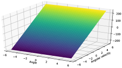
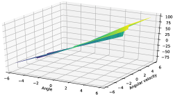
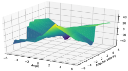
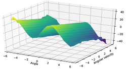
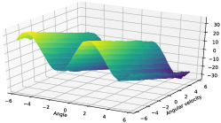
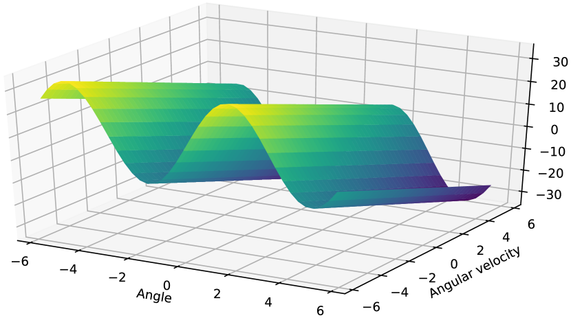
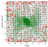
To make a visualization of the nonlinearity in the pendulum system (D.1) possible, we portray the second dynamic assuming in Fig. 1, where the first dynamic is only linear. The procedure of learning is illustrated through several stages in Fig. LABEL:Fig:learning_model. In the first column from the left, we illustrated the estimations only for the second dynamic with to be comparable to Fig. 1. Accordingly, it can be observed that the system identifier is able to closely approximate the nonlinearity with a piecewise model. More details on the uncertainty bounds obtained are provided in Appendix D.
Fig:learning_model
\subfigure
[] \subfigure[]
 \subfigure[]
\subfigure[]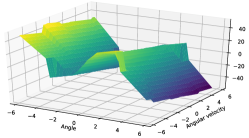 \subfigure[]
 \subfigure[]
 \subfigure
[]
6.1.2 Verification
Having the system identified and the feedback control, we can apply the verification algorithm based on MIQP problem. As done in Chen et al. (2020), we implemented the learner in CVXpy Diamond and Boyd (2016) with MOSEK ApS (2020) solver, and the verifier in Gurobi 9.1.2 Gurobi (2020).
We choose such that and . To verify the system, we ran the algorithm and obtained a matrix (who numerical values are given in Appendix D) that characterizes the Lyapunov function as in (12).
The largest level set of the associated Lyapunov function in is pictured in Fig. 2 as the the ROA of the closed-loop system. Moreover, we illustrate different trajectories of the controlled system that confirms the verified Lyapunov function by constructing an ROA around the origin.
Fig:ROA
\subfigure
[]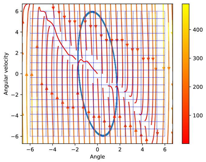 \subfigure[]
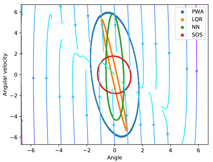
(b). The comparison results for ROA of the closed-loop system is illustrated for and , together with the trajectories of the system. The comparison results for LQR, NN, and SOS are taken from Chang et al. (2020).
6.1.3 Comparison Results
To highlight the merits of the proposed piecewise learning approach, we compare the ROA obtained by different approaches in the literature. Chang et al. (2020) proposed a neural network (NN) Lyapunov function for stability verification. According to Chang et al. (2020), the comparison done on the pendulum system with linear quadratic regulator (LQR) and sums-of-squares (SOS) showed noticeable superiority of the NN-based Lyapunov approach. Following the comparison results from Chang et al. (2020), we compare the ROA obtained by our approach with NN, SOS, and LQR techniques in Fig. 2. Clearly, the ROA obtained by the piecewise controller with the non-monotonic Lyapunov function is considerably larger than the ones obtained by NN, SOS, and LQR algorithms as shown in Chang et al. (2020).
6.2 Dynamic Vehicle System with Skidding
We have also implemented the proposed approach in a more complex dynamic vehicle system with skidding, which shows promising results. The results are omitted in the main paper due to the space limit. They can be found in Appendix D.
7 Conclusion
For regulating nonlinear systems with uncertain dynamics, a piecewise nonlinear affine framework was proposed in which each piece is responsible for learning and controlling over a partition of the domain locally. Then, in a particular case of the proposed framework, we focused on learning in the form of the well-known PWA systems, for which we presented an optimization-based verification approach that takes into account the estimated uncertainty bounds. We used the pendulum system as a benchmark example for the numerical results. Accordingly, an ROA resulting from the level set of a learned Lyapunov function is obtained. Furthermore, the comparison with other control approaches in the literature illustrates a considerable improvement in the ROA using the proposed framework. As another example, we implemented the presented approach on a dynamical vehicle system with considerably higher number of partitions and dimensions. The results demonstrated that the approach can scale efficiently, hence, can be potentially implemented on more complex real-world problems in real-time.
Acknowledgments
This work is partially supported by the HUST-WUXI Research Institute through a JITRI-Waterloo joint project, the NSERC Canada Research Chairs (CRC) program, an NSERC Discovery Grant, and an Ontario Early Researcher Award (ERA).
References
- Aeyels and Peuteman (1998) Dirk Aeyels and Joan Peuteman. A new asymptotic stability criterion for nonlinear time-variant differential equations. IEEE Transactions on automatic control, 43(7):968–971, 1998.
- Ahmadi and Parrilo (2008) Amir Ali Ahmadi and Pablo A Parrilo. Non-monotonic lyapunov functions for stability of discrete time nonlinear and switched systems. In 2008 47th IEEE conference on decision and control, pages 614–621. IEEE, 2008.
- Amaldi et al. (2016) Edoardo Amaldi, Stefano Coniglio, and Leonardo Taccari. Discrete optimization methods to fit piecewise affine models to data points. Computers & Operations Research, 75:214–230, 2016.
- Andrikopoulos et al. (2013) George Andrikopoulos, George Nikolakopoulos, Ioannis Arvanitakis, and Stamatis Manesis. Piecewise affine modeling and constrained optimal control for a pneumatic artificial muscle. IEEE Transactions on Industrial Electronics, 61(2):904–916, 2013.
- ApS (2020) MOSEK ApS. The mosek optimization toolbox for python manual, 2020.
- Atkinson and Vaidya (1995) David S Atkinson and Pravin M Vaidya. A cutting plane algorithm for convex programming that uses analytic centers. Mathematical Programming, 69(1):1–43, 1995.
- Balakrishnan et al. (2008) SN Balakrishnan, Jie Ding, and Frank L Lewis. Issues on stability of adp feedback controllers for dynamical systems. IEEE Transactions on Systems, Man, and Cybernetics, Part B (Cybernetics), 38(4):913–917, 2008.
- Baotic (2005) Mato Baotic. Optimal control of piecewise affine systems: A multi-parametric approach. PhD thesis, ETH Zurich, 2005.
- Berkenkamp et al. (2016) Felix Berkenkamp, Riccardo Moriconi, Angela P Schoellig, and Andreas Krause. Safe learning of regions of attraction for uncertain, nonlinear systems with gaussian processes. In 2016 IEEE 55th Conference on Decision and Control (CDC), pages 4661–4666. IEEE, 2016.
- Bobiti and Lazar (2016) Ruxandra Bobiti and Mircea Lazar. A sampling approach to finding lyapunov functions for nonlinear discrete-time systems. In 2016 European Control Conference (ECC), pages 561–566. IEEE, 2016.
- Borrelli et al. (2006) Francesco Borrelli, Alberto Bemporad, Michael Fodor, and Davor Hrovat. An mpc/hybrid system approach to traction control. IEEE Transactions on Control Systems Technology, 14(3):541–552, 2006.
- Boyd and Vandenberghe (2007) Stephen Boyd and Lieven Vandenberghe. Localization and cutting-plane methods. From Stanford EE 364b lecture notes, 2007.
- Boyd et al. (2004) Stephen Boyd, Stephen P Boyd, and Lieven Vandenberghe. Convex optimization. Cambridge university press, 2004.
- Breschi et al. (2016) Valentina Breschi, Dario Piga, and Alberto Bemporad. Piecewise affine regression via recursive multiple least squares and multicategory discrimination. Automatica, 73:155–162, 2016.
- Brunton et al. (2016) Steven L Brunton, Joshua L Proctor, and J Nathan Kutz. Discovering governing equations from data by sparse identification of nonlinear dynamical systems. Proceedings of the national academy of sciences, 113(15):3932–3937, 2016.
- Chang et al. (2020) Ya-Chien Chang, Nima Roohi, and Sicun Gao. Neural lyapunov control. arXiv preprint arXiv:2005.00611, 2020.
- Chen et al. (2020) Shaoru Chen, Mahyar Fazlyab, Manfred Morari, George J. Pappas, and Victor M. Preciado. Learning lyapunov functions for piecewise affine systems with neural network controllers, 2020.
- Christophersen et al. (2005) Frank J Christophersen, Mato Baotić, and Manfred Morari. Optimal control of piecewise affine systems: A dynamic programming approach. In Control and Observer Design for Nonlinear Finite and Infinite Dimensional Systems, pages 183–198. Springer, 2005.
- Dai et al. (2021) Hongkai Dai, Benoit Landry, Lujie Yang, Marco Pavone, and Russ Tedrake. Lyapunov-stable neural-network control. arXiv preprint arXiv:2109.14152, 2021.
- Diamond and Boyd (2016) Steven Diamond and Stephen Boyd. Cvxpy: A python-embedded modeling language for convex optimization. The Journal of Machine Learning Research, 17(1):2909–2913, 2016.
- Du et al. (2021) Yingwei Du, Fangzhou Liu, Jianbin Qiu, and Martin Buss. Online identification of piecewise affine systems using integral concurrent learning. IEEE Transactions on Circuits and Systems I: Regular Papers, 68(10):4324–4336, 2021.
- Elzinga and Moore (1975) Jack Elzinga and Thomas G Moore. A central cutting plane algorithm for the convex programming problem. Mathematical Programming, 8(1):134–145, 1975.
- Farsi and Liu (2020) Milad Farsi and Jun Liu. Structured online learning-based control of continuous-time nonlinear systems. IFAC-PapersOnLine, 53(2):8142–8149, 2020.
- Farsi and Liu (2021) Milad Farsi and Jun Liu. A structured online learning approach to nonlinear tracking with unknown dynamics. In 2021 American Control Conference (ACC), pages 2205–2211. IEEE, 2021.
- Farsi and Liu (2022) Milad Farsi and Jun Liu. Structured online learning for low-level control of quadrotors. In 2022 American Control Conference (ACC). IEEE, 2022.
- Ferrari-Trecate et al. (2003) Giancarlo Ferrari-Trecate, Marco Muselli, Diego Liberati, and Manfred Morari. A clustering technique for the identification of piecewise affine systems. Automatica, 39(2):205–217, 2003.
- Gambella et al. (2021) Claudio Gambella, Bissan Ghaddar, and Joe Naoum-Sawaya. Optimization problems for machine learning: A survey. European Journal of Operational Research, 290(3):807–828, 2021.
- Garulli et al. (2012) Andrea Garulli, Simone Paoletti, and Antonio Vicino. A survey on switched and piecewise affine system identification. IFAC Proceedings Volumes, 45(16):344–355, 2012.
- Geyer et al. (2008) Tobias Geyer, Georgios Papafotiou, and Manfred Morari. Hybrid model predictive control of the step-down dc–dc converter. IEEE Transactions on Control Systems Technology, 16(6):1112–1124, 2008.
- Goffin and Vial (1993) Jean-Louis Goffin and Jean-Philippe Vial. On the computation of weighted analytic centers and dual ellipsoids with the projective algorithm. Mathematical Programming, 60(1):81–92, 1993.
- Gurobi (2020) Gurobi Optimizer Gurobi. Reference manual, gurobi optimization, 2020.
- Haddad and Chellaboina (2011) Wassim M Haddad and VijaySekhar Chellaboina. Nonlinear dynamical systems and control. Princeton university press, 2011.
- Jiang and Wang (2001) Zhong-Ping Jiang and Yuan Wang. Input-to-state stability for discrete-time nonlinear systems. Automatica, 37(6):857–869, 2001.
- Kamalapurkar et al. (2018) Rushikesh Kamalapurkar, Patrick Walters, Joel Rosenfeld, and Warren Dixon. Model-based reinforcement learning for approximate optimal control. In Reinforcement Learning for Optimal Feedback Control, pages 99–148. Springer, 2018.
- Lewis and Vrabie (2009) Frank L Lewis and Draguna Vrabie. Reinforcement learning and adaptive dynamic programming for feedback control. IEEE circuits and systems magazine, 9(3):32–50, 2009.
- Liu et al. (2016) XY Liu, Stefano Alfi, and Stefano Bruni. An efficient recursive least square-based condition monitoring approach for a rail vehicle suspension system. Vehicle System Dynamics, 54(6):814–830, 2016.
- Ljung and Söderström (1983) Lennart Ljung and Torsten Söderström. Theory and practice of recursive identification. MIT press, 1983.
- Marcucci and Tedrake (2019) Tobia Marcucci and Russ Tedrake. Mixed-integer formulations for optimal control of piecewise-affine systems. In Proceedings of the 22nd ACM International Conference on Hybrid Systems: Computation and Control, pages 230–239, 2019.
- Marcucci et al. (2017) Tobia Marcucci, Robin Deits, Marco Gabiccini, Antonio Bicchi, and Russ Tedrake. Approximate hybrid model predictive control for multi-contact push recovery in complex environments. In 2017 IEEE-RAS 17th International Conference on Humanoid Robotics (Humanoids), pages 31–38. IEEE, 2017.
- Nesterov (1995) Yu Nesterov. Cutting plane algorithms from analytic centers: efficiency estimates. Mathematical Programming, 69(1):149–176, 1995.
- Pepy et al. (2006) Romain Pepy, Alain Lambert, and Hugues Mounier. Path planning using a dynamic vehicle model. In 2006 2nd International Conference on Information & Communication Technologies, volume 1, pages 781–786. IEEE, 2006.
- Rebennack and Krasko (2020) Steffen Rebennack and Vitaliy Krasko. Piecewise linear function fitting via mixed-integer linear programming. INFORMS Journal on Computing, 32(2):507–530, 2020.
- Rodrigues and Boyd (2005) Luis Rodrigues and Stephen Boyd. Piecewise-affine state feedback for piecewise-affine slab systems using convex optimization. Systems & Control Letters, 54(9):835–853, 2005.
- Rodrigues and How (2003) Luis Rodrigues and Jonathan P How. Observer-based control of piecewise-affine systems. International Journal of Control, 76(5):459–477, 2003.
- Strijbosch et al. (2020) Nard Strijbosch, Isaac Spiegel, Kira Barton, and Tom Oomen. Monotonically convergent iterative learning control for piecewise affine systems. IFAC-PapersOnLine, 53(2):1474–1479, 2020.
- Sun et al. (2002) Jie Sun, Kim-Chuan Toh, and Gongyun Zhao. An analytic center cutting plane method for semidefinite feasibility problems. Mathematics of Operations Research, 27(2):332–346, 2002.
- Sun et al. (2019) Xiaoqiang Sun, Houzhong Zhang, Yingfeng Cai, Shaohua Wang, and Long Chen. Hybrid modeling and predictive control of intelligent vehicle longitudinal velocity considering nonlinear tire dynamics. Nonlinear Dynamics, 97(2):1051–1066, 2019.
- Toriello and Vielma (2012) Alejandro Toriello and Juan Pablo Vielma. Fitting piecewise linear continuous functions. European Journal of Operational Research, 219(1):86–95, 2012.
- Vlad et al. (2012) Cristina Vlad, Pedro Rodriguez-Ayerbe, Emmanuel Godoy, and Pierre Lefranc. Explicit model predictive control of buck converter. In 2012 15th International Power Electronics and Motion Control Conference (EPE/PEMC), pages DS1e–4. IEEE, 2012.
- Wang et al. (2009) Fei-Yue Wang, Huaguang Zhang, and Derong Liu. Adaptive dynamic programming: An introduction. IEEE computational intelligence magazine, 4(2):39–47, 2009.
- Wu et al. (2015) Lifu Wu, Xiaojun Qiu, Ian S Burnett, and Yecai Guo. A recursive least square algorithm for active control of mixed noise. Journal of Sound and Vibration, 339:1–10, 2015.
- Yuan et al. (2019) Ye Yuan, Xiuchuan Tang, Wei Zhou, Wei Pan, Xiuting Li, Hai-Tao Zhang, Han Ding, and Jorge Goncalves. Data driven discovery of cyber physical systems. Nature communications, 10(1):1–9, 2019.
- Zou and Li (2007) Yuanyuan Zou and Shaoyuan Li. Robust model predictive control for piecewise affine systems. Circuits, Systems & Signal Processing, 26(3):393–406, 2007.
Appendix A Model Identification
A.1 Continuity of the Identified Model
Considering that differentiable bases are assumed, the model identified is differentiable within the interior of for . However, the pieces of the model may not meet in the boundaries of where for any and , .
Based on our knowledge of system (1) from which we collect samples the continuity holds for the original system. Hence, in theory, if many pieces are chosen, and enough samples are collected, the edges of pieces will converge together to yield a continuous model. However, choosing arbitrarily small pieces is not practical.
There exist different techniques to efficiently choose the partitions on and best fit a continuous piecewise model, see e.g. Toriello and Vielma (2012); Breschi et al. (2016); Ferrari-Trecate et al. (2003); Amaldi et al. (2016); Rebennack and Krasko (2020). Such techniques usually involve global adjustments of the model weights and the partitions for which the computations can be considerably expensive. Therefore, we choose to locally deal with the gaps among the pieces. This can be done by a post-processing routine performed on the identified model.
A rather straightforward technique is to define extra partitions in the margins of each to fill the gaps among pieces. The weights of the corresponding pieces added can be chosen according to the weights of the adjacent pieces that are given by the identification. This is done in a way that helps to connect all the pieces together to make a continuous piecewise model. Fig. 3 illustrates the process of constructing extra partitions for a two-dimensional case, where we choose them to be in triangular shapes. A similar approach can be taken for generalizing to the -dimensional case.

A.2 Database
Although an online technique is used to update the piece-wise model along trajectories, we still need to collect a number of samples for each piece of the system. The set of samples recorded will be used later to obtain an estimation of the uncertainty bounds for each mode of the system. For this purpose, we, over time, handpick and save samples that best describe the dynamics in any mode of the piecewise system.
It should be noted that the database will be processed offline to extract the uncertainty bounds. Hence, it does not affect the online learning procedure and its computational cost. Any sample of the system, to be stored in the database, includes , where the state derivative is approximated by and . For better results, higher-order approximations of the state derivative can be employed.
Different techniques can be employed to obtain a summary of the samples collected. We assume a given maximum size of the database . Then, for any mode of the piecewise model, we keep adding the samples with larger prediction errors to the database. Therefore, at any step, we compare the prediction error with the most recent average error obtained for the active piece. Hence, if the condition holds we add the sample to the database, where the constant adjusts the threshold. If the maximum number of samples in database is reached, we replace the oldest sample with the recent one.
Appendix B Analysis of Uncertainty Bounds
B.1 Proof of Theorem 4.1
Proof B.1.
According to Assumption 1, it is straightforward to show that the prediction error can be bound for any by using the samples in partition as
B.2 Quadratic Programs for Bounding Errors
Assumption 2
Assumption 3
Assumption 4
An initial estimation of and Lipschitz constants and is known.
The following results and the bounds will directly depend on the choice of , and . However, this is the least we can assume that allows us to carry out the computations. Moreover, making such assumptions is not restrictive in practice since we often have a general knowledge of the application. Moreover, the learning may be first started with an initial guess of the continuity constants. Later, if the samples collected override the assumption made, we can update these values.
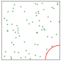
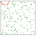
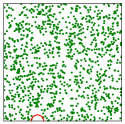
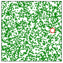
To calculate the uncertainty bound for any piece, we first look for the largest gap existing among the samples within each piece. Fig. LABEL:fig:subfigex illustrates an example of how this gap is affected by the number of samples in a particular mode. To obtain the radius, we solve a quadratic programming (QP) problem for each piece. The solution to the following QP returns the centre at which an -dimensional ball of the largest radius can be found in the th piece such that no samples are contained in this ball:
| (20) | ||||
Similarly, we can obtain the centre and radius to represent the sample gap as an -dimensional ball in the control space by solving
| (21) | ||||
fig:subfigex
\subfigure[]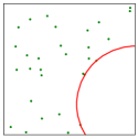 \subfigure[]
 \subfigure[]
 \subfigure[]
 \subfigure[]
B.3 Proof of Theorem 4.2
Proof B.2.
According to the Lipschitz condition, the following holds for any
| (22) |
Moreover, we have the estimation of the system. Then, the difference is bounded by
where we used inequality (B.2) and the bound obtained in Theorem 4.1 according to the samples. Moreover, considering that the identified model is known, we can easily compute the corresponding Lipschitz constants and . The largest distance with the closest sample happens in the sample gap given with the radius , and . This yields the total bound of the error as
Appendix C Verification
C.1 Searching for a Lyapunov Function
We summarize an altered version of the technique for obtaining a Lyapunov function that is first presented in Chen et al. (2020) for a deterministic closed-loop system with the neural network controller. Hence, we modify the algorithm to allow the uncertainty together with the feedback control (7).
The procedure includes two stages that are performed iteratively until a Lyapunov function is obtained and verified, or it is concluded that there exists no Lyapunov function in the given set of candidates.
In the first stage, we assume an initial set of Lyapunov candidates in the form of (12). Then, the learner searches for a subset for which the negativity of the Lyapunov difference can be guaranteed with respect to a set of samples collected from the system. If such a subset exists, one element in this subset is proposed as the Lyapunov candidate by the learner.
In the second stage, the proposed Lyapunov candidate is verified on the original system. Noting that the learner only uses a finite number of samples for suggesting a Lyapunov candidate, it may not be valid for all the evolutions of the uncertain system. Accordingly, the verifier either certifies the Lyapunov candidate, or finds a point as the counter-example for which the Lyapunov candidate fails. This sample is added to the set of samples collected from the system. Then, we again proceed to the learner stage with the updated set of samples.
The algorithm is run in a loop, where we start with an empty set of samples in the learner. Then, we continue with proposing a Lyapunov candidate, and adding one counter-example in each iteration of the loop. While growing the set of samples, the set of Lyapunov candidates shrinks in every iteration until one is either validated, or no element is left in the set meaning that no such Lyapunov exists.
C.2 Convergence of ACCPM
The convergence and complexity of the ACCPM for searching a quadratic Lyapunov function is discussed in Sun et al. (2002); Chen et al. (2020), where an upper bound is obtained for the number of steps taken until the algorithm exits.
Lemma C.1.
Let be a convex subset of . Moreover, there exists such that , where Frobenius norm is used, and . Then, the center cutting-plane algorithm concludes in at most steps.
C.3 Stability Analysis (Proof of Theorem 5.1)
Proof C.3.
According to the conditions of the verifier, if the optimal value returned by the MIQP (14) is negative, we have effectively verified the following Lyapunov conditions:
| (23) | |||
| (24) |
for the uncertain closed-loop system (11). By standard Lyapunov analysis for set stability Haddad and Chellaboina (2011); Jiang and Wang (2001), the set , which is the ball of radius in infinity norm around the origin, is asymptotically stable for system (11). Furthermore, any sub-level set of , i.e., for some , contained in is contained in the ROA of .
Remark C.4.
Due to the existence of a non-zero additive uncertainty bound, one cannot expect convergence to the origin precisely. This issue is addressed by providing convergence guarantee to a small neighborhood of the origin, i.e., . By collecting enough samples around the origin, a local approximation of the system is obtained by the mode of the identified system, whose domain includes the origin, while can be made arbitrarily small as . By doing so, we can make in Theorem 5.1 arbitrarily small and the stability result is practically equivalent to the asymptotic stability of the origin. Alternatively, one can assume that there exists a local stabilizing controller that one can switch to when entering a small neighborhood of the origin. In this case, asymptotic stability can be achieved.
Appendix D Numerical Results
It should be noted, the learning is started from the mode containing the origin in its domain, that we label by . As we collect more random samples in , we can effectively decrease the uncertainty of the model around the origin, and obtain a local controller. Then, we gradually expand the areas sampled to train the rest of the pieces in the PWA model.
Fig. LABEL:Fig:uncertainty depicts the uncertainty bound obtained over the ROI, where a decreasing magnitude through different stages of learning, i.e. subfigures () to (), is evident. Fig. LABEL:fig:samples illustrates a map of the pieces on together with the samples and the sample gaps for each piece as discussed in Appendix B.2.
Remark D.1.
It is worth mentioning that the model obtained and the uncertainty bounds can be further improved by continuing the sampling. In this implementation, we perform sampling only until the uncertainty bound obtained allows us to verify a decreasing value function for each piece of the PWA system.
Fig:uncertainty
\subfigure[] \subfigure[]
 \subfigure[]
\subfigure[] \subfigure[]
 \subfigure[]
fig:samples
\subfigure[]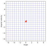 \subfigure[]
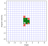 \subfigure[]
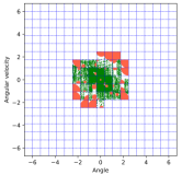
\subfigure[]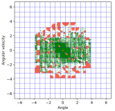 \subfigure[]
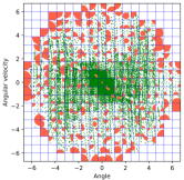 \subfigure[]
D.1 Pendulum System
The state space description of the system is given as
| (25) |
where the parameters are taken from Chang et al. (2020) ( = 9.81, = 0.5, = 0.15, = 0.1). The performance criteria are defined by the choices of , .
D.2 The Learned Matrix \texorpdfstringLg
D.3 Dynamic Vehicle System
According to Pepy et al. (2006), we present the dynamic model of the vehicle implemented. Let us define the states and as the coordinate of the center of gravity in the 2D space, as the orientation of the vehicle, as the lateral velocity, and as the rate of the orientation. Moreover, the input of the system is given by the front-wheel angle . Then, by assuming a constant longitudinal velocity , the dynamical model of the vehicle can be written as
where , and denote the cornering stiffness coefficients of the front and rear wheels. Moreover, the distance of the center of gravity from the front and rear wheels are given by , and .
D.4 Numerical Results for the Dynamic Vehicle System
In this section, to better demonstrate the merits of the algorithm proposed, we implemented the approach on a more complex system. The kinematic model of the vehicle system does not consider the real behavior of the system at high speeds where skidding is possible. Therefore, Pepy et al. (2006) proposed a more realistic dynamical model of the vehicle which is implemented in this paper.
D.4.1 Identify and Control
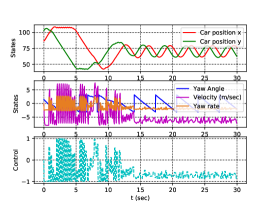
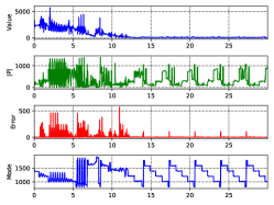
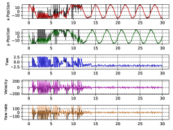
Control objective is to minimize the distance of the vehicle from the goal point in the 2D map. To achieve the objective, we run the vehicle from some random initial position and yaw values. Then, the identification and control procedures are done in a loop through different episodes. The longitudinal velocity of the vehicle is assumed to be constant in this system similar to Pepy et al. (2006). Therefore, to minimize the cost given by the control objective, the vehicle converges to some circular path around the goal point, which is indeed the optimal path for the problem defined. Fig. LABEL:Fig:results_vehicle, contains the simulation results within an episode of learning, including the state and control signals, prediction error for each state, the value function and the modes.
D.5 Comparison of Runtime Results
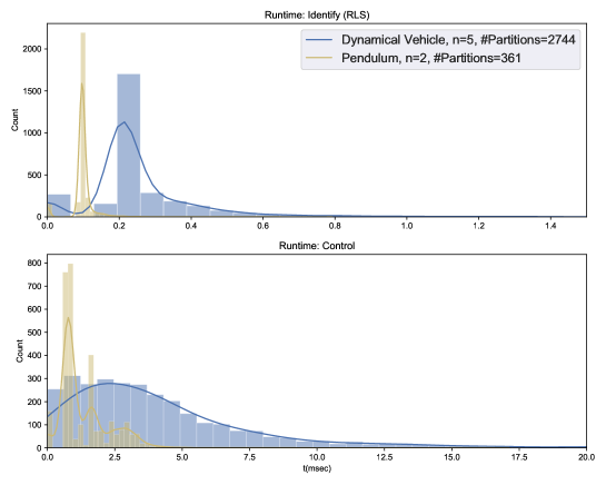
To analyze the computational aspects of the proposed technique, we provide the runtime results while learning the dynamics and obtaining the control for both examples implemented. The proposed framework is considered as an online technique. Hence, in the applications, the computational complexity of the real-time identification and control becomes more important. Therefore, we here focus in the complexity of the online learning procedure rather than the verification technique which can be done offline. Fig. 9 includes the runtime results separately for the identification and control units. Accordingly, the identifier and the controller can be updated in at most and respectively. Accordingly, it can be observed that for the higher dimensional system with an also larger number of partitions, the computations still remain in a tractable size that can allow real-time applications, considering the nature of the systems.
Fig:results_vehicle
\subfigure
[] \subfigure[]
 \subfigure[]
(). The graph denotes the evolutions of the value function, the norm of the control parameters for the active mode, the prediction error, and the active mode of the piecewise model that correspond to the results in Fig 8. It can be seen that the value function learned is minimized.
(). Corresponding to Fig. 8 and 8, the prediction results of the learned model is compared with the original system within an episode of learning. It can be observed that the prediction signals shown by the black lines can match the ones obtained from the original dynamics.
