Too Big to Fail? Active Few-shot Learning Guided Logic Synthesis

Abstract

Generating sub-optimal synthesis transformation sequences (“synthesis recipe”) is an important problem in logic synthesis. Manually crafted synthesis recipes have poor quality. State-of-the art machine learning (ML) works to generate synthesis recipes do not scale to large netlists as the models need to be trained from scratch, for which training data is collected using time consuming synthesis runs. We propose a new approach, Bulls-Eye, that fine-tunes a pre-trained model on past synthesis data to accurately predict the quality of a synthesis recipe for an unseen netlist. This approach on achieves 2x-10x run-time improvement and better quality-of-result (QoR) than state-of-the-art machine learning approaches.

I Introduction

There is a growing academic and industry interest in using machine learning (ML) techniques in design automation problems [1, 2, 3]. Several problems in electronic design automation (EDA), such as logic synthesis, placement and routing, and VLSI testing are combinatorial optimization problems that require sequential decision-making to achieve the target objective. Logic synthesis, the first step in an EDA flow, applies a sequence of synthesis transformations (i.e., a “synthesis recipe”) to an and-inverter-graph (AIG) representation of a Boolean function to minimize its size or depth. For instance, the transformation heuristics in ABC [4], a leading academic synthesis tool, include steps like balance, refactor, rewrite, etc. In this work, we focus on ML-guided search for “good” logic synthesis recipes; a problem that has received much recent attention.

Traditionally, EDA engineers choose from a set handcrafted synthesis recipes, for instance, resyn2 or compress2rs [4] based on intuition and experience. Yet, the space of all synthesis recipes is vast; recent work has shown ML-guided exploration of this vast solution space can yield synthesis recipes that are tailored for each design and outperform handcrafted recipes in terms of quality-of-result (QoR) [5, 6, 7, 8]. In these papers, finding a good synthesis recipe is formulated as a classification problem [5]—which seeks to distinguish good “angel” recipes from bad “devil” recipes—or as in [6, 7, 8] as an Markov decision process (MDP) that is solved using reinforcement learning (RL). However, the prior work is deficient on two fronts: (1) scalability to large designs; and (2) generalizability to previously unseen netlists. Typically, models are trained from scratch, requiring significant training time and a large number of synthesis runs for large unseen designs; and leaving prior experience untapped. For this reason, in [12], “benchmarks were excluded from the experimentation which showed significant training times, being large circuits”.

The underlying issue is that ML methods rely on high-quality labeled data (or reward signals for RL)—in logic synthesis, the input features are AIGs and synthesis recipes, and the resulting QoRs are labels/rewards. For each new design, prior work obtains labels/rewards (i.e., QoRs) by synthesizing the design using a large number of synthesis recipes; however, this is prohibitively time-consuming for large designs. An alternative is to use fewer synthesis runs, or even a model trained on previously seen designs, but this results in lower quality synthesis recipes.

In this paper, we propose a new logic ML-guided synthesis solution that addresses these limitations and scales to large designs on which existing state-of-the-art (SOTA) solutions fail or time-out. Bulls-Eye has two key ideas: (1) few-shot learning: fine-tuning a base model trained on previously seen designs using only a few training samples from the new design; and (2) active learning: fine-tuning can be further improved by intelligently picking the synthesis recipes for which we obtain QoRs/labels given a limited synthesis run budget. We illustrate these ideas using Bulls-Eye, a framework that uses a graph convolutional network (GCN) as a QoR predictor, and simulated annealing (SA) to search the design space. The core ideas proposed are general and apply to other ML-guided synthesis frameworks also. To summarize, our key contributions are:

• Bulls-Eye: an active few-shot learning approach that transfers knowledge from a base model trained on past data to train a new model that predicts the QoR of a synthesis run for an unseen netlist; and uses simulated annealing to find an optimized synthesis recipe for the new netlist.

• Scalability to large benchmarks: Bulls-Eye’s base model can be learned on small designs for which training data is easy to generate; and transferred using only a few, smartly selected synthesis runs (i.e., ”shots”) to large, unseen netlists. Bulls-Eye produces high-quality synthesis recipes for benchmarks on which SOTA methods fail or time-out.

• Bulls-Eye achieves better QoR with 2x-10x run-time speed-up and more than 7x speed-up on large benchmarks compared to conventional approaches. Compared to prior SOTA, Bulls-Eye achieves better QoR with an average 1.04x ( vs. [8]) and 11.21x (vs. [7]) run-time speedup.

II Preliminaries and Related work

II-A Logic Synthesis

Logic synthesis transforms a hardware design in a high-level abstraction (e.g., register-transfer level) to a gate-level netlist, ultimately mapping to a user-specified technology library. Typically, logic synthesis tries to minimize the circuit area and meet a specific delay constraint. Logic synthesis is performed in a series of steps: (1) the design is converted to a generic netlist-level representation (e.g., AIG), (2) the netlist undergoes heuristics-based optimization to implement the same functionality using fewer gates and/or reduced depth which correlates to a reduction in the final area and delay of design [2], (3) technology mapping of the generic netlist using standard cells, and (4) post-mapping optimizations. Consistent with prior works, we focus on the pre-technology mapping optimization of generic gate-level netlists.

TABLE I: Work on ML-based synthesis recipe generation

Prior work	Input Features	ML techniques	Max. nodes considered	Model transferability
[9]	MIG	GCN, RL	$\leq$2000	✗
[5]	Flow encoding	CNN	44045	✗
[6]	AIG encoding	RL	176938	$\dagger$
[10]	-	MAB	30003	✗
[7]	AIG+state encoding	GCN, RL	2675	✗
[8]	AIG+state encoding	GCN,RL	32060	✗
Bulls-Eye	AIG+recipe encoding	GCN,CNN	114771	✓

$\dagger$ DRiLLS claims the model can be reused, without empirical evaluation

ABC [4] is the current state-of-the-art framework for optimizing AIG-based netlists. AIGs are directed acyclic graphs and ABC’s synthesis transformation heuristics perform local sub-graph-level optimization to reduce the AIG structure. ABC’s well-known transformations are refactor, rewrite, re-substitute (these reduce the nodes), and balance (for depth-reduction). For $\mathbf{M}$ unique synthesis transformations, $\{\mathbf{T_{1}},\mathbf{T_{2}}...\mathbf{T_{M}}\}$ in a synthesis recipe $\mathbf{S}$, the possible number of synthesis recipes of length $\mathbf{L}$ is $\mathbf{M}^{\mathbf{L}}$ (with repeatable transformation). This indicates that the search space of possible synthesis recipes is huge. The problem of optimal synthesis recipe generation for a given AIG is:

$$\operatorname*{argmin}_{\mathbf{S}}QoR(\mathcal{G}(\mathbf{AIG},\mathbf{S}))$$ (1)

where $\mathcal{G}$ is the synthesis function defined as $\mathcal{G}:AIG\times S\longrightarrow AIG$ and $QoR$ is a function that evaluates the quality of the synthesis (i.e., lower number of nodes/depth of AIG is better).

II-B Prior work

We summarize prior work on ML for logic synthesis in Table I. Recent enhancements in logic synthesis have built on recent successes of supervised learning and RL approaches for solving sequential decision making problems [11, 1] in an attempt to find good synthesis recipes in the vast space of possible recipes. In [9, 6, 7, 8], authors generate optimal synthesis by formulating the problem as an MDP and training a policy gradient agent over a collection of synthesis runs on a set of benchmarks. During inference, the trained agent (in exploit phase) predict the best synthesis recipe for a given AIG. Authors in [9, 6] use handcrafted features from AIGs (i.e. number of AND and NOT gates, depth, number of primary inputs and outputs) to represent AIG state. Zhu et al. use handcrafted features with GCN embedding of AIG to represent current AIG state [7]. These works show results that improve upon handcrafted recipes like resyn2. In an alternate approach, Yu et al. classify an unseen synthesis recipe as good (“angel”) or bad (“devil”) by training a model on the results corresponding to a set of recipes for a design [5]. However, the trained model is design specific; a model trained on one design cannot be reused for another.

III Pitfalls of existing approaches

Black-box optimization techniques (e.g., simulated annealing or RL methods in prior work) need feedback in terms of the cost (or reward) of actions; in the logic synthesis context, the action is a synthesis recipe $\mathbf{S}$ and the cost/reward is $\mathcal{G}(\mathbf{AIG},\mathbf{S})$, obtained by synthesizing $\mathbf{AIG}$ using $\mathbf{S}$. Typically a large number of cost/reward evaluations, or equivalently, synthesis runs, are required to obtain good solutions. The biggest challenge here is that even a single synthesis run for modern complex system-on-chip (SoC) designs can require several hours or days, which limits the number of synthesis runs that can be performed in a limited time budget, and consequently, the amount of training data that can be collected and the fraction of design space that can explored. A black-box optimizer can cover in a limited time. Hence, although RL-based approaches have shown promise in generating good quality synthesis recipes, they cannot scale up to industrial-sized benchmarks [7, 8]. These observations indicate the following key questions computationally-efficient ML-enhanced logic synthesis:

• How can we predict the best synthesis recipe for a new, unseen netlist using only a limited or budgeted number of synthesis runs of that netlist?

• Given a budget, which synthesis recipes should be selected to train an accurate model for the new netlist?

• How can we efficiently leverage past information, specifically, synthesis runs on previously seen netlists to improve solution quality?

We next present Bulls-Eye, that solves the key roadblocks towards computationally efficient ML-guided logic synthesis.

IV The Bullseye framework

To reduce the cost of running actual synthesis during black-box optimization, Bulls-Eye trains a QoR predictor, $\mathbf{\hat{F}}(\mathbf{AIG},\mathbf{S},\mathbf{\theta})$, which predicts the QoR for a given $\mathbf{AIG}$ synthesized using an $L$-length synthesis recipe $\mathbf{S}$. We now seek to solve the following problem:

$$\operatorname*{argmin}_{\mathbf{S}}\mathbf{\hat{F}}(\mathbf{AIG},\mathbf{S},\mathbf{\theta})$$ (2)

$$\mathbf{\hat{F}}\approx QoR(\mathcal{G}(\mathbf{AIG},\mathbf{S}))$$

where $\mathbf{\theta}$ represents the QoR predictor’s model parameters, and $\epsilon$ represents model noise that we also seek to minimize.

IV-A Insights from ML domain

Unlike ML application in computer vision, the diversity of circuit characterization in terms of size, complexity, functionalities is not well studied and understood. We borrow two important insights from core ML community to solve our problem of learning proxy model with limited data.

Insight 1: In computer vision, various deep learning networks learn robust embeddings and are pre-trained on large dataset like Imagenet [12]. The pre-trained models are fine-tuned later for specific applications.

This helps us adopt a similar strategy and study its applicability in EDA. Large circuit designs have smaller known IP designs as building blocks; therefore pre-training a model using labelled data on small sized IP designs followed by finetuning can help predict important parameters of downstream tasks. Thus, a one-time training with labelled data on small IP designs (varied functionality) can be a qualitative QoR predictor.

Insight 2: Few-shot learning [13] learns a hypothesis function with limited labeled data of target task; however abundant labeled data is available for different tasks. Effectively, it uses transfer learning approach for classification/regression task using limited labeled data of target task.

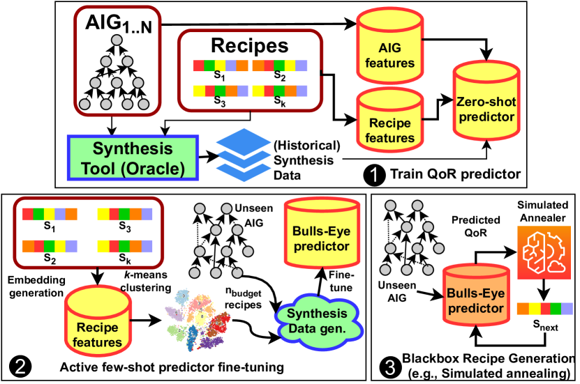
This insight guide us in our problem context for solving the problem of data scarcity, knowledge transfer and picking best-possible synthesis scripts (few-shots) to generate the labelled data. We solve this problem in three steps, illustrated in Figure 2. ➊ First we train a zero-shot QoR predictor using prior synthesis data; as we show, it is sufficient to use small benchmarks to train this zero-shot model. ➋ Next we fine-tune the zero-shot model using a small number of smartly selected synthesis runs of the AIG being optimized; and ➌ we deploy the fine-tuned QoR predictor within a black-box SA optimizer.

IV-B Zero-Shot QoR predictor (➊)

We assume that a design house has access to data from previously synthesized designs or can quickly generate data by running synthesis on small designs. We also developed OpenABC-D [14]), an open-source automated synthesis data generation framework used to generate data and train our Zero-shot predictor.

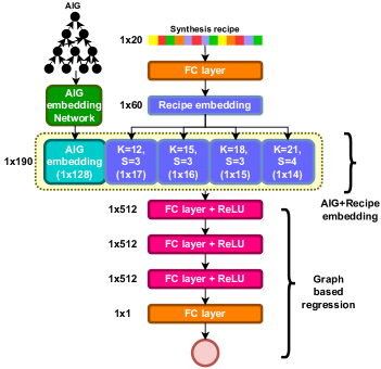
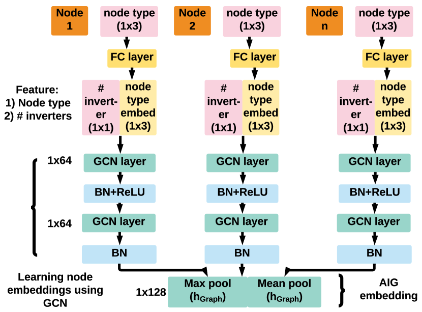
In this work, we adopt a GCN-based architecture for the predictor (Figure 1); GCNs have been used in RL-based approaches as well [8, 7], but with different architectures. Our predictor architecture is shown in  Figure 1a and contains two parallel paths. The first path takes an AIG as input and create an AIG embedding of the network; the second path extract features from synthesis recipe and outputs a “synthesis recipe embedding”. We now describe the “AIG embedding” network and recipe embedding network:

((a))

((b))

Figure 1: Architecture for QoR prediction. $GCN$: Graph convolutional layer. $FC$: fully connected layers. $BN$: Batch normalization layer.

IV-B1 AIG embedding

We leverage GCN to represent the original AIG graph. GCN can learn and extract key features from DAG structures; particularly subgraph structures that can be optimized via various synthesis transformations. GCNs make our model generalize over different AIGs structures. For AIG embedding, we consider two features for each node: type and # inverter in fan-in. The type of node can be primary input (PI), primary output (PO) or internal node. As shown in Figure 1a, we encode $nodetype$ and pass it via a linear layer. The initial node level features pass through two consecutive GCN layers aggregating local neighbourhood information based on connectivity. We use batch-norm followed by ReLU operation after each GCN layer. The graph level embedding is a readout like global pool operation on all node embeddings. We choose concatenation of average pooling and max pooling to produce the AIG embedding $h_{AIG}$. Formally, the embeddings are defined as follows:

$$h^{k}_{u} =\sigma(W_{k}\times\sum_{u\cup N(u)}\frac{h^{k-1}_{u}}{\sqrt{N(u)}\times\sqrt{N(v)}}+b_{k}),k\in[1,2]$$ (3)

$$h_{AIG} =\frac{1}{|V|}\sum_{u\in V}h^{k}_{u}\parallel\max_{u}h^{k}_{u}$$ (4)

where $h^{k}_{u}$ is GCN embedding generated by $k$th layer of node $u$. $W_{k}$ and $b_{k}$ are GCN parameters and $\sigma$ is non-linear ReLU activation. $N(\cdot)$ denotes 1-hop neighbors.

IV-B2 Synthesis recipe embedding

In our work, we consider a fixed length synthesis recipe $\mathbf{L}$. We numerically encode the recipe using available synthesis transformation and pass it through a linear layer. Next, a set of one-dimensional convolutional neural networks with different kernel length extract features to produce “synthesis recipe embedding” ($h_{recipe}$). Mathematically, it can be shown as follows:

$$h_{recipe} =concat_{i}(b_{i}+\sum_{l=j}^{j+M}s_{kl}W^{l}_{i}),i\in[1,4]$$ (5)

where $M$ is kernel length and ($W_{i}$,$b_{i}$) are filter parameters.

The Bulls-Eye zero-shot predictor is created by concatenating AIG and synthesis recipe embeddings followed by four fully connected layers that output a QoR prediction ( Figure 2). Assuming a training dataset, $\mathcal{D}_{train}$, comprising AIGs ($g_{i}$), synthesis recipes ($s_{i}$), and labels represented by number of nodes ($y_{i}$)—normalized to respective samples of design in the dataset—the graph-based regression learns a parameterized function $\hat{F}(\cdot;\theta_{ZS})$ by minimizing the loss function

$$\mathcal{L}(y,\hat{y})=\frac{1}{|\mathcal{D}_{train}|}\sum_{(g_{i},s_{i})\in\mathcal{D}_{train}}\lVert y_{i}-\hat{F}(g_{i},s_{i};\theta_{ZS})\rVert_{2}^{2}.$$ (6)

Figure 2: The Bulls-Eye framework

IV-C Fine-tuning QoR predictor (➋)

One can use the zero-shot model to predict QoR of different synthesis recipes on a new AIG. However, the accuracy of the model might be low if the features of the new AIG are different from prior data. To address this problem, we propose to fine-tune the zero-shot model using a limited number, $n_{budget}$, of synthesis runs on the new AIG, where $n_{budget}$ is specified by the designer depending on the amount of time they are willing to spend.

Fine-tuning the zero-shot predictor avoids the need to train a model from for each new design, which was a critical roadblock for prior work. This strategy has been successful in a variety of other domains, for example, image classification [15], but has not been explored for ML-guided synthesis. The next question we seek to answer is: How should the synthesis budget $n_{budget}$ be used?

We explore two solutions. The first solution, that we refer to as FT+R fine-tunes the zero-shot model using randomly selected synthesis recipes. However, the aim of the designer is to pick best synthesis recipes giving wide variations in the synthesis output. This problem can be mapped similarly to an active learning problem where label generation is a costly operation and therefore needs careful picking of data-points. Inspired by active learning approach [16], we propose a smarter solution, FT+A. Here, we cluster the embeddings of the synthesis recipes used to train the zero-shot model (recall that each recipe has its own embedding denoted by $h_{recipe}$) into $n_{budget}$ clusters, and pick the cluster heads as our candidates. The intuition behind this idea is that the cluster heads represent maximally diverse and informative points in the solution space. We synthesize the unseen AIG using the recipe cluster heads, generate labels and fine-tune $\hat{F}(\cdot;\theta_{ZS})$ to produce a high-quality QoR predictor.

Data: Unseen AIG ($g_{U}$); Zero-shot predictor: $\hat{F}(\cdot;\theta_{ZS})$; synthesis recipes ($S$): $\{s_{i},i\in[1,1500]\}$, Synthesis budget runs: $n_{budget}$

Result: Active learning aided QoR predictor: $\hat{F}(\cdot;\theta^{A}_{FT})$

Create recipe embedding $h_{S}\leftarrow\{h_{s_{i}}\forall s_{i}\in S\}$ using $\hat{F}(\cdot,\theta_{ZS})$.

$S_{cluster}\leftarrow k$-means clustering using $n_{budget}$ heads on $h_{S}$.

Synthesize and generate labeled data $D_{U}\leftarrow\{(g_{U},s_{k},y_{k})|s_{k}\in S_{cluster},|S_{cluster}|=n_{budget}\}$.

Fine-tune learnable parameters $\theta_{FT}^{A}\leftarrow\theta_{ZS}-\alpha\nabla_{\theta}\mathcal{L}(\theta,\mathcal{D}_{U})$

Algorithm 1 Active learning based model fine-tuning

Data: Initial temperature ($T_{initial}$); Max. oracle queries : $Q_{max}$; Fine-tuned QoR predictor $\hat{F}(\cdot;\theta_{FT}^{A})$, Design: ($AIG_{U}$)

Result: Node optimized synthesis recipe: $s^{*}\in M^{L}$

$T\leftarrow T_{initial}$, $Q\leftarrow 0$, $s^{*}\leftarrow$ RandomRecipe()

while $Q<Q_{max}$ do

       $s_{next}\leftarrow$ NEIGHBOUR($T,s^{*}$) $\triangleright$ Neighbour recipes

       $\Delta E\leftarrow$ ENERGY($s_{next},\hat{F}(\cdot;\theta_{FT}^{A})$) $-$ ENERGY($s^{*},\hat{F}(\cdot;\theta_{FT}^{A})$) $\triangleright$ Energy $\downarrow\Rightarrow$ no. of nodes $\downarrow$

       if $\Delta E<0$ or random() $<$ ACCEPT($T,\Delta E$) then

            $s^{*}\leftarrow s_{next}$

      $T\leftarrow$ COOLING($T,s^{*}$); $Q\leftarrow Q+1$ $\triangleright$ Annealing schedule

return $s^{*}$ $\triangleright$ Best synthesis recipe

Algorithm 2 Simulated Annealing based recipe generator

IV-D Black-box Optimization (➌)

Although Bulls-Eye (the zero-shot and fine-tuned predictors) can be used in a wide variety of black-box approaches (e.g., evolutionary algorithms), we focus on SA adopted in [17]. A good QoR predictor provides fast and accurate feedback to the optimizer by estimating the QoR of a synthesis recipe for an AIG. As we will show in our experimental evaluation, QoR predictor aided SA can substantially explore the synthesis recipe space in a given time span. Algorithm 2 outlines the flow for generating synthesis recipes. The terminology in Algorithm 2 is based on the SA literature; readers can peruse [17] for more background.

V Data generation and analysis

	Characteristics
Benchmark	PI	PO	Nodes	Depth
spi [18]	254	238	4219	35
i2c[18]	177	128	1169	15
ss_pcm[18]	104	90	462	10
usb_phy[18]	132	90	487	10
sasc[18]	135	125	613	9
wb_dma[18]	828	702	4587	29
simple_spi[18]	164	132	930	12
pci[18]	3429	3157	19547	29
ac97_ctrl[18]	2339	2137	11464	11
mem_ctrl[18]	1187	962	16307	36
des3_area[18]	303	64	4971	30
aes[18]	683	529	28925	27
sha256[19]	1943	1042	15816	76
fir[19]	410	351	4558	47
iir[19]	494	441	6978	73
tv80[18]	636	361	11328	54
fpu[20]	632	409	29623	819
dynamic_node[21]	2708	2575	18094	33
apex1[22]	45	45	1577	14
bc0[22]	26	11	1592	31
c1355[23]	41	32	512	29
c5315[23]	178	123	1613	38
c6288[23]	32	32	2337	120
c7552[23]	207	107	2198	30
dalu[22]	75	16	1735	35
i10[4]	257	224	273	58
k2[22]	45	45	2289	22
mainpla[22]	27	54	5346	38
div[24]	128	128	57247	4372
log2[24]	32	32	32060	444
max[24]	512	130	2865	287
multiplier[24]	128	128	27062	274
sin[24]	24	25	5416	225
sqrt[24]	128	64	24618	5058
square[24]	64	128	18484	250
aes_xcrypt[25]	1975	1805	45840	43
aes_secworks[26]	3087	2604	40778	42
bp_be[27]	11592	8413	82514	86
wb_conmax[18]	2122	2075	47840	24
ethernet[18]	10731	10422	67164	34
jpeg[18]	4962	4789	114771	40
tiny_rocket[21]	4561	4181	52315	80
picosoc[20]	11302	10797	82945	43
vga_lcd[18]	17322	17063	105334	23

TABLE II: Open source design characteristics (unoptimized). Primary Inputs (PI), Primary outputs (PO)

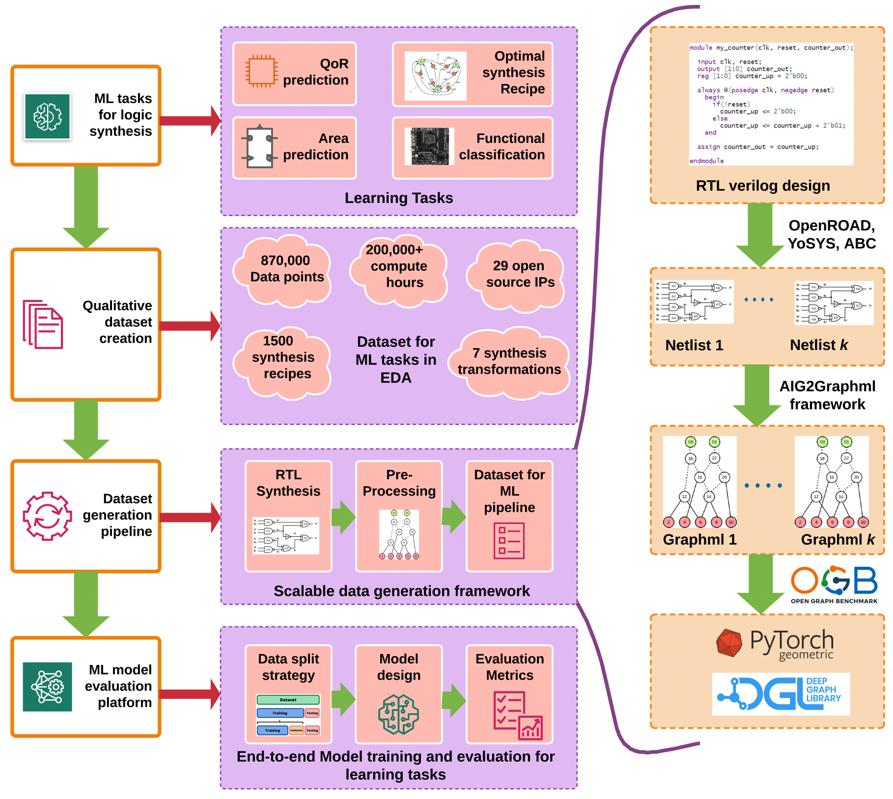
For wider access and reproducible, we focus on open source EDA platforms as key to advancing ML research in EDA. Thus, we develop OpenABC-D framework(Figure 3): an end-to-end large-scale data generation framework for augmenting ML research in circuit synthesis and making it freely available. We applied the OpenABC-D framework on a set of open source designs to generate dataset for training our Bulls-Eye predictor.

Figure 3: OpenABC-D framework

((a)) Top $1\%$

((b)) Top $5\%$

((c)) Top $10\%$

Figure 4: Correlation plots amongst top $k\%$ synthesis recipes various IPs. Darker colors indicate higher similarity between the top synthesis recipes for the pair of IPs.

V-A Data generation

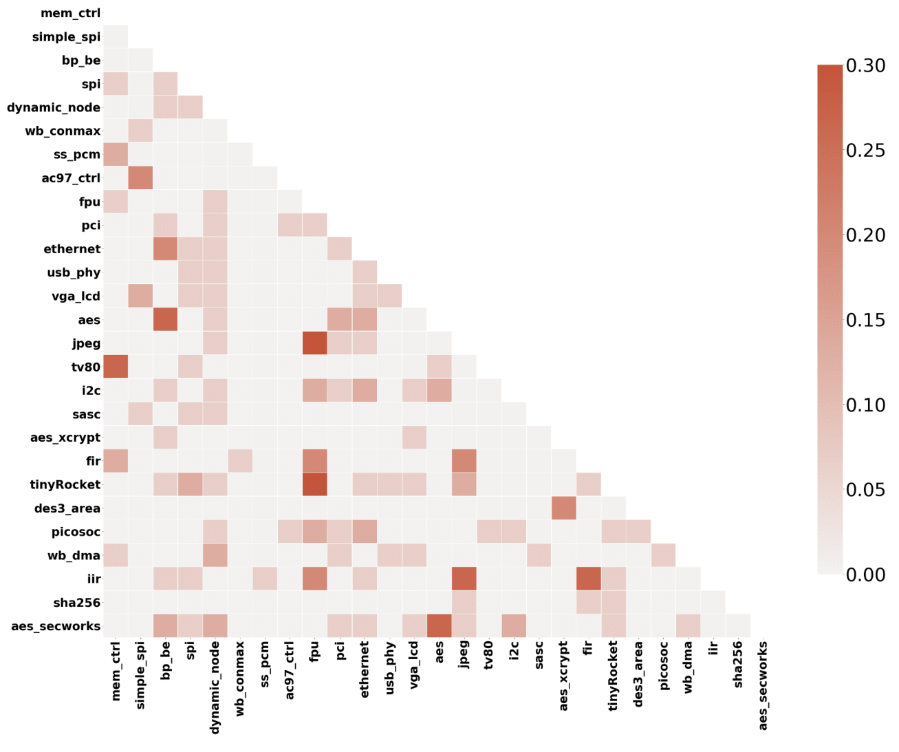
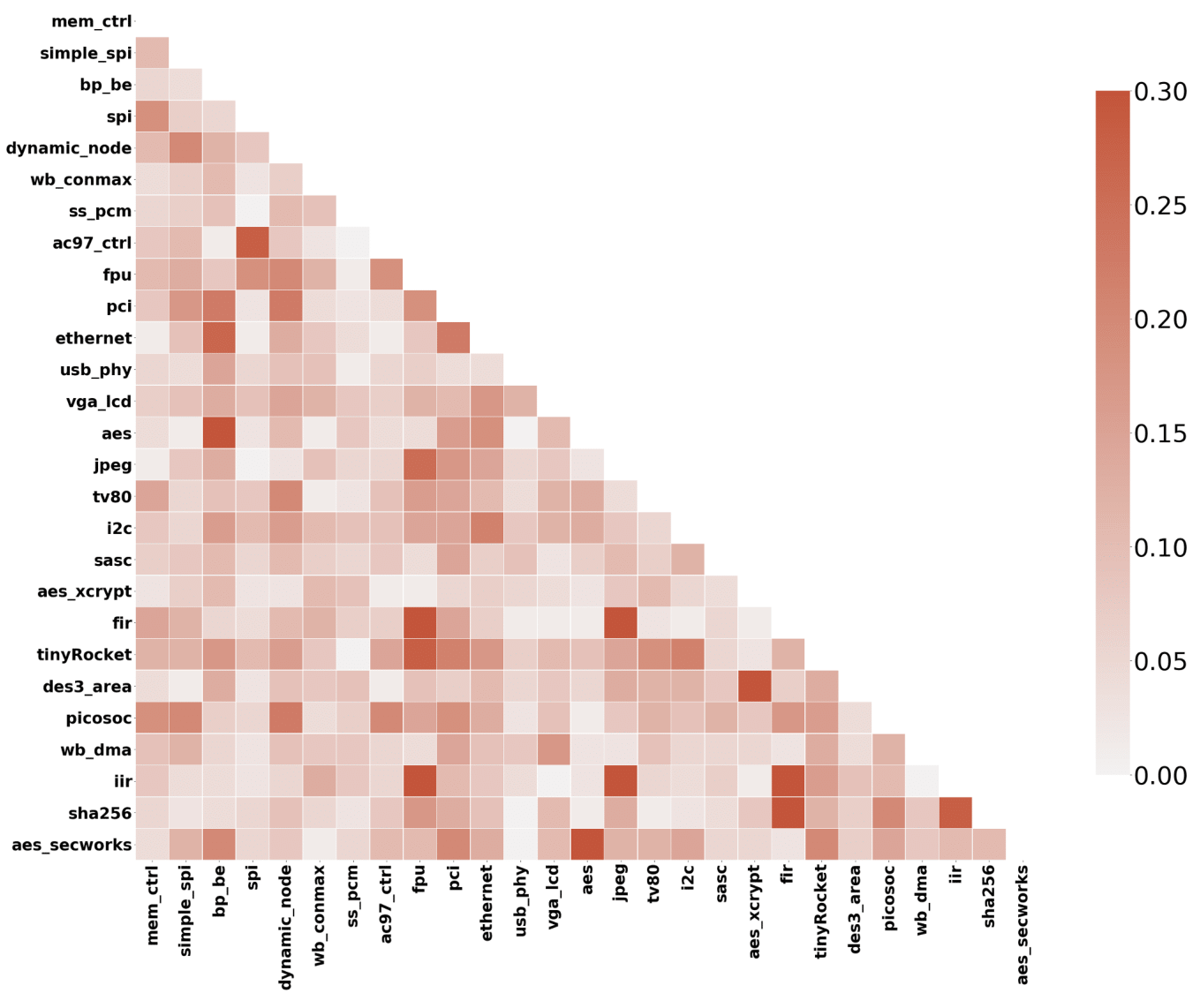
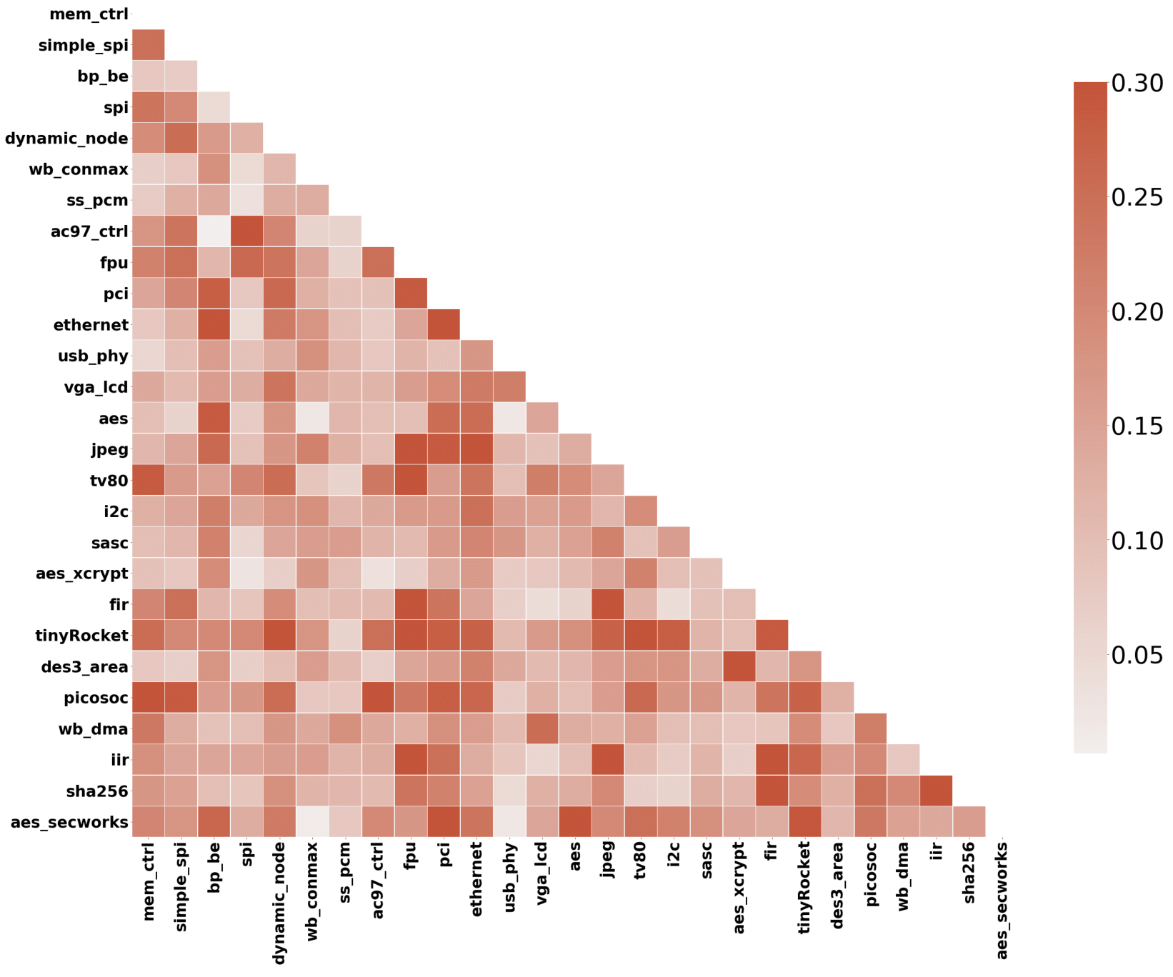
To produce the OpenABC-dataset, we use 44 open source designs with a wide range of functions. In the absence of a preexisting dataset like ImageNet [15] that represents many classes of designs, we hand-curated designs of different functionalities from MIT LL labs CEP [19], OpenCores [18], IWLS [28], ISCAS [23, 29], MCNC [22] and EPFL benchmarks [24]. These benchmarks include more complex and functionally diverse compared to only ISCAS [23, 29] and EPFL [24] benchmarks that are used in prior work and represent large, industrial-sized designs. In the context of EDA, functionally diverse IPs should have diverse AIG structures (e.g., tree-like, balanced, and skewed) that mimic the distribution of real hardware designs. Table II summarizes the structural characteristics of the data before synthesis (without optimizations). These designs are functionally diverse – bus communication protocols, computing processors, digital signal processing cores, cryptographic accelerators and system controllers. We prepared $K=1500$ synthesis recipes each $L=20$ long, comprising a mix of rewrite, re-substitute, refactor, rewrite -z, resub -z, refactor -z and balance transformations, consistent with prior works [7, 8, 6]. The synthesis recipes were prepared by randomly sampling from the set of synthesis transformations, assuming a uniform distribution. We ran synthesis with abc using server-grade Intel processors for $200,000+$ computation hours to generate the labeled data. We analyzed the top $k$ synthesis recipes (in terms of node optimization) by varying $k=15$, $75$ and $150$ ($1\%$ to $10\%$). We found that the commonality of the top performing recipes across any two designs is less than 30% (Figure 4). This indicate that the AIG structures of designs are diverse and synthesis recipes perform differently across them.

V-B Preprocessing for ML

This stage involves preparing the circuit data for use with any ML framework. We use pytorch-geometric APIs to create data samples using AIG graphs, synthesis recipes, and number of nodes and delay of synthesized AIGs. The dataset is available using a customized dataloader for easy handling for preprocessing, labeling, and transformation. We create a script that helps partition the dataset (e.g., into train/test) based on user specified learning tasks.

VI Experimental Setup and Evaluation

As we discussed in section I, Bulls-Eye illustrates ideas of fine-tuning, active learning, and scalability for ML-guided logic synthesis. We focus our experimental evaluation on characterizing Bulls-Eye in these dimensions.

VI-A Setup

We evaluate the efficacy of the Bulls-Eye predictor and the quality of the recipes found using Bulls-Eye on OpenABC-dataset. We emphasize that our work scales to larger designs compared to prior work.

For assessing quality of a recipe, we use the following metrics for comparison. These metrics provide a qualitative indicator on number of nodes optimized in AIG and relative improvement compared to baselines:

• Reduction factor (%): This metric depicts a ratio of number of nodes optimized post synthesis to number of nodes in original netlist. This is denoted by:

  $$rf(\%) =\frac{N_{original}-N_{synthesized}}{N_{original}}*100\%$$ (7)

• Relative Improvement (%): This metric measures relative performance of reduction factor of a proposed technique compared to baseline technique. This is denoted by:

  $$RI(\%) =\frac{rf_{proposed}-rf_{baseline}}{rf_{baseline}}*100\%$$ (8)

We use these metrics to compare the synthesis output quality using recipes generated by simulated annealing with Bulls-Eye QoR predictor. As an intermediate result, we also evaluate the quality of the Bulls-Eye QoR predictors. For this, we use a reference set of 1500 recipes and corresponding synthesis results as the ground-truth QoR. We draw from this reference set the various train/test recipe splits for evaluation.

In our experiment, we train the zero-shot predictor (Table III) on $18$ small designs ($\leq 30k$ nodes, upper half of  Table II), and fine-tune and evaluate it on $26$ designs ($10$ large designs with $41$k$-114$k nodes) from the OpenABC dataset. We evaluate the predictor on designs from prior works for comparisons to the SOTA.

To train our models, we use mean-square error (MSE) as the loss function and normalized number of nodes as labels (normalized across each benchmark). The hyperparameters used include Adam optimizer, learning rate of $0.01$ and batch size of $64$. During fine-tuning, we set the learning rate to $0.01$ for fully connected layers and $0.001$ for GCN and 1-D convolution layers. We perform experiments on a 2.9GHz Intel Xeon CPU with 384GB RAM and NVIDIA V100 GPU. We train the zero-shot model (➊) for 80 epochs with a runtime of about 12 hours as a one-time effort. This relatively low one-time effort is because we only use small netlists to train the zero-shot predictor; surprisingly, we find it transfers well to new and unseen large netlists. Once the model zero-shot model trained, it can be directly used or fine-tuned for any new design. We perform fine-tuning for 20 epochs that takes less than $200$ seconds for each new design that we evaluate, including the large designs.

TABLE III: GCN architecture. I: Input dimension, L1, L2: dimension of GCN layers: f: # filters, k: kernels, s: stride, # l: #FC layers

AIG Embedding				Recipe Encoding				FC Layers
I	L1	L2	Pool	I	#f	k	s	# l	arch
4	64	64	Max+Mean	60	4	12,15,18,21	3	4	190-512-512-512-1

VI-B Evaluating QoR predictor

VI-B1 Experiment design

We first examine how well the predictors enables accurate QoR prediction by comparing different variants of the Bulls-Eye predictor. We evaluate and compare their predictions on the reference set of randomly selected synthesis recipes (for which we have actual synthesis results). We capture this as the predictor’s Commonality factor, which is defined as $\frac{n(P\cap A)}{n(P)}$, where $A$ denotes top k% performing synthesis recipes (actual) and $P$ denotes top k% synthesis recipes (predicted). As mentioned earlier, we use $9$ large benchmarks from OpenABC-D framework and $17$ benchmarks from SOTA works for evaluation. The models are:

• Standalone QoR predictor is trained from scratch using $n_{budget}$ samples from synthesizing the target design.

• Zero-shot ($ZS$) QoR predictor is trained only on small designs from the OpenABC-D synthesis dataset.

• Fine-tuning + random ($FT+R$) QoR predictor, which is fine-tuned on randomly chosen $n_{budget}$ recipes and corresponding synthesis results as fine-tuning (calibration) data.

• Fine-tuning + active ($FT+A$) QoR predictor, which is prepared by fine-tuning on synthesis data from $n_{budget}$ most-informative recipes (generated from k-means clustering of the $1500$ reference set recipe embeddings).

((a))

((b))

((c))

((d))

Figure 5: Commonality factor (y-axes) among top k% recipes between actual synthesis output and predictions for designs (x-axes). ($\uparrow$ is better)

VI-B2 Analysis of Results

Figure 5 presents the performance of all QoR predictors using commonality factor as the metric across various top-$k$% values. For example, Figure 5(d) shows that Bulls-Eye using fine-tuning and active learning achieves 0.46 for top-5% on the bp-be design. This indicates 46% of top 5% performing synthesis recipes (out of 1450) on bp-be is common with top 5% synthesis recipes predicted by QoR predictor. Generally, we observe fine-tuned QoR predictors yield better results (better commonality factor for every top k%) compared to standalone and zero-shot predictors. A high commonality factor denotes that the model can infer better QoR achieving recipes successfully; pre-trained predictors are indeed beneficial as the basis for fine-tuning QoR predictor.

VI-C QoR of Bulls-Eye generated recipes

VI-C1 Experiment design

A good QoR predictor accurately predicts the quality of a synthesis recipe for a given design to provide good feedback in an optimization scheme. Bulls-Eye uses QoR predictors in lieu of actual synthesis runs as the backend engine (“evaluator”) of an SA-based recipe generator. For a fair evaluation, we set two baselines to compare the quality of recipes generated using a QoR predictor: 1) $k$-repeat application of SA-generated recipe using actual synthesis runs as the evaluator 2) resyn2^∗: repeated application of resyn2 synthesis recipe. In our experiments, we set resyn2 as starting seed for simulated annealing and $k=25$. For a fair performance evaluation, we set a threshold of $1000$ calls to evaluator of simulated annealing and compare runtime speed up of QoR predictor versus conventional actual synthesis. We compare Bulls-Eye on two definitive aspects: 1) Run-time speedup of simulated annealing using Bulls-Eye predictor instead of actual synthesis, 2) Relative performance improvement of Bulls-Eye compared to resyn2^∗ for same runtime. We set the initial temperature $T_{start}=7250$ and distorted Caunchy-Lorentz distribution as visiting distribution as part of simulated annealing.

TABLE IV: Reduction factor (%) obtained by our work and prior works

		Reduction factor (%)								RI w.r.t. resyn2∗ (%)					RI w.r.t. $SA_{1k}$ (%)
		Baseline			SOTA		Bulls-Eye			SOTA		Bulls-Eye			SOTA		Bulls-Eye
Design	Nodes	resyn2 (x2)	resyn2∗	$SA_{1k}$	[7]	[8]	ZS	FT+R	FT+A	[7]	[8]	ZS	FT+R	FT+A	[7]	[8]	ZS	FT+R	FT+A
apex1	1577	26.44	29.93	35.89	28.66	28.97	30.37	37.09	40.39	-4.23	-3.17	1.48	23.94	34.95	-20.14	-19.25	-15.37	3.35	12.54
bc0	1592	44.40	45.03	53.14	48.49	48.05	45.97	48.86	53.39	7.67	6.69	2.09	8.51	18.54	-8.74	-9.57	-13.47	-8.03	0.47
c1355	512	23.04	23.24	23.42	23.42	23.43	23.43	23.43	23.82	0.84	1.69	1.69	1.69	3.38	0	0.84	0.84	0.84	2.52
c5315	1613	20.08	20.58	22.56	20.45	26.53	22.50	22.56	22.75	-0.60	28.91	9.33	9.63	10.54	-9.34	17.58	-0.27	0	0.82
c6288	2337	19.98	19.98	20.03	19.98	19.98	19.98	19.98	20.03	0	0	0	0	0.25	-0.25	-0.25	-0.25	-0.25	0
c7552	2198	35.53	36.08	38.58	36.26	-	37.31	38.35	38.81	0.5	-	3.41	6.29	7.57	-6.01	-	-3.29	-0.6	0.6
dalu	1735	39.37	39.6	46.51	42.31	40.58	42.36	45.24	47.72	6.84	2.47	6.97	14.24	20.51	-9.03	-12.75	-8.92	-2.73	2.6
i10	2273	25.43	25.43	27.54	27.63	-	26	26.97	27.76	8.65	-	2.24	6.06	9.16	0.33	-	-5.59	-2.07	0.8
k2	2289	44.82	46.48	48.06	47.53	47.66	47.79	50.98	52.08	2.26	2.54	2.82	9.68	12.05	-1.1	-0.83	-0.56	6.08	8.36
mainpla	5346	34.12	34.46	40.7	35.69	35.3	37.06	40.12	41.75	3.57	2.44	7.54	16.42	21.15	-12.31	-13.27	-8.94 -	1.43	2.58
Time (in s)	-	5.338	3932.8	3932.8	$14946.4^{\dagger}$	$1387.9^{\dagger}$	529.6	1250.53	1333.91

$\dagger$ Runtime scaled on our machine based on data provided by authors [8] for synthesis runs during training. Total training runtime will be higher than reported here.

TABLE V: Reduction factor (%) obtained by our work on large benchmarks

		Reduction factor (%)						RI w.r.t. resyn2∗
		Baseline			Bulls-Eye			Bulls-Eye
Design	Nodes	resyn2 (x2)	resyn2∗	$SA_{1k}$	ZS	FT+R	FT+A	ZS	FT+R	FT+A
div	57247	28.88	28.92	64.11	60.42	62.06	64.19	108.92	114.59	121.96
log2	32060	8.74	8.80	9.39	8.82	9.29	9.42	0.23	5.57	7.05
max	2865	1.19	1.19	1.50	1.19	1.29	1.29	0.00	8.40	8.40
multiplier	27062	9.27	9.27	10.14	9.97	10.14	10.14	7.55	9.39	9.39
sin	5416	7.42	7.5	7.75	7.85	8.23	7.98	4.67	9.73	6.40
sqrt	24618	21.05	21.05	22.42	21.64	22.07	22.43	2.80	4.85	6.56
square	18484	10.37	10.37	14.50	12.89	14.36	14.57	24.30	38.48	40.50
aes_secworks	40778	23.5	27.23	27.63	27.63	27.9	27.93	1.47	2.46	2.57
aes_xcrypt	45850	9.01	16.03	16.19	16.18	16.20	16.35	0.94	1.06	2.00
bp_be	82514	4.92	5.05	5.16	5.34	5.68	5.96	5.74	12.48	18.02
ethernet	67164	3.30	3.44	3.47	3.46	3.47	3.48	0.58	0.87	1.16
jpeg	114771	9.18	9.37	11.15	11.13	11.21	11.32	18.78	19.64	20.81
picosoc	82945	7.40	7.54	7.74	7.68	7.93	8.04	1.86	5.17	6.63
tinyRocket	52315	21.30	21.80	22.26	22.03	22.22	22.4	1.06	1.93	2.75
vga_lcd	105334	1.62	1.64	1.71	1.67	1.72	1.73	1.83	4.88	5.49
wb_conmax	47840	6.72	6.89	9.35	9.26	10.05	10.44	34.40	45.86	51.52

((a))

((b))

Figure 6: Bullseye performance compared to resyn2^∗ and conventional simulated annealing

TABLE VI: Timing complexity of baseline and Bulls-Eye framework. FT: Time consumed for finetuning the model, SA: Time taken for simulated annealing, and synth: Time taken for $k=25$ repeated application of synthesis recipe

	Time taken (s)															Speedup
		Baseline ($SA_{1k}$)			ZS			FT+R				FT+A
Design	resyn2 (x2)	SA	synth	total	SA	synth	total	FT	SA	synth	total	FT	SA	synth	total	ZS	FT+R	FT+A
apex1	0.4	216.5	13.2	229.7	35.5	11.3	46.8	48.3	30.2	13.5	92.0	53.1	37.6	15.9	106.6	5.0	2.5	2.2
bc0	0.3	235.2	11.2	246.4	36.9	9.8	46.7	42.2	30.2	12.3	84.7	46.5	37.5	9.1	93.0	5.3	2.9	2.7
c1355	0.2	135.3	5.4	140.7	37.5	5.5	43.0	40.1	28.0	4.9	73.0	44.1	26.1	5.2	75.4	3.3	1.9	1.9
c5315	0.5	287.1	16.5	303.6	32.6	17.5	50.1	49.6	33.0	19.1	101.7	54.5	32.3	16.5	103.3	6.1	3.0	2.9
c6288	1.5	928.3	60.5	988.8	23.7	57.4	81.1	51.2	38.7	61.6	151.5	56.4	23.5	70.5	150.3	12.2	6.5	6.6
c7552	0.5	358.8	17.0	375.8	29.3	18.3	47.6	90.6	39.2	21.1	150.9	99.6	23.2	17.7	140.5	7.9	2.5	2.7
dalu	0.4	267.7	9.2	276.9	27.7	9.2	36.9	74.5	40.0	13.9	128.4	82.0	43.1	12.7	137.7	7.5	2.2	2.0
i10	0.5	342.7	21.4	364.0	33.7	17.0	50.7	98.6	35.2	20.5	154.3	108.4	40.4	23.2	172.0	7.2	2.4	2.1
k2	0.3	308.7	13.6	322.3	38.1	12.1	50.2	84.5	35.7	14.8	134.9	92.9	62.2	15.1	170.2	6.4	2.4	1.9
mainpla	0.8	636.7	47.9	684.6	30.2	46.4	76.6	99.4	30.7	49.2	179.2	109.3	29.8	45.8	184.9	8.9	3.8	3.7
div	12.7	6554.4	291.9	6846.2	115.6	250.2	365.8	104.7	171.7	280.2	556.6	115.2	379.4	309.5	804.1	18.7	12.3	8.5
log2	11.0	7614.2	587.5	8201.7	67.5	409.4	476.9	110.6	70.3	569.4	750.3	121.6	165.0	571.0	857.6	17.2	10.9	9.6
max	0.7	397.9	22.5	420.4	30.2	17.0	47.2	78.7	30.2	23.4	132.3	86.5	27.3	25.3	139.2	8.9	3.2	3.0
multiplier	8.2	5359.1	487.2	5846.3	58.7	394.8	453.5	97.9	117.9	457.4	673.2	107.7	58.4	408.2	574.3	12.9	8.7	10.2
sin	1.9	1216.4	342.6	1559.0	63.4	85.6	149.0	52.4	34.3	110.8	197.5	57.6	26.5	89.8	173.9	10.5	7.9	9.0
sqrt	7.4	4460.3	340.6	4800.9	39.9	294.1	334.0	110.5	61.7	340.0	512.2	121.5	55.1	346.6	523.2	14.4	9.4	9.2
square	6.7	3913.0	345.6	4258.6	58.7	313.8	372.5	100.4	23.5	360.9	484.7	110.4	44.6	273.3	428.3	11.4	8.8	10.0
aes_secworks	6.2	5526.7	310.5	5837.2	77.2	282.4	359.6	101.2	138.8	333.8	573.9	111.4	94.4	348.2	553.9	16.2	10.2	10.5
aes_xcrypt	9.0	8293.0	489.8	8782.8	201.1	462.2	663.3	99.9	128.9	504.7	733.5	109.9	296.3	457.9	864.0	13.2	12.0	10.2
bp_be	18.9	14890.4	1457.9	16348.2	219.5	1212.3	1431.8	145.6	503.5	1523.9	2172.9	160.1	396.3	1247.8	1804.2	11.4	7.5	9.1
ethernet	8.26	7014.6	514.2	7528.9	301.1	454.7	755.8	157.0	278.0	525.6	960.6	172.7	226.9	509.8	909.4	10.0	7.8	8.3
jpeg	39.7	27934.4	2220.2	30154.7	257.4	2154.1	2411.4	175.5	480.8	2231.6	2887.9	193.1	515.6	2147.9	2856.6	12.5	10.4	10.6
picosoc	10.6	8714.8	614.0	9328.8	273.6	583.2	856.9	112.4	462.4	623.6	1198.3	123.6	587.4	567.5	1278.5	10.9	7.8	7.3
tinyRocket	8.1	7366.6	536.6	7903.3	195.4	517.2	712.6	101.2	310.4	554.1	965.7	111.4	154.5	524.7	790.6	11.1	8.2	10.0
vga_lcd	15.6	13397.8	1101.2	14498.9	256.3	923.8	1180.0	180.6	410.1	1079.1	1669.8	198.6	412.2	973.2	1584.0	12.3	8.7	9.2
wb_conmax	6.6	6496.6	469.9	6966.5	103.8	465.2	569.0	82.0	301.2	417.2	800.5	90.2	327.6	436.1	853.9	12.2	8.7	8.2

VI-C2 Analysis of Results

We compare QoR of synthesis output using Bulls-Eye generated recipes to our baselines and SOTA prior work [7, 8] in Table IV. This shows synthesis output using Bulls-Eye generated recipes achieve better QoR compared to conventional SA and resyn2^∗ with 2.94x average runtime speedup. Red and Blue denotes top-$2$ performing recipes. Our results show Bulls-Eye generated recipes using finetuning perform better than SOTA on $9$ out of $10$ benchmarks ( Table IV). Compared to [7] and [8], our best predictor ($FT+A$) achieves better rf % (around 4%) with a 11.20x and 1.04x run-time speed-up, respectively. Our ($FT+R$) predictor achieves better rf % than [7] and [8] (2.7% and 1.35%) with 12x and 1.10x run-time speed-up, respectively. The zero-shot predictor $ZS$ obtains almost similar QoR, however achieving a huge run-time speed-up over prior work (45x and 4x compared to [7, 8] respectively). This shows that our zero-shot predictor is indeed helpful for prediction on unseen netlists. The prediction quality improved through fine-tuning leads to better recipes, i.e., recipes found using the active learning guided fine-tuned ($FT+A$) model perform better compared to those found by the Zero-shot ($ZS$) and random recipe augmented fine-tuned ($FT+R$) QoR predictors.

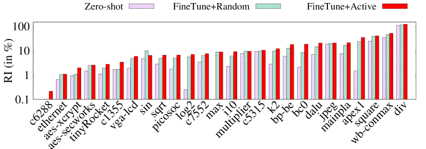
Table V shows the effectiveness of Bulls-Eye on large benchmarks ($\geq 40k$ nodes) where SOTA prior works do not work. We compared the QoR of synthesis output generated using recipes from SA $+$ Bulls-Eye as the back-end evaluator with our baselines. The results indicate high RI with respect to resyn2^∗ in reduction factor using recipes generated from Bulls-Eye predictors. Table VI shows runtime complexity and speedup of Bulls-Eye guided recipe generation. We present relative improvement and timing speedup of Bulls-Eye in Figure 6. We observe that $FT+A$-generated recipes achieve similar (and in one case significantly better) QoR with $\geq$ 2x run-time speed-up over $SA_{1k}$. $div$ achieved $>100\%$ RI compared to resyn2^∗ indicating that Bulls-Eye generated recipe optimized twice the number of nodes compared to resyn2 applied for the same time duration. Another crucial observation is: runtime speedup improves with more number of nodes in initial AIG. All designs having $\geq 10k$ nodes in initial AIG achieved more than 8x timing speed-up with similar QoR quality compared to $SA_{1k}$. To illustrate the faster recipe space search that comes from using Bulls-Eye QoR predictors, we chart the QoR progression over time in  Figure 7. The graphs show Bulls-Eye scales on large benchmarks and can generate superior quality synthesis recipes quickly compared to the conventional SA approach that uses actual synthesis runs. Note that the graph for $FT+A$ includes an initial time penalty from synthesis data generation and fine-tuning the model; after this the models enable very quick exploration of the recipe space due to fast inference by the proxy models.

((a)) bp_be

((b)) ethernet

((c)) jpeg

((d)) picosoc

((e)) tinyRocket

((f)) vga_lcd

((g)) wb_conmax

((h)) multiplier

Figure 7: QoR at various times from recipes by simulated annealing using different evaluators: actual synthesis ($B$) and proxy predictors ($ZS$ and $FT+A$)

VII Discussion and Insights

We proposed Bulls-Eye as a solution for ML-guided synthesis recipe generation that scales on large designs. Bulls-Eye uses few-shot learning and active learning to build upon models pre-trained on historical synthesis data, particularly given a limited synthesis run budget for new, unseen designs. Our framework generates better synthesis recipes compared to prior techniques, with an average $2.94$x run-time speed-up and up to $10.2$x speed-up (on large benchmarks) compared to conventional black-box approaches. We have made our code and associated dataset available to the community at: https://github.com/NYU-MLDA/OpenABC.

References

- [1] A. Mirhoseini et al., “A graph placement methodology for fast chip design,” Nature, vol. 594, no. 7862, pp. 207–212, 2021.
- [2] W. L. Neto et al., “LSOracle: a logic synthesis framework driven by artificial intelligence: Invited paper,” in ACM/IEEE International Conference on Computer-Aided Design, New York, NY, USA, 2019, pp. 1–6.
- [3] Y. Lin et al., “DREAMplace: Deep Learning Toolkit-Enabled GPU Acceleration for Modern VLSI Placement,” IEEE Transactions on Computer-Aided Design of Integrated Circuits and Systems, vol. 40, no. 4, pp. 748–761, 2020.
- [4] R. Brayton et al., “Abc: An Academic Industrial-Strength Verification Tool,” in International Conference on Computer Aided Verification. Berlin, Heidelberg: Springer, 2010, pp. 24–40.
- [5] C. Yu et al., “Developing synthesis flows without human knowledge,” in ACM/IEEE Design Automation Conference, New York, NY, USA, 2018, pp. 1–6.
- [6] A. Hosny et al., “DRiLLS: Deep reinforcement learning for logic synthesis,” in IEEE Asia South Pacific Design Automation Conference, New York, NY, USA, 2020, pp. 581–586.
- [7] K. Zhu et al., “Exploring logic optimizations with reinforcement learning and graph convolutional network,” in ACM/IEEE Workshop on Machine Learning for CAD, New York, NY, USA, 2020, pp. 145–150.
- [8] Y. V. Peruvemba et al., “Rl-guided runtime-constrained heuristic exploration for logic synthesis,” in ACM/IEEE International Conference On Computer Aided Design, New York, NY, USA, 2021, pp. 1–9.
- [9] W. Haaswijk et al., “Deep learning for logic optimization algorithms,” in IEEE International Symposium on Circuits and Systems, New York, NY, USA, 2018, pp. 1–4.
- [10] C. Yu, “Flowtune: Practical multi-armed bandits in boolean optimization,” in ACM/IEEE International Conference On Computer Aided Design, New York, NY, USA, 2020.
- [11] D. Silver, J. Schrittwieser, K. Simonyan, I. Antonoglou, A. Huang, A. Guez, T. Hubert, L. Baker, M. Lai, A. Bolton et al., “Mastering the game of go without human knowledge,” nature, vol. 550, no. 7676, pp. 354–359, 2017.
- [12] A. Krizhevsky, I. Sutskever, and G. E. Hinton, “Imagenet classification with deep convolutional neural networks,” Advances in neural information processing systems, vol. 25, pp. 1097–1105, 2012.
- [13] Y. Wang, Q. Yao, J. Kwok, and L. M. Ni, “Generalizing from a few examples: A survey on few-shot learning,” 2020.
- [14] A. B. Chowdhury, B. Tan, R. Karri, and S. Garg, “OpenABC-D: A large-scale dataset for machine learning guided integrated circuit synthesis,” 2021. [Online]. Available: https://github.com/NYU-MLDA/OpenABC
- [15] J. Deng et al., “ImageNet: A large-scale hierarchical image database,” in IEEE conference on computer vision and pattern recognition. New York, NY, USA: Institute of Electrical and Electronics Engineers, 2009, pp. 248–255.
- [16] Z. Bodó et al., “Active learning with clustering,” in Active Learning and Experimental Design workshop. JMLR Workshop and Conference Proceedings, 2011, pp. 127–139.
- [17] Y. Xiang et al., “Generalized simulated annealing algorithm and its application to the Thomson model,” Physics Letters A, vol. 233, no. 3, pp. 216–220, 1997.
- [18] “Opencores hardware RTL designs,” (https://opencores.org/).
- [19] “MIT Common Evaluation Platform(CEP),” (https://github.com/mit-ll/CEP), 2020.
- [20] J. Balkind, M. McKeown, Y. Fu, T. Nguyen, Y. Zhou, A. Lavrov, M. Shahrad, A. Fuchs, S. Payne, X. Liang et al., “OpenPiton: An open source manycore research framework,” ACM SIGPLAN Notices, vol. 51, no. 4, pp. 217–232, 2016.
- [21] T. Ajayi, D. Blaauw, T. Chan, C. Cheng, V. Chhabria, D. Choo, M. Coltella, S. Dobre, R. Dreslinski, M. Fogaça et al., “Openroad: Toward a self-driving, open-source digital layout implementation tool chain,” Proc. GOMACTECH, pp. 1105–1110, 2019.
- [22] S. Yang, Logic synthesis and optimization benchmarks user guide: version 3.0. Citeseer, 1991.
- [23] F. Brglez et al., “A neutral netlist of 10 combinational benchmark circuits and a target translator,” in IEEE International Symposium on Circuits and Systems, New York, NY, USA, 1985.
- [24] L. Amarú et al., “The EPFL combinational benchmark suite,” in IEEE International Workshop on Logic & Synthesis, New York, NY, USA, 2015.
- [25] xie jian jiang, “AES 128/256-bit symmetric block cipher,” (https://github.com/crypt-xie/XCryptCore/tree/master/ciphers/aes).
- [26] J. Strömbergson and O. Kindgren, “AES 128/256-bit symmetric block cipher,” (https://github.com/secworks/aes).
- [27] “Black Parrot SoC,” (https://github.com/black-parrot/black-parrot).
- [28] C. Albrecht, “IWLS 2005 benchmarks,” in IEEE International Workshop for Logic & Synthesis, New York, NY, USA, 2005.
- [29] F. Brglez, D. Bryan, and K. Kozminski, “Combinational profiles of sequential benchmark circuits,” in IEEE International Symposium on Circuits and Systems (ISCAS), 1989, pp. 1929–1934.