Bayesian Quantile Regression for Longitudinal Count Data
Abstract
This work introduces Bayesian quantile regression modeling framework for the analysis of longitudinal count data. In this model, the response variable is not continuous and hence an artificial smoothing of counts is incorporated. The Bayesian implementation utilizes the normal-exponential mixture representation of the asymmetric Laplace distribution for the response variable. An efficient Gibbs sampling algorithm is derived for fitting the model to the data. The model is illustrated through simulation studies and implemented in an application drawn from neurology. Model comparison demonstrates the practical utility of the proposed model.
keywords:
Asymmetric Laplace, Gibbs sampling, longitudinal count data, Markov chain Monte Carlo, Poisson process, quantile regression.1 Introduction
Research on count data models has accelerated following the work on multiple regression analysis of a Poisson process by [1]. The focus of successive literature lies on semiparametric estimation of conditional mean of count variables underneath pseudolikelihood framework. However, when the underlying response variable distribution is asymmetric, mean estimates become inadequate for inferences on the parameters of interest. This shortcoming prompted the research on fully parametric models describing the complete conditional distribution of parameters allowing to investigate the impact of the covariates on every aspect of the conditional distribution. Nonetheless, the strong parametric assumption and non-robust nature make these techniques unappealing.
More recent approach to the modeling and analyzing count data has involved the use of quantile regression techniques introduced by [2]. The central theme of their work is to estimate the conditional quantile functions. The idea of median regression involving minimization of sum of absolute residuals was introduced by Boscovich in the mid-18th century. The robustness of median regression over mean regression in the presence of even small number of outlying observations is discussed in literature at length, remarkably by Kolmogorov [3]. The commonplace assumption of Gaussian errors is often dubious and might result in surprising estimates of the coefficients of explanatory variables. Conversely, the quantile regression methods are able to handle the heteroscedasticity in the errors as well. A detailed guide on quantile regression and its properties is furnished by [4].
Various extensions to the quantile regression methods have been proposed in classical and Bayesian literature. Most of the developed techniques are primarily focused on continuous response data. The classical strand includes the simplex algorithm [5, 6, 7, 8, 9], the interior point algorithm [10, 11, 12], the smoothing algorithm [13, 14] and metaheuristic algorithms [15]. The crucial departure from continuous data setting in classical models was the work of [16, 17] for binary and multinomial models using median regression. Later, [18, 19] analyzed censored data using quantile regression, [20] studied median regression for discrete ordered responses and [21] gave quantile regression model for count data.
On the other hand, Bayesian quantile regression pivoted on Markov chain Monte Carlo (MCMC) methods employing asymmetric Laplace (AL) likelihoods was introduced by [22]. [23] proposed the normal-exponential mixture representation of the AL distribution and developed a Gibbs sampling algorithm. The AL likelihood has been used with or without the normal-exponential mixture to develop Bayesian estimation for quantile regression in Tobit models [24, 23], censored models [25], binary models [26, 27], count data models [28], ordinal models [29] and longitudinal data models [30, 31]. More recently, few works have emerged which propose Bayesian quantile regression analysis for discrete outcomes [32, 33, 34].
Moving on to the longitudinal data models, [35] presented penalization approach for the classical random effects estimator. In his model, an appropriate choice of degree of shrinkage or regularization term is required in order to control variability induced by random effects. Subsequently, likelihood based approach for quantile regression in longitudinal data models was proposed by [30] which makes use of AL density for likelihood to automate the choice of penalization level. They employed a Monte Carlo expectation maximization (EM) algorithm to estimate the model parameters. [31] made use of the normal-exponential mixture representation of AL density, presented in [23], to develop a random walk Metropolis Hastings (MH) algorithm and a Gibbs sampling algorithm for continuous longitudinal data. Furthermore, [36] and [37] used the similar framework to develop efficient Gibbs samplers for binary and ordinal longitudinal data respectively. Similarly, [38, 39] have fitted a Bayesian quantile regression joint model to ordinal and continuous longitudinal data and used Gibbs sampling for posterior inference. In this work, we propose a Bayesian quantile regression for longitudinal count data models employing the normal-exponential mixture for AL likelihood.
Longitudinal data models commonly arise in economics, finance, epidemiology, clinical trials and sociology. Some of these data may involve intensity of event recurrence at a given time as responses for each subject. Poisson distribution properly models such response variables most of the times. Aforesaid data is referred in literature as panel count data and predominantly observed in demographic studies, clinical trials and industrial reliability [40, 41, 42, 43, 44]. Effects of specific regressors on the underlying counting process are of practical importance in these regression analysis studies. Bayesian quantile regression approach to panel data is an active area of research and with this work we attempt to further the analysis of panel count data using Bayesian techniques.
Panel data involves repeatedly measured responses for independent subjects over time, hence serial correlation is naturally observed amongst the measures from the same subject. In such scenario, mixed models with random effects were popularized by [45]. Introduction of random effects to account for the within-subject variability avoids bias in parameter estimates, takes care of overdispersion in responses, and can assist in improving the model fit as well.
The rest of this paper is organized as follows. Section 2 introduces quantile regression and establishes relationship between quantile regression and asymmetric Laplace distribution. In Section 3, we discuss longitudinal count data models and their composition in terms of Bayesian quantile regression. This section also proposes a hierarchical Bayesian quantile regression model for longitudinal count data and introduces an efficient Gibbs sampling algorithm. Section 4 presents two Monte Carlo simulation studies and a real world application drawn from neurology. A brief discussion and conclusion is provided in Section 5. Technical derivations of conditional posterior densities are presented in the appendix.
2 Quantile Regression and Asymmetric Laplace Distribution
If we take and random variables and be the quantile level of the conditional distribution of , then a linear conditional quantile function is denoted as follows
| (1) |
where is the inverse cdf of conditional on and is a vector of unknown fixed parameters of length .
We consider the quantile regression approach for a linear model given by
| (2) |
where is the error term with pdf and is restricted to have its quantile to be zero.
Classical literature often does not mention the error density and estimation through quantile regression proceeds by minimizing the following objective function
| (3) |
where is the check function or quantile loss function defined by
here is an indicator function. This check function is not differentiable at zero, see Figure 1. Classical literature employs linear programming techniques such as the simplex algorithm, the interior point algorithm, the smoothing algorithm or metaheuristic algorithms to obtain quantile regression estimates for . The statistical programming language R makes use of quantreg package [46] to implement quantile regression techniques whilst confidence intervals are obtained via bootstrapping methods [4].

Median regression in Bayesian setting has been considered by [47] and [48]. In quantile regression, a link between maximum-likelihood theory and minimization of the sum of check functions, given in Equation 3, is provided by asymmetric Laplace distribution (ALD) [49, 22]. This distribution has location parameter , scale parameter and skewness parameter . Further details regarding the properties of this distribution are specified in [50]. If ALD, then its probability distribution function is given by
As discussed in [22], using the above skewed distribution for errors provides a way to cope the problem of Bayesian quantile regression effectively. According to them, any reasonable choice of prior, even an improper prior, generates a posterior distribution for . Subsequently, they made use of a random walk Metropolis Hastings algorithm with a Gaussian proposal density centered at the current parameter value to generate samples from analytically intractable posterior distribution of .
In the aforementioned approach, the acceptance probability depends on the choice of the value of , hence the fine tuning of parameters like proposal step size is necessary to obtain the appropriate acceptance rates for each . [23] overcame this limitation and showed that Gibbs sampling can be incorporated with AL density being represented as a mixture of normal and exponential distributions. Consider the linear model from Equation 2, where ALD, then this model can be written as
| (4) |
where, and are mutually independent, with N and represents exponential distribution. The and constants in the Equation 4 are given by
| (5) |
Consequently, a Gibbs sampling algorithm based on standard normal distribution can be implemented effectively. Currently, Brq [51] and bayesQR [52] are two R packages which provide Gibbs sampler for Bayesian quantile regression. We are exploiting the same technique to derive a Gibbs sampler for Bayesian quantile regression in longitudinal count data models.
3 Bayesian Quantile Regression for Longitudinal Count Data
3.1 Model Framework
Let be the repeated measurements data, for , where denotes the response measured for the th subject at th time and is row vector of a known design matrix . The response variables are counts and assumed to be generated via Poisson counting process. Poisson log-linear models have been typically used for such analyses and a general formulation is given by:
The longitudinal count data model can be expressed in the latent variable formulation as,
| (6) |
where denotes th latent variable for th individual, is vector of unknown fixed-effects parameters, is a row vector of covariates possessing random effects, is vector of unknown random-effects parameters and are the errors which are assumed to be and following ALD. Thus, the quantile level linear mixed quantile functions can be formulated in terms of a latent variable as given by
| (7) |
Latent variables in the above expression remain unobserved and only count variables are observed. [2] provided sufficient conditions for asymptotic inference of the parameters of stated in Equation 1. Among them, the continuity and positive support of the pdf of conditional on are the conditions of concern. Here, is generated through a counting process and its support is a set of nonnegative integers which does not satisfy both of the conditions specified. [21] dealt with this problem by jittering the variable with uniform noise to produce continuous variables. These jittered responses, , where unif, have continuous real valued quantiles and can be modeled as:
| (8) |
Models (7) and (8) are equivalent as we can obtain from through a monotonic transformation,
| (9) |
where, is a suitably small positive number. I take throughout this work. We can rewrite the Equation 8 as
To take into account the variation introduced by contamination of the count responses with uniformly distributed jittering variables, [21] applied their model to jittered data sets , for . They estimated the parameters of underlying regression as follows:
where, is the estimate obtained for a simulation on jittered response data . Instead of deriving expression for asymptotic covariance matrix, we can calculate the credible interval of average estimate by averaging the credible intervals of estimates, as given in [28]. The estimated conditional quantile function is specified as:
where, is the ceiling function. Now, we can give the complete data density of latent variables , conditional on , for and , with the assumption that they are identically and independently distributed according to the ALD.
In our case, the conditional quantile to be estimated, , is fixed and known beforehand. The random effects introduced here induce autocorrelation among the observations on the same subject. We assume that and terms are independent and further and are independent of each other.
Let and be the conditional density of latent response of subject conditional on the random effect . The complete latent data density of , for is given by
Let and , the joint latent data density of for N individuals is as follows:
| (10) |
3.2 The Hierarchical Model
After exploiting the normal-exponential mixture representation representing AL distribution and assuming the priors , we get the following hierarchical Bayesian quantile regression model:
| (11) | |||||
We can obtain the posterior distributions of parameters using the Bayes theorem in Equation 10 as follows:
Usually we are interested only in the inference regarding fixed-effects parameters which can be accomplished by obtaining the marginal distribution by integrating out the parameters from as given below
The next step in estimation is to choose appropriate prior distributions for each parameter. However, one needs to be cautious while selecting priors else issues can arise which could hamper the estimation and thereby inference process [53].
We have taken the normal prior, N, for the mutually indepedent random-effects parameters. As pointed out by [35], prior on has a penalty interpretation on the quantile loss function, and in my case, the normal prior implies penalization. penalization can be imposed by choosing an AL distribution as a prior [30]. One could set the prior to be N, but inference in such scenario becomes computationally expensive owing to the additional parameters to be estimated. Finally, we consider a hyper prior for , an inverse gamma (IG) distribution with shape parameter and scale parameter .
For the fixed-effects , the conventional choice of normal prior with zero mean leads to the ridge estimator. [54] showed that if differences in the size of fixed effects are large then the normal prior performs poorly. Instead we consider the Laplace prior for the fixed-effects, which takes the form as follows:
Laplace prior is a generalization of the ridge prior, which is equivalent to the Lasso model [55, 56]. The above prior can be written as given by [57],
Further the scale parameter is assigned a conjugate inverse gamma prior, IG, which allows it to be dynamically updated at each iteration in the Gibbs sampling algorithm. It removes the need to tune to obtain good acceptance rates such as in MCMC sampling using a Metropolis-Hastings algorithm.
Efficient values of parameters in an inverse-gamma prior have been debated a lot in the recent literature. The ordinary choice of shape and rate parameters to be each equal to 0.01 is widely criticized as it assigns negligible weight to small values of parameter on which prior beliefs are made. Following [58], we specify a flat prior on and with the shape parameter set to and rate parameter set to . It is nothing but an improper IG distribution which retains the conjugacy property of a proper IG distribution and at the same time remains vague in nature.
The joint posterior distribution of all parameters given the latent variable is formulated as given below:
where, , , , and . After substituting the probability distribution functions in the above equation it produces the following expression,
Where, and are the constants mentioned in the Equation 5 and is diagonal matrix with being the diagonal elements.
This joint posterior distribution does not possess a tractable form and Markov chain Monte Carlo simulation methods are used to carry out the Bayesian inference and eventually obtain the estimates of the parameters. Rather than sampling each component individually we consider within block sampling for similar to [31]. In their model, they sampled both fixed and random effects from their respective conditional posterior distributions in a linear mixed-effects model. This block sampling of parameters accounts for possible correlation among the components of and .
In within block sampling, we sample conditional on from an updated normal distribution and similarly is sampled conditional on from an another updated normal distribution. The latent variable is sampled from an updated generalized inverse Gaussian (GIG) distribution. The latent data variable is generated using the expression in Equation 9. In this process, jittering variables from uniform distribution are sampled at each iteration and utilized to obtain the latent variable whose conditional quantiles are continuous and hence can be modeled by a linear combination of covariates. The uniform jittering variables possess no practical importance and at each iteration new values are generated discarding the old ones. The parameters and are sampled from updated IG distributions. On the other hand, is sampled from an updated GIG distribution and is sampled from an updated gamma distribution. A detailed description of the Gibbs sampling algorithm is given below.
Algorithm
-
1.
Sample according to the Equation 9
-
2.
Sample for for and , where,
-
3.
Sample , where,
-
4.
Sample conditional upon from the distribution , where,
-
5.
Sample for , where, and .
-
6.
Sample , where, and .
-
7.
Sample conditional on from the distribution for , where,
-
8.
Sample , where, and .
4 Empirical Illustrations
4.1 Simulation Studies
4.1.1 Random Intercept Model
We considered the following simple linear mixed-effects model for latent variable formulation
| (12) |
where, number of subjects were 20 and for each subject number of repeated measurements were equal to 5. and were sampled independently from a uniform distribution on the interval and . A random intercept effect N was considered. As we don’t consider the fixed intercepts, the random intercepts account for them as well as the subject specific deviations. In this experiment, the counts were generated according to Poisson process. Hence, the counts were Poisson random variables with conditional mean given by
| (13) |
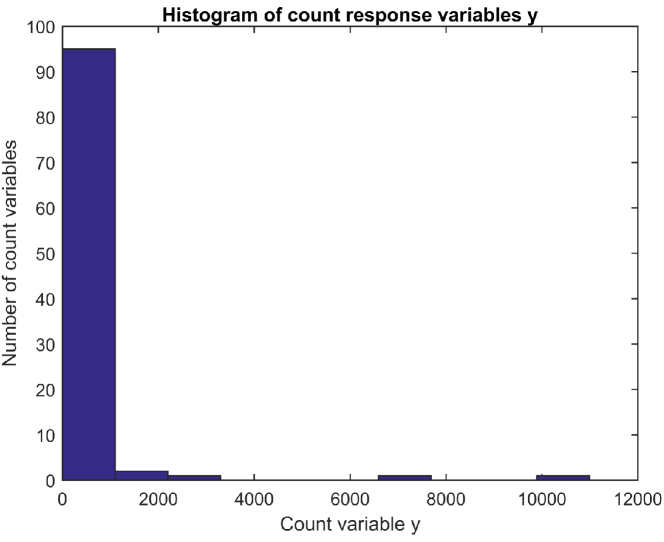
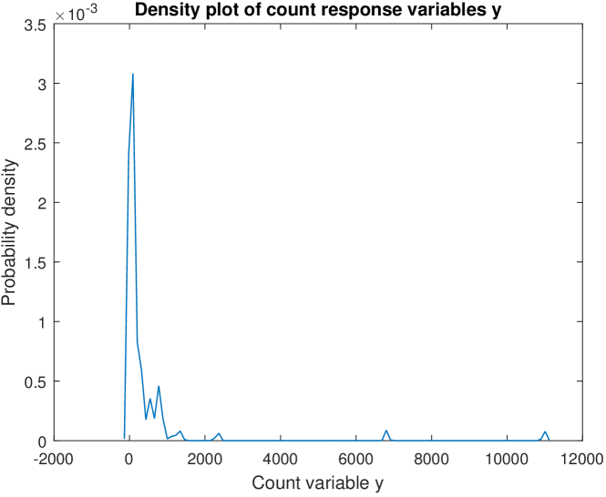
The histogram of count responses along with the smoothed kernel density plot is given in Figure 2. We then carried out Bayesian quantile regression at three different quantile levels, . We assumed weak prior information and assigned IG prior for as well as and considered Gamma prior on . To average out the noise added because of jittering, we implemented the average jittering estimator for each quartile with independent jittered data. According to [21], even with a moderate number of repetitions (say ) we can achieve high precision in average estimator as compared to a single posterior estimate. The Bayesian quantile regression using Gibbs sampling algorithm proposed above was run for r = 10000 iterations after initial 2000 iterations were discarded for burn-in on each jittered data.


The results for each quartile are presented in Table 1. We can see that the average posterior mean estimates for are close to the true parameter values. Standard deviations for these average estimators were calculated using the pooled variance technique given below. Average credible interval thus obtained was shorter than the credible interval of posterior mean for each jittered data revealing the improvement in precision of the average estimator.
| (14) | |||
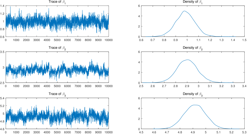
Trace plots and kernel density plots for and other hyperparameters at quantile regression are shown in Figure 3 and Figure 4 respectively. Convergence of chains for each parameter is observed through these trace plots which graphically demonstrate the appealing sampling achieved by our block sampling algorithm. Similar graphs were obtained for quantile regressions and can be made available on request.
To compare the Bayesian quantile regression models with the standard classical mean regression model, we performed random-effects Poisson regression (REPR) and results are presented in Table 2. We can see that coefficient values estimated are close to the true values and they are statistically significant as well. Our model gives average posterior means of the parameters close to their true values with slightly wider credible intervals in comparison to REPR model. Next, we calculated the negative log-likelihood (NLL) to compare the Bayesian quantile regression models with the classical model due to lack of a common information criterion across frequentist and Bayesian setting. The NLL for the REPR model was 398.5 and for our model the values for were 587.7, 390.7 and 417.7 respectively. This suggests that Bayesian quantile regression model fits the data better than any other model.
Furthermore, the model selection criterion such as deviance information criterion (DIC) [59, 60] proves helpful in choosing a value of which is most consistent with the data. The DIC values for and quartiles are 1878.8, 1142.7 and 1176.5 respectively. Hence, according to the DIC, median model provides the best fit among these three quantile regression models.
| Quantile | Par | True | Avg Post Mean | SD | Avg | Avg |
|---|---|---|---|---|---|---|
| 1 | 0.9981 | 0.1421 | 0.7039 | 1.2651 | ||
| 3 | 2.8788 | 0.1454 | 2.5829 | 3.1532 | ||
| 5 | 4.9470 | 0.1288 | 4.6892 | 5.1974 | ||
| 1 | 0.9856 | 0.0985 | 0.7899 | 1.1763 | ||
| 3 | 2.8957 | 0.1001 | 2.6947 | 3.0882 | ||
| 5 | 4.9506 | 0.0915 | 4.7694 | 5.1293 | ||
| 1 | 0.9708 | 0.0830 | 0.8064 | 1.1334 | ||
| 3 | 2.8790 | 0.0864 | 2.7101 | 3.0483 | ||
| 5 | 4.8970 | 0.0840 | 4.7332 | 5.0606 |
| Par | True | Coef | Std Err | 95% Conf Int | |
|---|---|---|---|---|---|
| 1 | 0.9360 | 0.0397 | 0.8581 | 1.0139 | |
| 3 | 2.9308 | 0.0416 | 2.8493 | 3.0124 | |
| 5 | 4.8937 | 0.0474 | 4.8009 | 4.9865 | |

4.1.2 Random Intercept and Slope Model
In this simulation study, we added a random slope term to the model (12). Therefore, the expression in (13) is modified as follows:
we sampled from unif(0,1) which is the covariate for random slope parameter. Other model specifications and priors are similar to the simulation study 1. The histogram of count response variables and the smoothed kernel density plot is shown in Figure 5. The Bayesian quantile regression using Gibbs sampling algorithm proposed above was run for 10000 iterations after initial 2000 burn-in iterations on each jittered data at each quartile.
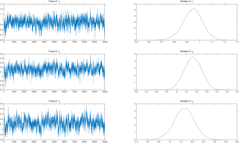
The results for each quantile regression model are presented in Table 3. Average posterior means for are close to the true values. Standard deviations were calculated according to the formula (14). Average credible intervals obtained were smaller in length than any of the individual credible intervals. Trace plots and kernel density plots for and hyperparameters are given below for quantile regression (see 6 and 7) Graphs at other quartiles can be made available on request. Inspection of trace plots suggests convergence of chains for each parameter and further validates the practical utility of our blocked procedure.
We also performed the mixed-effects Poisson regression (MEPR) to compare the Bayesian quantile regression models with the standard classical mean regression model. The results for MEPR model are given in Table 4. We can see that coefficient values estimated are close to the true parameter values and they are statistically significant as well. Our model results from Table 3 are competitive against this frequentist procedure with added benefit of data-driven uncertainty estimates. The NLL for the MEPR model was 464.4 and for the BQRLCD model the values for and quartiles are 800.5, 515.2 and 606.1 respectively. This shows that the MEPR model performs slightly better than Bayesian quantile regression models. The DIC values for quantile models were 2215.4, 1706.6 and 1821.5 respectively which implies that median model provides the best fit among these three quantile regression models.
| Quantile | Par | True | Avg Post Mean | SD | Avg | Avg |
|---|---|---|---|---|---|---|
| 1 | 0.9481 | 0.0848 | 0.7772 | 1.1088 | ||
| 3 | 3.1658 | 0.0903 | 2.9881 | 3.3396 | ||
| 5 | 5.1310 | 0.0978 | 4.9349 | 5.3165 | ||
| 1 | 0.9577 | 0.0656 | 0.8259 | 1.0850 | ||
| 3 | 3.1089 | 0.0773 | 2.9597 | 3.2612 | ||
| 5 | 5.0813 | 0.0847 | 4.9154 | 5.2474 | ||
| 1 | 0.9476 | 0.0582 | 0.8319 | 1.0618 | ||
| 3 | 3.0289 | 0.0717 | 2.8970 | 3.1748 | ||
| 5 | 5.0160 | 0.0824 | 4.8572 | 5.1785 |
| Par | True | Coef | Std Err | 95% Conf Int | |
|---|---|---|---|---|---|
| 1 | 1.0172 | 0.0305 | 0.9574 | 1.0771 | |
| 2 | 2.9969 | 0.0454 | 2.9080 | 3.0858 | |
| 3 | 5.0304 | 0.0469 | 4.9385 | 5.1224 | |

4.2 Progabide Clinical Trial Data Analysis
This section presents the application of Bayesian quantile regression for panel count data using the Progabide clinical trial data of 59 epileptic patients. Analyses on this data are reported in [61] and later in [62].
Patients with partial seizures were enrolled in a randomized clinical trial of Progabide, an anti-epileptic drug. Participants in the study were randomized to either Progabide/treatment or a placebo/control group, as a chemotherapy adjuvant. Progabide is an anti-epileptic drug and its principal course of action is to improve the gamma-aminobutyric acid (GABA) content. GABA is the primary inhibitory neurotransmitter in the brain. Prior to receiving the treatment, baseline seizure count data on the number of epileptic seizures during the preceding 8-week interval were recorded. At each of four successive post-randomization visits, number of seizures occurring over past 2 weeks was recorded. Although subsequently each patient was crossed over to the other treatment, we have only taken into consideration the pre-crossover responses. The seizure count data exhibits high dispersion, heteroscedasticity, and serial correlation for each patient. Histogram plot and kernel density plot of biweekly seizure counts are given in Figure 8.


We have specified the descriptive statistics of the response variable in Table 6. We found that the patient with ID = 49 possessed very high baseline as well as the post-randomization seizure counts. Omitting this patient lead to a significant drop in the mean, standard deviation, and correlations of Progabide group. But, this deletion of a patient had no clinical ground and only the prediction purpose was being served. The dispersion as well as the within subject dependence were still at a significant level even after the removal of outlier.
We considered two longitudinal count data models. The regressors taken in these two models included baseline seizure rate, computed as the natural log of quarter of 8-week pre-randomization seizure count (Base), natural logarithm of age (LnAge), treatment indicator variable for the Progabide group (Trt), last visit indicator variable for the fourth visit to the clinic (Visit) and an interaction term of treatment indicator and baseline seizure count (Base.Trt). The visit indicator variable is added owing to the previous studies showing a significant decrease in the seizures prior to the fourth clinical visit. These variables are a part of larger collection of explanatory variables which were not present in the dataset we retrieved. Selected variables are in-line with the previous literature on the regression analysis of the given data.
| Group | Variables | Mean | Median | Min | Max | SD |
| Placebo | Age | 28.96 | 29 | 19 | 40 | 5.40 |
| (28 Subjects) | Baseline Seizure Count | 30.79 | 19 | 6 | 111 | 25.63 |
| Progabide | Age | 28.71 | 26 | 18 | 57 | 8.79 |
| (31 Subjects) | Baseline Seizure Count | 31.65 | 24 | 7 | 151 | 27.54 |
| Progabide | Age | 28.93 | 26 | 18 | 57 | 8.85 |
| (30 Subjects - | Baseline Seizure Count | 27.67 | 23 | 7 | 76 | 17.12 |
| Outlier removed) |
| Placebo (28 subjects) | Progabide (31 subjects) | |||||||||||
| Visit | Mean | SD | Correlations | Mean | SD | Correlations | ||||||
| 1 | 9.36 | 9.95 | 1.00 | 8.58 | 17.94 | 1.00 | ||||||
| 2 | 8.29 | 8.02 | 0.78 | 1.00 | 8.42 | 11.67 | 0.91 | 1.00 | ||||
| 3 | 8.79 | 14.41 | 0.51 | 0.66 | 1.00 | 8.13 | 13.67 | 0.91 | 0.92 | 1.00 | ||
| 4 | 8.00 | 7.47 | 0.67 | 0.78 | 0.68 | 1.00 | 6.74 | 11.07 | 0.97 | 0.95 | 0.95 | 1.00 |
| Progabide (30 Subjects - outlier removed) | ||||||
| Visit | Mean | SD | Correlations | |||
| 1 | 5.47 | 5.67 | 1.00 | |||
| 2 | 6.53 | 5.51 | 0.45 | 1.00 | ||
| 3 | 6.00 | 7.25 | 0.63 | 0.70 | 1.00 | |
| 4 | 4.87 | 4.20 | 0.77 | 0.72 | 0.83 | 1.00 |
We considered random intercept model (model-1) and random intercept with random visit effects model (model-2). We added random effects for the visit indicator as it is a time-varying variable and hence the coefficients on these effects present the subject specific deviations due to the fourth clinic visit. Also, these models were crosschecked for performance with their standard classical counterparts which are the REPR and the MEPR with random visit effects respectively. Priors on the parameters and hyperparameters were same as that specified in the simulation studies. Table 8 reports the estimates with their standard deviation for 2 models in Bayesian framework obtained from 10000 iterations after initial burn-in of 2000 iterations. On the other hand, the REPR and the MEPR model parameter estimates, their standard errors and p-values are given in Table 9 and Table 10 respectively.
The coefficient values of all the regressors except the base and visit variables are statistically insignificant at 5% significance level for the REPR model. Whereas, in the MEPR model with random visit effects, only the base variable is statistically significant. In the Bayesian setting, besides the base variable, all other variables cannot be differentiated from 0 according to their credible intervals. We observed that random intercept accounted for significant amount of variability in the REPR and the MEPR model. However, there was less unobserved subject specific variability for the visit indicator variable.
The interaction variable between the treatment and the baseline seizure rate produces interesting results for the classical REPR model. The mean seizure rate for the Progabide group maybe higher or lower than the placebo group depending upon the baseline seizure rate. This indicates contraindication for patients with higher rate of seizures. For other models, due to lack of statistical significance commenting on this phenomenon is irrelevant.
Finally for model comparison among Bayesian and classical models, NLL values were calculated using the estimates of coefficients. The NLL value for the REPR model was 645.6 and for the model-1 NLL values for and quartiles were 1044, 789.6 and 692.6 respectively. This indicates that the our method has comparative performance against well established REPR model. Furthermore, the DIC values obtained for these Bayesian models were 2215.5, 1697.8 and 1660.7 respectively which highlights that quantile model provides the best fit among these three quantile regression models.
Similar model comparisons were performed for second modeling scenario. The NLL for the MEPR model with random visit effects was 639.8 and for our three Bayesian quartile models the NLL values were 1048.7, 798.4 and 730.4 for , and quartiles respectively. This again shows that the classical regression model (MEPR in this case) slightly outperforms the best performing Bayesian model. Nonetheless, a frequentist model can be overly confident about its predictions as well as they lack the ability to quantify uncertainty associated with their estimates. Next, the DIC values were 2234.7, 1694.8 and 1702.3 for , and Bayesian quartile models which suggests that median and the quantile models fit the data similarly well.
| Model | Variables | 25th Quartile | 50th Quartile | 75th Quartile | |||
|---|---|---|---|---|---|---|---|
| Mean | SD | Mean | SD | Mean | SD | ||
| Model-1 | Intercept | -0.1462 | 0.4934 | -0.0634 | 0.3672 | 0.0322 | 0.3693 |
| Base | 0.8671 | 0.1720 | 0.9100 | 0.1049 | 0.8901 | 0.1025 | |
| Trt | -0.4409 | 0.4153 | -0.2534 | 0.2625 | -0.2259 | 0.2553 | |
| LnAge | -0.0124 | 0.1560 | 0.0698 | 0.1152 | 0.1410 | 0.1167 | |
| Visit | -0.0222 | 0.1883 | -0.0048 | 0.1184 | -0.0512 | 0.1030 | |
| Base.Trt | 0.0118 | 0.2023 | -0.0561 | 0.1351 | -0.0314 | 0.1323 | |
| Model-2 | (Visit RE) | ||||||
| Intercept | -0.1475 | 0.4990 | -0.0763 | 0.3882 | 0.0069 | 0.3672 | |
| Base | 0.8720 | 0.1710 | 0.9125 | 0.1028 | 0.8891 | 0.0949 | |
| Trt | -0.4275 | 0.4003 | -0.2556 | 0.2543 | -0.2159 | 0.2395 | |
| LnAge | -0.0139 | 0.1546 | 0.0730 | 0.1201 | 0.1477 | 0.1166 | |
| Visit | -0.0421 | 0.1929 | -0.0094 | 0.1220 | -0.0392 | 0.1133 | |
| Base.Trt | 0.0043 | 0.1998 | -0.0565 | 0.1321 | -0.0274 | 0.1255 | |
| Variables | Coef | Std Err | p-value |
|---|---|---|---|
| Intercept | -0.9362 | 1.0666 | 0.380 |
| Base | 0.8909 | 0.1297 | 0.000 |
| Trt | -0.6410 | 0.4181 | 0.125 |
| LnAge | 0.3602 | 0.3098 | 0.245 |
| Visit | -0.1425 | 0.0590 | 0.016 |
| Base.Trt | 0.1562 | 0.2166 | 0.471 |
| Variables | Coef | Std Err | p-value |
|---|---|---|---|
| Intercept | -0.9951 | 0.9964 | 0.318 |
| Base | 0.9032 | 0.1184 | 0.000 |
| Trt | -0.5964 | 0.3972 | 0.133 |
| LnAge | 0.3684 | 0.2893 | 0.203 |
| Visit | -0.0598 | 0.0782 | 0.568 |
| Base.Trt | 0.1150 | 0.2011 | 0.568 |
5 Conclusion
In this paper, we present a Bayesian quantile regression model for longitudinal count data and derive an efficient MCMC - Gibbs sampling algorithm to estimate the proposed model. This model makes use of latent variable formulation of count response data and the estimation procedure exploits the normal-exponential mixture representation of asymmetric Laplace density. The developed framework contributes to the literature on quantile regression for discrete data, panel data models for quantile regression, and discrete longitudinal/panel data models. Furthermore it has potential application in the fields like epidemiology, economics and business. One attractive feature our work lies in the robustness of the proposed model which requires minimal assumptions on the distribution of errors allowing for skewed, heavy-tailed distributions for errors as well as accommodation of outliers. The empirical illustrations provided in the paper demonstrate the computational efficiency of the estimation algorithm and the blocking approach.
References
- [1] Jorgenson DW. Multiple regression analysis of a poisson process. Journal of the American Statistical Association. 1961;56:235–245.
- [2] Koenker R, Basset G. Regression quantiles. Econometrica. 1978;46:33–50.
- [3] Shiryayev AN. The method of the median in the theory of errors. In: Shiryayev AN, editor. Selected works of a. n. kolmogorov: Volume ii probability theory and mathematical statistics. Springer Netherlands, Dordrecht; 1992. p. 115–117.
- [4] Koenker R. Quantile regression. 1st ed. Cambridge University Press, Cambridge; 2005.
- [5] Dantzig GB. Linear programming and extensions. Princeton University Press, Princeton; 1963.
- [6] Dantzig GB, Thapa MN. Linear programming 1: Introduction. Springer, New York; 1997.
- [7] Dantzig GB, Thapa MN. Linear programming 2: Theory and extensions. Springer, New York; 2003.
- [8] Barrodale I, Roberts F. Improved algorithm for discrete linear approximation. SIAM Journal of Numerical Analysis. 1973;10(5):839–848.
- [9] Koenker R, d’Orey V. Computing regression quantiles. Journal of the Royal Statistical Society - Series C (Applied Statistics). 1987;36(3):383–393.
- [10] Karmarkar N. A new polynomial time algorithm for linear programming. Combinatorica. 1984;4(4):373–395.
- [11] Mehrotra S. On the implementation of primal-dual interior point methods. SIAM Journal of Optimization. 1992;2(4):575–601.
- [12] Portnoy S, Koenker R. The gaussian hare and laplacian tortoise: computability of squared-error versus absolute-error estimators. Statistical Science. 1997;12(4):279–300.
- [13] Madsen K, Nielsen HB. A finite smoothing algorithm for linear estimation. SIAM Journal of Optimization. 1993;3:223–235.
- [14] Chen C. A finite smoothing algorithm for quantile regression. Journal of Computational and Graphical Statistics. 2007;16:136–164.
- [15] Rahman MA. Quantile regression using metaheuristic algorithms. International Journal of Computational Economics and Econometrics. 2013;3:205–233.
- [16] Manski CF. Maximum score estimation of the stochastic utility model of choice. Journal of Econometrics. 1975;3:205–228.
- [17] Manski CF. Semiparametric analysis of discrete response: asymptotic properties of the maximum score estimator. Journal of Econometrics. 1985;27:313–333.
- [18] Powell JL. Least absolute deviation estimation for the censored regression model. Journal of Econometrics. 1984;25:303–325.
- [19] Powell JL. Censored regression quantiles. Journal of Econometrics. 1986;32:143–155.
- [20] Lee MJ. Median regression for ordered discrete response. Journal of Econometrics. 1992;51:59–77.
- [21] Machado J, Santos Silva J. Quantiles for counts. Journal of the American Statistical Association. 2005;100:1226–1237.
- [22] Yu K, Moyeed R. Bayesian quantile regression. Statistics and Probability Letters. 2001;54(4):437–447.
- [23] Kozumi H, Kobayashi G. Gibbs sampling methods for bayesian quantile regression. Journal of Statistical Computation and Simulation. 2011;81:1565–1578.
- [24] Yu K, Stander J. Bayesian analysis of a tobit quantile regression model. Journal of Econometrics. 2007;137:260–276.
- [25] Reich BJ, Smith LB. Bayesian quantile regression for censored data. Biometrics. 2013;69:651–660.
- [26] Hewson P, Yu K. Quantile regression for binary performance indicators. Appl Stochastic Models Bus Ind. 2008;24(5):401–418.
- [27] Benoit DF, Poel DVD. Binary quantile regression: a bayesian approach based on the asymmetric laplace distribution. Journal of Applied Econometrics. 2010;27:1174–1188.
- [28] Lee D, Neocleous T. Bayesian quantile regression for count data with application to environmental epidemiology. Journal of the Royal Statistical Society: Series C (Applied Statistics). 2010;59(5):905–920.
- [29] Rahman MA. Bayesian quantile regression for ordinal models. Bayesian Analysis. 2016;11:1–24.
- [30] Geraci M, Bottai M. Quantile regression for longitudinal data using the asymmetric laplace distribution. Biostatistics. 2007;8:140–154.
- [31] Luo Y, Lian H, Tian M. Gibbs sampling methods for bayesian quantile regression. Journal of Statistical Computation and Simulation. 2012;82:1635–1649.
- [32] Rahman MA., Karnawat S. Flexible Bayesian Quantile Regression in Ordinal Models. Advances in Econometrics. 2019;40B:211–251.
- [33] Alhamzawi R., Ali HTM. Bayesian single-index quantile regression for ordinal data. Communications in Statistics - Simulation and Computation. 2020;49:1306–1320.
- [34] Bresson G., Lacroix G., Rahman MA. Bayesian panel quantile regression for binary outcomes with correlated random effects: an application on crime recidivism in Canada. Empirical Economics. 2021;60:227–259.
- [35] Koenker R. Quantile regression for longitudinal data. Journal of Multivariate Analysis. 2004;91:74–89.
- [36] Rahman MA, Vossmeyer A. Estimation and applications of quantile regression for binary longitudinal data. Advances in Econometrics. 2019;40B:157–191.
- [37] Alhamzawi R, Ali HTM. Bayesian quantile regression for ordinal longitudinal data. Journal of Applied Statistics. 2018;45(5):815–828. Available from: https://doi.org/10.1080/02664763.2017.1315059.
- [38] Ghasemzadeh S, Ganjali M, Baghfalaki T. A Bayesian conditional model for bivariate mixed ordinal and skew continuous longitudinal responses using quantile regression. Journal of Applied Statistics. 2018;45:2619–2642. Available from: https://doi.org/10.1080/02664763.2018.1431208.
- [39] Ghasemzadeh S, Ganjali M, Baghfalaki T. Bayesian quantile regression for joint modeling of longitudinal mixed ordinal and continuous data. Communications in Statistics - Simulation and Computation. 202049:375–395. Available from: https://doi.org/10.1080/03610918.2018.1484482.
- [40] Kalbfleisch JD, Lawless JF. The analysis of panel data under a markov assumption. Journal of the American Statistical Association. 1985;80:863–871.
- [41] Gaver DP, O’Muircheartaigh I. Robust empirical bayes analyses of event rates. Technometrics. 1987;29:1–15.
- [42] Thall PF, Lachin JM. Nonparametric methods for random-interval count data. Journal of the American Statistical Association. 1988;83:339–347.
- [43] Thall PF. Mixed poisson likelihood regression models for longitudinal interval count data. Biometrics. 1988;44:197–209.
- [44] Sun J, Kalbfleisch JD. The analysis of panel data under a markov assumption. Statistica Sinica. 1995;5:279–289.
- [45] Laird NM, Ware JH. Random-effects models for longitudinal data. Biometrics. 1982 Dec;38(4):963–974.
- [46] Koenker R. Package ‘quantreg’ [https://cran.r-project.org/web/packages/quantreg/quantreg.pdf]; 2017. [Online; accessed 1-May-2017]”.
- [47] Walker SG, Mallick BK. A bayesian semiparametric accelerated failure time model. Biometrics. 1999;55:477–483.
- [48] Kottas A, Gelfand AE. Bayesian semiparametric median regression modeling. Journal of the American Statistical Association. 2001;96:1458–1468.
- [49] Koenker R, Machado J. Goodness of fit and related inference processes for quantile regression. Journal of the American Statistical Association. 1999;94:1296–1309.
- [50] Yu K, Zhang J. A three-parameter asymmetric laplace distribution and its extensions. Communications in Statistics- Theory and Methods. 2005;34:1867–1879.
- [51] Alhamzawi R. Package ‘brq’ [https://cran.r-project.org/web/packages/Brq/Brq.pdf]; 2017.
- [52] Benoit DF, Alhamzawi R, Yu K, et al. Package ‘bayesqr’ [https://cran.r-project.org/web/packages/bayesQR/bayesQR.pdf]; 2017.
- [53] Kinney SK, Dunson DB. Fixed and random effects selection in linear and logistic models. Biometrics. 2007;63(3):690–698.
- [54] Griffin J, Brown PJ. Inference with normal-gamma prior distributions in regression problems. Bayesian Analysis. 2010;5(1):171–188.
- [55] Tibshirani R. Regression shrinkage and selection via the lasso. the Royal Statistical Society Series B (Methodological). 1996;58(1):267–288.
- [56] Bae K, Mallick BK. Gene selection using a two-level hierarchical bayesian model. Bioinformatics. 2004;20(18):3423–3430.
- [57] Andrews DF, Mallows CL. Scale mixtures of normal distributions. Journal of the Royal Statistical Society Series B (Methodological). 1974;36(1):99–102.
- [58] Gelman A. Prior distributions for variance parameters in hierarchical models. Bayesian Analysis. 2006;1:515–533.
- [59] Spiegelhalter DJ, Best NG, Carlin BP, et al. Bayesian measures of model complexity and fit. Journal of the Royal Statistical Society – Series B (Statistical Methodology). 2002;64(4):583–639.
- [60] Celeux G, Forbes F, Robert CP, et al. Deviance information criteria for missing data models. Bayesian Analysis. 2006;1(4):651–674.
- [61] Leppik IE, et al. A double-blind crossover evaluation of progabide in partial seizures. Neurology. 1985;35:285.
- [62] Thall PF, Vail SC. Some covariance models for longitudinal count data with overdispersion. Biometrics. 1990;46:657–671.
Appendix A Conditional Densities of the Parameters for Gibbs Sampler
In the proposed model, the full conditional posterior densities of all the parameters presented in the Gibbs sampling algorithm except the latent data variable are derived from the complete posterior density expression exhibited in Equation 10. From the full hierarchical Bayesian quantile regression model, we get
where, and are defined in Equation 5. The above density expression for an individual can be identified as the kernel of a generalized inverse Gaussian distribution GIG, where, and,
The full conditional posterior distribution of denoted by is
That is the kernel of an inverse gamma distribution with the and parameters given by
The full conditional distribution of is given as follows:
where in the third line we collect the terms involving parameter and the successive line introduces two new terms, and , which are stated as follows,
where, is the matrix. Adding and subtracting inside the square brackets in the last line of the derivation of distribution of helps in completing the square.
As does not involve and can be omitted as it gets included in the proportionality constant. The result can be recognized as the kernel of a Gaussian distribution and therefore N.
The full conditional distribution of each , denoted by is given by
Thus, the above density expression of can be recognized as the kernel of a generalized inverse Gaussian distribution, GIG, where and .
The full conditional distribution of which is denoted by is
It is clear that the above expression is the kernel of a Gamma distribution, where,
Th full conditional posterior distribution of is given by
where, in the third line we omit terms which do not include parameter and on the next line we introduce two new terms, and , which are defined below,
where, is the matrix. Adding and subtracting inside the curly braces in the last line of the derivation of distribution of helps in completing the square.
As does not involve and can be omitted as it gets included in the proportionality constant. The result can be recognized as the kernel of a Gaussian distribution and therefore N.
The full conditional posterior distribution of denoted by is
That is the kernel of an inverse gamma distribution with the (shape) and (scale) parameters given as follows: