Two years of optical and NIR observations of the superluminous supernova UID 30901 discovered by the UltraVISTA SN survey

Abstract

We present deep optical and near-infrared photometry of UID 30901, a superluminous supernova (SLSN) discovered during the UltraVISTA survey. The observations were obtained with VIRCAM ($YJHK_{s}$) mounted on the VISTA telescope, DECam ($griz$) on the Blanco telescope, and SUBARU Hyper Suprime-Cam (HSC; $grizy$). These multi-band observations comprise +700 days making UID 30901 one of the best photometrically followed SLSNe to date. The host galaxy of UID 30901 is detected in a deep HST F814W image with an AB magnitude of $27.3\pm 0.2$. While no spectra exist for the SN or its host galaxy, we perform our analysis assuming $z=0.37$, based on the photometric redshift of a possible host galaxy found at a projected distance of 7 kpc. Fitting a blackbody to the observations, the radius, temperature, and bolometric light curve are computed. We find a maximum bolometric luminosity of $5.4\pm 0.34\times 10^{43}$ erg s^-1. A flattening in the light curve beyond 600 days is observed and several possible causes are discussed. We find the observations to clearly favour a SLSN type I, and plausible power sources such as the radioactive decay of ⁵⁶Ni and the spin-down of a magnetar are compared to the data. We find that the magnetar model yields a good fit to the observations with the following parameters: a magnetic field $B=1.4\pm 0.3\times 10^{14}$ G, spin period of $P=6.0\pm 0.1$ ms and ejecta mass $M_{ej}=11.9^{+4.8}_{-6.4}M_{\odot}$.

1 Introduction

Two decades ago a new kind of extremely bright stellar explosion was uncovered, now known as superluminous supernovae (SLSNe). These objects are rare and can often reach absolute magnitudes of $M\sim-21$ at maximum light (Gal-Yam, 2019). It was soon realised that some of these SNe exhibit hydrogen in their spectra, while others do not, giving as a result Type II and Type I SLSNe sub-classes (Gal-Yam, 2012) respectively, in analogy with normal luminosity SNe (see Filippenko, 1997).

Hydrogen-poor SLSNe are generally characterised by a very blue, nearly featureless optical spectrum, a lack of hydrogen lines and the display of characteristic O ii absorption lines near maximum light. The presence of O ii absorption lines is a signature of the high temperature and ionisation state of the SN ejecta at early times (e.g, Mazzali et al., 2016). A few weeks after maximum, when the ejecta has cooled enough, their spectra become similar to SNe Ic (Pastorello et al., 2010) or to broad-line Ic SNe (Ic-Bl Liu et al., 2017).

After a few hundred days, their nebular spectra are dominated by intermediate mass elements, resembling SNe Ic-BL (Milisavljevic et al., 2013; Nicholl et al., 2016b; Jerkstrand et al., 2017; Nicholl et al., 2019). Recently, it has been noted that hydrogen poor SLSNe span a wide range in peak luminosities ($-22\lesssim M_{g}\lesssim-20$ mag), overlapping with the Ic-BL SN class (De Cia et al., 2018). However, while some degree of similarity exists between SLSNe-i and Ic/Ic-BL, De Cia et al. (2018) and Quimby et al. (2018) have recently claimed that hydrogen-poor SLSNe are both photometrically and spectroscopically a distinct SN class.

Hydrogen-rich or Type II SLSNe are less common objects than SLSNe-I, and are characterised by a distinctive H$\alpha$ emission line. There is large diversity in the observational signatures of hydrogen-rich SLSNe. In this class, we find objects such as SN 2006gy (Smith et al., 2007; Ofek et al., 2007) which are presumed to be powered by strong SN ejecta circumstellar medium (CSM) interaction. These kinds of SLSNe display narrow and broad H$\alpha$ emission components, which are characteristic of Type IIn SNe (Schlegel, 1990). Objects such as SN 2006gy are frequently considered the bright end of the Type IIn class. Among SLSNe-II, we can also find objects such as SN 2008es (Miller et al., 2009; Gezari et al., 2009), displaying a very blue and featureless continuum at early times, no O ii lines or narrow lines in the spectra, but developing a strong and broad dominant H$\alpha$ feature after a few days. The interaction between the SN ejecta with a dense CSM is less evident in objects like SN 2008es, but maybe the main power source. The diversity of the SLSNe-II class was further characterised through two objects reported by Inserra et al. (2018).

There is an interesting subset of objects initially classified as SLSNe-I, such as iPTF16bad and iPTF13ehe (Yan et al., 2015, 2017), which show broad H$\alpha$ emission after maximum light and signatures of SN ejecta-CSM interaction. These objects suggest ejections of hydrogen-rich material shortly before the SN explosion. These mass ejections may be more common in SLSNe-I than currently detected, although radio (Nicholl et al., 2016b) and X-ray (Margutti et al., 2018) observations favour low density environments similar to SNe Ic. However, due to the high redshifts at which SLSNe are frequently found, it is often difficult to secure high signal-to-noise observations in X-rays, radio, or in the optical/NIR at late times to place strong constraints on the environment surrounding the SN.

In the last decade, several researchers have proposed diverse physical mechanisms to power the extreme luminosity of SLSNe. They can be summarised as: 1) the interaction between a fast SN ejecta and a dense CSM that transforms the ejecta kinetic energy into thermal energy, 2) the radioactive decay of several solar masses of ⁵⁶Ni synthesised during the SN explosion and 3) the power injection from a central engine such as fallback accretion onto a black hole (Dexter & Kasen, 2013) or a rapidly rotating neutron star with a strong magnetic field -a magnetar- formed during the core collapse (Woosley, 2010; Kasen & Bildsten, 2010).

Most SLSNe-II exhibit hydrogen signatures and light curves with maximum luminosity, duration, shape and decline rate that seem to be well explained within the context of ejecta-CSM interaction models. An example of this is the analytical ejecta-CSM interaction model implemented by Chatzopoulos et al. (2013) which can reproduce most of the diversity exhibited by the light curves of this type of event. This model assumes that the progenitor star is surrounded by a CSM shell described by a power law density profile $\rho_{\mathrm{CSM}}=qr^{-s}$, where 0 or 2 are physically motivated values for $s$. The first value describes a shell of constant density and the latter a steady-wind. However, we have to consider that simple analytical models although powerful to obtain an estimate of CSM properties, are not able to capture the full complexity of the ejecta-CSM interaction (see e.g., Moriya et al., 2018). For example, the pre-SN mass loss history can be more complex resulting in CSM clumps or shells, with non-spherical distributions, resulting in a diverse set of SN light curves and spectra, depending on the viewing angle which may, in part, explain the observational diversity observed in SLSNe-II.

In the case of SLSN-I, however, the power source is less clear. One possibility is that their extreme luminosity can be due to ejecta-CSM interaction as in SLSNe-II, but in this case considering a fast SN ejecta with a hydrogen and helium poor CSM (see Moriya et al., 2018, for a review). The handful objects initially classified as SLSNe-I at early times, but later showing broad H$\alpha$ emission and other signatures of CSM-ejecta interaction (Yan et al., 2015, 2017), may bridge the gap between SLSNe-I and SLSNe-II populations. However, several challenges remain for the interaction model to explain the SLSN-I population. For example, whether it is possible for a massive star to expel large enough quantities of hydrogen-free material to power SLSNe light curves through an ejecta-CSM interaction. Another important question for this scenario is whether the spectral features observed in SLSNe-I can be produced by ejecta-CSM interaction. It is important to consider that several days after maximum light SLSNe-I spectra resemble non-interacting stripped envelope core collapse SNe (Ic and Ic-BL), suggesting that strong interaction does not play a role in the formation of the spectral features in SLSNe-I.

A different route to power SLSNe is through the radioactive decay of several solar masses of ⁵⁶Ni synthesised in a Pair Instability SN (Gal-Yam et al., 2009; Kasen et al., 2011). In the exceptional instance of stars born in low metallicity environments with a main-sequence mass in the range 140-260 $M_{\odot}$ (Heger & Woosley, 2002), an instability due to the production of positron-electron pairs can lead to a thermonuclear explosion (Barkat et al., 1967; Rakavy & Shaviv, 1967), known as a PISN.

PISNe are predicted to ejecta several solar masses of ⁵⁶Ni. Its radioactive decay products and other iron-peak elements should produce: 1) strong blanketing below $\sim 4000$ Å shifting the peak of the spectral energy distribution (SED) towards redder wavelengths (Dessart et al., 2012), and 2) a nebular spectrum dominated by emission lines from iron-peak elements (Dessart et al., 2012; Jerkstrand et al., 2016; Mazzali et al., 2019). These signatures of PISN are in stark contrast with the characteristics displayed by SLSNe-I, which: 1) exhibit a very blue SED before and around maximum light, peaking below $4000$ Å, and 2) have nebular spectra dominated by emission lines from intermediate-mass elements (Milisavljevic et al., 2013; Jerkstrand et al., 2017; Nicholl et al., 2019; Mazzali et al., 2019).

A popular model that can reproduce the high luminosities observed in SLSNe-I, invokes the spin-down of a fast rotating and highly magnetic neutron star, that energizes the SN ejecta (Woosley, 2010; Kasen & Bildsten, 2010). Using a small sample of well-observed hydrogen poor SLSNe, Inserra et al. (2013) discarded the decay of ⁵⁶Ni as the power source for their objects and instead showed that the energy injection from the spin-down of a magnetar can successfully reproduce the complete light curve evolution, including their flattening at late times. More recently, Nicholl et al. (2017) presented a sophisticated version of the magnetar model built-in the Modular Open Source Fitter for Transients (Guillochon et al., 2018, MOSFiT), which they fit to a large sample of hydrogen poor SLSNe collected from the literature to show that this model can successfully explain the light curve evolution of this SN class.

The characterisation of SLSNe host galaxies also plays an important role in constraining their possible progenitors. Several studies have shown that SLSNe-I have a strong preference for low mass dwarf galaxies ($M_{\mathrm{stellar}}<10^{9}M_{\odot}$) (Neill et al., 2011; Lunnan et al., 2014; Leloudas et al., 2015; Angus et al., 2016; Perley et al., 2016; Schulze et al., 2018), with metallicity usually below 0.5  Z_☉ (Lunnan et al., 2014; Leloudas et al., 2015; Perley et al., 2016; Schulze et al., 2018) and high specific star formation rates (Neill et al., 2011; Lunnan et al., 2014; Perley et al., 2016). On the other hand, SLSNe-II seems to explode in a wider range of environments, from the extreme environments typical of SLSNe-I to those of normal luminosity core collapse SNe (Leloudas et al., 2015; Perley et al., 2016; Schulze et al., 2018).

In this paper, we present and analyse $YJHK_{s}$ photometry of UID 30901 spanning more than 700 days of observations from the UltraVISTA survey. UltraVISTA is a deep near-infrared (NIR) galaxy survey, running from 2009 to 2016. Although not originally designed as a transient survey, it is well suited for finding transients thanks to its depth ($\sim 23.5$ mag in individual images), multi-band observations and high-cadence.

We complement these data with $griz$ photometry from archival images from the Dark Energy Camera (DECam) (Flaugher et al., 2015) and $grizy$ photometry from the SUBARU Hyper Suprime-Cam (HSC) (Aihara et al., 2019). The SLSN was found several years after the explosion and there are no spectra available of the explosive event nor for its possible very faint host galaxies. To perform our analysis we use the photometric redshifts from the COSMOS2015 catalog (Laigle et al., 2016). The full $grizyYJHK_{s}$ set of photometry, makes the UID 30901 one of the best observed SLSNe to date.

This paper is organised as follows: in Section 2 we overview the instruments used and present UID 30901 photometry. In Section 3 we determine the host galaxy properties, the light curve and derive the main physical parameters for our SLSN. We discuss the different power sources and apply physical models to fit our dataset in Section 4, and finally present our conclusions in Section 5.

All magnitudes in this paper are expressed in the AB system. We adopt a $\Lambda$CDM cosmology with the Hubble constant $H_{0}=70$ km s^-1 Mpc^-1, total dark matter density $\Omega_{M}=0.3$ and dark energy density $\Omega_{\Lambda}=0.7$.

2 Observations

We present more than 700 days of optical and NIR observations in nine filters of UID 30901, a SN discovered as part of the UltraVISTA SN survey. The UltraVISTA SN survey is a NIR time-domain survey to search for SNe and Kilonovae (KNe) on the time resolved data obtained by UltraVISTA (McCracken et al., 2012). The search for transients was performed two years after the end of the data collection, therefore we do not have spectra for most of the transients discovered by the survey, including UID 30901. We will describe the UltraVISTA SN survey in detail in a future publication. All the NIR $YJHK_{s}$ photometry presented here was obtained as part of the UltraVISTA survey itself, and the optical ($grizy$) data correspond to archival data obtained with the Dark Energy Camera (DECam) mounted on the Blanco telescope at Cerro Tololo in Chile, and from Hyper Suprime-Cam (HSC) mounted on the Subaru telescope located in Mauna Kea, Hawaii.

UID 30901 was discovered in the UltraVISTA data and the first detection epoch corresponds to the same night on images obtained with DECam and UltraVISTA on March 17, 2014, with magnitudes of $g=21.91\pm 0.12$ and $K_{s}=22.81\pm 0.14$. The last non-detection previous to the discovery was on March 12th on images obtained by UltraVISTA in the $H-$band to a depth of $H=23.3\pm 0.1$. The SN is located in the COSMOS field at $\alpha=09^{\mathrm{h}}59^{\mathrm{m}}17\aas@@fstack{s}25$, $\delta=+02\degr 03\arcmin 38\aas@@fstack{\prime\prime}5$ (see Figure 1), close to two faint galaxies described in Section 3.1. We measured PSF photometry on the background subtracted images for this object in the optical and in the NIR for the following two years after discovery, until March 2016. A galactic reddening correction was applied to the light curves of UID 30901 given by $E(B-V)=0.0172$ (Schlafly & Finkbeiner, 2011) following the Cardelli et al. (1989) law with $R_{V}=3.1$.

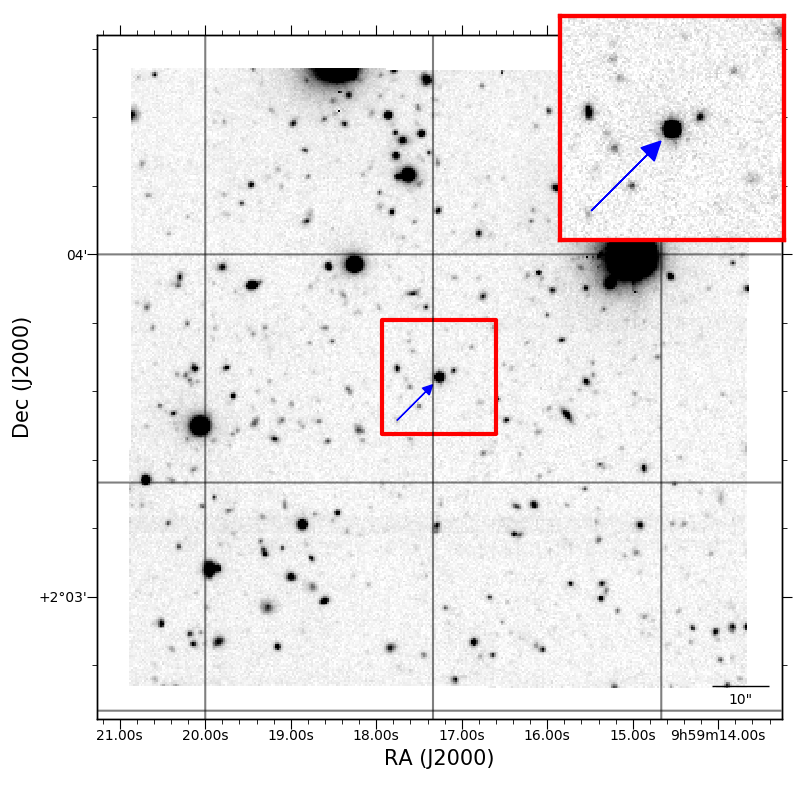
Figure 1: Finding Chart for UID 30901. Subaru $r$-band of UID 30901 taken on March, 2014.

2.1 NIR photometry

We present the time-domain $YJHK_{s}$ photometry obtained as part of the UltraVISTA survey, carried out between the 14th of December 2009 and the 29th of June 2016. UltraVISTA used VIRCAM (Dalton et al., 2006), a wide-field NIR camera mounted on the Cassegrain focus of the 4.1 m VISTA telescope (Emerson et al., 2006; Emerson & Sutherland, 2010) at Paranal Observatory. VIRCAM consists of 16 $2048\times 2048$ Raytheon VIRGO HgCdTe arrays with a mean pixel scale of 0$\aas@@fstack{\prime\prime}$34 pixel^-1. Even though the UltraVISTA survey was aimed to explore distant galaxies, their high cadence, the multi-wavelength coverage, the depth of the images ($\sim 23$ mag) and the extension of the survey make it optimal for the search for transients.

We worked with processed images, which correspond to image stacks of OB blocks of typical total exposure times of 0.5 hr or 1 hr. The processed images contain good astrometric information in their headers, so no further astrometric refinement was required. At the location of UID 30901, there is no significant host galaxy emission. However, to discover transients and remove their host galaxies a generic template subtraction strategy was applied to UltraVISTA data. The subtraction templates were constructed from images obtained in 2009 and 2010, several years before the SN explosion in the case of UID 30901. To perform the alignment between the template image and the images to be subtracted we used swarp (Bertin et al., 2002), and hotpants to do the image subtraction. hotpants uses an algorithm from Alard (2000) for the creation and application of a spatially varying convolution kernel.

Photometry was performed using a custom PSF fitting code calibrated against an UltraVISTA catalog of stars in the AB system. The UltraVISTA $YJHK_{s}$ photometry is presented in Figure 2 and summarised in Table 12 in the Appendix.

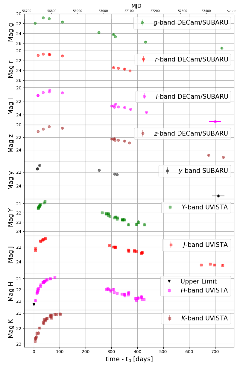
Figure 2: Optical and NIR photometry of the UID 30901

2.2 Optical photometry

In addition to the UltraVISTA NIR photometry, we present optical photometry computed from archival images obtained with the DECam instrument (Flaugher et al., 2015) mounted on the Blanco 4-m telescope, and with the HSC (Aihara et al., 2019) mounted on the 8.2 m Subaru telescope. The DECam images were downloaded using the archival online tool from the NOIRLab Database. Deep HSC $grizy$ images were downloaded from the HSC online interface , comprising images from 2014 until 2017. From these images we obtained 27 $griz$ and 25 $grizy$ individual measurements for DECam and HSC, respectively.

The $grizy$ PSF photometry was measured relative to a series of seven isolated stars close to the SN. The $griz$-band photometry of the stars was obtained from the Sloan Digital Sky Survey (Albareti et al., 2017) database, while the $y$-band photometry was downloaded using HSC online tools. The optical photometry of the SN is summarised in Table 14 of the Appendix and presented in Figure 2. The photometry of the field stars is presented in Table 15 of the Appendix.

3 Analysis

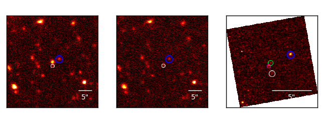
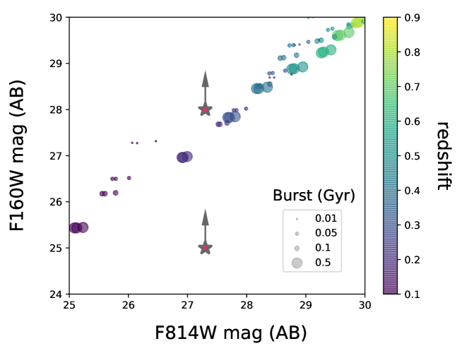
Figure 3: Finding charts for UID 30901, its host galaxy and possible galaxy companions. North is up and East is left. Left: SUBARU g-band with UID 30901 in the center. Middle: SUBARU g-band after last detection of the SN. Right: F814W image from HST WFC where the host is detected. White and blue circles mark the position of companion galaxies A and B, respectively. The green circle marks the most likely host which corresponds to the position of UID 30901 while the magenta circle presents a single detection of a non reported SN from 2004. Bottom: Synthetic F814W and F160W magnitudes obtained for the host galaxy using parameters from Perley et al. (2016). Colours represent the redshift of the galaxy and the size of the circles represent the duration of the burst. The photometry of the host is also included with two upper limits shown for the F160W filter (see text for details).

In this Section, we analyse the data of UID 30901. This includes determining the properties of the host galaxy, measuring the explosion date, characterising the light curves, deriving blackbody parameters during the early evolution and the fitting of models to the full light curves to determine the most likely power engine.

3.1 Host Galaxy

SLSNe have been found generally in low-mass faint galaxies (Schulze et al., 2018), which makes their hosts increasingly difficult to detect with increasing redshifts. An HST WFC image obtained on April 8th, 2004 using the F814W filter reveals a very faint object at the exact position of UID 30901, which we identify as its host (see Figure 3) and another point-like source that is likely to correspond to another transient, possibly another SN exploding in the same host for which no further observations are available. Photometry gives a magnitude of $27.5\pm 0.3$ for the host and $26.9\pm 0.1$ for the unidentified SN. HST NICMOS observations of the same region of the sky taken on September 9th, 2009 using the F160W filter, however, fail to show any detection. Upper limits of $\sim 28$ and $\sim 25$ magnitudes were obtained for the host assuming a point-like and galaxy-like shape, respectively. The galaxy used to model the extended shape is, however, clearly more extended than the actual host, as can be seen in the F814W image (its identification is given below), and therefore we estimate that a more realistic upper limit is found somewhere between these two extreme values.

A recent study by Ørum et al. (2020) reveals that about 50% of dwarf galaxies hosting SLSNe are found in crowded regions, independent of the redshift of the SN. Since we do not know the redshift of the host associated to UID 30901, we searched other extended extra-galactic sources with a projected distance close to the SN site as these could be companions of the host of UID 30901.

COSMOS2015 (Laigle et al., 2016) is a photometric redshift catalogue including deep imaging from UltraVISTA DR2 (McCracken et al., 2012), SUBARU (Suprime-Cam and Hyper Suprime-Cam) and Spitzer (SPLASH catalog, see Steinhardt et al., 2014, Section 2) among other telescope-instrument combinations from previous surveys of the $\sim$ 2 degrees² COSMOS area in the sky. We inspected the COSMOS2015 deep catalogs in search for galaxies close to our object. We found two candidates in a 5$\aas@@fstack{\prime\prime}$0 radius circle around the object position. These galaxies, designated as A and B, at distances of 1$\aas@@fstack{\prime\prime}$5 South and 2$\aas@@fstack{\prime\prime}$5 North-West respectively from the SN location, are shown in Figure 3. Galaxy B, a clearly bright and extended source, is detected in the NICMOS F160W image and was used as a model to determine the upper limit of the host.

The photometry of galaxy B was already measured in previous COSMOS surveys: Capak et al. (2007); Ilbert et al. (2009), yielding a photometric redshift estimate of $z=0.53$. The photometric redshift of A is poorly constrained, having a median of $z=1.61$ and a peak of probability at $z=0.37$. COSMOS2015 reports the median as the photo-z result calculating a 68% confidence interval around it. Similarly, other fitted quantities such as stellar mass, star formation rate and age are given for both values, but the error bars are only reported for those coming from the median of the $z$ probability distribution.

In Section 3.4 we show that it is unlikely for UID 30901 to have a redshift larger than one. In such a case, we would be observing the near and far UV rest-frame light curves in the $g$ and $r$ filters respectively, but the radiation measured in those bands does not resemble the expected abrupt decrease at those wavelengths for this (or any) kind of SN. Similarly, from our blackbody fitting, we find that photospheric temperatures consistent with such a redshift would be large (between 20,000 and 30,000 K) during the first couple of weeks of observations. Besides, $z=1.0$ would imply an absolute magnitude for UID 30901 $M_{\rm abs}\lesssim-23.5$ mag, while no SN event of such luminosity has been ever observed. Hence, if galaxy A is found at the same redshift as the host of UID 30901, we can reject a $z=1.61$ value. Instead, we adopt the peak redshift of $z=0.37$ as representative.

Having tentative redshifts for the SLSN of 0.53 and 0.37, and an upper limit of $z<1$, we tested whether the F814W magnitude and the F160W upper limits are consistent with these $z$ values. Using the Flexible Stellar Population Synthesis code (Conroy et al., 2009; Conroy & Gunn, 2010), we obtained synthetic magnitudes for the host of UID 30901 for a redshift range of $0.1\leq z\leq 0.9$ after assuming the usual parameters for SLSN hosts as described by Perley et al. (2016). That is, an old population that contributes to a stellar mass in the $10^{6-8}$ M_⊙ range, a recent burst with constant star formation rate (SFR) of $0.03-3$ M_⊙yr^-1, ages for the burst of $10-500$ Myr, and a modest amount of extinction of A_V = 0.0, 0.1 and 0.5 magnitudes.

We find that given the faint magnitudes of our host, only small host masses ($10^{6}$ M_⊙), low SFRs ($0.03$ _⊙yr^-1) and redshifts below 0.5 are in agreement with our data. The burst duration is the variable that introduces most of the vertical scatter to the trend seen in Figure 3, followed by extinction. We also find that the point-like upper limit for the F160W filter is found in agreement with the synthetic data, implying that the host of UID 30901 could be a very compact source.

Our previous results agree well with the redshifts found for galaxies A and B, which have projected distances of 7 and 15 kpc to the SLSN host, respectively, for assumed redshifts of 0.37 and 0.53. For the remainder of this work, we will adopt these redshifts as representative candidate-$z$ values for the host of our SLSN. Coordinates and photometry of the host and possible companion galaxies are detailed in Table 1.

Host Galaxy
Parameters
RA	149.821917
DEC	2.060639
mag F814W	27.30(17)
mag F160W	…….
Companion Galaxies
Parameters	A	B
RA	149.821884	149.821243
DEC	2.06029	2.060975
Ang. Dist.	1.45"	2.54"
mag $g$	26.98(28)	25.70(10)
mag $r$		24.90(06)
mag $i$	26.96(18)	24.56(04)
mag $z$	26.20(20)	24.41(07)
mag $y$		24.24(13)
UltraVISTA
mag $Y$	26.09(12)	24.27(03)
mag $J$	25.45(10)	24.29(05)
mag $H$	25.59(18)	24.57(10)
mag $K$	25.41(15)	24.34(08)
SuprimeCam
mag $B$	27.65(23)	26.31(10)
mag $V$	27.39(30)	25.59(09)
mag $r$	26.93(19)	24.98(05)
mag $i$	27.19(33)	24.67(05)
mag $z$	26.42(18)	24.44(04)
COSMOS2015${\dagger}$
ID${\dagger}$	499317	500106
photo-z median	1.61${}_{-0.52}^{+0.69}$	0.52(04)
photo-z best-fit	0.37	0.53
Age [years]	$5\times 10^{7}$	$9.05\times 10^{8}$
SFR [log10]	0.59	-1.29
sSFR [log10]	-7.34	-9.57
Proj. Dist [Kpc]	7.4	15.4
Stellar Mass [log10 $M_{\odot}$]	7.93	8.28

• ${\dagger}$: Laigle et al. (2016). Only best-fit derived quantities are considered (see text).

Table 1: Properties of the host and possible companion galaxies. Top: we present coordinates and photometry measured from the single image of HST. Middle: we present coordinates, angular distance to the SN position, and photometry we measured from SUBARU Hyper SuprimeCam optical images taken when the SN was not present. Bottom: COSMOS2015 photometry and resulting parameters from SED fittings. The photometry includes deep imaging from UltraVISTA and SUBARU SuprimeCam among other sources.

3.2 Explosion date: Power Law and Linear Fits

3.2.1 Rise Time Fits

A power law model for the flux $F\propto(t-t_{0})^{\alpha}$ has been used often to characterise the early part of a diverse number of transients. In our case, the power law provides a good fit to the rising part of the NIR data, and therefore can be used to estimate the explosion date.

To fit a power law we first transformed our $YJHK_{s}$-band photometry to flux units. Next, we fit the early $YJHK_{s}$-band light curves simultaneously with a six parameter power law model: four constants (one for each band) the time of explosion ($t_{0}$) and the power law exponent ($\alpha$). We also fit a linear model to the flux, due to the linear behaviour seen in the middle section of the rise time. In both cases we used a MCMC code based on the emcee python package (Foreman-Mackey et al., 2013). The results for both fits are summarised in Table 2 and a plot of the fit is shown in Figure 4.

Our power law model places the explosion date $\sim$ 6 days before the first detection, while the linear fit places the explosion $\sim$ 15 days earlier. Both estimates are in the observer frame. We did not include the optical photometry in the fitting as it is not well sampled in the early phase of the light curves. In what follows we will compare these extrapolations with the other observational constraints.

3.2.2 Explosion Date

UID 30901 was first detected on March 17th, 2014 at 03:10 UT time in the $H$ band by UltraVISTA using VIRCAM on the VISTA telescope at Paranal and 10 minutes later was detected by DECam in $g$ band mounted on Blanco telescope at CTIO. A deep VISTA $H$-band image taken on March 12th at 03:21 UT time shows no signal of the SN. We added artificial stars to the non-detection image of diverse brightness and tried to detect them using the DAOFIND algorithm (Stetson, 1987), looking for the brightness value that reaches a 50% of detection rate. With this process, we estimated a limiting magnitude of 23.3 in the deep $H$-band image (see Figure 4). This corresponds to less than 10% of the $H$-band flux at peak and is $\sim 0.1$ mag below the linear fit to the early part of the light curve.

Based on our fits of the early data points and the limiting magnitude obtained five days before the first detection, we estimate an explosion epoch of March 10th, 2014.

Table 2: Early part of the light curves.

Linear Fit
$t_{0}$ [MJD]	56718.5(6)
Power Law
$t_{0}$ [MJD]	56727.5(5)
$\alpha$	0.72(03)
Last Non-Detection
$t_{ND}$ [MJD]	56728.14
First Detection
$t_{1}$ [MJD]	56733.13

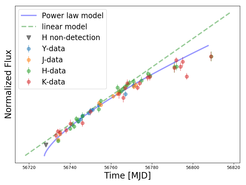
Figure 4: Linear and Power Law fit of the early part of the light curve.

3.3 Comparison with other supernovae

To get further insights into the nature of UID 30901, we compare its $r$-band absolute magnitude light curve with low-z stripped-envelope SNe from the Carnegie Supernova Project I (Hamuy et al., 2006; Stritzinger et al., 2018a), with SLSNe from the Pan-STARRS1 Medium Deep Survey (Lunnan et al., 2018) and the Dark Energy Survey (Angus et al., 2019). We also compare the UID 30901 spectral energy distribution (SED) with the spectra of superluminous SNe at two representative epochs separated by more than a hundred days: near maximum light and at a later phase.

3.3.1 Light curve comparison

Looking carefully at the light curve evolution of SN UID 30901 (see Figure 2) we can readily dismiss the hypothesis that it could correspond to a SN Ia or to a normal SN II. This is based on the fact that SNe Ia peak earlier in the NIR than in the optical (see Folatelli et al., 2010), they have narrower light curves than UID 30901, with typical rise times of about 15 to 20 days in the rest-frame (see e.g., Firth et al., 2015), and display distinctive double peaked light curves in the NIR. None of these characteristics are observed in the light curves of UID 30901. Similarly, normal type II SNe display a rise time to maximum in the optical of less than 30 days, and they often display a ‘plateau’ phase followed by a rapid decline once the hydrogen-rich ejecta has recombined to finally settle in a radioactive tail at about 80 to 150 days after the explosion (see e.g., Anderson et al., 2014, for more details). Again, these characteristics are not observed in the UID 30901 light curves (see Figure 2).

The comparison with Stripped Envelope SNe can be seen more clearly in Figure 5, where we plot the $r$-band light curve of UID 30901 and the optical photometry of stripped-envelope SNe from the CSP-I sample (Stritzinger et al., 2018a; Taddia et al., 2018). The redshift value required to make the $r$-band maximum brightness of UID 30901 consistent with the mean $r$-band absolute magnitude of the Type Ic CSP-I subsample ($M_{r}=-17.7\pm 0.2$ mag) is $z\approx 0.1$. Similarly, $z\approx 0.25$ makes the $r$-band maximum brightness of UID 30901 consistent with a bright SN Ic-BL ($M_{r}\approx-19.9$ mag). All the relevant parameters such as the time of $r$-band maximum, redshift, luminosity distance, and Galactic and host galaxy extinction values for the CSP-I SNe were adopted following Taddia et al. (2018). The host galaxy reddening reported by Taddia et al. (2018) was computed following the methodology presented by Stritzinger et al. (2018b). As can be seen, the light curve of UID 30901 is significantly broader than any of these SN types, rejecting the possibility of a normal luminosity stripped-envelope SN origin for UID 30901, and suggesting a longer diffusion timescale and therefore a more massive SN ejecta for this object.

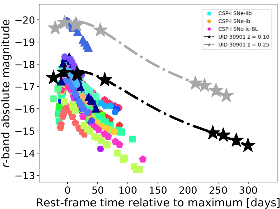
Figure 5: Comparison between the $r$-band absolute magnitude of UID 30901 and the stripped-envelope SNe from CSP-I (Stritzinger et al., 2018a; Taddia et al., 2018) after assuming redshifts of $z=0.10$ (black stars) and $z=0.25$ (grey stars), to make its luminosity at maximum consistent with a normal SN Ic and a relatively bright Ic-BL, respectively. In the figure SNe type IIb are shown as squares, type Ib as pentagons, type Ic as circles and type Ic-BL as triangles. As can be seen the light curve of UID 30901 is broader than any of these SN types.

Next, we compare the light curve of UID 30901 with other SLSNe to confirm its superluminous nature. In Figure 6, the $r$-band absolute magnitude light curve of UID 30901 is presented when assuming redshifts of $z=0.37$ and $z=0.53$ (see Section 3.1). These are compared with SLSNe from PS1 (Lunnan et al., 2018) and DES (Angus et al., 2019) for the redshift range $0.25\leq z\leq 0.65$ to avoid the need of k-corrections, and the Type II superluminous SN 2006gy (Smith et al., 2007). The time of maximum light for the PS1 and DES SNe was computed using Gaussian process interpolation as described in Cartier et al. (2021), and the light curves were corrected by Galactic reddening ($E(B-V)$) as reported by Schlafly & Finkbeiner (2011) using the Cardelli et al. (1989) extinction law. For SN 2006gy the $A_{R}$ values reported by Smith et al. (2007) were used for the reddening correction, this is $A_{R}=0.43$ and $A_{R}=1.25$ for our galaxy and the SN host galaxy, respectively. No k-corrections were applied to the light curves as we expect this correction to be of the order of a few tenths of magnitude for the highest redshift objects, which is small compared to the dispersion observed in the maximum luminosity and with the light curve shape diversity displayed by SLSNe (see De Cia et al., 2018; Lunnan et al., 2018; Angus et al., 2019; Cartier et al., 2021).

Looking at Figure 6 we find that the shapes of luminous ($M_{r}<-20$ mag) SLSNe are similar to UID 30901, thus confirming its superluminous nature. UID 30901 is among the objects with the broadest light curves, regardless of the redshift assumed for this SN. Aside from a small group of fainter SLSNe with maximum brightness $M_{r}\gtrsim-20$ mag, showing light curves shapes that could be consistent with a bright SN Ic-BL, all SLSNe with broad light curves such as UID 30901 have maximum luminosities $M_{r}<-20$ mag. Unless UID 30901 is a very peculiar object with a very broad light curve and a moderate luminosity, we can safely assume that UID 30901 has a maximum absolute magnitude $M_{r}<-20$ mag, implying that its redshift must be $z>0.25$.

A review of the literature reveals that the brightest SLSNe reported have absolute magnitudes in the range of $-22.0$ mag $\lessapprox M_{\mathrm{abs}}\lessapprox-22.5$ mag (Smith et al., 2007; Vreeswijk et al., 2014; Smith et al., 2016; De Cia et al., 2018; Smith et al., 2018; Lunnan et al., 2018; Cartier et al., 2021; Yin et al., 2021). Therefore assuming that UID 30901 reached one of the brightest maximum luminosities reported for a SLSNe ($M_{r}\approx-22.5$), we can place an approximate redshift upper limit of $z\lesssim 0.7$ for this SN.

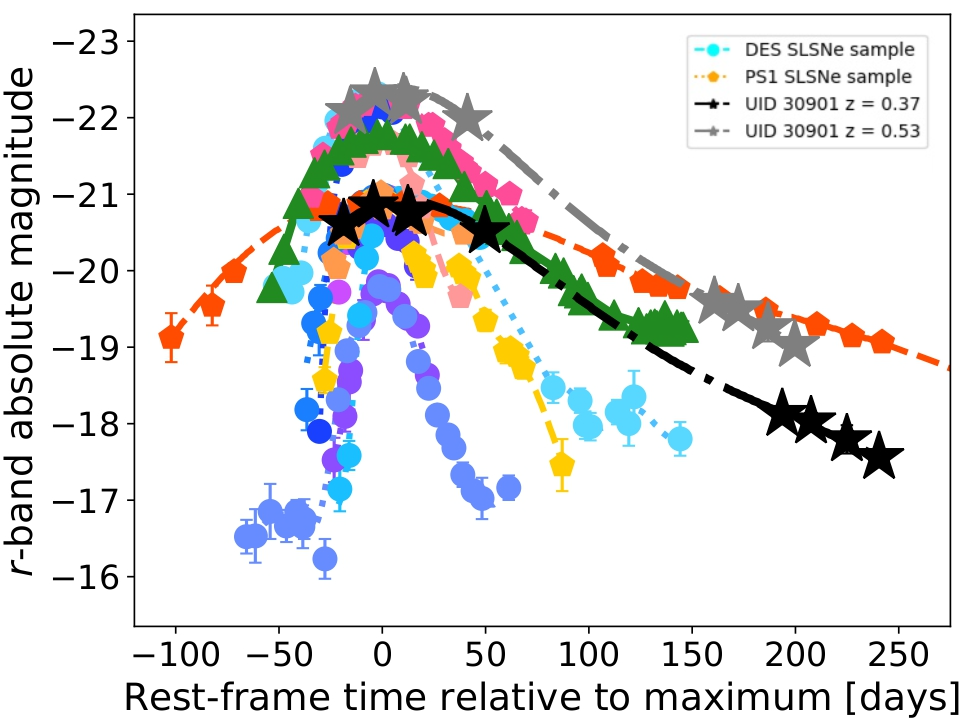
Figure 6: Comparison between the $r$-band absolute magnitude of UID 30901 and SLSNe from PS1 (Lunnan et al., 2018), DES (Angus et al., 2019) and SN 2006gy (Smith et al., 2007). For PS1 and DES SLSNe we show the Gaussian process $r$-band light curve interpolations presented in Cartier et al. (2021). PS1 SLSNe are shown as pentagons and their light curve interpolations with dotted lines, DES SLSNe are shown as circles and their light curve interpolations using dashed lines, SN 2006gy is shown as green triangles and the host galaxy distance and reddening are from (Smith et al., 2007). We show SN UID 30901 assuming at z=0.37 (black stars) and at z=0.53 (grey stars)

.

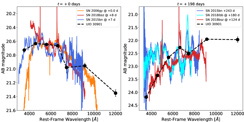
Figure 7: SED comparison between UID 30901 and other SLSNe assuming z=0.37. In the left-panel the SED of UID 30901, the spectra of SLSNe-I SN 2015bn (Nicholl et al., 2016a) and SN 2018bsz (Anderson et al., 2018), and the spectrum of the SLSN-II SN 2006gy (Smith et al., 2007) are compared within days of maximum light. In the right-panel the late phase SED of UID 30901 (+198 days) and the late time spectra of SLSNe SN 2015bn (Nicholl et al., 2016a), SN 2018ibb, SN 2018bsz are compared. It can be seen that after maximum light SN 2018bsz starts to interact with a dense CSM displaying a strong H$\alpha$ emission line and evidence for dust condensation (see Chen et al., 2021). The late spectra of SN 2018bsz and SN 2018ibb were obtained with the Goodman spectrograph mounted at SOAR telescope, and are presented here for comparison but will be published elsewhere.

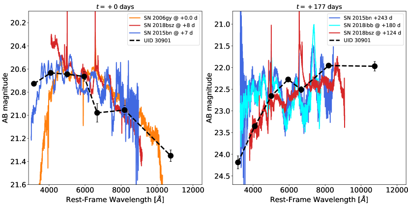
Figure 8: Same as Figure 7, but in this case assuming z=0.53.

3.3.2 Spectral energy distribution

The comparison of the light curve of UID 30901 with the diversity of SN types has shown that this object displays a broad light curve, which is only consistent with a SLSN. From this, we have placed constraints on the redshift of this object to be in the range of $0.25<z\lesssim 0.7$. This redshift range is in agreement with the photometric redshifts of the potential host galaxies discussed in Section 3.1. In the following, we will compare the $grizYJH$ SED of UID 30901, at $\mathrm{MJD}=56764$ (at about maximum bolometric luminosity) and at $\mathrm{MJD}=57035$ (+271 d after maximum in the observer frame), with other SLSNs using the redshift values for the potential host galaxies from Section 3.1.

In the left panel of Figure 7 we compare the SED of UID 30901 after assuming $z=0.37$ with the spectra of SLSNe SN 2015bn (Nicholl et al., 2016a), SN 2018bsz (Anderson et al., 2018) and SN 2006gy near the time of maximum luminosity. At this phase the SED of UID 30901 is well reproduced by a blackbody (see Section 3.5) and it is also in very good agreement with the spectrum of SN 2015bn, while the near maximum spectra of SN 2018bsz (Anderson et al., 2018) appears too blue, and the spectra of SN 2006gy seems too red, even after correcting them by Galactic and host galaxy reddening. Assuming $z\simeq 0.37$, the $Y$-band flux drop in UID 30901 coincides with the strong O i $\lambda 7774$ absorption line in the spectrum of SN 2015bn. In Figure 8 a similar comparison is presented but assuming $z=0.53$, where the SED of UID 30901 is again similar to SN 2015bn, but at this redshift the drop in the $Y$ band no longer coincides with the O i $\lambda 7774$ absorption line. The overall spectrum of SN 2015bn coincides better with UID 30901 assuming $z=0.37$.

In the right panel of Figure 7 the SED of UID 30901 is compared with the spectra of SN 2015bn (Nicholl et al., 2016b), SN 2018bsz and SN 2018ibb. The spectra of SN 2018bsz and SN 2018ibb were obtained with the Goodman spectrograph mounted at the SOAR telescope, and are presented here for comparison but will be published elsewhere. Assuming $z=0.37$, the SED of UID 30901 shown in the right panel of Figure 7 corresponding to $+200$ d in the rest frame, and it has evolved dramatically becoming very red below 6500 Å when compared to the SED at maximum light. The spectra of SN 2015bn or SN 2018ibb, which are representative of a “normal" SLSN-I at a late phase no longer provide the best comparison to the SED of UID 30901 at this phase. These two SNe are bluer by nearly one mag at 4000 Å compared with UID 30901. On the other hand, the spectrum of SN 2018bsz at +124  days provides a good comparison to the SED of UID 30901. SN 2018bsz was classified as the closest SLSN I, at a redshift of $z=0.0267$ (see Anderson et al., 2018). It showed some unusual features including a long plateau before maximum light. After maximum, it started to show a strong and broad H$\alpha$ emission, evidence of ejecta-CSM interaction, and also indications of dust formation (Yan et al., 2017). In the right panel of Figure 7, the $z$-band of UID 30901 coincides and provides a good match to the H$\alpha$ emission in SN 2018bsz. Assuming $z=0.53$ (right panel of Figure 8), SN 2018bsz also provides the best comparison to the UID 30901 SED, but the agreement is not as good as assuming $z=0.37$.

3.4 Characterising the light curves

To characterise the light curves of UID 30901 we used a simple polynomial fitting to interpolate the photometry. Three phases were distinguished in our light curves. The early phase comprises the rise to maximum, the time of the maximum, and in some optical bands the beginning of a decline from the peak brightness. During the second phase, between +200 and +380 days post peak, the SN shows a nearly linear decline, as we will show below. Finally, the last phase comprises observations from +594 days to our last detection at +685 days observer frame, where the SN seems to decline at a slower rate compared to the previous phase.

3.4.1 Early Phase

To characterise the rise to the peak and the decline of the light curves of UID 30901, we fit a low order polynomial. These fits provide an estimated epoch of the maximum and the peak magnitude in the optical bands. The NIR light curves do not have any photometric points beyond maximum and hence no early decline is observed. However, in the $H$ and $K_{s}$ bands the light curves seem to reach close to the peak. Hence, for the NIR bands we can place lower limits in MJD and upper limits in magnitudes for the maximum. We report our results in Table 3 and in Figure 9.

As can be seen in Figure 9 our multi-wavelength coverage suggests a relation between the epoch of peak brightness and the observed effective wavelength, where longer effective wavelengths peak later. This relation seems to extend to the NIR bands, where the NIR bands reach their peak brightness after the optical bands. We note that this behaviour of reaching maximum brightness later at longer effective wavelengths is similar to the one reported in well-observed SNe Ic and Ic-BL (e.g., Hunter et al., 2009; Pignata et al., 2011; Taddia et al., 2018) and as noted in the previous section is different from the behaviour observed in SNe Ia, where the NIR bands ($iYJHK_{s}$) reach their peak brightness between 3 to 5 days before the $B$-band maximum (which is similar to the time of the $g$-band maximum; see Folatelli et al., 2010).

Table 3: Peak light curve information for UID 30901.

Filter	MJD	Observed	z=0.37	z=0.53
	(days)	(mag)	(mag)	(mag)
$g$	$56766$($07$)	$20.78$($05$)	-20.64	-21.63
$r$	$56770$($10$)	$20.67$($04$)	-20.75	-21.66
$i$	$56800$($11$)	$20.36$($13$)	-21.06	-22.05
$z$	$56807$($07$)	$20.34$($07$)	-21.08	-22.07
$Y$	$>56771.1$	$<20.77$	$<-20.65$	$<-21.64$
$J$	$>56772.1$	$<20.86$	$<-20.56$	$<-21.55$
$H$	$\geq 56809.0$	$\leq 20.89$	$\leq-20.53$	$\leq-21.52$
$K_{s}$	$\geq 56829.0$	$\leq 21.05$	$\leq-20.37$	$\leq-21.36$

• Numbers in parenthesis correspond to 1-$\sigma$ statistical uncertainties. The given peak absolute magnitudes correspond just to apparent magnitude minus the distance modulus in a $\Lambda CDM$ Universe with $\Omega_{M}=0.3$, $\Omega_{\Lambda}=0.7$ and Hubble-Lemaitre parameter $h=0.7$.

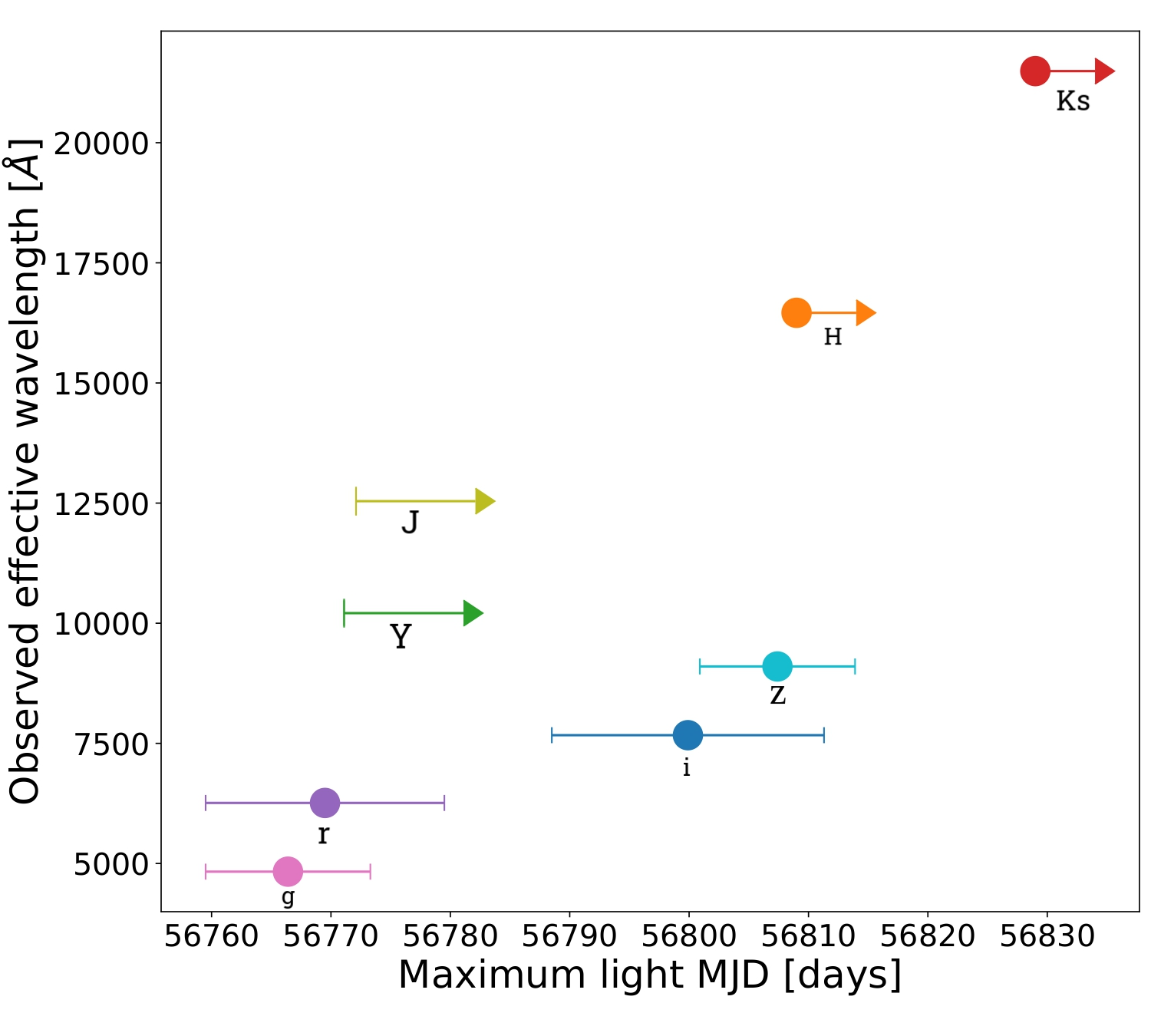
Figure 9: Epoch of maximum light for different bandpasses. For the NIR bands we present a lower limit of the time of maximum light, observations of $H$ (in orange) and $K_{s}$ (in red) bands seem to be very close to peak. Our estimates for the epoch maximum light suggests an increase of the time of maximum with wavelength.

3.4.2 Linear Decline Phase

From November 2014 to May 2015 the light curves of UID 30901 display a post maximum linear decline, hence we fit a linear model to measure the decline rate, interpolate, and in some cases extrapolate the light curves over this period. To assess the goodness-of-fit of the linear model we computed the reduced chi-squared ($\chi^{2}_{\nu}$) and the root mean squared ($\mathrm{\it rms}$).

We summarise the decline rates of the $grizyYJH$ bands, the $\chi^{2}_{\nu}$ and the $\mathrm{\it rms}$ of the fits in Table 4, and we present the linear model residuals in Figure 10. Although a linear fit may be considered a too simplistic model, the residuals, the $\chi^{2}_{\nu}$, and the $\mathrm{\it rms}$ indicate that a linear model is an adequate approximation to the SN luminosity decline over this phase (see Figure 10).

Table 4: Linear decline rate information for UID 30901.

Filter	Observed decline rate	Decline rate at $z=0.37$	Decline rate at $z=0.53$	$\chi^{2}_{\nu}$	$\mathrm{\it rms}$	$n_{\mathrm{obs}}$
	(mag/100 days)	(mag/100 days)	(mag/100 days)		(mag)
$g$	$1.09$($0.06$)	$1.49$($0.09$)	$1.67$($0.09$)	$4.26$	$0.087$	$4$
$r$	$0.89$($0.15$)	$1.22$($0.21$)	$1.37$($0.23$)	$0.16$	$0.022$	$4$
$i$	$0.72$($0.07$)	$0.98$($0.09$)	$1.10$($0.10$)	$3.76$	$0.054$	$8$
$z$	$0.89$($0.11$)	$1.17$($0.15$)	$1.31$($0.17$)	$1.52$	$0.032$	$7$
$y$	$0.90$($0.05$)	$1.24$($0.06$)	$1.38$($0.07$)	$0.76$	$0.011$	$3$
$Y$	$0.97$($0.04$)	$1.33$($0.06$)	$1.48$($0.06$)	$1.66$	$0.031$	$21$
$J$	$0.72$($0.04$)	$0.98$($0.06$)	$1.10$($0.06$)	$0.70$	$0.019$	$16$
$H$	$0.63$($0.04$)	$0.87$($0.06$)	$0.97$($0.06$)	$1.40$	$0.026$	$23$

• Numbers in parenthesis correspond to 1-$\sigma$ statistical uncertainties.

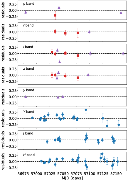
Figure 10: Residuals from the linear fits to the light curves of UID 30901 from November 2014 to May 2015. We present the DECam/Blanco ($griz$) residuals as red squares, the ($grizy$) HSC/SUBARU residuals as purple triangles, and the VISTA ($YJH$) residuals as blue circles. In the top-left of each panel we indicate the corresponding band.

Recently De Cia et al. (2018) analysed a sample of 26 spectroscopically confirmed hydrogen-poor SLSNe from the (i)PTF survey. They measured the rest-frame $g$-band decline rate after 60 days from the $g$-band maximum and found a range of decline rates from $\sim 0.25$ to $\sim 2.25$ mag/100 days for their sample, with a mean of $1.3\pm 0.5$ mag/100 days. If UID 30901 is at $z\simeq 0.37$, the $r$-band would be similar to the rest-frame $g$-band, and the measured $r$-band decline rate would be $1.22\pm 0.21$ mag/100 days agreeing very well with the mean decline rate of the SLSN sample analysed by De Cia et al. (2018). If UID 30901 is at $z\simeq 0.53$, the rest-frame $g$-band would cover part of the $r$ and $i$ bands, with the rest-frame effective wavelength found in the $i$-band. The decline rate values are found to be $1.37\pm 0.23$ and $1.10\pm 0.10$ for the $r$ and $i$ bands, respectively, which compare well with the rest-frame $g$-band decline rates reported by De Cia et al. (2018).

3.4.3 Final Year Characterisation and Flattening at Late Epochs

We have sparse observations from December 2015 to March 2016 in several bands. Some of them are the results of combining several frames over about a month to obtain a SN detection at very faint magnitudes, as is the case of the $iyJ$-bands.

Table 5: Linear decline rate information for the final year of UID 30901.

Band	Observed	$z=0.37$	$z=0.53$	Brightness at
	(mag/100 days)	(mag/100 days)	(mag/100 days)	MJD=57428.0
				(mag)
$z$	$0.5$($0.3$)	$0.7$($0.4$)	$0.8$($0.4$)	$25.0$($0.1$)
$J$	$0.1$($0.2$)	$0.2$($0.3$)	$0.2$($0.3$)	$24.4$($0.1$)

• Numbers in parenthesis correspond to 1-$\sigma$ statistical uncertainties. Two and four epochs were used for the $z$ and $J$ bands, respectively

Table 6: Difference between observed magnitudes in the last observing season and a linear fit extended from the linear decay phase.

Band	MJD	Residuals	$\sigma_{phot}$	$\sigma_{fit}$	$\sigma_{magtot}$	$\sigma$
		(mag)	(mag)	(mag)	(mag)	(mag)
$g$	57454.329	-2.0	0.18	0.26	0.31	6.6
$i$	57428.0	-0.5	0.19	0.25	0.31	1.7
$z$	57402.669	-0.6	0.12	0.39	0.41	1.5
$z$	57459.474	-0.8	0.12	0.45	0.47	1.7
$y$	57440.0	-0.4	0.21	0.19	0.28	1.5
$J$	57374.099	-0.0	0.13	0.12	0.18	0.04
$J$	57408.758	-0.4	0.09	0.13	0.16	2.3
$J$	57425.337	-0.4	0.16	0.16	0.22	1.6
$J$	57457.943	-0.5	0.14	0.18	0.23	2.3

Table 7: Decline rate at second and final year of observing season of UID 30901

Band	Linear phase	Last year	$\Delta$	$\sigma$
	(mag/100 days)	(mag/100 days)	(mag)	(mag)
z	0.9(0.1)	0.5(0.3)	0.4(0.3)	1.3
J	0.72(0.04)	0.1(0.2)	0.6(0.2)	2.7

During the linear decline phase, the $z$-band shows a decline rate of 0.89 $\pm$ 0.11 mag/100 days after which it drops to 0.53 $\pm$ 0.26 mag/100 days in the final year, as determined from two points seen in the late light curve. The difference in the decline of the $J$-band is even higher. While in the linear phase the $J$-band declines at 0.72 $\pm$ 0.04 mag/100 days, in the final year it drops to 0.13 $\pm$ 0.22 mag/100 days. These changes correspond to a decrease in the decline rates of 0.36 $\pm$ 0.28 mag/100 days and 0.59 $\pm$ 0.22 mag/100 days, at a 1.3 and 2.7 sigma level in the $z$ and $J$ bands, respectively. In Section 3.6.2 we show that the late decline rates are not consistent with the ⁵⁶Ni radioactive decay. We summarise our results in Table 5.

Table 8: Individual slope measured for individual $gizyJ$ bands

Band	$\alpha$	$n_{obs}$
g	-2.8	5
i	-2.7	7
z	-3.2	8
Y	-3.3	22
J	-3.0	17

A different approach to assess the potential flattening in the light curves is the difference between the photometric observations in the final year and the extrapolation of the linear model fitted to the second observing season. These differences yield consistently negative residuals summarised in Table 6 which means that the SN remains consistently brighter in all bands and at all epochs in the final year when compared with the brightness expected from the linear extrapolation. It is important to notice that: 1) the linear fits are based on several observations, therefore the parameters and their errors are considered robust, and 2) the majority of the core collapse and thermonuclear SNe, powered by radioactive decay are well modelled by a linear decline rate from about a hundred days to several hundred days after the explosion.

The fact that all bands ($gizy$ and $J$) at all late epochs exhibit brighter magnitudes than the ones predicted by the linear extrapolation implies that this is not an artefact produced by random errors in the photometry. Additionally, the $z$ and $J$ bands which have more than one epoch in the last observing season show a decrease in their residuals (increase in absolute value) with time. The residual in $z$ decreases from -0.6 $\pm$ 0.4 mag to -0.8 $\pm$ 0.5 mag over 57 days in the observed frame. Similarly, the $J$ band residuals decrease from -0.01 $\pm$ 0.18 mag to -0.52 $\pm$ 0.23 mag over nearly 84 days, suggesting a pronounced flattening and deviation with time from the linear decline model. The uncertainties here correspond to the sum in quadrature of the photometric uncertainties and the linear model uncertainties, the latter being the dominant source of uncertainty.

The apparent flattening is remarkably pronounced in $g$-band, where the measured residual is -2.0 $\pm$ 0.3 mag or a 6.6 sigma deviation from the extrapolated linear decline model. There is an apparent tendency for bluer bands to have a more pronounced deviation from the linear extrapolation compared to redder filters at similar epochs. The notable deviation from the linear decline measured in $g$-band via these residuals could be, in part, explained by the large decline rate observed over the second observing season, which predicts a much faster dimming of the SN in this band compared to others.

Other SLSN light curves have also been observed to flatten at late epochs. SN 2015bn (Nicholl et al., 2018) and SN 2016inl (Blanchard et al., 2021) exhibit a flattening similar to UID 30901 and a decline rate significantly slower than the radioactive decay of ⁵⁶Ni. In order to compare the three objects we fit a power law to the last two sections of the individual $gizy$ and $J$ bands finding values that range from $L_{i}\propto t^{-2.8}$ to $L_{Y}\propto t^{-3.3}$ (see Table LABEL:tab:tail_plaw). We also measure a $L_{r}\propto t^{-4.0}$ for SN 2015bn at the same rest-frame phase assuming $z=0.37$, while Blanchard et al. (2021) report a decline of $L\propto t^{-2.8}$ in the combined $r+$F625W filters for SN 2016inl found at $z=0.31$. In summary, UID 30901 and SN 2016inl show a similar degree of flatness in their late-time evolution, while both SLSNe have shallower power-law indices than SN 2015bn.

3.5 Blackbody Model

Armed with the light curve interpolations described in Section 3.4, we now proceed to fit a blackbody model.

The high densities and temperatures that prevail in the early stages of the explosion make the blackbody a good fit to the data and useful to estimate basic physical parameters, such as the bolometric temperature ($T_{bb}$) and radius ($R_{bb}$) of the SN, regardless of the mechanism behind the event.

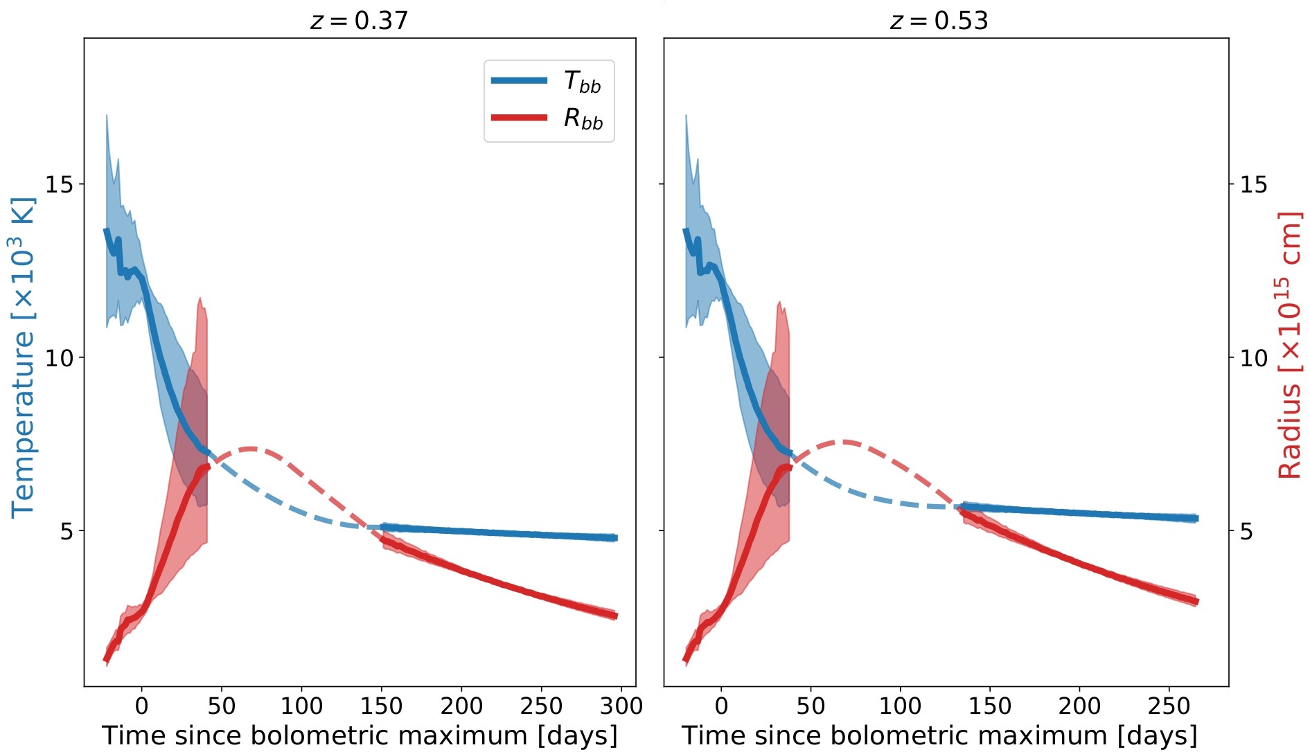
Figure 11: Blackbody temperature ($T_{bb}$; in blue) and radius ($R_{bb}$; in red) as a function of rest-phase time since bolometric maximum. We present these parameters from our blackbody fits to the interpolated photometry for the redshifts equal to $0.37$ and $0.53$. The dashed lines represent an interpolation of $T_{bb}$ and $R_{bb}$.

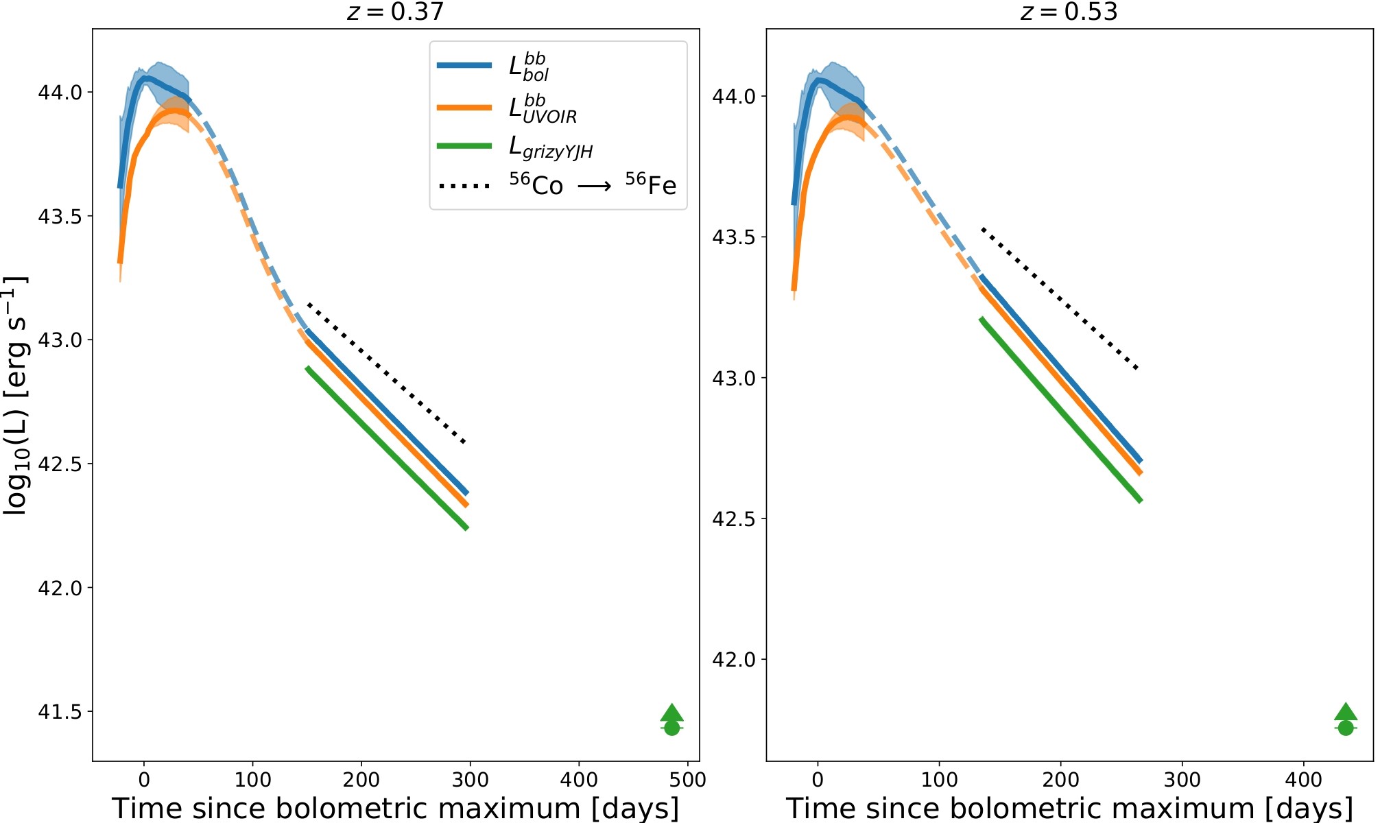
Figure 12: Bolometric luminosity ($L_{\mathrm{bol}}$; in blue), UVOIR pseudo-bolometric luminosity ($L^{bb}_{\mathrm{UVOIR}}$; in orange), and the pseudo-bolometric luminosity ($L_{\mathrm{grizyYJH}}$; in green) obtained from summing over the luminosity emitted in the observed bands, at redshifts equal to $0.37$ and $0.53$. The blue and orange dashed lines correspond to $L_{\mathrm{bol}}$ and $L^{bb}_{\mathrm{UVOIR}}$ computed using the interpolated values of $T_{bb}$ and $R_{bb}$. The black-dotted lines correspond to the ⁵⁶Co decay.

In the early phase we only interpolate observations and do not perform any extrapolations. In this phase, we always have observations in at least three bands to fit a blackbody model. Typically we have seven bands from $g$ to $K_{s}$ bands, providing an excellent leverage to get reliable blackbody parameters.

For the linear decline phase, we interpolate and extrapolate the light curves from MJD=56970.0 to MJD=57168.0, as described in Section 3.4.2. During this phase, the blackbody model does not provide a precise description of the observations. But this is expected as SLSN spectral energy distributions (SEDs) is dominated by absorption and emission lines deviating from a perfect blackbody. However, the blackbody fits provide a good approximation to the pseudo-photospheric temperature and serve to estimate the total bolometric emission.

For the late phase, we estimate a single pseudo-bolometric data point at MJD = 57428.0 computed from summing the flux over the $gizy$ and $J$ bands. To do this we used observations obtained close in time for the $giy$ bands, and linearly interpolated the $z$ and $J$ bands, since these two bands have several individual observations over this light curve phase.

To perform our blackbody fits, we assumed host galaxy redshifts of $0.37$, and $0.53$ as described in Section 3.1. In Figure 11 we present $T_{bb}$ and $R_{bb}$ and in Figure 12 we present the bolometric luminosity ($L_{\mathrm{bol}}$), the UVOIR pseudo-bolometric luminosity ($L^{bb}_{\mathrm{UVOIR}}$) computed by integrating the blackbody emission from $3000$ to $20000$ Å  in the rest-frame, and the pseudo-bolometric luminosity ($L_{\mathrm{grizyYJH}}$) obtained from summing over the luminosity emitted in the observed bands, at these redshifts.

3.5.1 UV absorption

One of the main spectral features of SLSNe is the significant absorption in the UV part of the SED at the pre-peak phase (Quimby et al., 2011). Recently Yan et al. (2018) present four UV spectra from different SLSNe showing that the emission at $\lambda<2800\$ Å is considerably lower than the blackbody model. This absorption should leave an imprint in our blackbody models. Based on this, we examine the SED of UID 30901 at MJD$\sim$56764.0 in Figure 13, only one day after maximum light when the blackbody assumption is highly consistent with the observations. With detections in seven bands, from $g$ to $K_{s}$, the photometry is similar to a low resolution spectrum.

As already mentioned in Section 3.1, we note that for $z=1.61$ the $g$, $r$ and $i$ bands map the rest frame UV, and the best fit parameters for the blackbody temperature and radius are $\sim 20,000$ K and $\sim 3\times 10^{15}$cm, respectively. While the radius is within typical values for a SLSN, the temperature exceeds the expected theoretical values by a factor of $\sim 2$. In fact, the peak of the blackbody is found at $\sim 1500$ Å and therefore $\sim$ 73% of the radiated energy is emitted below $3000$ Å, in contrast with what is expected if significant UV absorption is present.

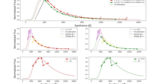
Figure 13: Comparison of the observed $grizJHKs$ SED one day after maximum light with blackbody models for our two tentative redshifts. Radii and temperature correspond to the best fit parameters. The black dotted line represents the linear absorption between 1500-3000 Å expected for a SLSN. The middle panels compare our observations and modelling with two SLSNe, SN 2015bn and SN 2006gy. The bottom panels present an SED at MJD = 57035.25 corresponding to the linear decay phase. It is clear that the blackbody assumption is not completely valid at these epochs.

Table 9: Bolometric information for UID 30901.

$z$	MJD peak bolometric	Peak bolometric luminosity	Bolometric linear decline rate	Total bolometric energy	Pseudo-bolometric luminosity
	(days)	(erg s-1)	(mag/100 days)	emitted (erg)	at MJD=57428.0 (erg s-1)
$0.37$	$56763.0$	$5.4(3)\times 10^{43}$	$1.12(01)$	$5.51\times 10^{50}$	$2.7(2)\times 10^{41}$
$0.53$	$56763.0$	$1.1(1)\times 10^{44}$	$1.25(01)$	$1.04\times 10^{51}$	$5.7(4)\times 10^{41}$

• Numbers in parenthesis correspond to 1-$\sigma$ statistical uncertainties.

3.6 Parametric Engine Models

In this section we implement two models that may be able to account for the high constrained energy of UID 30901: a spinning magnetar and the radioactive decay of ⁵⁶Ni.

3.6.1 Power injection from the spin-down of a magnetar

First developed by Maeda et al. (2007), Woosley (2010) and Kasen & Bildsten (2010), a rapidly rotating magnetar has been applied to Hydrogen-poor SLSNe providing a good fit to their light curves. Essentially, this model consists in the collapse of a massive star creating a rapidly spinning neutron star (P $\sim$ few milliseconds) with a strong magnetic field ($\sim$ 10¹⁴G). The magnetic dipole will decay in days or weeks emitting enough high-energy radiation to heat the ejecta and power its observed luminosity. The model has been modified to account for the diversity of SLSN light curves (Inserra et al., 2013; Wang et al., 2015; Nicholl et al., 2017).

The principal parameters of the magnetar model are: 1) the period of the magnetar and its magnetic field, which control the energy input of the SLSN; 2) the opacity and the high-energy opacity, which control the internal diffusion time and the high-energy "leakage" parameter (Wang et al., 2015); 3) the ejecta mass and the photospheric velocity, which control the kinetic energy and the radius of the photosphere; and 4) the final temperature and time of explosion. The evolution of the radius and temperature are controlled by simple rules (See Appendix A) and the SED is assumed to be a blackbody. The model does not account for the host galaxy reddening or the modified part of the blackbody. We implemented the magnetar model as described in Nicholl et al. (2017) and fitted it directly to the observed magnitudes. We fit our model with the emcee sampler (Foreman-Mackey et al., 2013). Further details of our model can be seen in the Appendix A.

Our model fit for $z=0.37$ predicts a period spin $P=5.8^{+0.5}_{-0.6}$ms, a magnetic field $B=1.3^{+0.3}_{-0.2}\times 10^{14}$G and an $M_{\mathrm{ej}}=12.0^{+5.3}_{-8.3}$ M_⊙. We also find the neutron star mass $M_{\mathrm{ns}}=1.9\pm 0.2$ M_⊙ and an ejecta velocity of $V_{\mathrm{ej}}=6387^{+217}_{-231}$km s^-1. For simplicity we consider a constant expansion of the ejecta and this velocity is consistent with the plateau of velocity at the tail of the light curves derived from the blackbody model. We also fit the opacity $\kappa$ and the opacity to high-energy photons $\kappa_{\gamma}$ parameters, that control the injection of energy from the magnetar, resulting in $\kappa=0.13\pm 0.05$ cm² gr^-1 and $\kappa_{\gamma}=0.10^{+0.07}_{-0.05}$ cm² gr^-1. The model predicts an explosion time $t_{0}=31.2^{+1.5}_{-1.6}$ days before the first detection, which is in disagreement with the upper limits found from non-detections. The outcome of our model for $z=0.37$ is shown in Figure 14.

A similar set of parameters are found for $z=0.53$. We notice that a higher $z$ implies hotter and faster ejecta, a faster spinning magnetar and a weaker magnetic field. Both set of parameters are consistent with the typical values calculated by Nicholl et al. (2017) for a sample of 38 SLSNe-I (See Figure 15). A full set of parameters for both redshifts is presented in Table 10.

3.6.2 Radioactive Decay of ⁵⁶Ni

Another theoretical mechanism to reproduce the extreme luminosities of SLSNe is through the radioactive decay of several solar masses of ⁵⁶Ni. The main parameters of this model are $M_{\mathrm{ej}}$ and $M_{\mathrm{Ni}}$, the masses of the ejecta and ⁵⁶Ni, respectively. Additional parameters include the ejecta velocity ($V_{\mathrm{ej}}$), final temperature ($T_{f}$) and the opacity ($\kappa$).

Our model predicts an ejecta mass of $M_{\mathrm{ej}}=5.8^{+3.3}_{-3.5}$ and a ⁵⁶Ni mass of $M_{\mathrm{Ni}}=4.3\pm 0.1$M_⊙, which is beyond the nickel mass to total mass ratio found by Umeda & Nomoto (2008).We estimate a final temperature $T_{f}=4911_{-62}^{+65}$ K which is fairly consistent with theoretical estimations to the photospheric temperature at this phase (Dessart et al., 2012). The resulting opacity is $\kappa=0.12^{+0.05}_{-0.07}$ cm² gr^-1, which is among the expected values for a SLSN powered by this model. This model predicts an explosion time $t_{0}=24^{+1.4}_{-1.5}$ days before the first detection, inconsistent with our non-detection point.

For $z=0.53$ our best fit predicts a $M_{\mathrm{Ni}}$ higher than the $M_{\mathrm{ej}}$, which is nonphysical. The model also implies a faster and hotter ejecta and an explosion time of $\sim 21.6$ days before explosion. The full set of parameters for both redshifts can be found in Table 10.

Model	Magnetar		56Ni
$z$	0.37	0.53	0.37	0.53
$\mathcal{M}_{{}^{56}Ni}$ [$M_{\odot}$]	–	–	4.3${}_{-0.1}^{+0.1}$	7.9${}_{-0.4}^{+0.3}$
$\mathcal{P}$ [$ms$]	5.8${}_{-0.6}^{+0.5}$	4.2${}_{-0.4}^{+0.4}$	–	–
$\mathcal{B}$ [1014 Gauss]	1.3${}_{-0.2}^{+0.3}$	1.0${}_{-0.2}^{+0.2}$	–	–
$\mathcal{M}_{ns}$ [$M_{\odot}$]	1.9${}_{-0.2}^{+0.2}$	1.9${}_{-0.2}^{+0.2}$	–	–
$\mathcal{M}_{ej}$ [$M_{\odot}$]	12.0${}_{-8.3}^{+5.3}$	11.6${}_{-4.7}^{+4.5}$	5.8${}_{-3.5}^{+3.3}$	6.3${}_{-4.4}^{+3.2}$
$\mathcal{V}_{ej}$ [$km/s$]	6387${}_{-231}^{+217}$	8303${}_{-293}^{+226}$	7130${}_{-240}^{+262}$	10310${}_{-392}^{+561}$
$\mathcal{K}$ [$cm^{2}/gr$]	0.13${}_{-0.05}^{+0.05}$	0.15${}_{-0.03}^{+0.04}$	0.12${}_{-0.07}^{+0.05}$	0.10${}_{-0.06}^{+0.04}$
$\mathcal{K}_{\gamma}$ [$cm^{2}/gr$]	0.10${}_{-0.05}^{+0.07}$	0.14${}_{-0.05}^{+0.06}$	–	–
$T$ [$Kelvin$]	4963${}_{-61}^{+57}$	5719${}_{-51}^{+72}$	4911${}_{-62}^{+65}$	5549${}_{-91}^{+80}$
$t_{exp}$ [$days$]	31.2${}_{-1.6}^{+1.5}$	31.4${}_{-1.6}^{+1.6}$	24.0${}_{-1.5}^{+1.4}$	21.6${}_{-1.7}^{+1.5}$

Table 10: Magnetar and ⁵⁶Ni Model Fit Results. The $t_{exp}$ is reported in observer frame

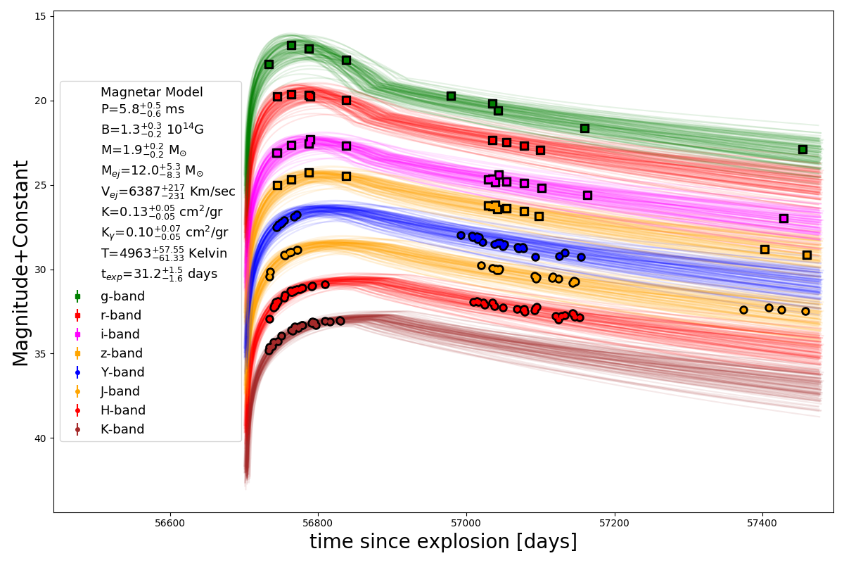
Figure 14: Magnetar model fit for $z=0.37$.

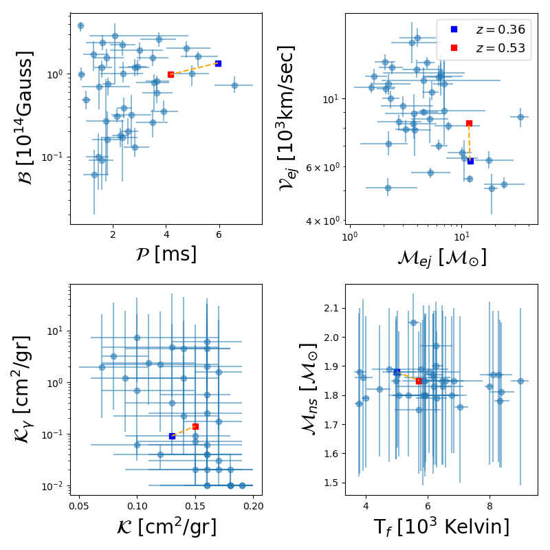
Figure 15: Comparison against the parameters measured by Nicholl et al. (2017). The blue and red squares represent the UID 30901 at $z=0.37$ and $z=0.53$. Our object present typical SLSNe values for both redshift. The period in the case of $z=0.37$ adopt an extreme value but still consistent with others SLSNe

4 Discussion

We divide this section in two parts. The first one presents a detailed analysis of the outcome parameters of our model fits for $z=0.37$, and how it changes when we assume $z=0.53$. Then we discuss the explosion epoch and the possibility that ejecta-CSM interaction as a power source for UID 30901.

In the second part of this section we analyse the light-time light curve flattening from two perspectives, first as a power source effect and then, as a light echo.

4.1 Fitting results

4.1.1 Power Source

In Section 3.6 we presented two models as the potential power source for UID 30901, radioactive decay of ⁵⁶Ni and the spin-down of a magnetar. Here we discuss the parameters resulting from these fits.

Explosions powered by the radioactive decay of ⁵⁶Ni are expected to dim at a rate of $\sim 1$ mag/100 days. Comparing this with the decay calculated in Sections 3.4.2 and 3.4.3, we note a difference in factors of 1.1 for $z=0.37$ and 1.5 for $z=0.53$ between the expected behaviour and the photometry in the final year. (See Table 9 and Figure 12). Ignoring the final year, the light curve declines faster than the expected ⁵⁶Ni radioactive decay but is still consistent with this kind of explosion (See Table 9). In fact, this model provides an excellent fit to first phases of the light curve.

For $z=0.37$ our model predicts that the $M_{\mathrm{Ni}}$ is $\sim$75% of the $M_{\mathrm{ej}}$, which is not consistent with theoretical studies (Umeda & Nomoto, 2008) or any other observation reported in the literature (e,g. Jerkstrand et al., 2016). For $z=0.53$ the $M_{\mathrm{Ni}}$ necessary to power the UID 30901 light curve is higher than the $M_{\mathrm{ej}}$. These very high $M_{\mathrm{Ni}}$ to $M_{\mathrm{ej}}$ ratios is the main reason to discard this model.

Dessart et al. (2012) present a model that predicts that the photosphere of a PISN is essentially cold, reaching temperatures of 6000 K at the peak. We derived a peak blackbody temperature ($T_{bb}\sim 12000$ K) which is not compatible with those predictions. At latter phases a similar behaviour is found. While the model predicts a maximum temperature of $\sim 4000$ K between 100-200 days after the peak, we estimate a temperature of $\sim 5000$ K at the same epochs. Nevertheless, it is important to mention that the blackbody modelling is not completely reliable at late epochs of the light curve.

The unphysically large values of $M_{\mathrm{Ni}}$, the inconsistent temperature predictions, and the difficulty of this model to reproduce the flattening strongly argue against ⁵⁶Ni decay as the main power source for UID 30901.

The second scenario is the spin-down of a magnetar. This model reproduces the complete light curve evolution and the best fit parameters are in good agreement with the values typically found in the literature.

From the first detection to $\sim$ 200 days, the resulting bolometric luminosity and temperatures values derived from the blackbody fit are consistent with those determined from the spin-down model. The main difference is the temperature at the nebular phase, where the resulting temperatures differ by 20%. This is expected since the blackbody assumption is no longer valid at these late epochs.

Our model predicts $M_{\mathrm{ej}}=11.9^{+4.8}_{-6.4}$ M_⊙, $B=1.4^{+0.3}_{-0.3}$ G and $P=6.0^{+0.6}_{-0.5}$ ms. These results are among the expected values for a SLSNe (See Figure 15). For $z=0.53$ the model yields in a weaker magnetic field, a slower spin period and a similar ejecta mass. It also gives a faster and hotter ejecta. The neutron star mass remains constant for both redshifts. A complete set of parameters is shown in Table 10

4.1.2 Explosion time

One of the parameters of our models is the explosion time t₀. We find that both the radioactive decay and the magnetar model predict explosion times in disagreement with the observations. The results are presented in Table 10.

The magnetar model has shown mixed results when estimating explosion times for other systems. While for SN 2015bn (Nicholl et al., 2016a) and SN 2016iet (Gomez et al., 2019) discrepancies between the observations and the explosion time are found, for SN 2017cgi (Fiore et al., 2021) fits a rise time consistent with observations and also with a fast-evolving SLSNe.

4.1.3 Circumstellar Interaction

Another potential scenario to explain the brightness of a SLSNe is the interaction between the SN ejecta with the CSM. The progenitor may be surrounded by CSM ejected from the progenitor itself before the explosion. Afterwards, the SN ejecta will collide with this material, and by converting the kinetic energy of the ejecta into radiative energy, can power the luminosity of the SN. This interaction can be responsible for bumps or wiggles in the light curves of some SLSNe (Yan et al., 2015).

Unlike the double-peaked light curve of iPTF13ehe (Yan et al., 2015), the UID 30901 light curve does not show any strong observational signature of the interaction between the ejecta and CSM.

Spectral features are the main evidence for interaction with the CSM, as seen in SN 2006gy (Jerkstrand et al., 2020). Because of the lack of spectra at the photospheric phase, we cannot test for the presence of any H$\alpha$ broad line to confirm the ejecta-CSM interaction. However, a strong interaction should leave an imprint in the SED, visible as a deviation from the blackbody model. A close inspection of the SED at individual epochs of the early and post peak phases (see Figure 13) shows that the photometry is in good agreement with a blackbody model, and therefore the presence of a strong H$\alpha$ broad line is unlikely. In Section 3.3.2 we found that the late-time SED of UID 30901 looks very similar to that of SN 2018bsz, which hints at the presence of CSM interaction at these phases. However, this late event clearly cannot be responsible for the initial power injection for UID 30901 but instead it would correspond to a possible late evolution.

In summary, we cannot rule out some ejecta-CSM interaction, but under the criteria outlined above, there is no evidence that this mechanism was the main power source for UID 30901.

4.2 Flattening

One of the features of the UID 30901 light curves is the flattening at late epochs (see Section 3.4.3), which is especially clear in the $g$-band at +500 days after the explosion (see Figure 2). In this section we approach this phenomena from two different perspectives. The first one is associated to the power source. While the magnetar and CSM models could explain the flattening, the constant decline rate of radioactive decay of ⁵⁶Ni cannot explain this behaviour.

Another option to explain the flattening is a light echo. To study that case, we compare the color at the peak with the color at the nebular phase.

4.2.1 Flattening as a power source effect

As is presented in Section 4.1.1, the magnetar model can reproduce the complete light curve evolution for both possible redshifts of UID 30901, and the outcome parameters are in good agreement with the literature and with those obtained from the blackbody modelling.

In the case of CSM interaction, it is more difficult to conclude. Assuming an ejecta expanding with a velocity between $4000-10000$ km s^-1, a shell of matter located at $r\sim 1-4\times 10^{16}$ cm could flatten the slope of the light curve leaving also an imprint in the spectra. Without spectroscopic data, we cannot discard the existence of such interaction, but as we discuss in Section 4.1.3 we conclude that it is unlikely for this model to be the main power source and therefore is also unlikely to be the responsible of the change in light curve decay rate.

4.2.2 Light Echo

Light echoes occur when light emitted at early phases of the SN is reflected by dust and observed at later times. While electron scattering is achromatic, dust scattering is efficient in reflecting blue light so the color at the echo phase should be as blue as the peak, as we are observing the same light, but reflected some time later in the line of sight. Light echoes have been observed in SNe II (Crotts, 1988; Suntzeff et al., 1988) and also, late observations of SN 2006gy have been interpreted as a light echo (Miller et al., 2010).

To study this possibility, we compare the color at the peak with the color at the nebular phase in every band where data are available ($gizYJ$), and where the last detections of $z$ and $J$ are the linear interpolation of the late epochs described in Section 3.4.3.

We measured a color $(g-i)_{p}=0.08\pm 0.003$ at the peak, which is not consistent with the red color observed in the last datapoint of $(g-i)_{l}=1.93\pm 0.013$. A similar case occurs with $(g-z)$, $(g-y)$ and $(g-J)$. A smaller difference, but still inconsistent when comparing the early and late photometry is found in the $(i-J)$, $(z-J)$ and $(y-J)$ colors.

A different scenario occurs in $izy$ bands. For $(i-z)$ we found similar values between the peak and the nebular phase and found a bluer color at the nebular phase for $(i-y)$ and $(z-y)$. We associate this behaviour to the presence of emission lines typical of a nebular spectra at the $izy$ bands. Without spectra at these epochs we cannot identify which lines might be present, but based on the possible values of $z$ for UID 30901, we can discard a strong late-H$\alpha$ emission.

In summary, the discrepancy between the maximum light and late phase colours in many filter-pairs is sufficient to discard a light echo as the responsible mechanism to explain of the flattening of the light curves.

Table 11: Color and color difference between peak and tail of the UID 30901 in different photometric filters.

Bands	Color at peak	Color at tail	$\Delta_{color}$
	MJD $\sim$ 56764	MJD $\sim$ 57450
	(mag)	(mag)	(mag)
$(g-i)$	0.08 (0.003)	1.93 (0.01)	-1.85 (0.02)
$(g-z)$	0.06 (0.02)	1.77 (0.06)	-1.71 (0.09)
$(g-y)$	-0.16 (0.02)	1.45 (0.04)	-1.61 (0.01)
$(g-j)$	-0.23 (0.02)	2.43 (0.03)	-2.66 (0.05)
$(i-z)$	-0.02 (0.03)	-0.0 (0.1)	-0.0 (0.1)
$(i-y)$	-0.25 (0.03)	-0.48 (0.02)	0.231 (0.002)
$(i-j)$	-0.31 (0.02)	0.57 (0.03)	-0.88 (0.05)
$(z-y)$	-0.23 (0.001)	-0.5 (0.1)	0.2 (0.1)
$(z-j)$	-0.29 (0.002)	0.52 (0.06)	-0.81 (0.06)
$(y-j)$	-0.07 (0.003)	0.98 (0.07)	-1.05 (0.07)

5 Summary

We have presented multi-wavelength photometry for UID 30901, a new SLSN discovered in the COSMOS field by the NIR UltraVISTA SN Survey. Even though the UltraVISTA project was not aimed for the search of transients, its depth and high cadence plus the high quality of the achieved photometry make this survey optimal for a transient search.

We complement the NIR data with photometry from DECam ($griz$) and SUBARU-HSC ($grizy$). This allows us to have a wide wavelength coverage that makes the UID 30901 one of the best observed SLSN to date. This wide coverage let us compare the photometry with spectra available in the literature. The data show that UID 30901 belongs to the "sub-luminous" family of SLSNe, reaching a peak apparent magnitude of -20 or more in all observed bands, making it hard to be observed by other surveys such as PTF.

Analysis of the light curves show that the object peaks later at longer effective wavelengths, similar to SNe Ic and Ic-BL. Similarities between these two kind of objects has been seen before, finding that even though they are different classes, there is an overlap in their peak magnitudes among the brighter Ic and the low luminosity SLSNe.

To determine the explosion time we applied two simple fits to the rise phase of the light curves, a linear polynomial and a power law. The last one provides an explosion time constraint which differs by $\sim 10$ days with the linear fit but which is in better agreement with a non-detection in the $H$-band five days before the fist detection of the SN. We note that the NIR light curve shape at rise phase can be reproduced by a power law with $\alpha\sim 0.7$, an odd value compared with the typical $\alpha$ found for other SNe. However, there are no systematic studies that explore SLSNe in the NIR in order to establish a correlation between the rise phase and power law fits.

We detect the host of UID 30901 in a deep HST F814W image. The host is identified as a faint, dwarf galaxy most likely characterised by a small stellar mass and low SFR, placing it at the extreme of the properties of SLSN hosts, as determined by Perley et al. (2016). Since we have no spectra for neither the host nor the SN, we adopt the photometric-$z$ values provided by the COSMOS2015 catalog for possible nearby companions, identified as galaxies A and B, with values $z$ = 0.37 and $z$ = 0.53, respectively.

Despite the lack of spectra, we were able to reconstruct the SEDs for individual epochs at different phases of the light curve evolution. The early phases yielded the most reliable SEDs. Following the assumption that SLSNe radiate as a blackbody we estimated the radius and temperature evolution and a bolometric and pseudo-bolometric light curves. Since it is known that below $\sim 3000$ Å  the SED of a SLSN suffers from significant absorption and our blackbody modelling for $z>1$ implies that most of the emission would have occurred in the near and far UV, we were able to discard a high $z$ value for UID 30901.

We explored the most common power sources for SLSNe and applied these physical models to our source. The high ⁵⁶Ni masses necessary to power this SLSNe and, to a lesser extent, the estimated high temperatures at the peak lead us to discard the radioactive decay as the main power source for the UID 30901.

We consider that there is no strong physical reasons to model this object as an ejecta-CSM interacting SLSN. The smoothness of the light curve, absence of early bumps and the lack of signs of interaction of the individual SEDs makes it very unlikely for this option to be the main power source.

In the case of the spin-down magnetar model, we found that it provides an excellent fit and typical values for all parameters. Our model predicts a magnetic field $B\approx 1.3\times 10^{14}$ G, a period spin $P\approx 5.8$ ms and ejecta mass of $M_{\mathrm{ej}}\approx 12.0$ M_☉ for $z=0.37$. For $z=0.53$ we found $B\approx 1.0\times 10^{14}$ G, $P\approx 4.2$ ms, M${}_{ej}\approx 11.6$ M_⊙. In both cases these physical parameters place our object as a typical SLSNe. The main drawback of the magnetar model is that it overestimates the explosion time $t_{0}$, in contradiction with observed constraints.

6 Acknowledgements

Based on data products from observations made with ESO Telescopes at the La Silla Paranal Observatory under ESO programme ID 179.A-2005 and on data products produced by CALET and the Cambridge Astronomy Survey Unit on behalf of the UltraVISTA consortium.

This research uses services or data provided by the Astro Data Archive at NSF’s National Optical-Infrared Astronomy Research Laboratory. NSF’s OIR Lab is operated by the Association of Universities for Research in Astronomy (AURA), Inc. under a cooperative agreement with the National Science Foundation.

Data Availability

The photometric data of UID 30901 is included in the Appendix B of this article. It also can be found in the online supplementary material and is available on the CDS VizieR facility.

Appendix A Magnetar Fit

Our simplified Magnetar model is based on Nicholl et al. (2017)’s model. Where the following quantities are defined as:

$$E_{mag}=\frac{1}{2}I\omega^{2}=2.6\times 10^{52}\left(\frac{M_{NS}}{1.4M_{\odot}}\right)^{\frac{3}{2}}\left(\frac{P}{1ms}\right)^{-2}erg$$ (1)

is the rotational energy available from the neutron star.

$$t_{mag}\approx\frac{P}{2\dot{P}}=1.3\times 10^{5}\left(\frac{M_{NS}}{1.4M_{\odot}}\right)^{\frac{3}{2}}\left(\frac{P}{1ms}\right)^{2}\left(\frac{B_{\perp}}{10^{14}G}\right)^{-2}s$$ (2)

is the spin-down timescale. Both expression give the dipole radiation power:

$$F(t)=\frac{E_{mag}}{t_{mag}}\frac{1}{(1-t/t_{mag})^{2}}$$ (3)

This power is input into the ejecta where most of it is thermalized and re-emitted by the SN as derived by Arnett (1982):

$$L(t)=2e^{-(t/t_{diff})^{2}}(1-e^{-A/t^{2}})\int_{0}^{t}F(t^{\prime})\left(\frac{t^{\prime}}{t_{diff}}\right)e^{(t^{\prime}/t_{diff})^{2}}\frac{dt^{\prime}}{t_{diff}}$$ (4)

where the diffusion time $t_{diff}$ is:

$$t_{diff}=\left(\frac{2\kappa M_{ej}}{\beta cV_{ej}}\right)^{\frac{1}{2}}$$ (5)

and the “leakage” parameter introduced by Wang et al. (2015) that allows some of the high energy escape through the ejecta is:

$$A=\frac{3\kappa_{\gamma}M_{ej}}{4\pi V_{ej}^{2}}$$ (6)

A set of simple and empirically motivated rules control Radius and Temperature of the blackbody through the time:

$$\Delta=\left(\frac{L(t)}{4\pi\sigma v_{phot}^{2}t^{2}}\right)^{\frac{1}{4}}$$ (7)

$$T_{phot}(t)=\begin{cases}\Delta&\text{if }\Delta>T_{f}\\ T_{f}&\text{if }\Delta\leq T_{f}\\ \end{cases}$$ (8)

$$R_{phot}(t)=\begin{cases}v_{phot}t&\text{if }\Delta>T_{f}\\ \left(\frac{L(t)}{4\pi\sigma T_{f}^{4}}\right)^{\frac{1}{2}}&\text{if }\Delta\leq T_{f}\\ \end{cases}$$ (9)

where the $T_{f}$ is the final temperature reached by the blackbody, typically between 4000 and 7000 K (Nicholl et al., 2017). From the blackbody Radius and Temperature the photometry is estimated for the different bandpasses (considering the redshift) and compared to the observed photometry. We simultaneously fitted all the model’s parameters maximizing the likelihood $\mathcal{L}$:

$$ln(\mathcal{L})=-\frac{1}{2}\sum{\left[\frac{O_{i}-M_{i}}{\sigma_{i}^{2}+\sigma^{2}}+ln(\sigma_{i}^{2}+\sigma^{2})\right]}$$ (10)

where $O_{i},\sigma_{i}$ are the photometry values and errors, $M_{i}$ is the corresponding model value, and $\sigma$ is an additional error value to control underestimation of the photometry errorbars. To compute the best fit parameter values we use the emcee package (Foreman-Mackey et al., 2013).

Appendix B Photometry

Table 12: UltraVISTA NIR Photometry of UID 30901.

Date UT	MJD	$Y$	$J$	$H$	$K_{s}$
2014-03-17	$56733.13$	–	–	–	$22.815$($0.143$)
2014-03-18	$56734.12$	–	$22.472$($0.061$)	$22.958$($0.143$)	$22.614$($0.099$)
2014-03-19	$56735.11$	–	$22.158$($0.051$)	–	$22.652$($0.159$)
2014-03-22	$56738.13$	–	–	–	$22.554$($0.132$)
2014-03-24	$56740.08$	–	–	$22.296$($0.084$)	$22.313$($0.124$)
2014-03-25	$56741.10$	–	–	$22.152$($0.075$)	–
2014-03-26	$56742.04$	–	–	$22.219$($0.090$)	–
2014-03-27	$56743.06$	–	–	$21.960$($0.072$)	–
2014-03-28	$56744.07$	$21.555$($0.043$)	–	$22.038$($0.076$)	–
2014-03-29	$56745.13$	$21.482$($0.043$)	–	–	–
2014-03-30	$56746.08$	$21.385$($0.045$)	–	$21.896$($0.103$)	$22.291$($0.113$)
2014-04-02	$56749.16$	$21.316$($0.039$)	–	–	–
2014-04-03	$56750.04$	$21.250$($0.036$)	–	–	$21.962$($0.083$)
2014-04-04	$56751.08$	$21.232$($0.039$)	–	–	–
2014-04-07	$56754.08$	$21.131$($0.038$)	$21.177$($0.043$)	$21.716$($0.068$)	–
2014-04-08	$56755.08$	–	$21.219$($0.042$)	$21.535$($0.043$)	–
2014-04-14	$56761.08$	–	$21.049$($0.040$)	–	–
2014-04-16	$56763.15$	–	$21.004$($0.038$)	$21.298$($0.045$)	–
2014-04-17	$56764.06$	–	$20.973$($0.041$)	$21.360$($0.046$)	$21.596$($0.078$)
2014-04-18	$56765.02$	–	–	$21.360$($0.044$)	–
2014-04-19	$56766.04$	–	–	$21.316$($0.044$)	$21.667$($0.082$)
2014-04-20	$56767.05$	$20.913$($0.044$)	–	$21.286$($0.043$)	$21.497$($0.039$)
2014-04-21	$56768.03$	–	–	$21.255$($0.044$)	$21.424$($0.051$)
2014-04-22	$56769.02$	–	–	$21.222$($0.036$)	–
2014-04-24	$56771.07$	$20.768$($0.038$)	$20.884$($0.039$)	$21.204$($0.036$)	–
2014-04-25	$56772.07$	–	$20.858$($0.040$)	–	–
2014-04-25	$56772.96$	–	–	–	$21.491$($0.041$)
2014-04-27	$56774.03$	–	–	–	$21.424$($0.039$)
2014-04-27	$56774.98$	–	–	$21.191$($0.050$)	–
2014-05-01	$56778.03$	–	–	$21.096$($0.040$)	$21.341$($0.045$)
2014-05-02	$56779.04$	–	–	$21.126$($0.044$)	$21.331$($0.047$)
2014-05-13	$56790.99$	–	–	$21.011$($0.064$)	$21.216$($0.050$)
2014-05-15	$56792.02$	–	–	$21.005$($0.042$)	$21.123$($0.029$)
2014-05-16	$56793.97$	–	–	–	$21.201$($0.047$)
2014-05-18	$56795.01$	–	–	–	$21.142$($0.049$)
2014-05-19	$56796.98$	–	–	–	$21.325$($0.042$)
2014-05-31	$56808.99$	–	–	$20.889$($0.049$)	$21.081$($0.046$)
2014-06-08	$56816.00$	–	–	–	$21.093$($0.048$)
2014-06-20	$56829.00$	–	–	–	$21.049$($0.056$)
2014-06-21	$56829.97$	–	–	–	$21.066$($0.047$)
2014-12-01	$56992.32$	$21.988$($0.045$)	–	–	–
2014-12-16	$57007.27$	$22.056$($0.046$)	–	–	–
2014-12-17	$57008.25$	$22.131$($0.045$)	–	–	–
2014-12-18	$57009.27$	–	–	$21.952$($0.048$)	–
2014-12-23	$57014.28$	$22.097$($0.045$)	–	$21.907$($0.045$)	–
2014-12-24	$57015.23$	$22.260$($0.059$)	–	–	–
2014-12-25	$57016.26$	–	–	$21.945$($0.045$)	–
2014-12-26	$57017.29$	$22.136$($0.048$)	–	–	–
2014-12-29	$57020.22$	–	$21.798$($0.075$)	–	–
2014-12-31	$57022.24$	$22.402$($0.092$)	–	–	–
2015-01-01	$57023.20$	–	–	$22.001$($0.087$)	–
2015-01-03	$57025.22$	–	–	$22.112$($0.104$)	–
2015-01-13	$57035.31$	–	$21.969$($0.052$)	$21.979$($0.107$)	–
2015-01-16	$57038.29$	$22.539$($0.063$)	–	$22.214$($0.058$)	–
2015-01-18	$57040.31$	–	$22.005$($0.040$)	–	–
2015-01-19	$57041.33$	–	$22.078$($0.057$)	–	–
2015-01-21	$57043.29$	$22.459$($0.058$)	$22.082$($0.114$)	–	–
2015-01-22	$57044.33$	–	$21.986$($0.064$)	–	–
2015-01-23	$57045.26$	$22.441$($0.054$)	–	–	–
2015-01-27	$57049.22$	$22.671$($0.077$)	–	$22.301$($0.071$)	–
2015-01-29	$57051.18$	$22.537$($0.052$)	–	–	–

• Numbers in parenthesis correspond to 1 $\sigma$ statistical uncertainties.

Table 13: continued

UltraVISTA NIR Photometry of UID 30901. Date UT MJD $Y$ $J$ $H$ $K_{s}$ 2015-02-15 $57068.18$ – – $22.383$($0.069$) – 2015-02-16 $57069.10$ $22.721$($0.057$) – – – 2015-02-17 $57070.18$ $22.775$($0.054$) – – – 2015-02-18 $57071.18$ $22.779$($0.092$) – – – 2015-02-23 $57076.14$ $22.712$($0.049$) – – – 2015-02-24 $57077.14$ $22.782$($0.049$) – $22.419$($0.111$) – 2015-02-25 $57078.06$ – – $22.373$($0.083$) – 2015-02-26 $57079.09$ – – $22.532$($0.136$) – 2015-03-11 $57092.20$ – $22.396$($0.117$) $22.469$($0.104$) – 2015-03-12 $57093.14$ $23.296$($0.171$) – $22.314$($0.077$) – 2015-03-13 $57094.09$ – $22.570$($0.114$) – – 2015-03-14 $57095.06$ – $22.486$($0.092$) $22.246$($0.093$) – 2015-04-04 $57116.09$ – $22.541$($0.054$) – – 2015-04-05 $57117.06$ – $22.457$($0.075$) – – 2015-04-09 $57121.14$ – – $22.787$($0.174$) – 2015-04-12 $57124.07$ – $22.595$($0.073$) $22.971$($0.159$) – 2015-04-13 $57125.13$ $23.252$($0.188$) – – – 2015-04-16 $57128.03$ – – $22.774$($0.137$) – 2015-04-21 $57133.05$ $23.025$($0.217$) – $22.723$($0.125$) – 2015-05-01 $57143.06$ – $22.846$($0.103$) $22.611$($0.165$) – 2015-05-02 $57144.03$ – $22.790$($0.077$) $22.660$($0.139$) – 2015-05-03 $57145.10$ – $22.702$($0.082$) – – 2015-05-04 $57146.01$ – – $22.842$($0.125$) – 2015-05-05 $57147.09$ – $22.739$($0.116$) – – 2015-05-11 $57153.09$ – – $22.847$($0.170$) – 2015-05-13 $57155.05$ $23.283$($0.173$) – – – 2015-12^a $57374.10$ – $24.399$($0.127$) – – 2016-01^a $57408.76$ – $24.289$($0.092$) – – 2016-02^a $57425.34$ – $24.425$($0.156$) – – 2016-03^a $57457.94$ – $24.488$($0.138$) – –

• Numbers in parenthesis correspond to 1 $\sigma$ statistical uncertainties.

• ^aThe $J$-band photometry was computed from an average image made of several frames co-added obtained over the month.

Table 14: Optical photometry of UID 30901

Date UT	MJD	$g$	$r$	$i$	$z$	$y$	Tel.
2014-03-17	$56733.14$	$21.911$($0.125$)	–	–	–	–	1
2014-03-25	$56741.47$	–	–	–	–	$21.547$($0.015$)	2
2014-03-26	$56742.98$	–	–	$21.120$($0.039$)	–	$21.488$($0.013$)	2
2014-03-28	$56744.35$	–	$20.922$($0.024$)	–	$21.060$($0.018$)	–	2
2014-03-28	$56744.51$	–	–	$21.141$($0.020$)	–	–	2
2014-04-03	$56750.29$	–	–	–	–	$21.015$($0.020$)	2
2014-04-17	$56764.06$	$20.790$($0.021$)	$20.679$($0.017$)	$20.679$($0.018$)	$20.688$($0.043$)	–	1
2014-05-09	$56786.97$	$20.998$($0.130$)	$20.744$($0.185$)	$20.587$($0.153$)	$20.287$($0.187$)	–	1
2014-05-11	$56788.97$	–	$20.792$($0.150$)	$20.350$($0.075$)	–	–	1
2014-06-29	$56837.96$	$21.662$($0.098$)	$21.016$($0.087$)	$20.725$($0.121$)	$20.513$($0.122$)	–	1
2014-11-18	$56979.62$	$23.777$($0.033$)	–	–	–	$21.727$($0.015$)	2
2015-01-07	$57029.27$	–	–	$22.718$($0.087$)	$22.261$($0.093$)	–	1
2015-01-13	$57035.26$	$24.251$($0.149$)	$23.404$($0.055$)	$22.691$($0.036$	$22.305$($0.054$)	–	1
2015-01-17	$57039.05$	–	–	$22.876$($0.023$)	$22.215$($0.046$)	–	2
2015-01-19	$57041.00$	–	–	–	$22.465$($0.031$)	$22.259$($0.013$)	2
2015-01-20	$57042.46$	$24.646$($0.020$)	–	–	–	–	2
2015-01-21	$57043.66$	–	–	$22.432$($0.070$)	–	–	2
2015-01-27	$57049.65$	–	–	–	–	$22.371$($0.015$)	2
2015-02-01	$57054.29$	–	$23.502$($0.106$)	$22.853$($0.048$)	$22.436$($0.070$	–	1
2015-02-25	$57078.12$	–	$23.735$($0.185$)	$22.935$($0.096$)	$22.568$($0.092$)	–	1
2015-03-16	$57097.44$	–	–	–	$22.857$($0.033$)	–	2
2015-03-18	$57099.45$	–	$23.967$($0.037$)	–	–	–	2
2015-03-20	$57101.39$	–	–	$23.201$($0.070$)	–	–	2
2015-05-17	$57159.31$	$25.712$($0.078$)	–	–	–	–	2
2015-05-21	$57163.30$	–	–	$23.644$($0.066$)	–	–	2
2016-01-15	$57402.67$	–	–	–	$24.852$($0.111$)	–	2
2016-02-10	$57428.00$	–	–	$25.009$($0.183$)	–	–	2
2016-02-22	$57440.00$	–	–	–	–	$25.456$($0.207$)	2
2016-03-07	$57454.33$	$26.965$($0.170$)	–	–	–	–	2
2016-03-12	$57459.47$	–	–	–	$25.156$($0.105$)	–	2

• Numbers in parenthesis correspond to 1 $\sigma$ statistical uncertainties.

• Instrument/Telescope: 1=DECam/Blanco; 2=HSC/SUBARU.

Table 15: $grizy$ photometry of the local sequence stars around UID 30901.

	RA	Dec	$g$	$r$	$i$	$z$	$y$	SDSS IDa
1	49.84732	2.07194	$16.825$($0.004$)	$16.430$($0.005$)	$16.290$($0.005$)	$16.253$($0.009$)	–	272
2	49.83740	2.08621	$19.540$($0.013$)	$18.701$($0.010$)	$18.372$($0.010$)	$18.101$($0.028$)	$18.100$($0.001$)	377
3	49.83134	2.07922	$21.057$($0.039$)	$20.490$($0.034$)	$20.332$($0.042$)	$20.109$($0.150$)	$20.250$($0.001$)	813
4	49.82604	2.06618	$19.358$($0.012$)	$18.941$($0.011$)	$18.759$($0.013$)	$18.788$($0.048$)	$18.700$($0.001$)	369
5	49.83355	2.05832	$20.793$($0.031$)	$19.430$($0.015$)	$18.449$($0.011$)	$17.939$($0.025$)	$17.780$($0.001$)	431
6	49.83622	2.05565	$22.366$($0.112$)	$21.673$($0.086$)	$21.296$($0.094$)	$21.361$($0.426$)	$21.130$($0.001$)	818
7	49.81610	2.03973	$23.981$($0.381$)	$23.161$($0.351$)	$21.209$($0.095$)	$20.706$($0.230$)	$20.760$($0.002$)	982

• Numbers in parenthesis correspond to 1 $\sigma$ statistical uncertainties.

• ^aThe first 6 stars have SDSS ID prefixed by 1237651753997107. The 7th star SDSS ID is prefixed by 1237653664721928.

References

- Aihara et al. (2019) Aihara H., et al., 2019, PASJ, 71, 114
- Alard (2000) Alard C., 2000, A&AS, 144, 363
- Albareti et al. (2017) Albareti F. D., et al., 2017, ApJS, 233, 25
- Anderson et al. (2014) Anderson J. P., et al., 2014, ApJ, 786, 67
- Anderson et al. (2018) Anderson J. P., et al., 2018, A&A, 620, A67
- Angus et al. (2016) Angus C. R., Levan A. J., Perley D. A., Tanvir N. R., Lyman J. D., Stanway E. R., Fruchter A. S., 2016, MNRAS, 458, 84
- Angus et al. (2019) Angus C. R., et al., 2019, MNRAS, 487, 2215
- Arnett (1982) Arnett W. D., 1982, ApJ, 253, 785
- Barkat et al. (1967) Barkat Z., Rakavy G., Sack N., 1967, Phys. Rev. Lett., 18, 379
- Bertin et al. (2002) Bertin E., Mellier Y., Radovich M., Missonnier G., Didelon P., Morin B., 2002, in Bohlender D. A., Durand D., Handley T. H., eds, Astronomical Society of the Pacific Conference Series Vol. 281, Astronomical Data Analysis Software and Systems XI. p. 228
- Blanchard et al. (2021) Blanchard P. K., Berger E., Nicholl M., Chornock R., Gomez S., Hosseinzadeh G., 2021, arXiv e-prints, p. arXiv:2105.03475
- Capak et al. (2007) Capak P., et al., 2007, ApJS, 172, 99
- Cardelli et al. (1989) Cardelli J. A., Clayton G. C., Mathis J. S., 1989, ApJ, 345, 245
- Cartier et al. (2021) Cartier R., et al., 2021, arXiv e-prints, p. arXiv:2108.09828
- Chatzopoulos et al. (2013) Chatzopoulos E., Wheeler J. C., Vinko J., Horvath Z. L., Nagy A., 2013, ApJ, 773, 76
- Chen et al. (2021) Chen T. W., et al., 2021, arXiv e-prints, p. arXiv:2109.07942
- Conroy & Gunn (2010) Conroy C., Gunn J. E., 2010, ApJ, 712, 833
- Conroy et al. (2009) Conroy C., Gunn J. E., White M., 2009, ApJ, 699, 486
- Crotts (1988) Crotts A. P. S., 1988, ApJ, 333, L51
- Dalton et al. (2006) Dalton G. B., et al., 2006, in Society of Photo-Optical Instrumentation Engineers (SPIE) Conference Series. p. 62690X, doi:10.1117/12.670018
- De Cia et al. (2018) De Cia A., et al., 2018, ApJ, 860, 100
- Dessart et al. (2012) Dessart L., Hillier D. J., Waldman R., Livne E., Blondin S., 2012, MNRAS, 426, L76
- Dexter & Kasen (2013) Dexter J., Kasen D., 2013, ApJ, 772, 30
- Emerson & Sutherland (2010) Emerson J. P., Sutherland W. J., 2010, in Ground-based and Airborne Telescopes III. p. 773306, doi:10.1117/12.857105
- Emerson et al. (2006) Emerson J., McPherson A., Sutherland W., 2006, The Messenger, 126, 41
- Filippenko (1997) Filippenko A. V., 1997, ARA&A, 35, 309
- Fiore et al. (2021) Fiore A., et al., 2021, MNRAS, 502, 2120
- Firth et al. (2015) Firth R. E., et al., 2015, MNRAS, 446, 3895
- Flaugher et al. (2015) Flaugher B., et al., 2015, AJ, 150, 150
- Folatelli et al. (2010) Folatelli G., et al., 2010, AJ, 139, 120
- Foreman-Mackey et al. (2013) Foreman-Mackey D., Hogg D. W., Lang D., Goodman J., 2013, PASP, 125, 306
- Gal-Yam (2012) Gal-Yam A., 2012, Science, 337, 927
- Gal-Yam (2019) Gal-Yam A., 2019, ARA&A, 57, 305
- Gal-Yam et al. (2009) Gal-Yam A., et al., 2009, Nature, 462, 624
- Gezari et al. (2009) Gezari S., et al., 2009, ApJ, 690, 1313
- Gomez et al. (2019) Gomez S., et al., 2019, ApJ, 881, 87
- Guillochon et al. (2018) Guillochon J., Nicholl M., Villar V. A., Mockler B., Narayan G., Mandel K. S., Berger E., Williams P. K. G., 2018, ApJS, 236, 6
- Hamuy et al. (2006) Hamuy M., et al., 2006, PASP, 118, 2
- Heger & Woosley (2002) Heger A., Woosley S. E., 2002, ApJ, 567, 532
- Hunter et al. (2009) Hunter D. J., et al., 2009, A&A, 508, 371
- Ilbert et al. (2009) Ilbert O., et al., 2009, ApJ, 690, 1236
- Inserra et al. (2013) Inserra C., et al., 2013, ApJ, 770, 128
- Inserra et al. (2018) Inserra C., et al., 2018, MNRAS, 475, 1046
- Jerkstrand et al. (2016) Jerkstrand A., Smartt S. J., Heger A., 2016, MNRAS, 455, 3207
- Jerkstrand et al. (2017) Jerkstrand A., et al., 2017, ApJ, 835, 13
- Jerkstrand et al. (2020) Jerkstrand A., Maeda K., Kawabata K. S., 2020, Science, 367, 415
- Kasen & Bildsten (2010) Kasen D., Bildsten L., 2010, ApJ, 717, 245
- Kasen et al. (2011) Kasen D., Woosley S. E., Heger A., 2011, ApJ, 734, 102
- Laigle et al. (2016) Laigle C., et al., 2016, ApJS, 224, 24
- Leloudas et al. (2015) Leloudas G., et al., 2015, MNRAS, 449, 917
- Liu et al. (2017) Liu Y.-Q., Modjaz M., Bianco F. B., 2017, ApJ, 845, 85
- Lunnan et al. (2014) Lunnan R., et al., 2014, ApJ, 787, 138
- Lunnan et al. (2018) Lunnan R., et al., 2018, ApJ, 852, 81
- Maeda et al. (2007) Maeda K., et al., 2007, ApJ, 666, 1069
- Margutti et al. (2018) Margutti R., et al., 2018, ApJ, 864, 45
- Mazzali et al. (2016) Mazzali P. A., Sullivan M., Pian E., Greiner J., Kann D. A., 2016, MNRAS, 458, 3455
- Mazzali et al. (2019) Mazzali P. A., Moriya T. J., Tanaka M., Woosley S. E., 2019, MNRAS, 484, 3451
- McCracken et al. (2012) McCracken H. J., et al., 2012, A&A, 544, A156
- Milisavljevic et al. (2013) Milisavljevic D., et al., 2013, ApJ, 770, L38
- Miller et al. (2009) Miller A. A., et al., 2009, ApJ, 690, 1303
- Miller et al. (2010) Miller A. A., Smith N., Li W., Bloom J. S., Chornock R., Filippenko A. V., Prochaska J. X., 2010, AJ, 139, 2218
- Moriya et al. (2018) Moriya T. J., Sorokina E. I., Chevalier R. A., 2018, Space Sci. Rev., 214, 59
- Neill et al. (2011) Neill J. D., et al., 2011, ApJ, 727, 15
- Nicholl et al. (2016a) Nicholl M., et al., 2016a, ApJ, 826, 39
- Nicholl et al. (2016b) Nicholl M., et al., 2016b, ApJ, 828, L18
- Nicholl et al. (2017) Nicholl M., Guillochon J., Berger E., 2017, ApJ, 850, 55
- Nicholl et al. (2018) Nicholl M., et al., 2018, ApJ, 866, L24
- Nicholl et al. (2019) Nicholl M., Berger E., Blanchard P. K., Gomez S., Chornock R., 2019, ApJ, 871, 102
- Ofek et al. (2007) Ofek E. O., et al., 2007, ApJ, 659, L13
- Ørum et al. (2020) Ørum S. V., Ivens D. L., Strandberg P., Leloudas G., Man A. W. S., Schulze S., 2020, A&A, 643, A47
- Pastorello et al. (2010) Pastorello A., et al., 2010, ApJ, 724, L16
- Perley et al. (2016) Perley D. A., et al., 2016, ApJ, 830, 13
- Pignata et al. (2011) Pignata G., et al., 2011, ApJ, 728, 14
- Quimby et al. (2011) Quimby R. M., et al., 2011, Nature, 474, 487
- Quimby et al. (2018) Quimby R. M., et al., 2018, ApJ, 855, 2
- Rakavy & Shaviv (1967) Rakavy G., Shaviv G., 1967, ApJ, 148, 803
- Schlafly & Finkbeiner (2011) Schlafly E. F., Finkbeiner D. P., 2011, ApJ, 737, 103
- Schlegel (1990) Schlegel E. M., 1990, MNRAS, 244, 269
- Schulze et al. (2018) Schulze S., et al., 2018, MNRAS, 473, 1258
- Smith et al. (2007) Smith N., et al., 2007, ApJ, 666, 1116
- Smith et al. (2016) Smith M., et al., 2016, ApJ, 818, L8
- Smith et al. (2018) Smith M., et al., 2018, ApJ, 854, 37
- Steinhardt et al. (2014) Steinhardt C. L., et al., 2014, ApJ, 791, L25
- Stetson (1987) Stetson P. B., 1987, PASP, 99, 191
- Stritzinger et al. (2018a) Stritzinger M. D., et al., 2018a, A&A, 609, A134
- Stritzinger et al. (2018b) Stritzinger M. D., et al., 2018b, A&A, 609, A135
- Suntzeff et al. (1988) Suntzeff N. B., Heathcote S., Weller W. G., Caldwell N., Huchra J. P., 1988, Nature, 334, 135
- Taddia et al. (2018) Taddia F., et al., 2018, A&A, 609, A136
- Umeda & Nomoto (2008) Umeda H., Nomoto K., 2008, ApJ, 673, 1014
- Vreeswijk et al. (2014) Vreeswijk P. M., et al., 2014, ApJ, 797, 24
- Wang et al. (2015) Wang S. Q., Wang L. J., Dai Z. G., Wu X. F., 2015, ApJ, 799, 107
- Woosley (2010) Woosley S. E., 2010, ApJ, 719, L204
- Yan et al. (2015) Yan L., et al., 2015, ApJ, 814, 108
- Yan et al. (2017) Yan L., et al., 2017, ApJ, 848, 6
- Yan et al. (2018) Yan L., Perley D. A., De Cia A., Quimby R., Lunnan R., Rubin K. H. R., Brown P. J., 2018, ApJ, 858, 91
- Yin et al. (2021) Yin Y., Gomez S., Berger E., Hosseinzadeh G., Nicholl M., Blanchard P. K., 2021, arXiv e-prints, p. arXiv:2109.06970