Lost in Latent Space:
Disentangled Models and the Challenge of Combinatorial Generalisation

Abstract

Recent research has shown that generative models with highly disentangled representations fail to generalise to unseen combination of generative factor values. These findings contradict earlier research which showed improved performance in out-of-training distribution settings when compared to entangled representations. Additionally, it is not clear if the reported failures are due to (a) encoders failing to map novel combinations to the proper regions of the latent space or (b) novel combinations being mapped correctly but the decoder/downstream process is unable to render the correct output for the unseen combinations. We investigate these alternatives by testing several models on a range of datasets and training settings. We find that (i) when models fail, their encoders also fail to map unseen combinations to correct regions of the latent space and (ii) when models succeed, it is either because the test conditions do not exclude enough examples, or because excluded generative factors determine independent parts of the output image. Based on these results, we argue that to generalise properly, models not only need to capture factors of variation, but also understand how to invert the generative process that was used to generate the data.

1 Introduction

Disentangled representations extract factors of variations from data, and learning them has been the focus of much research in recent years (Higgins et al., 2017). Several approaches have been proposed to induce disentanglement, including latent space penalization (Higgins et al., 2017; Burgess et al., 2018; Kim & Mnih, 2019), different training regimes (Locatello et al., 2020; Lin et al., 2020), architectures (Watters et al., 2019), data-driven inductive biases (Klindt et al., 2020) and model selection methods (Duan et al., 2020). These have produced more interpretable representations (Higgins et al., 2018b) that improve sample efficiency and learning for downstream models (Higgins et al., 2018c; van Steenkiste et al., 2019; Duan et al., 2020).

Importantly, researchers have also hypothesized that disentangled representations could provide a way of improving generalisation performance by enabling the discovery of causal variables in data (Schölkopf et al., 2021) or by capturing its compositional structure (Duan et al., 2020). This claim is especially interesting as it allows machine learning systems to emulate a key property of human intelligence – the ability to generalise to unseen combinations of known elements. For example, if a model has learned to generate red triangles and blue squares, then the model should also be able to correctly generate blue triangles and red squares. This property, which we refer to as combinatorial generalisation, gives humans the ability to make “infinite use of finite means” (Von Humboldt et al., 1999; Chomsky, 2014; Smolensky, 1988; McCoy et al., 2021) and has been termed “a top priority for AI to achieve human-like abilities” (Battaglia et al., 2018). Indeed, several authors have reported that unsupervised models that are better at disentangling generative factors are also better at some forms of combinatorial generalisation (Higgins et al., 2017, 2018c; Watters et al., 2019)

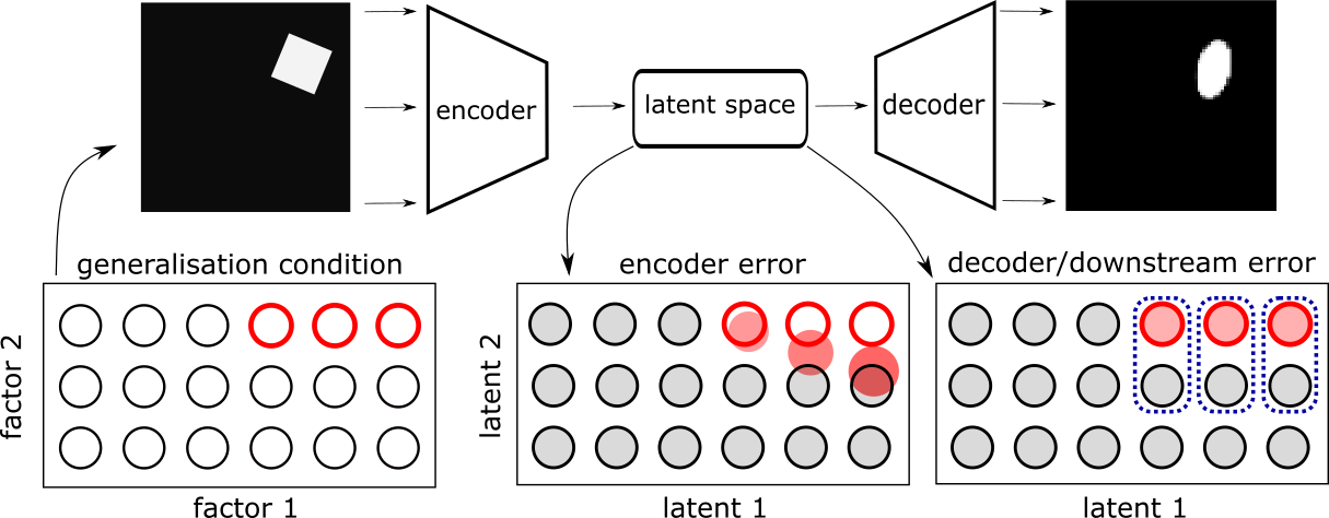
Figure 1: Possible problems for combinatorial generalisation. Left: visualisation of how a combinatorial generalisation condition can be defined for a dataset containing two generative factors. Black and red circles denote training and test examples, respectively. In the Middle and Right panels, the outline of each circle shows the target position of the representation in latent space, while a shaded circle shows the position at which the latent representation is projected by the encoder. Middle: first type of combinatorial generalisation error, encoder error. The encoder projects unseen inputs to different parts of the latent space than what was expected based on their generative factor values (shown as shaded circles falling outside their target outlines) Right: second type of combinatorial generalisation error, decoder error. Observed representations (shaded circles), are mapped to the correct position in latent space (circle outlines), but a decoder/downstream process mixes-up the black and red representations (blue dashed lines).

However, two recent studies have reported evidence that contradicts this hypothesis. Montero et al. (2020) considered datasets where inputs varied along several dimensions (generative factors) and divided generalisation conditions into different types. They found that VAEs with highly disentangled latent representations succeeded at the easiest generalisation conditions where only one combination of all generative factors was excluded (a condition they termed recombination-to-element), but failed at more challenging conditions, where all combinations of a subset of generative factors were excluded (termed recombination-to-range by Montero et al. (2020)). In another second study, Schott et al. (2021) tested 17 learning approaches, expanding the analysis to other paradigms, architectures and task structures. They observed that models showed moderate success at generalising on some artificial datasets, such as 3DShapes. However, their ability to generalise dropped significantly on more realistic datasets and in more challenging generalisation conditions.

These contradictory results could be down to a number of differences between studies that report successes and those that report failures. For example, there were qualitative differences in the datasets that were tested and how the test conditions were set up. This is indeed what Montero et al. (2020) conclude, writing that “it is not clear what exactly was excluded while training [previous models]”, suggesting that previously observed successes may have been on the simplest generalisation condition where only very few combinations were left out. But this still leaves open the question of why models that achieve high degree of disentanglement nevertheless fail at combinatorial generalisation under more challenging conditions.

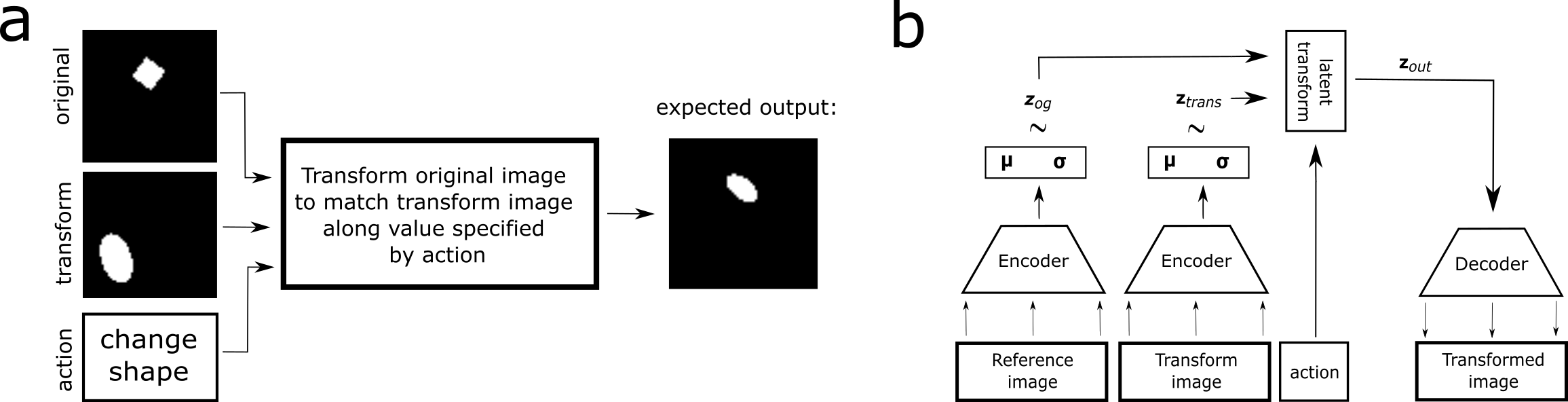
Figure 2: (a) Image composition task. An example of the composition task. In this case, the shape of the output must match the transform and the rest of the values must match the reference. (b) Model architecture. The model uses the same encoder to represent both images. Then a transform takes these latent representation and combines them to produce a transformed representation, which is used to reconstruct the output image. Reproduced from Montero et al. with permission from the authors.

We see two possible reasons why this could happen. One possibility is that models correctly infer the values of latent variables (Fig. 1, left) for novel combinations of generative factors, but the decoder fails to map these unseen latent values to the (output) image space – decoder error (Fig. 1, right). Some evidence supporting this hypothesis was observed by Watters et al. (2019), who looked at not only the output image reconstructions, but also at latent representations in a simple reconstruction task. Watters et al. (2019) observed that, in their task, models that have more disentangled latent representations do indeed map unseen combinations of generative factors to the correct values in the latent space. But they only tested a very simple dataset, involving only two generative factors. Montero et al. (2020) showed that models can sometimes succeed to generalise in simple settings where they can solve the combinatorial generalisation problem through interpolation, but struggle at more challenging settings where larger number of combinations are excluded from the training set.

Another possibility is that current models fail at harder forms of combinatorial generalisation (such as recombination-to-range) due to an encoding failure – encoder error. That is, the encoder fails to map these harder unseen combinations of generative factors to the correct values of variables in the latent space (Fig. 1, middle). If this were the case, then it reflects a more fundamental limitation of current models, showing that even though models can map observed combinations to correct values of latent representations, they do not understand how generative factors are combined. So when novel combinations are presented, models cannot infer the values of generative factors that led to the observed data.

In this work we first explore these issues by looking at the latent space of generative models. We start by replicating previous failures of image reconstruction for models that learn highly disentangled representations. We then show that failure to generalise in the output space is accompanied by failure to generalise in latent space across a broad range of datasets. We show that these results replicate for other architectures (such as a spatial broadcast decoder (Watters et al., 2019)) and other task settings (such as a supervised task set up to learn completely disentangled representations). Finally, by looking at the latent space, we discover that, in addition to the difficulty of the generalisation task, a crucial condition for failure of combinatorial generalisation is the way in which generative factors are combined.

2 The latent space of generative models

Even though there has been a concerted effort in the field to come up with models that have an increased degree of disentanglement, models still struggle to learn representations that are completely (or nearly completely) disentangled when they are learning standard tasks such as image reconstruction. This is problematic because it is difficult to test whether entangled models are projecting test data in the correct part of the latent space as there may be a nonlinear mapping between input space and latent space. Moreover, if these models fail to generalise, it could be argued that they do so because they fail to learn representations that are not “disentangled enough”. In this section we describe carefully chosen tasks and models that enable us to achieve latent representations that are highly disentangled. We also describe how we choose some challenging test conditions for combinatorial generalisation on some well known datasets.

2.1 Experimental Setup

2.1.1 Task

One of the main barriers to achieving disentanglement in standard unsupervised training is the non-identifiability of the models when using iid data (Hyvarinen & Morioka, 2016; Klindt et al., 2020). In short, this is because there are infinitely many linear combinations of the underlying generative factors that produce a valid basis on which they can be represented.

To solve this we used the composition task introduced in Montero et al. (2020). This task takes two images and a query vector as inputs. The goal of the task is to output an image that combines the two images based on an action in the query vector:

input $$=\mathbf{x_{og}},\;\mathbf{x_{trans}},\;\mathbf{q}$$

output $$=\mathbf{x_{out}}$$

where $\mathbf{x_{og}}$ and $\mathbf{x_{trans}}$ are the two input images, $\mathbf{x_{out}}$ is the output image, and $\mathbf{q}$ is the query vector. Following Montero et al., we used actions that involve replacing one of the properties (generative factors) of $\mathbf{x_{og}}$ with a property of $\mathbf{x_{trans}}$, based on the value of $\mathbf{q}$. This vector was a one-hot encoding of the generative factor that was required to be changed. We have shown an example of the composition task in Figure 2(a), where the goal of the model was to transform the original image, such that it replaces the given shape (square), but preserves all other attributes (position, scale and orientation).

By combining a semi-supervised component (the query vector plus image reconstruction) with sparse transitions (only one generative factor needed to be modified at a time), the composition task provided a strong inductive bias towards high levels of disentanglement, as has been shown in previous work that exploits these approaches (Locatello et al., 2020; Lin et al., 2020; Klindt et al., 2020).

2.1.2 Models

The model architecture used to solve the composition task is shown in Figure 2(b). It involves two encoders that map each image to a latent space. The latent vectors are then “composed” (see below), based on the query (action) vector. This composed vector is mapped from the latent space into the (output) image space using a decoder. Encoders and decoders for generative models match the ones used in past work (Higgins et al., 2017; Kim & Mnih, 2019) for both dSprites and 3DShapes datasets. For MPI3D we added another 2 more layers, which we found was necessary for models to learn the task. For the Circles dataset we used the encoder defined in Watters et al, along with the corresponding Spatial Broadcast Decoder architecture. Latent representations for the generative models are standard diagonal Gaussians with input dependent means and variances, to which we applied both the Variational and Wasserstein loss (Kingma & Welling, 2013; Tolstikhin et al., 2017).

We can define the composition operation that combines both latent representations as:

$$\mathbf{z_{out}=z_{og}\odot(1-c)+z_{trans}\odot c}$$

where $\mathbf{z_{out}}$, $\mathbf{z_{og}}$ and $\mathbf{z_{trans}}$ are the latent representations corresponding to the output, original, and transform images and $\odot$ is the element-wise product between vectors. The variable $\mathbf{c}$ is the interpolation vector of coefficients. We defined two ways of computing $\mathbf{c}$: (i) a learned interpolation function computed as $\sigma(W\cdot[\mathbf{z_{og};z_{trans};q}]+\mathbf{b})$ with parameters $W$ and $\mathbf{b}$ where $[.;.]$ represents the concatenation of vectors; and (ii) a fixed interpolation function $\mathbf{c}=\text{padded}(\mathbf{q})$ which just pads $\mathbf{q}$ with zeros to match the vector length of the latent representation (see Appendix A.2 for more details).

To facilitate our goal of testing combinatorial generalisation, we augmented the target output by requiring the model to reconstruct the input images as well. Thus the trained encoder and decoder form a valid standard autoencoder that we can test on the traditional unsupervised setting to see if the models generalise. An illustration of this model can be found in Figure 2.

2.1.3 Datasets

We tested our models on three standard datasets: dSprites (a sythesised dataset of 2D shapes procedurally generated from 5 independent generative factors (Matthey et al., 2017)), 3DShapes (another synthesised dataset consisting of 3D shapes procedurally generated from 6 ground truth generative factors (Burgess & Kim, 2018)) and MPI3D (a collection of four different datasets consisting of synthetic as well as real-world images procedurally generated from 7 generative factors (Gondal et al., 2019)). These are the most popular datasets used in the disentanglement literature that also provide ground truth generative factor values.

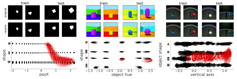
Figure 3: Generalisation in latent space Top: Typical examples of reconstructions for training and test images for models that learn highly disentangled representations. Bottom: Visualisation of the latent space of models trained on three datasets – dSprites (left), 3DShapes (middle) and MPI3D (right). Each panel shows the joint distribution of two latent variables that best predict the corresponding generative factors. In all cases, the red distributions indicate test data and the black ones indicate training data. Note that the latent values in this figure are not necessarily the same as the values of generative factors excluded. This is because every model ends up with a different internal representation based on its initialisation and sequence of training trials. However, in each case, we observed that these internal representations were highly structured when the model showed a high degree of disentanglement.

We tested combinatorial generalisation by systematically excluding combinations of values of generative factors from each dataset. Here we focus on the conditions described as recombination-to-range by Montero et al.. These are the most interesting conditions where, according to Montero et al., one would expect a model that learns disentangled representations to succeed at combinatorial generalisation, but tested models typically fail. Consider a dataset with, say, four generative factors [$g_{1}$, $g_{2}$, $g_{3}$, $g_{4}$] where all $g_{i}\in[0,1]$. The recombination-to-range condition creates a training/test split where all examples with combinations of a subset of generative factors are excluded from the training set and added to the test set. Thus, an example of a dataset that tests recombination-to-range may consist of a training set where all combinations where [$g_{1}>0.5$, $g_{2}>0.5$] have been excluded from the training set and added to the test set. Note that the model trained on such a datasets would come across a number of examples where [$g_{1}>0.5$] and also examples where [$g_{2}>0.5$], but never be trained on an example where both these conditions are true simultaneously. This method was used to create training / test sets for each of the datsets in the following manner:

• dSprites: All images such that [shape=square, posX$>0.5$] were excluded from the training set. Squares never appear on the right side of the image, but do appear on the left and other shapes (hearts, ellipsis) are observed on the right as well.

• 3DShapes: All images such that [shape=pill, object-hue=$>0.5$] were excluded from the training set. Thus, pills colored as any of the colors in the second half of the HSV spectrum did not appear in the training set. These colors (shades of blue, purple, etc) were observed on the other shapes, and the pill was observed with other colors such as red and orange.

• MPI3D: All images such that [shape=cylinder, vertical axis$>0.5$] were excluded from the training set. We also excluded all images where [shape=cone] or [shape=hexagonal] as these shapes are very similar to the pyramid and cylinder, respectively and make it hard to access reconstruction accuracy.

2.1.4 Measuring Disentanglement

We used the DCI metric from Eastwood & Williams (2018) to measure the degree of disentanglement (see Appendix A.5). This metric provides a set of regression weights between ground truth factors and latent variables. We selected the latent variable corresponding to each ground truth factor using a matching algorithm based on these weights. Crucially, for highly disentangled models any combination of generative factors will have a corresponding combination of latent variables of the same cardinality. This allows us to create visualisations of the latent representations analogous to the ones in Figure 1.

2.2 Results

We observed that most models trained on the composition task managed to achieve a reasonably high degree of disentanglement, and successfully reconstructed images in the training data (see Appendix B.2). Here we present results of typical models that achieved a very high degree of disentanglement (with alignment scores typically $>0.95$, see Appendix B for details). Figure 3 shows reconstructions as well latent space representations of three typical models trained on the dSprites, 3DShapes and MPI3D datasets, respectively.

Replicating results of Montero et al. (2020), we observed that models showed poor generalisation to unseen combinations for all three datasets (see reconstruction of test images in Figure 3). For dSprites, the models typically produced images with correct location, but made an error in the target shape (e.g., replacing the square with an ellipse). Similarly, with 3DShapes and MPI3D, models typically reconstructed shapes with the correct colour hue (3DShapes) or vertical location (MPI3D), but made an error in the shape of the target object (e.g., replacing the pill (3DShapes) or cylinder (MPI3D) with a sphere(3DShapes) or pyramid (MPI3D).

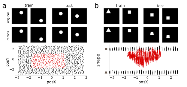
Figure 4: Latent space induced by SBD Visualisation of the latent space for models that use a Spatial Broadcast Decoder as described in Watters et al. Both visualisations correspond to a condition where combinations in the middle of the image are removed. (a) The result when this is done for the Circles dataset which uses only one shape and where the training set excludes all combinations [shape=circle, $0.35<$ posX $<0.65$, $0.35<$ posY $<0.65$] (b) The result for the a similar condition for the Simple dataset which uses two shapes and excludes all combinations [shape=square, $0.35<$ posX $<0.65$, $0.35<$ posY $<0.65$].

Next, we looked at the latent representations of each of these cases by selecting a latent variable that showed highest correlation with each generative factor as described in Section 2.1.4. Figure 3 plots the distributions of the value of each latent variable for every combination of values of the relevant generative factors. Visualising these probability distributions for the combination of generative factors seen during training (in black) confirmed that the models learned highly disentangled representations (note the low variance of the probability distributions for trained combinations, especially for dSprites and 3DShapes).

Crucially, we observed that the encoder failed to map the generative factors for the test combinations to the correct location in the latent space (red distributions). This was particularly true for dSprites and 3DShapes dataset: note how the mean of the probability distributions for the left out combinations ([shape=square, poxX$>0.5$] for dSprites and [shape=pill, object-hue=[blue, purple]]) are shifted to overlap the latent representations seen during training. The shifts in the mean of distributions were less acute for MPI3D, but we nevertheless observed an increase in the variability of test distributions and a consistent shift in means for values of generative factors that were far from the trained values.

In summary, we made three key observations in these experiments. First, models replicated the negative results reported previously: i.e., a degradation in reconstruction performance in the challenging combinatorial generalisation conditions. Second, by visualising the latent space, we observed that failures of generalisation coincided with poor latent representations, showing that failures of generalisation are not entirely due to decoder errors. Third, the failures in latent representations as well as output reconstructions showed that different generative factors have important qualitative differences, with models making larger errors in generating the correct shape for unseen combinations than in reproducing the position, scale or color (see Appendix B.2).

2.3 Exploring different decoder architectures

In the experiments above, we used the deconvolution network as the decoder, which is the standard decoder used in VAEs (Higgins et al., 2017). However, some studies have shown that replacing the deconvolution network with a different architecture helps the model learn representations that are more disentangled. One such architecture is the Spatial Broadcast Decoder (SBD from hereon) developed by Watters et al. (2019), who showed that such a decoder not only helped in learning representations that were highly disentangled, but also helped in solving the problem of combinatorial generalisation.

In our next set of experiments, we tested whether using the SBD succeeds at combinatorial generalisation in more challenging settings, akin to the ones we tested above. We first replicated the results for both conditions tested by Watters et al. (2019), using our composition task on the Circles dataset and replacing the deconvolution network with the SBD. Figure 4 (panel A) shows the results for the first condition, where the training set excluded images with circles presented in the middle of the canvas (see Appendix B.2 for results on the second condition). As we can see from this figure, the latent space learned by the model was indeed highly structured and, crucially, the model mapped the latent values for the left out combinations (red crosses) to the correct region of the latent space.

Next, we wanted to check how these results scaled when we made the generalisation test more challenging, excluding a combination of values for a range of variables (the recombination-to-range condition developed by Montero et al. (2020)). We can do this with the Circles dataset by adding a third generative factor and the simplest way of doing this is by letting the shape take one of several values, instead of being a circle for all examples.

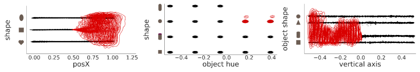
Figure 5: Supervised “latent space” Visualisation of the latent space for models trained to predict the correct generative factor values for each image. The visualizations correspond to the same test conditions as the ones presented in Figure 3: (a) dSprites, where all combinations where [shape=square, posX $>0.5$] were excluded from the training set (here, this corresponds to the middle latent value) (b) 3DShapes, where all combinations where [shape=pill, object-hue $>0.5$] were excluded (corresponding to the top latent value), and (c) MPI3D, where all combinations where [shape=cylinder, vertical-axis $>0.5$] were excluded (corresponding to the second from bottom value).

We tested this by constructing a new dataset called Simple. Like the Circles dataset, this dataset consisted of images that had a shape located at various (x and y) positions on the canvas. Unlike the Circles dataset, this shape could be either a triangle or a square (we chose these shapes as they are different enough for models to not confuse them by accident). We then tested the two conditions similar to the conditions tested by Watters et al. (2019), excluding all combinations where one of the shapes was presented in the middle (first condition) or the top-right (second condition) of the canvas.

The results for the first condition are shown in panel B of Figure 4 (see Appendix for results of the second condition). Like the results for the first set of experiments above, we have plotted the probability distribution of combinations of values of the the latent variables (here, shape and posX) for all values of the third latent variable (here, posY). Similar to our earlier results, we observed that even the model using the SBD failed to map the unseen (test) combinations to the correct position in the latent space (compare the mean and variability of the red distributions compared to the black ones). Correspondingly, we also observed that models failed to correctly reconstruct output images for the test conditions, even when they had no problem reconstructing these images for combination of generative factors seen during training (See Appendix B.2).

3 Replicating results on a different paradigm

We have shown that errors in generalisation occur in latent space as well in the reconstructions for generative models. To conclude this analysis we show that the problem does not lie in the generative nature of the task by testing the encoders on a supervised task. We used the same datasets and generalisation conditions as before.

3.1 Experimental setup

We trained models on a supervised task where the model was given a single image as the input and the target was to output the ground truth generative factor values. This ensures that the resulting latent representation will be completely disentangled, as the model must output each of the factor values separately. We used the mean squared error of the output and target vectors as a learning signal. All other parameters remain same as the composition task. We used the same architectures for the feed-forward models as the encoders in the corresponding datasets above.

We evaluated the models using the $R^{2}$ metric as used in Schott et al. (2021) to check whether the models had solved the task. We also use the same method to visualise the results as described above, plotting the joint probability distributions for the combination of generative factors along which the model was tested for generalisation. In this case, it is straightforward to do so as the relevant output dimensions shared the same index as the corresponding generative factor.

3.2 Results

The results for the three dataset are shown in Figure 5. We observed a very similar pattern for this supervised learning task as the unsupervised task above. For all three datasets, the probability distributions of latent values for the left out combinations (in red) showed a much higher variance and means that were shifted towards combinations of latent values that had been experienced during training. Thus, even when the encoders were trained to recognise perfectly disentangled generative factors, they failed to generalise their mapping to combinations that were not experienced during training.

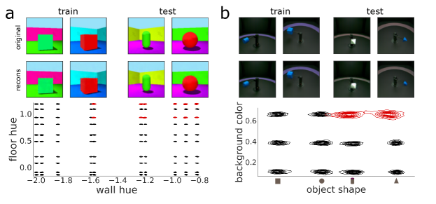
Figure 6: Latent space for conditions where models succeed Visualisation of the latent space for models trained on conditions in which they succeed at generalisation. The figure follows the same conventions as in Figure 3. (a) Results for 3DShapes when removing floor and wall color combinations. (b) Visualisation for the MPI3D dataset for combinations where the salmon background has not been seen with the cylinder shape.

4 Explaining contradictory findings

How can we reconcile the failures of generalisation observed above with with past studies that showed successful combinatorial generalisation on some datasets and conditions? One response is that the generalisation conditions we test are more challenging than the ones tested in previous studies because they exclude more data from the training set. However, it is also possible that the success of combinatorial generalisation is not only determined by how many combinations are excluded from the test condition, but also by which combination of generative factors are tested.

All failures observed above were for cases where the generative factor ‘shape’ is combined with another generative factor (position / color). We obtained qualitatively similar results when we tested shape in combination of other generative factors, such as orientation. It is possible that this was because shape combines with other factors in a qualitatively different manner than, say, the floor hue combines with the wall hue in 3DShapes. In order to completely disentangle shape from position / color / orientation, the model must come up with a representation of shape that is invariant to a change in these generative factors. And it must do so by learning from training examples where shape and orientation interact – that is, the observed image is obtained via a composition of the two generative factors affecting the same part of the image.

But not all combinatorial generalisation problems face this problem of working out how generative factors combine to determine the same part of the observed image. In some cases, an image may be determined by a combination of generative factors, but each factor governs a different part of the image, such as the generative factors [floor-hue, wall-hue] in 3DShapes. In such cases, learning a representation of one factor that remains invariant to the other factor is trivial and the model may succeed at combinatorial generalisation, even though the same amount of data is excluded from the training set. To test this hypothesis, we carried out a set of experiments where the model had to solve the problem of combinatorial generalisation, but the combinations that were excluded did not interact in the training examples. We can do this for both the 3DShapes dataset as well as the MPI3D dataset, as both datasets involve images where the canvas contains several disjoint elements. So, we repeated the unsupervised learning experiments above, where models had to learn the composition task, but instead of excluding combinations where the generative factors interacted with each other, we excluded the following combinations from the training set:

• 3DShapes: Exclude all combinations such that [floor-hue $<0.25$, wall hue $>0.75$]. That is, none of the training images had the combination of floors with a “warm” hue and walls with a “cold” hue.

• MPI3D: Exclude all combinations such that [shape={cylinder,sphere}, background color=salmon]. Note, even though the excluded combination here involves shape, the combination of generative factors excluded do not interact in an image (i.e. determine different parts of the image).

4.1 Results

Unsurprisingly, we again observed that models learned highly disentangled representations for this task. More interestingly, we also observed that models now succeeded at the combinatorial generalisation task. Figure 6 shows some typical reconstructions for training as well as test images. These reconstructions successfully reproduce the unseen combination of floor hues and wall hues for the 3DShapes dataset and the combination of shape and background arc color for the MPI3D dataset. This figure also shows the joint probability distribution for trained as well as novel combination of latent values. Unlike the results observed above ( Figure 3), we now see that the latent distributions for unseen combinations (in red) have means that fall in the expected location and a much smaller variance..

5 Discussion

Our world is inherently compositional – it can be decomposed into simpler parts and relationships between these parts. The idea behind learning disentangled representations is to recover this underlying compositional structure of the world from perceptual inputs. Unsupervised learning models, such as VAEs, aim to do this by separating out the factors that remain invariant under transformations of other factors (Higgins et al., 2018a). It is therefore tempting to conclude that models that manage to show a high degree of disentanglement on the training set also capture the compositional structure of the world. If they did, they should be able to generalise to settings that present novel combination of the factors of variation. However, in our experiments, we observed that models that learned highly disentangled representations nevertheless failed at combinatorial generalisation, not only in the reconstruction space, but also in the latent space.

Our interpretation of these results is that models manage to achieve a high degree of disentanglement by discovering factors that remain invariant over training examples and simply associating perceptual inputs with these factors. However, to capture the compositional structure of the world, models must additionally understand how factors interact to cause the perceptual input – that is, develop a good causal model of the world. We think the failure of models to form such a causal model is the reason behind why models succeeded at problems of combinatorial generalisation that do not involve an interaction between the left-out factors (Figure 6), but consistently failed at problems where these factors interacted (Figure 3). When generative factors do not interact, the model does not need to learn how the factors combine to determine the same part of the output space. Instead, it can simply map the value of each generative factor to a different location. It appears to solve combinatorial generalisation, but it does not understand how generative factors combine.

In an analogous way, we would suggest that the past successes of generalising in the leave-one-out setting (Montero et al, 2021) are an example of models only appearing to solve combinatorial generalisation. In this setting, it is possible to generalise either through combinatorial generalisation or simple interpolation given the untrained test items are so similar to trained items. We suggest that models are succeeding by the latter method. But when models are forced to combine familiar but previously unpaired features (because the factors interact) and are prevented from solving generalisation through interpolation (by removing more combinations) both encoders and decoders fail. Thus, in addition to aiming for models that show a higher degree of disentanglement, research should focus on models that can solve the problem of combinatorial generalisation. This will lead to models that have a better understanding of the compositional structure of our world (Hummel, 2000).

6 Acknowledgments

The authors would like to thank the members of the Mind & Machine Learning Group and Neural and Machine Learning Lab for useful comments throughout the different stages of this research. This research was supported by a ERC Advanced Grant, Generalization in Mind and Machine #741134.

Appendix A Experimental setup

A.1 Task

Here we describe the image composition task in more detail. This task was created by Montero et al. (2020) to check whether a different task than simple image reconstruction helps the model to learn more disentangled representations and as a consequence show combinatorial generalisation. At a high level the task is a manipulation task, where models must learn to extract the relevant factors $g_{i}$ from two images, $X_{og}$ and $X_{trans}$, and combine them based on a given ‘action’:

input $$=X_{og},\;X_{trans},\;\mathbf{q}$$

output $$=X_{out}$$

where $X_{out}$ is the output image and $\mathbf{q}$ is the query vector, that encodes the action. Following Montero et al., we use actions that involve replacing one of the properties (generative factors) of $X_{og}$ with a property of $X_{trans}$. The query vector uses a one-hot encoding of the generative factor that must be changed. See Figure 2 for an example of this task.

A critical aspect of this task is that it requires the change to be only one generative factor for each trial. Restricting the manipulation to a single generative factor encourages sparseness of representations and provides a strong inductive bias for the model to learn disentangled representations. Previous research has shown that sparse transitions following natural image statistics provide a strong inductive bias towards disentanglement (see, for example, Klindt et al. (2020)). This is because breaking the i.i.d. assumption, present in most datasets, allows for the identification of the underlying factors (see Klindt et al. (2020) for details and Hyvarinen & Morioka (2016) for a similar argument for selecting independent components from data).

A second inductive bias towards disentanglement is provided by the nature of the composition task. In contrast to a reconstruction task, that doesn’t provide any supervision signal, and a classification task, which provides a strong supervision signal, the composition task uses a query vector to provide a weak supervision signal. Two studies have shown that a weak supervision signal can provide a strong inductive bias for generalisation. Locatello et al. (2020) showed that a few labeled examples were enough to significantly improve the disentanglement in generative models. In the second study, Lin et al. (2020) developed a task with a weak supervision signal, where the target was to identify the factor that had changed between two images. They used this task to train a GAN and show it leads to more disentangled representations. The query vector in the composition task constitutes a similar weak supervision signal, but provided as an input instead of as a target.

A.1.1 Procedure

When training models, we sampled each combination in an online fashion. The procedure works as follows:

1. Sample an image $X_{og}$ and with generative factors given by the vector $\mathbf{g_{og}}$ from the dataset.

2. Sample an action, $a$, that indexes the set of all generative factors, $\{g_{1},\dots,g_{n}\}$.

3. Sample a second image $X_{trans}$ such that $\mathbf{g_{trans}}[a]$, the $a$th generative factor of $X_{trans}$ does not match $\mathbf{g_{og}}[a]$, the $a$th generative factor of $X_{og}$.

4. Compute $\mathbf{g_{out}}$ by replacing $\mathbf{g_{og}}[a]$ with $\mathbf{g_{trans}}[a]$ and get and it’s associated image $X_{out}$.

All sampling is done uniformly and we allow sampling of categorical variables such as shape.

A.2 Models

A.2.1 Composition operation

We use the general architecture described in Figure 2(b) to define a model that solves the composition task. As mentioned in the main text this requires the definition of the composition operation, $f(\cdot)$ in latent space. In general, such operation can be defined as:

$$\mathbf{z_{out}}\triangleq f(\mathbf{z_{og}},\mathbf{z_{trans}},\mathbf{q})$$

where $\mathbf{z_{out}}$, $\mathbf{z_{og}}$ and $\mathbf{z_{trans}}$ are the latent representations corresponding to the output, original, and transformation images. and $\mathbf{q}$ is the one-hot vector encoding the action to be performed.

We defined 3 different versions of this operation:

$$f_{mlp}(\mathbf{z_{og}},\mathbf{z_{trans}},\mathbf{q}) =\mathbf{W}_{out}\cdot\text{ReLU}(\mathbf{W}[\mathbf{z_{og}};\mathbf{z_{trans}};\mathbf{q}]+\mathbf{b})$$ (1)

$$f_{lin}(\mathbf{z_{og}},\mathbf{z_{trans}},\mathbf{q}) =W_{out}\cdot[\mathbf{z_{og}};\mathbf{z_{trans}};\mathbf{q}]$$ (2)

$$f_{interp}(\mathbf{z_{og}},\mathbf{z_{trans}},\mathbf{q}) =\mathbf{z_{og}}\odot(1-\mathbf{c})+\mathbf{z_{trans}}\odot\mathbf{c}$$ (3)

where $[.;.]$ represents the concatenation of vectors, $\mathbf{c}$ is the interpolation vector of coefficients. We define $\mathbf{c}$ in two ways for equation 3 as described in the main text:

$$\mathbf{c_{learn}} =\sigma(\mathbf{W}\cdot[\mathbf{z_{og}};\mathbf{z_{trans}};\mathbf{q}]+\mathbf{b})$$ (4)

$$\mathbf{c_{action}} =\text{pad}(\mathbf{q},\text{length}(\mathbf{z})-\text{length}(\mathbf{q}))$$ (5)

where the first option has learnable parameters $W$ and $\mathbf{b}$. The second just pads the query vector, $\mathbf{q}$, with zeros to match the vector length of the latent representation.

Preliminary tests showed that using (1) or (2) as composition operations lead to poor disentanglement. Thus we only tested the two variants of (3) in the rest of the experiments. For some datasets such as dSprites, (5) worked better. For 3DShapes on the other hand, (4) gave better results.

A.2.2 Encoder and Decoder architectures

For the rest of the architectures (encoders and decoders) we use the same parameters across datasets for each condition. For dSprites and 3DShapes, we use a similar architecture as in Kim & Mnih (2019) but increase the number of channels in the early convolutions. MPI3D required us to increase these values again in order to achieve good reconstructions. For Circles and Simple we use the architecture proposed in Watters et al. (2019) but slightly increase the channel size in the decoder to avoid a performance overhead related to PyTorch’s implementation. See Table 1 for details.

Table 1: Architecture parameters

dSprites & 3DShapes		MPI3D		Circles & Simple
Encoder	Decoder	Encoder	Decoder	Encoder	Decoder
Conv(32, 4, 2)	Transpose	Conv(64, 4, 2)	Transpose	Conv(64, 4, 2)	SBD(64, 64)
Conv(32, 4, 2)	of encoder	Conv(64, 4, 2)	of encoder	Conv(64, 4, 2)	Conv(64, 5, 1)
Conv(64, 4, 2)		Conv(128, 4, 2)		Conv(64, 4, 2)	Conv(64, 5, 1)
Conv(64, 4, 2)		Conv(128, 4, 2)		Conv(64, 4, 2)	Conv(64, 5, 1)
Conv(128, 4, 2)		Conv(256, 4, 2)		Linear(256)	Conv(64, 5, 1)
Linear(256)		Linear(256)		Linear(20)
Linear(20)		Linear(20)

All layers where followed by ReLU activation functions except for the last one. The latent layers used were 10-dimensional, parameterized diagonal Gaussians in all cases. For both the Conv and DeConv layer the parameters indicate number of channels, size of convolution filter and the stride. “Same” padding was used throughout. For completion, we note that the architectures for the supervised task were the same ones as the corresponding encoder.

A.3 Datasets

Throughout the article we use standard datasets used to test disentangled models in the literature. These are: dSprites, 3DShapes, MPI3D and Circels. Below we describe each of the generative factors they contain. We’ve focused on datasets that have been specifically designed for this purpose and thus contain explicit values of the generative factors. This is necessary in order to compute the level of disentanglement with most metrics, including the DCI metric.

• dSprites: Introduced in Higgins, (2017) to test the original $\beta$-VAE approach to disentanglement. It contains the following generative factors: [shape, scale, orientation, position X, position Y]. Orientation here refers to the rotation of the shape along it’s center of mass. This is as opposed to the meaning in 3DShapes (see below). The GitHub repository for dSprites can be found at: https://github.com/deepmind/dsprites-dataset.

• 3DShapes: Introduced in Kim (2019), to study the FactorVAE penalty. It contains the 6 generative factors: [floor hue, wall hue, object hue, scale, shape, orientation]. Colors are defined in the HSV format, and the values correspond to the hue component. Here orientation defines the angle of point-of-view for the scene. The objects themselves do not rotate. This dataset can be found at: https://github.com/deepmind/3d-shapes.

• MPI3D: This dataset was proposed in Gondal et al, (2019) as part of the the NEURIPS Disentanglement Challenge. It contains seven generative factors: [object color, object shape, object size, camera height, background color, horizontal axis, vertical axis]. We note that vertical axis and horizontal axis have complex non-linear dependencies between them in the rendered image. The names can also be misleading as horizontal axis controls the height of the arm while vertical axis controls the rotation in the direction perpendicular to the horizontal axis. The GitHub repository for this dataset can be found at: https://github.com/rr-learning/disentanglement_dataset.

• Circles: Introduced to test the capabilities of the Spatial Broadcast Decoder models in Watters et al, (2019). It contains only two factors: [position x, position y], the model being required to only render circles at the relevant position. There is no published dataset in this case, though the authors mention that they generated this dataset using the Spriteworld library, which is a library designed to generate simple datasets for reinforcement learning. We adapted the library to generate still images similar to those found in Watters et al. (2019).

• Simple: We modified the Circles dataset to create the Simple Sprites dataset in order to test the effect of introducing an additional shape when testing the combinatorial generalisation capabilities of the Spatial Broadcast decoder. In addition to the two position factors in the Circles dataset, we added a shape factor that could take one of two values [shape={triangle,square}]. We chose these shapes so that they are sufficiently different from each other. To generate the dataset we use the same library that we use to replicate the Circles dataset above.

A.3.1 Combinatorial generalisation test conditions

For each dataset we tested one success condition and one failure condition. These all constitute recombination-to-range conditions as definde in (Montero et al., 2020) but we refer to them as combinatorial generalisation conditions . The failure conditions were defined as follows

• dSprites: All images such that [shape=square, posX$>0.5$] were excluded from the training set. Squares never appear on the right side of the image, but do appear on the left and other shapes (hearts, ellipsis) are observed on the right as well.

• 3DShapes: All images such that [shape=pill, object-hue=$>0.5$] were excluded from the training set. Thus, pills colored as any of the colors in the second half of the HSV spectrum did not appear in the training set. These colors (shades of blue, purple, etc) were observed on the other shapes, and the pill was observed with other colors such as red and orange. Additionally we removed every other color from the dataset. This helped us clearly discretize the generative factors and latent representations, allowing us to clearly observe the performance of the models in the latent space.

• MPI3D: All images such that [shape=cylinder, vertical axis$>0.5$] were excluded from the training set. We also excluded all images where [shape=cone] or [shape=hexagonal] as these shapes are very similar to the pyramid and cylinder, respectively and make it hard to access reconstruction accuracy. Furthermore, only images with [horizontal axis=0] were included as rotation of both horizontal and vertical axis make it hard to find completely unseen combinations due to how much rotation of the objects is involved.

• Circles: All images such that [posX $0.5$,posY$>0.5$] were excluded from the training set. Models have not seen circles in the top right corner.

• Simple: All images such that [$0.35<$ posX $0.65$,$0.35$ posY$>0.65$,shape=triangle] were excluded from the training set. Similar to the previous condition, but now the unseen triangles lie in a patch in the middle of the screen. Squares were presented on all positions, similar to dSprites.

And the success ones as:

• 3DShapes: These test images presented a novel combination of generative factors, here [floor hue $<0.25$, wall hue $>0.75$] – that is, the model has seen all wall hues and floor hues in the range $[0,1]$, but it has never seen a combination a floor with a hue $<0.25$ with a wall of a hue $>0.75$. In this case no discretization was necessary, as the task is easy enough that the model obtained good disentanglement and the visualisations were easy to understand.

• MPI3D: All images such that [shape={cylinder,sphere}, background color=salmon] were excluded from the training set. We also excluded all images where [shape=cone] or [shape=hexagonal] as these shapes are very similar to the pyramid and cylinder, respectively and make it hard to access reconstruction accuracy. Furthermore, only images with [horizontal axis=0] were included as rotation of both horizontal violate our independence assumption. Models can appear over the background strip very often.

• Circles: All images such that [$0.35<$ posX $0.65$,$0.35$ posY$>0.65$] were excluded from the training set. Models have not seen circles in a patch located in the middle of the image.

A.4 Training

To penalise the models we use the standard VAE objective (Kingma & Welling, 2013) and the Wasserstein loss (WAE, Tolstikhin et al. (2017)). In the case of the MPI3D dataset, WAEs were the only one that could successfully converge for the unsupervised setting, which we use as a sanity check. This is likely because the VAE objective forces the distribution of the latent representation for each input to match the prior. On the other hand WAEs only require the marginal posterior over all inputs to match the prior. The result is a latent representation that is more flexible, which seems to be required in this more complex dataset. As a consequence, we do not test VAE models on the MPI3D dataset for the composition task.

We trained the models to convergence, which in all cases occurred within 100 epochs. Batch sizes were kept at 64 and learning rates at $1e-4$ as in previous work for dSprites, 3DShapes and MPI3D. For the Circles dataset we used a batch size of 16 and a learning rate of $3e-4$ as in Watters et al.. We used the Adam optimizer with the default PyTorch values for all remaining parameters (Kingma & Ba, 2017).

A.5 Measuring disentanglement

We measured disentanglement using the DCI metric of Eastwood & Williams (2018). DCI defines three different metrics: disentanglement, completeness and informativeness. For our purposes, we are only interested in the first, but they are all computed in a similar way. Disentanglement here is defined as the degree to which a latent variable represents at most one and only one generative factor.

Let $v_{j}$ be the ground truth values for each factor $g_{j}$. Assuming a trained model, the metric works as follows:

1. Compute the latent representation $z_{n}$ = $\text{encode}(x_{n})$ for all images $x_{n}$ in the dataset.

2. For each factor $g_{j}$ solve a regression problem with the $z_{n}$’s as covariates.

3. Construct a matrix $C$, where each index, $c_{ij}$, is the absolute value of the regression coefficient between the latent variable $i$ and generative factor $j$.

4. $C$ is then used to quantify the deviation of the latent representation from the ideal one.

The authors propose using Lasso regression or Random Forests (they provide a method to determine the coefficient for the latter). In this work we use Lasso with their proposed hyper-parameters. To compute the disentanglement score, the coefficients in $C$ are treated as a distributions, one for each column (latent), from which the entropy is computed:

$$H(P_{i})=-\sum^{J}_{j=0}P_{ij}\log_{J}P_{ij}$$

where $P_{ij}=C_{ij}/\sum_{k=0}^{J}C_{ik}$, where $J$ denotes the number of rows in $C$. The score for one variable is computed as:

$$d_{i}=1-H(P_{i})$$

The $d_{i}$’s are then be averaged to obtain the final, overall disentanglement score:

$$D =\sum_{i}\rho_{i}\cdot d_{i}$$

$$\rho_{i} =\frac{\sum_{j=0}^{J}C_{i,j}}{\sum_{l,j}C_{l,j}}$$

where the $\rho_{i}$ are computed so as to account for dead units in the representation. We refer to $D$ as the disentanglement score throughout the main text, in line with most research on the topic.

DCI is interesting for a couple of reasons. First, it computes it’s scores based on the ability to predict values from the latent representations. Additionally, the coefficients $C$ can be visualized using Hinton matrices, which means we can use it for both quantitative measurements and for visual inspection of the trained models, as we see below. An ideal model in this framework will produce a matrix $C$ that is diagonal, up to some permutation of the latent variables and disregarding any extra dimensions used in the latent representation (see Figure 7 for an example). This fits well with intuitions regarding disentanglement and with the definition proposed in Higgins et al. (2018a).

Given these coefficients, it is easy to assign latents to the corresponding generative factor. To avoid assigning a latent to two factors, we used the Munkres algorithm (Munkres, 1957) as in Hyvarinen & Morioka (2016). For a highly disentangled model we can use this assignment to visualize pairs of latent variables in a 2D plot.

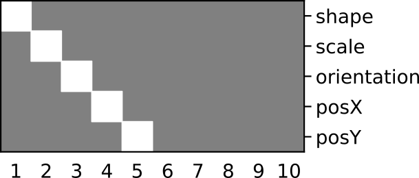
Figure 7: Ideal disentanglement Example of ideal disentanglement computed with the DCI metric for the dSprites dataset.

A.6 Implementation

All the models and tasks where implemented in PyTorch (version $\geq$ 3.8, Paszke et al. (2019)) and Numpy (Harris et al., 2020). The experiments where performed with the aid of the Ignite and Sacred frameworks (Fomin et al., 2020; Klaus Greff et al., 2017). Visualizations were created using Matplotlib (Hunter, 2007) and Seaborn (Waskom, 2021). Code required to reproduce the results will be made public after review process is complete .

Appendix B Results

Below we provide Model scores (that were used to measure success at reconstruction as well as degree of disentanglement), some example reconstructions for each type of model and Hinton matrices that are useful to visualising the degree of disentanglement. We also provide visualisations of the latent space (akin to the ones presented in the main text). In each case, we present examples of two types of training objective (VAE & WAE – see Section A.4) and two types of interpolation (fixed and learned – see Equations 5 and 4) – making a total of four models for each condition (except for the MPI3D dataset where only models trained with the WAE objective succeeded in learning the task).

B.1 Model scores

Table 2: Scores for dSprites failure condition The scores for the condition [shape=square,posX>0.5]. Reconstruction loss for VAEs are computed with pixel-wise binary cross-entropy (Bernoulli loss). For the WAE it is the pixel-wise mean squared error.

	Train loss	Test loss	Disentanglement
Model
VAE + learned interp	8.353618	183.369238	0.881088
VAE + fixed interp	7.524311	366.997949	0.999999
WAE + learned interp	2.310111	44.854529	0.917322
WAE + fixed interp	2.038967	45.108577	0.983566

Table 3: Scores for 3DShapes failure condition The scores for the condition [shape=pill,object hue={blue, purple}]. Reconstruction loss for VAEs are computed with pixel-wise binary cross-entropy (Bernoulli loss). For the WAE it is the pixel-wise mean squared error.

	Train loss	Test loss	Disentanglement
Model
VAE + learned interp	3459.323259	5050.596667	0.980030
VAE + fixed interp	3460.841481	5517.578000	0.960200
WAE + learned interp	5.905513	214.398937	0.999999
WAE + fixed interp	7.470970	224.247479	0.973512

Table 4: Scores for 3DShapes success condition The scores for the condition [wall hue={red, orange},floor hue{purple, magenta}]. Reconstruction loss for VAEs are computed with pixel-wise binary cross-entropy (Bernoulli loss). For the WAE it is the pixel-wise mean squared error.

	Train loss	Test loss	Disentanglement
Model
VAE + learned interp	3467.451818	3498.955556	0.975767
VAE + fixed interp	3471.045758	3510.643056	0.893841
WAE + learned interp	5.079037	6.359890	0.972172
WAE + fixed interp	5.932047	32.906424	0.948327

Table 5: Scores for MPI3D failure condition The scores for the condition [object shape=cylinder,vertical axis >0.5]. Reconstruction loss for VAEs are computed with pixel-wise binary cross-entropy (Bernoulli loss). For the WAE it is the pixel-wise mean squared error.

	Train loss	Test loss	Disentanglement
Model
WAE + learned interp	2.114849	4.598420	0.675261
WAE + fixed interp	1.586387	5.227437	0.976362

Table 6: Scores for MPI3D failure condition The scores for the condition [shape={cylinder,sphere}, background color=salmon]. Reconstruction loss for VAEs are computed with pixel-wise binary cross-entropy (Bernoulli loss). For the WAE it is the pixel-wise mean squared error.

	Train loss	Test loss	Disentanglement
Model
WAE + learned interp	2.014464	2.271657	0.702668
WAE + fixed interp	1.694517	2.517065	0.966975

Table 7: Scores for the Circles dataset The scores for the two conditions in the score dataset. The “corner” condition excludes instances with [posX>0.5, posY>0.75]. The condition “midpos” excludes those with [0.35<posX<0.65,0.35<posY<0.65].

	Condition	Train loss	Test loss	Disentanglement
Model
VAE + fixed interp	corner	113.977726	4313.172778	0.843828
VAE + fixed interp	midpos	115.894145	157.793549	0.781331

Table 8: Scores for the Simple dataset The scores for the two conditions in the score dataset. The “corner” condition excludes instances with [posX>0.5, posY>0.75,shape=triangle]. The condition “midpos” excludes those with [0.35<posX<0.65,0.35<posY<0.65,shape=triangle].

	Condition	Train loss	Test loss	Disentanglement
Model
VAE + fixed interp	corner	129.493923	523.572257	0.901404
VAE + fixed interp	midpos	129.802943	267.656094	0.936586

B.2 Reconstructions

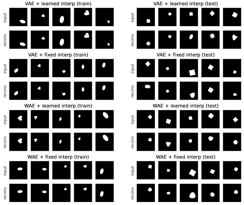
Figure 8: Failures of combinatorial generalisation on dSprites Some example reconstructions for the dSprites dataset for four models: (i) a VAE using learned interpolation (see Equations 4), (ii) a VAE using a fixed interpolation (see Equation 5), (iii) a WAE using a learned interpolation, and (iv) a WAE using a fixed interpolation. In each case, the five figures on the left show input (first row) and reconstruction (second row) for five training images. The five figures on the right show input and reconstructions for test images. These test images presented a novel combination of generative factors, here [shape=square, posX $>0.5$] – that is, the model has seen all shapes on both the left and right hand side of the canvas, except squares, which have only been seen on the left hand side (posX $<0.5$). All models learn representations that are highly disentangled. While reconstructions on the training dataset are really accurate - it is clear to see that the models struggle to reconstruct the test images, where a square is presented on the right hand side of the canvas.

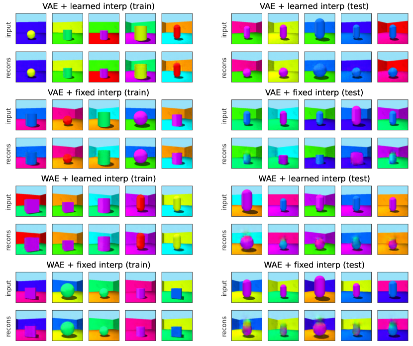
Figure 9: Failures of combinatorial generalisation on 3DShapesSome example reconstructions for the 3DShapes dataset for four models: (i) a VAE using learned interpolation (see Equations 4), (ii) a VAE using a fixed interpolation (see Equation 5), (iii) a WAE using a learned interpolation, and (iv) a WAE using a fixed interpolation. All models learn representations that are highly disentangled. In each case, the five figures on the left show input (first row) and reconstruction (second row) for five training images. The five figures on the right show input and reconstructions for test images. These test images presented a novel combination of generative factors, here [shape=pill, object hue $>0.5$] – that is, the model has seen all the combinations of shapes and hues for the object in the middle of the image, except for the ‘pill’ shape, which has only been seen in “warmer” colors (object hue $<0.5$). We observed that while reconstructions on the training dataset were really accurate - it is clear to see that the models struggled to reconstruct the test images, where the object was a ‘pill’ shape with a “cooler” color.

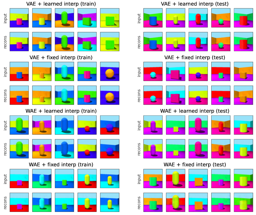
Figure 10: Success in combinatorial generalisation on 3DShapes Some example reconstructions for the 3DShapes dataset for four models: (i) a VAE using learned interpolation (see Equations 4), (ii) a VAE using a fixed interpolation (see Equation 5), (iii) a WAE using a learned interpolation, and (iv) a WAE using a fixed interpolation. All models learn representations that are highly disentangled. In each case, the five figures on the left show input (first row) and reconstruction (second row) for five training images. The five figures on the right show input and reconstructions for test images. These test images presented a novel combination of generative factors, here [floor hue $<0.25$, wall hue $>0.75$] – that is, the model has seen all wall hues and floor hues in the range $[0,1]$, but it has never seen a combination a floor with a hue $<0.25$ with a wall of a hue $>0.75$. We observed that, in this case, the model succeeded at combinatorial generalisation, reconstructing the images equally well on the training and test sets (compare with Figure 9).

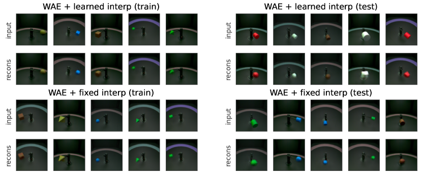
Figure 11: Failures of combinatorial generalisation on MPI3D Some example reconstructions for the MPI3D dataset for two models: (i) a WAE using learned interpolation (see Equations 4), (ii) a WAE using a fixed interpolation (see Equation 5). Both models learn representations that are highly disentangled. In each case, the five figures on the left show input (first row) and reconstruction (second row) for five training images. The five figures on the right show input and reconstructions for test images. These test images presented a novel combination of generative factors, here [shape=cylinder, vertical axis $>0.5$] – that is, the model has seen all the combinations of shapes (of the object at the end of a rod) and positions on the vertical axis, except for the cylinder, which has only been seen at vertical axis positions $<0.5$). We observed that while reconstructions on the training dataset were really accurate - both models struggled to reconstruct the test images with the left out combination of shape and position, frequently replacing the shape of the object.

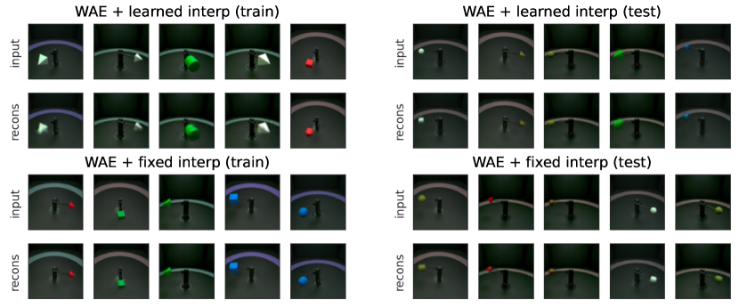
Figure 12: Success in combinatorial generalisation on MPI3D Some example reconstructions for the MPI3D dataset for two models: (i) a WAE using learned interpolation (see Equations 4), (ii) a WAE using a fixed interpolation (see Equation 5). Both models learn representations that are highly disentangled. In each case, the five figures on the left show input (first row) and reconstruction (second row) for five training images. The five figures on the right show input and reconstructions for test images. These test images presented a novel combination of generative factors, here [shape={cylinder,sphere}, background color=salmon]. We observed that, in this case, the model managed to successfully perform the task of combinatorial generalisation, reproducing the training as well as the test images with really good accuracy (compare with 11).

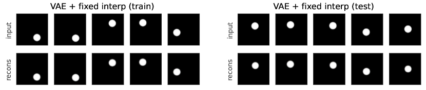
Figure 13: Success in combinatorial generalisation on Circles dataset Some example reconstructions for the Circles dataset. The model learns representations that are highly disentangled using fixed interpolation (see Equation 5). The five figures on the left show input (first row) and reconstruction (second row) for five training images. The five figures on the right show input and reconstructions for test images. These test images presented a novel combination of generative factors, here [$0.35<$ posX $<0.65$, $0.35<$ posY $<0.65$] – that is, the model has seen circles in all x-positions, as well as all y-positions, but never for a combination of x & y positions that fall in a central patch. We observed that the models managed to successfully perform the task of combinatorial generalisation, reproducing the circle in all positions of the canvas.

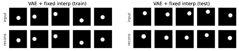
Figure 14: Failure in combinatorial generalisation on Circles dataset Some example reconstructions for the Circles dataset. The model learns representations that are highly disentangled using fixed interpolation (see Equation 5). The five figures on the left show input (first row) and reconstruction (second row) for five training images. The five figures on the right show input and reconstructions for test images. These test images presented a novel combination of generative factors, here [posX $>0.5$, posY $>0.5$] – that is, the model has seen circles in all x-positions, as well as all y-positions, but never for a combination of x & y positions that fall in a top right corner. We observed that the models failed in this condition in line with results in Watters et al. (2019)

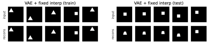
Figure 15: Failures of combinatorial generalisation on Simple dataset for the middle patch condition Some example reconstructions for the Simple dataset for two models: The model learns representations that are highly disentangled using fixed interpolation (see Equation 5). The five figures on the left show input (first row) and reconstruction (second row) for five training images. The five figures on the right show input and reconstructions for test images. These test images presented a novel combination of generative factors, here [$0.35<$ posX $<0.65$, $0.35<$ posY $<0.65$,shape=triangle] – that is, the model has seen triangles in all x-positions, as well as all y-positions, but never for a combination of x & y positions that fall in a central patch. It has seen squares in a central location. We observed that the models failed to proprely generalise in this condition, as opposed to the corresponding condition in the circles dataset (see Figure 13

B.3 Disentanglement

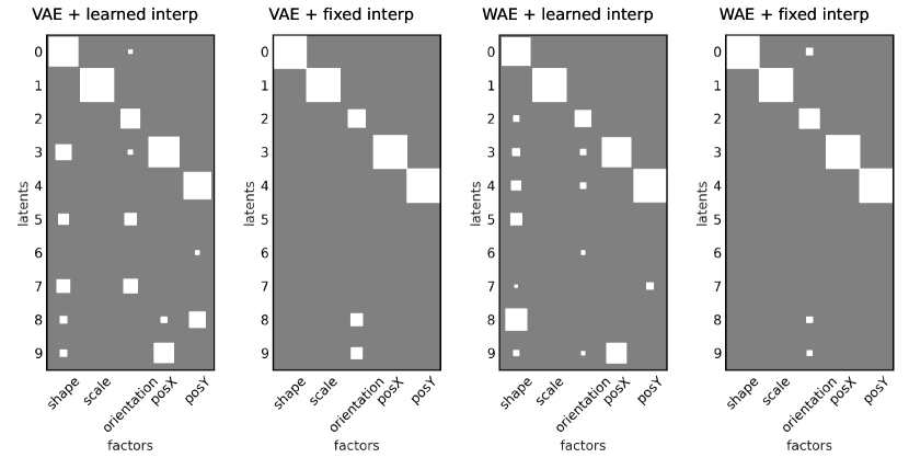
Figure 16: Visualising disentanglement for dSprites dataset Following Eastwood & Williams (2018), we used Hinton matrices to visualise the extent of disentanglement. Each panel shows the matrix $C$ (see Section A.5) of regression coefficients between latent variables and generative factors. A disentangled model should have high coefficients for each pair of generative factors and latent variable but low coefficients everywhere else – i.e. the matrix should be sparse (see ideal Hinton matrix in Figure 7). Here we can see that all models learning the composition task show highly sparse matrices and models using fixed interpolation (Equation 5) achieve particularly high disentanglement.

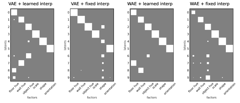
Figure 17: Visualising disentanglement for 3DShapes dataset, failure condition Following Eastwood & Williams (2018), we used Hinton matrices to visualise the extent of disentanglement. Each panel shows the matrix $C$ (see Section A.5) of regression coefficients between latent variables and generative factors.

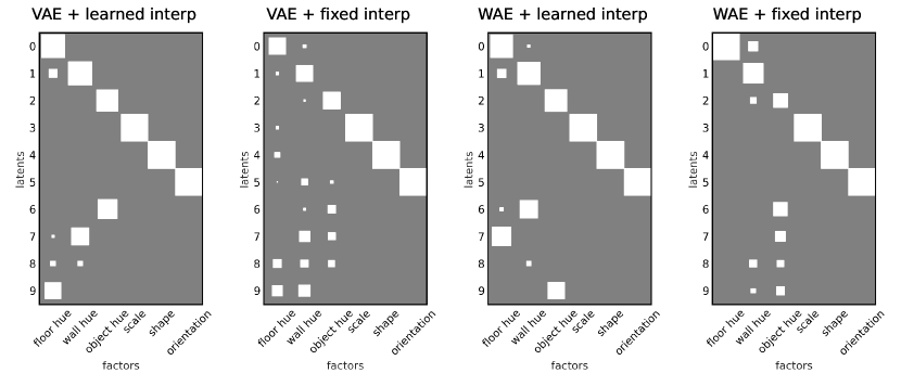
Figure 18: Visualising disentanglement for 3DShapes dataset, success condition Following Eastwood & Williams (2018), we used Hinton matrices to visualise the extent of disentanglement. Each panel shows the matrix $C$ (see Section A.5) of regression coefficients between latent variables and generative factors.

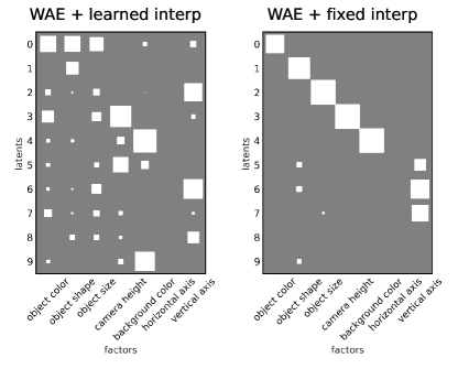
Figure 19: Visualising disentanglement for MPI3D dataset, failure condition Following Eastwood & Williams (2018), we used Hinton matrices to visualise the extent of disentanglement. Each panel shows the matrix $C$ (see Section A.5) of regression coefficients between latent variables and generative factors.

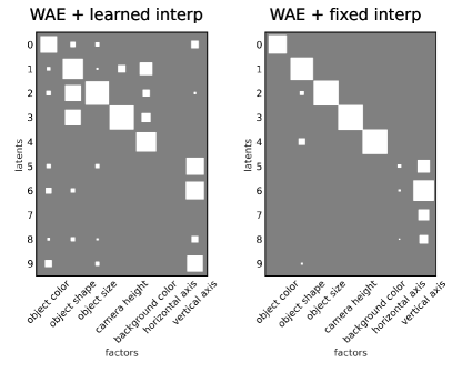
Figure 20: Visualising disentanglement for MPI3D dataset, success condition Following Eastwood & Williams (2018), we used Hinton matrices to visualise the extent of disentanglement. Each panel shows the matrix $C$ (see Section A.5) of regression coefficients between latent variables and generative factors.

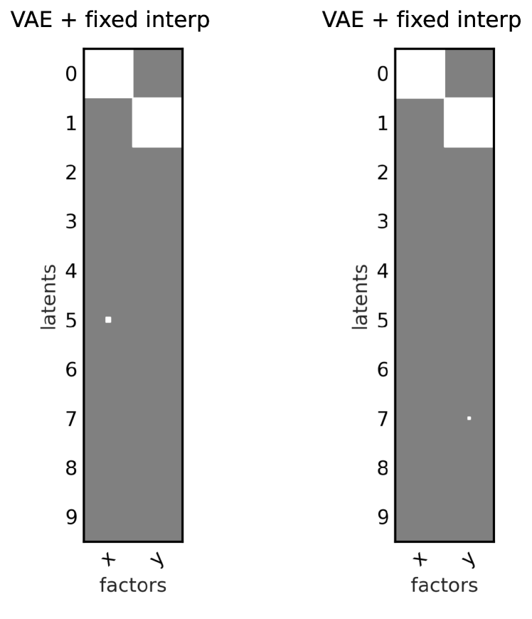
(a) Circles dataset Following Eastwood & Williams (2018), we used Hinton matrices to visualise the extent of disentanglement. Each panel shows the matrix $C$ (see Section A.5) of regression coefficients between latent variables and generative factors. Left the corner condition. The middle patch condition.

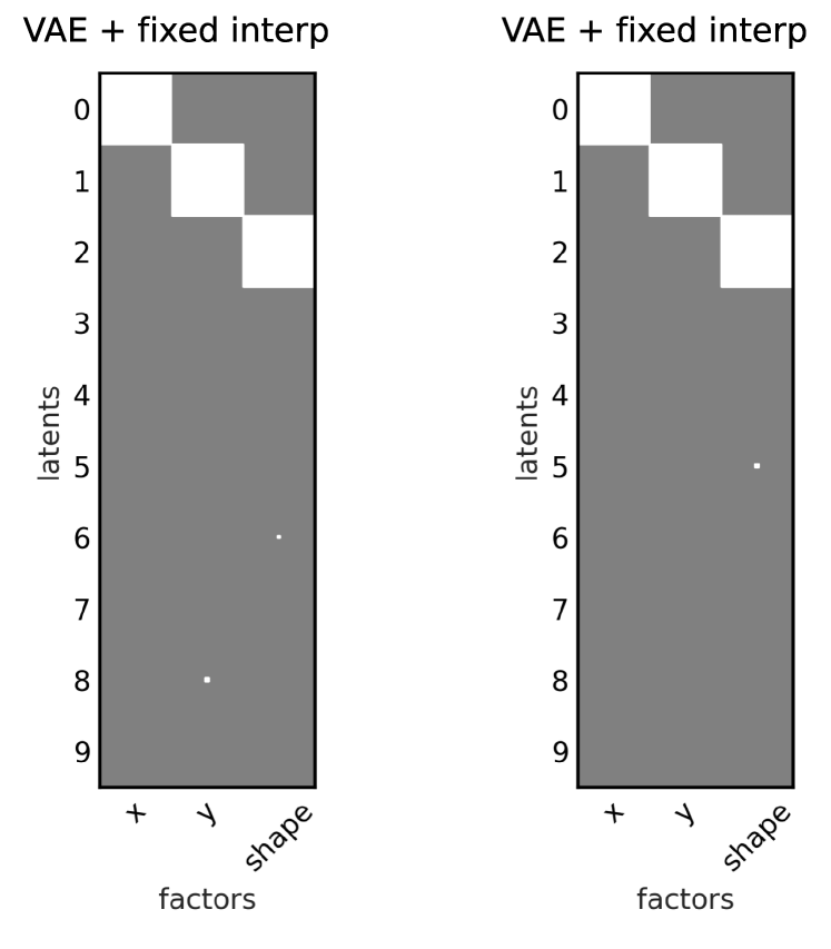
(b) Simple dataset Following Eastwood & Williams (2018), we used Hinton matrices to visualise the extent of disentanglement. Each panel shows the matrix $C$ (see Section A.5) of regression coefficients between latent variables and generative factors. Left the corner condition. The middle patch condition.

Figure 21: Visualising disentanglement for the Circles and Simple datasets

B.4 Latent visualizations

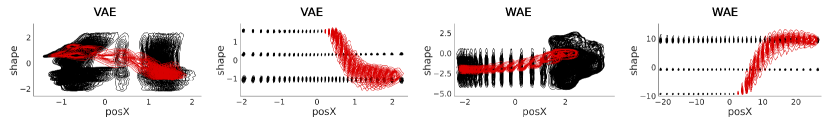
Figure 22: Visualisation of latent space for dSprites dataset. Distribution of encoded values for different combinations of shape and posX for the dSprites dataset. For models that do not disentangle well (first and third from left to right), we observe a very unstructured distribution of both training (black) and (test). Models with high disentanglement (second and fourth) show a very structured representation where it is easy to discriminate between different shapes and positions in the training set, but which diverge in the test set.

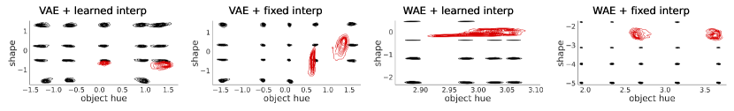
Figure 23: Visualisation of latent space for 3DShapes dataset, failure condition. Distribution of encoded values for different combinations of shape and object hue for the 3DShapes dataset. In this case, all models showed high levels of disentanglement. The factor combinations for the training set are easily distinguishable. However, models show poor generalisation in the test set. The 4th model on the right is the one that shows the best results, yet the test distributions show a signfican increase in variance and drift towards observed training data.

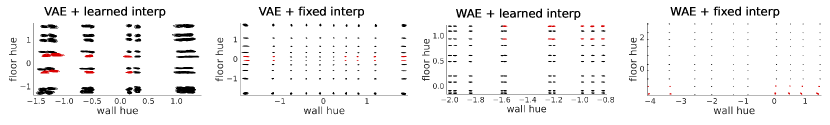
Figure 24: Visualisation of latent space for 3DShapes dataset, success condition. Distribution of encoded values for different combinations of wall hue and floor hue for the 3DShapes dataset. In this case, all models showed high levels of disentanglement. The factor combinations for the training set are easily distinguishable. As opposed to the previous condition, models show excellent generalisation to the test data.

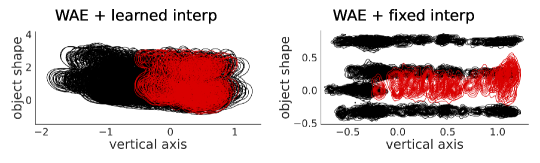
Figure 25: Visualisation of latent space for MPI3D dataset, failure condition. Distribution of encoded values for different combinations of shape and vertical axis for the MPI3D dataset. The model on the left shows poor disentanglement with the joint distribution of the best match latents for both training (black) and testing examples (red) showing significant overlap. The model on the right on the other hand achieved high disentanglement. The encoded value for each shape is easily distinguishable. The encoded angle of the arm is not as clearly separated. The test data shows a significant drift, though not as dramatic as in dSprites.

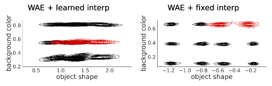
Figure 26: Visualisation of latent space for MPI3D dataset, success condition. Distribution of encoded values for different combinations of shape and vertical axis for the MPI3D dataset. The first three models from the left show poor disentanglement with the joint distribution for both training (black) and testing examples (red). The model on the right on the other hand achieved high disentanglement. The encoded value for each shape background color combination is easily distinguishable. There is no hint of drift or even increase in variance.

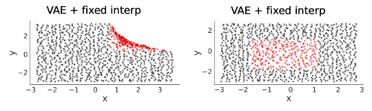
Figure 27: Visualisation of latent space for Circles dataset. We replicate the results from Watters et al.. On the left, the Spatial Broadcast Decoder shows poor generalisation when tested on the corner case. Test examples (red) bend over the closest seen training examples (black). On the right, when the excluded patch is locate in the center, the model shows excellent generalisation.

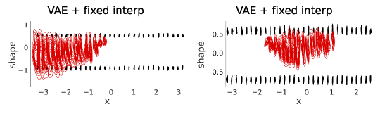
Figure 28: Visualisation of latent space for Simple dataset. We show that the Spatial Broadcast Decoder (Watters et al., 2019) fails when we introduce another shape in the middle patch position. On the left, the result for the corner case, showing again poor generalisation. The drift is similar to the one observed in dSprites: as we move away from observed positions the latent representation experience a dramatic increase in variance and shift towards the mean of the other shape. On the right, when the excluded patch is locate in the center, the model also fails as the introduction of a new shape makes turns the task too hard for the model.

References

- Battaglia et al. (2018) Battaglia, P. W., Hamrick, J. B., Bapst, V., Sanchez-Gonzalez, A., Zambaldi, V., Malinowski, M., Tacchetti, A., Raposo, D., Santoro, A., Faulkner, R., et al. Relational inductive biases, deep learning, and graph networks. arXiv preprint arXiv:1806.01261, 2018.
- Burgess & Kim (2018) Burgess, C. and Kim, H. 3d shapes dataset. https://github.com/deepmind/3dshapes-dataset/, 2018.
- Burgess et al. (2018) Burgess, C. P., Higgins, I., Pal, A., Matthey, L., Watters, N., Desjardins, G., and Lerchner, A. Understanding disentangling in $\beta$-VAE. arXiv:1804.03599 [cs, stat], April 2018. URL http://arxiv.org/abs/1804.03599. arXiv: 1804.03599.
- Chomsky (2014) Chomsky, N. Aspects of the Theory of Syntax, volume 11. MIT press, 2014.
- Duan et al. (2020) Duan, S., Matthey, L., Saraiva, A., Watters, N., Burgess, C. P., Lerchner, A., and Higgins, I. Unsupervised Model Selection for Variational Disentangled Representation Learning. arXiv:1905.12614 [cs, stat], February 2020. URL http://arxiv.org/abs/1905.12614. arXiv: 1905.12614.
- Eastwood & Williams (2018) Eastwood, C. and Williams, C. K. A framework for the quantitative evaluation of disentangled representations. In International Conference on Learning Representations, pp. 15, 2018.
- Fomin et al. (2020) Fomin, V., Anmol, J., Desroziers, S., J., K., and Tejani, A. High-level library to help with training neural networks in pytorch. https://github.com/pytorch/ignite, 2020.
- Gondal et al. (2019) Gondal, M. W., Wuthrich, M., Miladinovic, D., Locatello, F., Breidt, M., Volchkov, V., Akpo, J., Bachem, O., Schölkopf, B., and Bauer, S. On the transfer of inductive bias from simulation to the real world: a new disentanglement dataset. In Wallach, H., Larochelle, H., Beygelzimer, A., d'Alché-Buc, F., Fox, E., and Garnett, R. (eds.), Advances in Neural Information Processing Systems, volume 32. Curran Associates, Inc., 2019. URL https://proceedings.neurips.cc/paper/2019/file/d97d404b6119214e4a7018391195240a-Paper.pdf.
- Harris et al. (2020) Harris, C. R., Millman, K. J., van der Walt, S. J., Gommers, R., Virtanen, P., Cournapeau, D., Wieser, E., Taylor, J., Berg, S., Smith, N. J., Kern, R., Picus, M., Hoyer, S., van Kerkwijk, M. H., Brett, M., Haldane, A., del Río, J. F., Wiebe, M., Peterson, P., Gérard-Marchant, P., Sheppard, K., Reddy, T., Weckesser, W., Abbasi, H., Gohlke, C., and Oliphant, T. E. Array programming with NumPy. Nature, 585(7825):357–362, September 2020. doi: 10.1038/s41586-020-2649-2. URL https://doi.org/10.1038/s41586-020-2649-2.
- Higgins et al. (2017) Higgins, I., Matthey, L., Pal, A., Burgess, C., Glorot, X., Botvinick, M., Mohamed, S., and Lerchner, A. -VAE: Learning basic visual concepts with a constrained variational framework. pp. 13, 2017.
- Higgins et al. (2018a) Higgins, I., Amos, D., Pfau, D., Racaniere, S., Matthey, L., Rezende, D., and Lerchner, A. Towards a Definition of Disentangled Representations. arXiv:1812.02230 [cs, stat], December 2018a. URL http://arxiv.org/abs/1812.02230. arXiv: 1812.02230.
- Higgins et al. (2018b) Higgins, I., Pal, A., Rusu, A. A., Matthey, L., Burgess, C. P., Pritzel, A., Botvinick, M., Blundell, C., and Lerchner, A. DARLA: Improving Zero-Shot Transfer in Reinforcement Learning. arXiv:1707.08475 [cs, stat], June 2018b. URL http://arxiv.org/abs/1707.08475. arXiv: 1707.08475.
- Higgins et al. (2018c) Higgins, I., Sonnerat, N., Matthey, L., Pal, A., Burgess, C. P., Bosnjak, M., Shanahan, M., Botvinick, M., Hassabis, D., and Lerchner, A. SCAN: Learning Hierarchical Compositional Visual Concepts. arXiv:1707.03389 [cs, stat], June 2018c. URL http://arxiv.org/abs/1707.03389. arXiv: 1707.03389.
- Hummel (2000) Hummel, J. Localism as a first step toward symbolic representation. Behavioral and Brain Sciences, 23(4):480–481, December 2000. ISSN 0140-525X. doi: 10.1017/S0140525X0036335X.
- Hunter (2007) Hunter, J. D. Matplotlib: A 2d graphics environment. Computing in Science & Engineering, 9(3):90–95, 2007. doi: 10.1109/MCSE.2007.55.
- Hyvarinen & Morioka (2016) Hyvarinen, A. and Morioka, H. Unsupervised feature extraction by time-contrastive learning and nonlinear ica. Advances in Neural Information Processing Systems, 29:3765–3773, 2016.
- Kim & Mnih (2019) Kim, H. and Mnih, A. Disentangling by Factorising. arXiv:1802.05983 [cs, stat], July 2019. URL http://arxiv.org/abs/1802.05983. arXiv: 1802.05983.
- Kingma & Ba (2017) Kingma, D. P. and Ba, J. Adam: A Method for Stochastic Optimization. arXiv:1412.6980 [cs], January 2017. URL http://arxiv.org/abs/1412.6980. arXiv: 1412.6980.
- Kingma & Welling (2013) Kingma, D. P. and Welling, M. Auto-Encoding Variational Bayes. arXiv:1312.6114 [cs, stat], December 2013. URL http://arxiv.org/abs/1312.6114. arXiv: 1312.6114.
- Klaus Greff et al. (2017) Klaus Greff, Aaron Klein, Martin Chovanec, Frank Hutter, and Jürgen Schmidhuber. The Sacred Infrastructure for Computational Research. In Katy Huff, David Lippa, Dillon Niederhut, and Pacer, M. (eds.), Proceedings of the 16th Python in Science Conference, pp. 49 – 56, 2017. doi: 10.25080/shinma-7f4c6e7-008.
- Klindt et al. (2020) Klindt, D., Schott, L., Sharma, Y., Ustyuzhaninov, I., Brendel, W., Bethge, M., and Paiton, D. Towards nonlinear disentanglement in natural data with temporal sparse coding. arXiv preprint arXiv:2007.10930, 2020.
- Lin et al. (2020) Lin, Z., Thekumparampil, K., Fanti, G., and Oh, S. Infogan-cr and modelcentrality: Self-supervised model training and selection for disentangling gans. In International Conference on Machine Learning, pp. 6127–6139. PMLR, 2020.
- Locatello et al. (2020) Locatello, F., Poole, B., Rätsch, G., Schölkopf, B., Bachem, O., and Tschannen, M. Weakly-supervised disentanglement without compromises. In International Conference on Machine Learning, pp. 6348–6359. PMLR, 2020.
- Matthey et al. (2017) Matthey, L., Higgins, I., Hassabis, D., and Lerchner, A. dSprites: Disentanglement testing Sprites dataset. 2017. URL https://github.com/deepmind/dsprites-dataset/.
- McCoy et al. (2021) McCoy, R. T., Culbertson, J., Smolensky, P., and Legendre, G. Infinite use of finite means? evaluating the generalization of center embedding learned from an artificial grammar. 2021.
- Montero et al. (2020) Montero, M. L., Ludwig, C. J., Costa, R. P., Malhotra, G., and Bowers, J. The role of disentanglement in generalisation. In International Conference on Learning Representations, 2020.
- Munkres (1957) Munkres, J. Algorithms for the assignment and transportation problems. Journal of the society for industrial and applied mathematics, 5(1):32–38, 1957.
- Paszke et al. (2019) Paszke, A., Gross, S., Massa, F., Lerer, A., Bradbury, J., Chanan, G., Killeen, T., Lin, Z., Gimelshein, N., Antiga, L., Desmaison, A., Kopf, A., Yang, E., DeVito, Z., Raison, M., Tejani, A., Chilamkurthy, S., Steiner, B., Fang, L., Bai, J., and Chintala, S. Pytorch: An imperative style, high-performance deep learning library. In Wallach, H., Larochelle, H., Beygelzimer, A., d'Alché-Buc, F., Fox, E., and Garnett, R. (eds.), Advances in Neural Information Processing Systems 32, pp. 8024–8035. Curran Associates, Inc., 2019.
- Schölkopf et al. (2021) Schölkopf, B., Locatello, F., Bauer, S., Ke, N. R., Kalchbrenner, N., Goyal, A., and Bengio, Y. Toward causal representation learning. Proceedings of the IEEE, 109(5):612–634, 2021.
- Schott et al. (2021) Schott, L., von Kügelgen, J., Träuble, F., Gehler, P., Russell, C., Bethge, M., Schölkopf, B., Locatello, F., and Brendel, W. Visual representation learning does not generalize strongly within the same domain. arXiv preprint arXiv:2107.08221, 2021.
- Smolensky (1988) Smolensky, P. Connectionism, constituency, and the language of thought. University of Colorado at Boulder, 1988.
- Tolstikhin et al. (2017) Tolstikhin, I., Bousquet, O., Gelly, S., and Schoelkopf, B. Wasserstein auto-encoders. arXiv preprint arXiv:1711.01558, 2017.
- van Steenkiste et al. (2019) van Steenkiste, S., Schmidhuber, J., Locatello, F., and Bachem, O. Are Disentangled Representations Helpful for Abstract Visual Reasoning? pp. 14, 2019.
- Von Humboldt et al. (1999) Von Humboldt, W., von Humboldt, W. F., et al. Humboldt:’On language’: On the diversity of human language construction and its influence on the mental development of the human species. Cambridge University Press, 1999.
- Waskom (2021) Waskom, M. L. seaborn: statistical data visualization. Journal of Open Source Software, 6(60):3021, 2021. doi: 10.21105/joss.03021. URL https://doi.org/10.21105/joss.03021.
- Watters et al. (2019) Watters, N., Matthey, L., Burgess, C. P., and Lerchner, A. Spatial Broadcast Decoder: A Simple Architecture for Learning Disentangled Representations in VAEs. arXiv:1901.07017 [cs, stat], August 2019. URL http://arxiv.org/abs/1901.07017. arXiv: 1901.07017.