The Probabilistic Normal Epipolar Constraint for Frame-To-Frame Rotation Optimization under Uncertain Feature Positions

Abstract

The estimation of the relative pose of two camera views is a fundamental problem in computer vision. Kneip et al. proposed to solve this problem by introducing the normal epipolar constraint (NEC). However, their approach does not take into account uncertainties, so that the accuracy of the estimated relative pose is highly dependent on accurate feature positions in the target frame. In this work, we introduce the probabilistic normal epipolar constraint (PNEC) that overcomes this limitation by accounting for anisotropic and inhomogeneous uncertainties in the feature positions. To this end, we propose a novel objective function, along with an efficient optimization scheme that effectively minimizes our objective while maintaining real-time performance. In experiments on synthetic data, we demonstrate that the novel PNEC yields more accurate rotation estimates than the original NEC and several popular relative rotation estimation algorithms. Furthermore, we integrate the proposed method into a state-of-the-art monocular rotation-only odometry system and achieve consistently improved results for the real-world KITTI dataset.

Figure 1: Illustration of the proposed method. The feature correspondences (left: lines) exhibit different position error distributions (left: ellipses). In contrast to the NEC [35], our probabilistic normal epipolar constraint (PNEC) correctly accounts for the uncertainty and the geometry of the problem (middle) through a weighted (NEC) vs. unweighted (PNEC) averaging scheme (right). The NEC weighs all residuals equally (right: dash-dotted blue line), so that valuable information is lost. In contrast, our PNEC takes into account a proper weighting of individual residuals (right: dashed green line). Relative pose estimation with the PNEC instead of the NEC reduces the rotational-only versions of the $\text{RPE}_{1}$ and the $\text{RPE}_{n}$ error by up to $42\%$ and $55\%$ on the KITTI dataset [21], respectively.

1 Introduction

Extracting the 3D geometry of a scene from images is a long-standing problem in computer vision and has numerous applications, including augmented and virtual reality, autonomous driving, or robots that can help with everyday life. One key component of many such approaches is the estimation of the relative pose between two viewpoints of a scene. For example, relative pose estimation is the foundation of geometric vision algorithms like structure from motion (SfM) or visual odometry (VO). Global SfM pipelines rely on accurate pairwise relative poses for use as fixed measurements in global motion averaging [24, 49]. In VO, relative pose estimation is used to construct a trajectory from a stream of images. Like for all odometry systems, small errors in the relative pose estimation lead to a drift in VO.

The most widely used concept for relative pose estimation is the essential matrix [44] in the calibrated case, or the fundamental matrix [26] in the general case. Respective approaches rely on correspondences between feature points, and are generally known to provide fast and accurate results [25]. However, approaches based on the essential matrix suffer from fundamental problems, with the most prominent being solution multiplicity [18, 26] and planar degeneracy [34]. To address such issues, often it is necessary to consider more involved solution strategies, which also lead to even more accurate relative poses as shown by Kneip et al. [34] and in this work.

To this end, Kneip et al. [35] proposed a constraint that avoids these problems. Their epipolar plane normal coplanarity constraint (in later works just normal epipolar constraint, NEC) allows the estimation of the rotation independent of the translation. A later work by Kneip and Lynen [34] provides a fast and reliable eigenvalue-based solver for the NEC, which allows for real-time relative pose estimation. This approach has been incorporated into rotation-only VO systems that estimate the rotation independent of the translation and has led to promising results [10, 40].

Yet, like many VO systems, neither of them considers the quality of the correspondences. After removing outliers from the feature matches, every match contributes equally to the final result. However, two-dimensional feature correspondences exhibit different error distributions depending on the content of the image and the specific method used to extract the correspondences, which can be seen in Fig. 2. A correspondence lying on an edge is accurately localized perpendicular to the edge and possesses higher position uncertainty parallel to it. This fine-grained information about the quality of the matches is completely ignored. It has been shown that considering the uncertainty is beneficial for fundamental matrix estimation [6]. While Kanazawa et al. [31] argue that the uncertainty needs to be sufficiently inhomogeneous to see the aforementioned benefit, our experiments show that the PNEC improves over the NEC even for homogeneous uncertainty due to the geometry of the problem.

The main objective of our work is to improve the accuracy of rotation estimation techniques. We achieve this based on the following technical contributions:

• We introduce the novel probabilistic normal epipolar constraint (PNEC), see Fig. 1, which for the first time makes it possible to incorporate uncertainty information into the normal epipolar constraint (NEC).

• We propose an efficient two-stage optimization strategy for the PNEC that achieves real-time performance.

• We analyse singularities in the PNEC energy function and address them with a simple regularization scheme.

• Experimentally, we compare our PNEC to several popular relative pose estimation algorithms, namely 8pt [25], 7pt [26], Stewenius 5pt [58], Nistér 5pt [52], and NEC [34], and demonstrate that our PNEC delivers more accurate rotation estimates. Moreover, we integrate our PNEC into a visual odometry system and achieve state-of-the-art results on real-world data.

• We publish the code for all experiments to facilitate future research.

2 Related Work

The focus of this paper is the integration of feature position uncertainties into frame-to-frame rotation estimation and the application to visual odometry. Hence, we restrict our discussion of related work to relative pose estimation, uncertainty for feature correspondences, and visual odometry. For a broader overview we refer the reader to the excellent books by Szeliski [59] and by Hartley and Zisserman [26] and to more topic-specific overview papers [61, 7].

Relative Pose Estimation. Estimating the relative pose between two viewpoints is a long-standing problem in computer vision with the first known solution proposed in 1913 by Kruppa [36]. Most methods either rely on previously computed feature correspondences (feature-based) or directly consider the intensity differences between the two images (direct). While direct methods have recently shown promising results [16, 15], they are currently limited to images that exhibit photo consistency and hence cannot be used for general problems, e.g. structure from motion. Feature-based methods are considerably more robust to viewpoint and appearance changes. Therefore, we use feature correspondences within this paper.

Given feature correspondences, many methods [44, 52, 57, 42, 37] estimate the essential matrix in the case of a calibrated camera, or the fundamental matrix in the general case. Nistér [52] proposes a minimal solution using polynomials and root bracketing, while the solver proposed by Longuet-Higgins [44] is linear and requires careful normalization for good performance [25]. Alternatively, the relative pose can be estimated directly using quaternions [17].

The essential matrix constraint deteriorates in zero-translation situations without noise, due to it being a zero matrix. Most essential-matrix-based algorithms estimate the correct motion only implicitly [34]. To address this problem, recent works have proposed algorithms that can estimate the rotation independent of the translation [43, 35]. Our work is based on the normal epipolar constraint (NEC) proposed by Kneip et al. [35] and the direct optimization scheme proposed in a follow-up paper [34]. Briales et al. [5] show how to obtain the global minimum for the NEC, however, their Shor relaxation is not applicable to our non-polynomial energy function.

Uncertainty for Feature Correspondences. Kanade-Lucas-Tomasi (KLT) tracks [46, 60] are widely used, and the position uncertainty has been extensively investigated [20, 56, 55, 67]. Based on the unscented transform [62], the position uncertainty has also been integrated directly into the KLT tracking [14]. Zeisl et al. [66] have shown a method to obtain anisotropic and inhomogeneous covariances for SIFT [45] and SURF [2] features.

The integration of the position uncertainty into the alignment problem has been studied from a statistical perspective [29, 30], in the photogrammetry community [48], as well as in the computer vision community [6, 31]. Brooks et al. [6] show that covariance information can be used beneficially if the estimated covariance is sufficiently accurate. Kanazawa et al. [31] question the practical use of covariance information if the covariance matrices are too similar and nearly isotropic, however, Fig. 2 shows clearly that the covariance matrices for real-world data are highly inhomogeneous and anisotropic.

Visual Odometry Systems. Most VO approaches utilize 3D-to-2D correspondences together with a sliding window formulation. Still, relative pose estimation is commonly used during initialization [50] and has been shown to provide excellent results on its own [12, 13]. Based on different solutions to the correspondence problem many visual odometry systems have been proposed. They include PTAM [32] and ORB-SLAM [50, 51] with indirect features, approaches with KLT-tracks [63], as well as direct methods like LSD-SLAM [16] and DSO [15]. Common among these approaches is a deteriorating performance for pure rotation without inertial data.

Multiple rotation-only approaches that are robust against pure rotation have been proposed recently [11, 10, 40]. Choncha et al. [11] use the NEC to initialize a scale-consistent map even for purely rotational motion. Chng et al. [10] and Lee and Civera [40] use rotation averaging and rotation-only bundle adjustment on the basis of the NEC to further improve their results, respectively. While these approaches show promising results on existing datasets, neither of them utilizes uncertainty information of feature correspondences in their system. We base our VO evaluation on MRO [10].

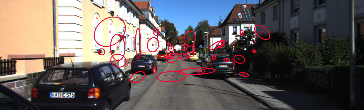
Figure 2: Covariance ellipses for position uncertainties in KITTI seq. 07. The tracks are generated with KLT tracking. Our PNEC correctly considers such anisotropic inhomogeneous error distributions. For visualization purposes only a sub-image with sub-sampled and enlarged covariance ellipses is shown.

3 Probabilistic Normal Epipolar Constraint

The normal epipolar constraint (NEC) [35] enforces the coplanarity of epipolar plane normal vectors constructed from feature correspondences. However, feature correspondences exhibit different error distributions that are not accounted for in the NEC. For example, an edge-like feature is well-localized perpendicular to the edge but not parallel to it, which is also known as the aperture problem. Fig. 2 clearly shows the anisotropicity and inhomogeneity of the position distributions. Moreover, it is well-known that correspondences in all areas of the image are required to sufficiently constrain the 3D geometry [15, 50] and thus we cannot simply discard feature points. To address this problem, we propose the probabilistic normal epipolar constraint (PNEC), which is able to take into account the uncertainty of feature positions by associating an anisotropic covariance matrix to each feature point.

Notation. Vectors are denoted by bold lowercase letters (e.g. $\boldsymbol{f}$) and matrices by bold uppercase letters (e.g. $\boldsymbol{\Sigma}$). The hat operator applied to a vector $\boldsymbol{u}\in\mathbb{R}^{3}$ gives a skew-symmetric matrix $\hat{\boldsymbol{u}}\in\mathbb{R}^{3\times 3}$ that computes the cross product between two vectors, i.e. $\boldsymbol{u}\times\boldsymbol{v}=\hat{\boldsymbol{u}}\boldsymbol{v}$. The superscript ^⊤ denotes the transpose. A rigid-body transformation is represented by a rotation matrix $\boldsymbol{R}\in SO(3)$ and a unit length translation $\boldsymbol{t}\in\mathbb{R}^{3}$ ($\|\boldsymbol{t}\|=1$ is imposed since the two-view problem is scale-invariant).

3.1 Background – NEC

Figure 3: Geometry of the normal epipolar constraint (NEC) [35]. Feature correspondences are given by pairs of unit bearing vectors $\boldsymbol{f}_{i}$ and $\boldsymbol{f}^{\prime}_{i}$ in the host frame ($O$) and target frame ($O^{\prime}$), respectively. Each pair of bearing vectors spans an epipolar plane (yellow, orange, red), and has an associated normal vector $\boldsymbol{n}_{i}$ given in Eq. 1. All epipolar planes intersect in the line defined by the translation $\boldsymbol{t}$ (dashed line). The normal vectors span the epipolar normal plane (gray) that is orthogonal to $\boldsymbol{t}$. For visual clarity we show only three feature correspondences.

In the following we summarize the main idea of the NEC proposed in [35]. Given are a host frame and a target frame that observe at least five feature correspondences that are defined by pairs of unit bearing vectors $\boldsymbol{f}_{i}$ and $\boldsymbol{f}^{\prime}_{i}$ in the host and target frame, respectively (see Fig. 3). A 3D point $\boldsymbol{x}^{\prime}$ in the target frame is transformed into the host frame by applying the relative rotation $\boldsymbol{R}$ and translation $\boldsymbol{t}$ s.t. ${\boldsymbol{x}=\boldsymbol{R}\boldsymbol{x}^{\prime}+\boldsymbol{t}}$. In the ideal, error-free case, a single feature correspondence, together with the two viewpoints, creates an epipolar plane, represented by its normal vector

$$\boldsymbol{n}_{i}=\boldsymbol{f}_{i}\times\boldsymbol{R}\boldsymbol{f}^{\prime}_{i}.$$ (1)

All normal vectors are orthogonal to the translation and they span the epipolar normal plane.

The rotation is estimated by enforcing the coplanarity of the normal vectors. The residual of the model is given by the normalized epipolar error

$$e_{i}=|\boldsymbol{t}^{\top}\boldsymbol{n}_{i}|\,,$$ (2)

i.e. the Euclidean distance of a normal vector to the epipolar normal plane. An energy function

$$E(\boldsymbol{R},\boldsymbol{t})=\sum_{i}e_{i}^{2}=\sum_{i}|\boldsymbol{t}^{\top}(\boldsymbol{f}_{i}\times\boldsymbol{R}\boldsymbol{f}^{\prime}_{i})|^{2}$$ (3)

is constructed from the residuals. For a more detailed derivation, we kindly refer the reader to the original paper [35] or the recent paper by Lee and Civera [39], which offers numerous geometric interpretations of the NEC.

3.2 Deriving the PNEC

The probabilistic normal epipolar constraint (PNEC) extends the NEC by incorporating uncertainty. To be more specific, the PNEC allows the use of the anisotropic and inhomogeneous nature of the uncertainty of the feature position in the energy function. The feature position error is considered in the target frame as shown in Fig. 1 and we assume that the position error follows a 2D Gaussian distribution in the image plane with a known covariance matrix $\boldsymbol{\Sigma}_{2\text{D},i}$ per feature. In App. C we show how the covariance matrix can be extracted for KLT tracks from the KLT energy function using Laplace’s approximation [4].

Given the 2D covariance matrix of the feature position in the target frame $\boldsymbol{\Sigma}_{2\text{D},i}$, we propagate it through the unprojection function using the unscented transform [62] in order to obtain the 3D covariance matrix $\boldsymbol{\Sigma}_{i}$ of the bearing vector $\boldsymbol{f}^{\prime}_{i}$. Using the unscented transform ensures full-rank covariance matrices after the transform. We derive the details of the unscented transform in App. D and show qualitative examples.

Propagating this distribution to the normalized epipolar error gives the probabilistic distribution of the residual. Due to the linearity of the transformations, the distribution of the residual is a univariate Gaussian distribution $\mathcal{N}(0,\sigma_{i}^{2})$, with variance

$$\sigma_{i}^{2}(\boldsymbol{R},\boldsymbol{t})=\boldsymbol{t}^{\top}\hat{\boldsymbol{f}_{i}}\boldsymbol{R}\boldsymbol{\Sigma}_{i}\boldsymbol{R}^{\top}\hat{\boldsymbol{f}_{i}}{}^{\top}\boldsymbol{t}\,.$$ (4)

We integrate this variance into the cost-function of the NEC so that the Euclidean distance becomes the Mahalonobis distance [9] and define the PNEC Energy Function

$$E_{P}(\boldsymbol{R},\boldsymbol{t})=\sum_{i}\frac{e_{i}^{2}}{\sigma_{i}^{2}}=\sum_{i}\frac{|\boldsymbol{t}^{\top}(\boldsymbol{f}_{i}\times\boldsymbol{R}\boldsymbol{f}^{\prime}_{i})|^{2}}{\boldsymbol{t}^{\top}\hat{\boldsymbol{f}_{i}}\boldsymbol{R}\boldsymbol{\Sigma}_{i}\boldsymbol{R}^{\top}\hat{\boldsymbol{f}_{i}}{}^{\top}\boldsymbol{t}}\,,$$ (5)

which results in a weighted optimization problem. In App. E we show a geometric interpretation of the above derivation.

4 Optimization

To optimize the PNEC energy function Eq. 5, we propose a two-stage optimization scheme consisting of an alternating iterative optimization and a joint refinement. We propose this two-stage approach since the eigenvalue-based optimization of the NEC [34] cannot be naively applied to our derived PNEC energy function, which we show in Sec. 4.1. The whole PNEC optimization is given in Alg. 1 and we detail the first stage in Sec. 4.2 & Sec. 4.3, and the second stage in Sec. 4.4.

4.1 Background – Optimizing the NEC

Following [34], the NEC energy function Eq. 3 is re-written as ${E(\boldsymbol{R},\boldsymbol{t})=\boldsymbol{t}^{\top}\boldsymbol{M}(\boldsymbol{R})\boldsymbol{t}}$ using the (symmetric and positive-semidefinite) Gramian matrix

$$\boldsymbol{M}(\boldsymbol{R})=\sum_{i}(\boldsymbol{f}_{i}\times\boldsymbol{R}\boldsymbol{f}^{\prime}_{i})(\boldsymbol{f}_{i}\times\boldsymbol{R}\boldsymbol{f}^{\prime}_{i})^{\top}\,.$$ (6)

Because the energy is a quadratic form in the unit vector $\boldsymbol{t}$, the optimization over the translation $\boldsymbol{t}$ can be carried out analytically, i.e.

$$\min_{\begin{subarray}{c}\boldsymbol{R}\in\text{SO}(3)\\ \boldsymbol{t}:\;\|\boldsymbol{t}\|=1\end{subarray}}\boldsymbol{t}^{\top}\boldsymbol{M}(\boldsymbol{R})\boldsymbol{t}\;=\min_{\boldsymbol{R}\in\text{SO}(3)}\operatorname{\lambda}_{\text{min}}(\boldsymbol{M}(\boldsymbol{R}))\,.$$ (7)

The eigenvector corresponding to the smallest eigenvalue $\lambda_{\text{min}}$ of $\boldsymbol{M}(\boldsymbol{R})$ minimizes the Rayleigh quotient $\boldsymbol{t}^{\top}\boldsymbol{M}(\boldsymbol{R})\boldsymbol{t}$ over all unit-length vectors $\boldsymbol{t}$. The constructed sub-problem is then optimized over the rotation $\boldsymbol{R}$ using the Levenberg-Marquardt algorithm [41, 47], whereas the translation $\boldsymbol{t}$ is obtained by solving an eigenvalue problem.

1 Initialize weights $\tilde{\sigma}_{i,0}\leftarrow 1\;\forall i$

for $s\leftarrow 1$ to $S$ do

      2 Optimize over $\boldsymbol{R}$ (cf. Sec. 4.3)

       $\boldsymbol{R}_{s}\leftarrow\operatorname{Opt}_{\boldsymbol{R}}\;\operatorname{\lambda}_{\text{min}}(\boldsymbol{M}_{P}(\boldsymbol{R};\{\tilde{\sigma}_{i,s-1}\}_{i}))$

      [1.1ex]

      3Optimize over $\boldsymbol{t}$ (cf. Sec. 4.2)

       $\boldsymbol{t}_{s}\leftarrow\operatorname{Opt}_{\boldsymbol{t}}\;E_{P}(\boldsymbol{R}_{s},\boldsymbol{t})$

      [1.1ex]

      4Update the weights (cf. Eq. 4)

       $\tilde{\sigma}_{i,s}\leftarrow\sigma_{i}(\boldsymbol{R}_{s},\boldsymbol{t}_{s})\;\forall i$

end for

5Joint Refinement (cf. Sec. 4.4) using $(\boldsymbol{R}_{S},\boldsymbol{t}_{S})$ as starting value

$\boldsymbol{R}^{\ast},\boldsymbol{t}^{\ast}\leftarrow\operatorname{Opt}_{\boldsymbol{R},\boldsymbol{t}}E_{P}(\boldsymbol{R},\boldsymbol{t})$

Algorithm 1 PNEC Optimization Scheme

4.2 Optimizing the PNEC - Translation

The PNEC energy function Eq. 5 is the sum of generalized Rayleigh quotients in the translation $\boldsymbol{t}$, and thus the optimum is not simply given by an eigenvalue as for the NEC. Optimizing the sum of GRQs over the unit sphere has recently been studied in the context of data science and wireless communications [68, 69, 3], and it has been shown by Zhang et al. [69] that the self-consistent-field (SCF) algorithm [27] outperforms generic manifold optimization methods.

Since the sum of GRQs can exhibit many local minima [3], and thus the SCF iteration is not guaranteed to converge to a global optimum, we propose a simple, yet effective globalization strategy. To this end, we make use of the intrinsic low dimension of the unit sphere in $\mathbb{R}^{3}$ by sampling evenly distributed initial points $\boldsymbol{t}_{k}$ efficiently using the Fibonacci lattice [22]. We then pick the point with the lowest objective function and apply the SCF iteration for $N$ steps. Due to the inherent parallelism, the resulting optimization procedure can be implemented efficiently. We present the effectiveness of the globalization strategy, as well as technical details for the SCF iteration, in the supplementary material in App. G and Tab. 5.

4.3 Optimizing the PNEC - Rotation

Kneip and Lynen [34] have shown how to optimize Eq. 7 efficiently using the Levenberg-Marquardt algorithm with the rotation parametrized based on the Cayley transformation [8]. To account for the weights in the PNEC energy function Eq. 5, we employ an optimization scheme similar to the popular iteratively reweighted least squares (IRLS) algorithm [38]. Specifically, given a previous estimate of the rotation and translation $(\boldsymbol{R}_{p},\boldsymbol{t}_{p})$, we compute fixed weights $\tilde{\sigma}_{i}=\sigma_{i}(\boldsymbol{R}_{p},\boldsymbol{t}_{p})$ for all $i$, and define the weighted matrix

$$\boldsymbol{M}_{P}(\boldsymbol{R};\{\tilde{\sigma}_{i}\}_{i})=\sum_{i}\frac{(\boldsymbol{f}_{i}\times\boldsymbol{R}\boldsymbol{f}^{\prime}_{i})(\boldsymbol{f}_{i}\times\boldsymbol{R}\boldsymbol{f}^{\prime}_{i})^{\top}}{\tilde{\sigma}_{i}^{2}}$$ (8)

that depends only on the rotation $\boldsymbol{R}$. The rotation is obtained by finding $\boldsymbol{R}$ such that the smallest eigenvalue of $\boldsymbol{M}_{P}(\boldsymbol{R};\{\tilde{\sigma}_{i}\}_{i})$ is minimal. After doing so based on the optimizer of Kneip and Lynen [34], the weights $\{\tilde{\sigma}_{i}\}_{i}$ are updated with new $\boldsymbol{R},\boldsymbol{t}$.

4.4 Optimizing the PNEC - Joint Refinement

After the first stage we improve the result using joint refinement. Specifically, we use a least-squares optimization strategy, which is effective for finding a local optimum of the energy function given a good starting point [53]. For the PNEC we optimize over

$$E_{P}(\boldsymbol{R},\boldsymbol{t})=\sum_{i}\left(\frac{\boldsymbol{t}^{\top}(\boldsymbol{f}_{i}\times\boldsymbol{R}\boldsymbol{f}^{\prime}_{i})}{\sqrt{\boldsymbol{t}^{\top}\hat{\boldsymbol{f}_{i}}\boldsymbol{R}\boldsymbol{\Sigma}_{i}\boldsymbol{R}^{\top}\hat{\boldsymbol{f}_{i}}{}^{\top}\boldsymbol{t}}}\right)^{2}\,,$$ (9)

the least-squares formulation of the constraint. The Levenberg-Marquardt algorithm optimizes the objective function in the rotation $\boldsymbol{R}$ and translation $\boldsymbol{t}$ simultaneously and uses the solution of the first stage as the starting value. Because $\boldsymbol{R}$ is a rotation matrix, we use manifold optimization [28] to optimize over the special orthogonal group $\text{SO}(3)$. For the translation $\boldsymbol{t}$ we use spherical coordinates with the radius fixed to one in order to ensure that $\|\boldsymbol{t}\|=1$ holds. We would like to highlight that this joint refinement is different from bundle adjustment. Most notably, it does not need to calculate the 3D position of the features.

4.5 Singularities of the PNEC

Figure 4: Visualization of the NEC, the PNEC, and the PNEC with the regularization proposed in Sec. 4.5. The plot shows $\boldsymbol{t}$ in a neighborhood of $\boldsymbol{f}$ (in polar coordinates), where the center of the circle corresponds to $\boldsymbol{t}=\boldsymbol{f}$. For $\boldsymbol{t}=\boldsymbol{f}$, the PNEC shows a finite discontinuity, for which the limit depends on the direction. Our regularization eliminates this singularity while also maintaining the overall shape of the energy function.

The PNEC energy function Eq. 5 has a singularity if the translation $\boldsymbol{t}$ is parallel to a bearing vector $\boldsymbol{f}_{i}$ because the variance $\sigma_{i}^{2}$ vanishes due to $\hat{\boldsymbol{f}_{i}}\boldsymbol{t}=\boldsymbol{f}_{i}\times\boldsymbol{t}=\boldsymbol{0}$. On the other hand, the numerator involves the same term and thus the energy function is bounded and possesses a finite discontinuity, as illustrated in Fig. 4. In App. F we present the derivation of the directional limit of the energy function.

While the discontinuity is finite and less problematic than an infinite discontinuity, it still poses challenges. First, in contrast to the function values, the derivatives of the energy function are not bounded, which is problematic for the joint refinement. Second, the matrix $\boldsymbol{M}_{P}$, unlike the energy function, includes $\hat{\boldsymbol{f}_{i}}\boldsymbol{t}$ only in its denominator not the numerator. Hence $\boldsymbol{M}_{P}$ tends to infinity for $\boldsymbol{t}\to\boldsymbol{f}_{i}$. To address these issues, we consider a variance of the form $\sigma_{i}^{\prime}{}^{2}=\sigma_{i}^{2}+c$ with regularization constant $c>0$. Fig. 4 shows the effect that the regularizer has on the energy function.

(a) Experiment w/ translation: $e_{\text{rot}}$

(b) Experiment w/ translation: $e_{\text{t}}$

(c) Experiment w/o translation: $e_{\text{rot}}$

Figure 5: Experiments for omnidirectional cameras. Results are averaged over 10 000 random instantiations for anisotropic inhomogeneous noise over different noise intensities. Our PNEC consistently leads to smaller errors compared to the NEC [34] for all noise levels. This holds for rotation and translation estimates in the general case in 5(a) and 5(b), respectively, as well as the rotation in the zero-translation case in 5(c).

(a) Experiment w/ translation: $e_{\text{rot}}$

(b) Experiment w/ translation: $e_{\text{t}}$

(c) Experiment w/o translation: $e_{\text{rot}}$

Figure 6: Experiments for pinhole cameras. Results are averaged over 10 000 random instantiations for anisotropic inhomogeneous noise over different noise intensities. As for an omnidirectional camera in Fig. 5, our PNEC consistently leads to smaller errors compared to the NEC [34]. For a pinhole camera the average errors are higher for both methods in comparison to an omnidirectional camera. The experiments show that our PNEC is viable for the two most common camera types.

5 Evaluation

We evaluate the performance of the PNEC and compare it to the original NEC on simulated data as well as in a visual odometry setting on real world data. On the simulated data, the proposed PNEC achieves better results than the NEC and several other popular relative pose estimation algorithms. On KITTI we compare our approach to the MRO algorithm [10] that uses the NEC for rotation estimation. For evaluating the PNEC we replace the ORB features in MRO with Kanade-Lucas-Tomasi (KLT) tracks [46, 60], which allow for uncertainty extraction as discussed in Sec. 3.2, and the NEC with the PNEC.

In App. I, a more detailed analysis including translational errors shows that compared to the NEC the PNEC is not only significantly more accurate on average, but also more consistent. An ablation study on KITTI (cf. App. M) demonstrates that all stages of our optimization scheme are essential for best results. We furthermore detail all hyperparameter choice and detail the experimental protocol for reproducibility (cf  App. H).

5.1 Frame-to-Frame Simulation

	Omnidirectional									Pinhole
	w/ t						w/o t			w/ t						w/o t
Noise level [px]	0.5		1.0		1.5		0.5	1.0	1.5	0.5		1.0		1.5		0.5	1.0	1.5
Metric [degree]	$e_{\text{rot}}$	$e_{\text{t}}$	$e_{\text{rot}}$	$e_{\text{t}}$	$e_{\text{rot}}$	$e_{\text{t}}$	$e_{\text{rot}}$	$e_{\text{rot}}$	$e_{\text{rot}}$	$e_{\text{rot}}$	$e_{\text{t}}$	$e_{\text{rot}}$	$e_{\text{t}}$	$e_{\text{rot}}$	$e_{\text{t}}$	$e_{\text{rot}}$	$e_{\text{rot}}$	$e_{\text{rot}}$
7pt [26]/8pt [25]	0.19	1.76	0.26	2.36	0.33	2.64	0.10	0.15	0.20	0.62	4.64	0.89	6.09	1.07	6.74	0.17	0.23	0.28	+95%
Stewenius 5pt [58]	0.23	2.34	0.30	2.97	0.37	3.38	0.18	0.30	0.33	0.61	3.14	0.71	4.04	0.89	4.57	0.46	0.64	0.77	+137%
Nistér 5pt [52]	1.61	6.82	1.64	7.55	1.92	8.42	0.29	0.39	0.42	3.26	8.72	3.46	9.80	3.76	10.39	0.51	0.67	0.83	+643%
NEC [34]	0.11	1.90	0.15	2.10	0.17	2.11	0.11	0.15	0.18	0.25	2.41	0.34	2.78	0.41	2.91	0.19	0.25	0.29	+24%
PNEC (Ours)	0.08	1.29	0.12	1.60	0.14	1.66	0.09	0.13	0.15	0.20	2.06	0.28	2.38	0.34	2.54	0.15	0.21	0.25

Table 1: Rotation and translation error for different algorithms. Results for omnidirectional and pinhole cameras for experiments with and without translation over different noise levels for anisotropic and inhomogenous noise. Errors are averaged over 10 000 random problems each with 10 points. For experiments without translation (W/O T) only $e_{\text{rot}}$ is reported, due to $e_{\text{t}}$ not being defined for zero translation. For all other algorithms apart from our PNEC we use the implementations from OpenGV [33]. (7pt) falls back to (8pt) for the non-minimal number of 10 correspondences. Our PNEC consistently achieves the best results, outperforming the NEC and several popular relative pose estimation algorithms. The last column gives the average error increase compared to the PNEC.

With the simulated experiments we evaluate the performance of the PNEC in a frame-to-frame setting. The experiments consist of randomly generated problems of two frames with known correspondences. We use

$$e_{\text{rot}} :=\angle(\boldsymbol{R}^{\top}\tilde{\boldsymbol{R}}),~{}\text{and}$$ (10)

$$e_{\text{t}} :=\arccos{(\boldsymbol{t}^{\top}\tilde{\boldsymbol{t}})}$$ (11)

as error metrics between the ground truth $\boldsymbol{R},\boldsymbol{t}$ and the estimated values $\tilde{\boldsymbol{R}},\tilde{\boldsymbol{t}}$, where $\angle(\cdot)$ returns the angle of the rotation matrix.

Omnidirectional Camera. In this experiment we follow the experimental outline proposed by Kneip and Lynen [34] closely. We differ from the original experiments in the following ways: we only add noise to the points in the second frame; to compensate for the lack of noise in the first frame, we scale the standard deviation by a factor of $2$; we recreate the experiment with different noise types based on the classification by Brooks et al. [6] and generate individual covariance matrices for each point. A detailed description of how the matrices are generated can be found in App. I. To show the effectiveness of the PNEC still holds even for pure rotation, we repeat the experiment with the translational difference fixed to zero.

Fig. 5 shows the results for anisotropic inhomogeneous noise for both experiments. The PNEC achieves consistently better results for the rotation over all noise levels in both experiments.

Pinhole Camera. Since most cameras are modeled as pinhole cameras we also repeat the previous experiments for pinhole cameras. The generation of the frames stays the same. Points are sampled in viewing direction of the coordinate system of the first frame. The points are projected into the world coordinate system and then into the two frames using a pinhole camera model. The noise offset is added in the image plane. As with the omnidirectional camera experiment, we repeat this experiment for pure rotation.

Fig. 6 shows the results for the pinhole camera experiment for anisotropic inhomogeneous noise. While the overall error for both methods is slightly higher for pinhole cameras than for omnidirectional cameras, the PNEC still outperforms the NEC consistently.

Tab. 1 gives a quantitative comparison of our PNEC to other relative pose estimation algorithms from the literature on the experiments presented in Fig. 5 and Fig. 6. Our PNEC consistently achieves the best result for both camera models for experiments with and without translation.

Additional experiments on other noise types show that our PNEC outperforms the NEC even in cases of isotropic and homogeneous noise. Although the covariance matrices are identical, the variance for each residual is different due to the geometry of the problem. Furthermore, our PNEC is robust against wrongly estimated noise parameters. We present the results to these experiments in the App. I - App. L.

5.2 Visual Odometry

Besides the simulated experiments, we also validate the PNEC on real world data, namely the highly popular KITTI odometry dataset [21]. We compare our results with the MRO algorithm by Chng et al. [10] that uses the optimization from [34]. For MRO and our algorithm we disable rotation averaging and loop closure to focus on local rotation estimation. Our approach differs from MRO in two ways.

First, we use the KLT-based tracking implementation also used in [63] to extract feature keypoints instead of ORB features. Second, we replace the NEC with our PNEC for relative rotation estimation. To capture the effects of both changes, we compare the rotation estimation of MRO, as reported in [10], KLT-NEC, using KLT tracks and the NEC, and KLT-PNEC, the proposed PNEC with KLT tracks. Both KLT-NEC and KLT-PNEC use the same KLT tracks for the relative rotation estimation.

The proposed PNEC can account for uncertainties in the feature correspondence positions that approximately follow a Gaussian distribution. To overcome outlier correspondences from failed KLT tracks, we use the same RANSAC [19] routine as the NEC for estimating the rotation in the first loop of Alg. 1.

Fig. 7 shows a trajectory generated from the rotation estimates of MRO and our approach. In Tab. 2 we compare the mean performance over 5 runs of all approaches in the rotation-only version of the Relative Pose Error (RPE) for $n$ camera poses as defined in [10]. The RPE evaluates the root mean square error (RMSE) of rotational residuals over frame pairs. The residual for a “time-step” $\Delta$ is

$$E_{i}:=\angle((\boldsymbol{R}^{\top}_{i}\boldsymbol{R}_{i+\Delta})^{\top}(\tilde{\boldsymbol{R}}{}^{\top}_{i}\tilde{\boldsymbol{R}}_{i+\Delta})).$$ (12)

The RMSE is calculated over $m:=n-\Delta$ residuals

$$\text{RMSE}(\Delta):=\left(\frac{1}{m}\sum_{i=1}^{m}E_{i}^{2}\right)^{\frac{1}{2}}.$$ (13)

For our evaluation we use

$$\text{RPE}_{1} :=\text{RMSE}(1),~{}\text{and}$$ (14)

$$\text{RPE}_{n} :=\frac{1}{n}\sum_{\Delta=1}^{n}\text{RMSE}(\Delta),$$ (15)

to capture local frame-to-frame rotation error and long term drift, respectively.

Figure 7: Qualitative trajectory comparison for KITTI seq. 08. The trajectory was generated with the estimated rotations of MRO [10] and PNEC, respectively, and are combined with the ground truth translations for visualization purposes. Relative rotations computed with the proposed PNEC lead to a significantly reduced drift.

	MRO [10]		KLT-NEC		KLT-PNEC
					(Ours)
Seq.	$\text{RPE}_{1}$	$\text{RPE}_{n}$	$\text{RPE}_{1}$	$\text{RPE}_{n}$	$\text{RPE}_{1}$	$\text{RPE}_{n}$
00	0.360	8.670	0.125	5.922	0.119	3.429
01*	0.290	16.030	0.695	27.406	0.782	23.500
02	0.290	16.030	0.093	6.693	0.122	9.687
03	0.280	5.470	0.073	2.728	0.059	1.411
04	0.040	1.080	0.041	0.619	0.038	0.463
05	0.250	11.360	0.079	4.489	0.070	3.203
06	0.180	4.720	0.073	3.162	0.042	2.322
07	0.280	7.490	0.105	4.640	0.074	2.065
08	0.270	9.210	0.070	5.523	0.060	3.347
09	0.280	9.850	0.088	3.533	0.080	3.514
10	0.380	13.250	0.073	3.959	0.072	4.094

Table 2: Quantitative comparison for KITTI. The significant gap between MRO and KLT-NEC confirms the benefit of using KLT tracks. The difference between KLT-NEC and KLT-PNEC shows the effectiveness of our PNEC compared to the NEC. *In seq. 01 the KLT implementation of [63] fails and produces many wrong tracks with incorrect covariances due to self-similar structure.

The results show the following: With a single exception (seq. 01), using KLT tracks instead of ORB features is beneficial for relative rotation estimation with the NEC. PNEC outperforms NEC on 8 out of 11 sequences in both metrics, often significantly. Excluding seq. 01, the PNEC on average improves the $\text{RPE}_{1}$ for frame-to-frame rotational error by $10\%$ and the $\text{RPE}_{n}$ for long term drift by $19\%$.

5.3 Runtime

Tab. 3 shows the average frame processing time on the KITTI dataset for MRO, KLT-NEC and KLT-PNEC. The experiments were performed on a laptop with a 2.4 GHz Quad-Core Intel Core i5 processor and 8 GB of memory. For MRO we use the same configuration as for their demo. The results show the runtime advantage of KLT tracks that do not need feature matching like ORB features. While the proposed optimization scheme for the PNEC is slightly slower than the simpler NEC optimization algorithm, the odometry with KLT-PNEC runs in real-time on KITTI.

	MRO [10]	KLT-NEC	KLT-PNEC
feature creation	36	30	30
matching	120
optimization	5	23	47
total time	161	53	77

Table 3: Average frame processing time in milliseconds. For MRO, most of the time is needed for matching. KLT-NEC and KLT-PNEC (Ours) achieve real-time performance on KITTI.

6 Discussion and Future Work

While the proposed optimization scheme effectively optimizes the PNEC energy function, it relies on two consecutive stages, and is thus more involved than the optimization scheme proposed for the NEC [34]. Further and more detailed limitations of the proposed approach are given in App. B. Nevertheless, we have shown in Sec. 5.3 that the proposed algorithm is real-time capable. As we explain in Sec. 4.2, the optimization over the translation alone is an actively studied problem for which no simple solution is known. Nevertheless, investigating improved optimization schemes for our PNEC energy function is a promising direction for future work. Recent works have shown that deep learning can boost the performance of visual odometry algorithms [65, 64, 23]. However, the focus of our work is on the correct modelling of the uncertainty for relative pose estimation, similar to [35, 34]. As such, while in our work we do not consider deep learning, we believe that the integration of our ideas into learning systems may be an interesting direction for follow-up works. For example, the 2D feature position covariance matrices could be predicted by a neural network.

7 Conclusion

This paper shows how to utilise 2D feature position uncertainties to obtain more accurate relative pose estimates from a pair of images. To this end, we introduce the probabilistic normal epipolar constraint (PNEC), and we propose an effective optimization scheme that runs in real-time. In synthetic experiments, the PNEC gives more accurate rotation estimates than the NEC and several popular relative rotation estimation algorithms for different noise levels and for the pure-rotation case. The results on KITTI show, that the relative rotation estimation of the PNEC improves upon the NEC-based MRO, a state-of-the-art rotation-only VO system, and can be used e.g. for global initialization in SfM.

Acknowledgements

We express our appreciation to our colleagues and the WARP student team who have supported us. We thank Laurent Kneip for providing us with the suppl. for [34]. This work was supported by the ERC Advanced Grant SIMULACRON and by the Munich Center for Machine Learning.

The Probabilistic Normal Epipolar Constraint for Frame-To-Frame Rotation Optimization under Uncertain Feature Positions
Supplementary Material

Appendix A Overview

In this supplementary material, we present additional insight into the PNEC energy function, give more details about the practical implementations of the PNEC rotation estimation, and show further experimental results. We address limitations of the PNEC in App. B. App. C shows how we use the KLT tracking to extract position covariance matrices. The unscented transform and its use for uncertainty propagation are presented in App. D. App. E gives geometric insights into the PNEC. We derive the directional limit for the singularities in App. F. The SCF optimization is explained in App. G. App. H gives an overview of the hyperparameters we use in our experiments. The simulated experiments for additional noise types not presented in the main paper are shown in App. I. App. J presents further results of the simulated experiments with regard to the energy function. Experiments on the influence of anisotropy and wrongly estimated covariance matrices are given in App. K and App. L. We show further analysis of the results on the KITTI dataset together with an ablation study in App. M.

Appendix B Limitations

This section will give further details and explanations, which were not mentioned in the main paper due to the constrained space, regarding the limitations of the proposed method.

As written in the main paper, the PNEC optimization scheme consists of two stages that result in a more involved optimization than for the original NEC. Due to the iterative optimization and the joint refinement, the PNEC will not be as fast as the NEC, which is shown by the runtime experiment in the main paper. However, the integration of both methods into a RANSAC scheme mitigates the difference between them. Overall, our PNEC and the NEC both run in real-time on the KITTI dataset.

A further limitation of the PNEC is its dependence on additional positional uncertainty. In contrast, the NEC only requires feature positions. While the positional uncertainty allows our PNEC to achieve more accurate rotation estimation, the information needs to be sufficiently accurate to provide a benefit. The influence of insufficient information can be seen in the results on seq. 01 of the KITTI dataset, where the KLT tracker produces wrong feature positions and uncertainty. The the poor performance of the NEC cannot be overcome by the PNEC. The PNEC puts emphasis on accurately tracked feature correspondences during its optimization. However, given poor feature correspondences it can emphasize wrong features. Therefore, outlier removal is a necessary step for the PNEC.

In our formulation of the PNEC we assumed a Gaussian error model for the feature position. This assumption is not accurate for most feature position errors. A more sophisticated error model could lead to even more accurate rotation estimates. However, it would also lead to a more intricate energy function. We consider this an interesting direction for further investigations. The performance of the PNEC on the KITTI dataset shows that the Gaussian assumption can deliver good performance for real-world data.

Appendix C Extracting Feature Position Uncertainties from KLT Tracks

Figure 8: The plot shows the energy function $E(\boldsymbol{x})$ (dotted blue), the normalized distribution $p(\boldsymbol{x})$ (orange), together with the Laplace approximation centered on the mode $\boldsymbol{x}^{\ast}$ of $p(\boldsymbol{x})$ (dashed green).

In the following, we explain how to obtain position uncertainties from the energy function. To this end, we first introduce the relationship between an energy function and the Boltzmann distribution, then the Laplace approximation, and finally apply both to KLT tracks.

Given an energy function ${E(\boldsymbol{x}):\mathbb{R}^{d}\to\mathbb{R}}$ we can derive an associated probability distribution

$$p(\boldsymbol{x})=Z^{-1}\exp(-E(\boldsymbol{x}))$$ (16)

that is often referred to as the Boltzmann distribution [4, Eqn. (8.41)]. The constant $Z>0$ ensures that the distribution is normalized. If $\boldsymbol{x}^{\ast}$ is a local minimizer of $E(\boldsymbol{x})$ and thus at a local maximum of $p(\boldsymbol{x})$ we can use the Laplace approximation to derive a Gaussian distribution that locally approximates $p(\boldsymbol{x})$ around $\boldsymbol{x}^{\ast}$ [4, Sec. 4.4]. For an illustration please see Fig. 8. Specifically, the Gaussian distribution has mean $\boldsymbol{\mu}=\boldsymbol{x}^{\ast}$ and inverse covariance

$$\boldsymbol{\Sigma}^{-1}=\left.\frac{d^{2}}{d\boldsymbol{x}^{2}}E(\boldsymbol{x})\right|_{\boldsymbol{x}=\boldsymbol{x}^{\ast}}\,,$$ (17)

where $\frac{d^{2}}{d\boldsymbol{x}^{2}}$ denotes the Hessian matrix.

For KLT tracking we use the sum of squared normalized differences as the energy function

$$E_{KLT}(\boldsymbol{T})=\sum_{\boldsymbol{p}\in P}\left(\frac{I_{h}(\boldsymbol{p})}{\bar{I}_{h}}-\frac{I_{t}(\boldsymbol{T}(\boldsymbol{p}))}{\bar{I}_{t}}\right)^{2}\,,$$ (18)

where

$$\bar{I}_{h}=\frac{1}{|P|}\sum_{\boldsymbol{p}_{i}\in P}I_{h}(\boldsymbol{p}_{i}),\quad\bar{I}_{t}=\frac{1}{|P|}\sum_{\boldsymbol{p}_{i}\in P}I_{t}(\boldsymbol{T}(\boldsymbol{p}_{i}))$$

are the mean intensity in the host frame $I_{h}$ and target frame $I_{t}$, respectively. Furthermore, $\boldsymbol{T}$ is the transformation between host and target frame that is being optimized, $P$ is the pattern of pixels over which the sum is computed, and $|P|$ denotes the number of pixels in $P$.

The KLT tracking implementation from [63] that we use for our experiments on KITTI uses the inverse compositional formulation [1] that allows for more efficient tracking. Due to this formulation, the tracking optimizes a proxy for Eq. 18 and thus the approximation of the Hessian of the energy function is computed once in the host frame. The full explanation of the inverse compositional formulation is outside the scope of this paper and for further details we kindly refer the reader to the excellent paper by Baker and Matthews [1], which is the first in a multi-paper series.

Because the approximate Hessian is computed in the host frame only we omit the subscript and denote the host frame by $I$ in the following. We first compute the Jacobian for each pixel $\boldsymbol{p}_{i}$ in the pattern $P$ and then accumulate all Jacobians into the Gauss-Newton approximation of the Hessian. We denote the image gradient by $\nabla I(\boldsymbol{p})$ and the Jacobian w.r.t. the pixel position by $\boldsymbol{J}_{\boldsymbol{p}_{i}}$, which gives

$$\boldsymbol{J}_{\xi,i}=\begin{pmatrix}1&0&-p_{i,y}\\ 0&1&p_{i,x}\end{pmatrix}$$ (19)

$$\boldsymbol{J}_{\boldsymbol{p}_{i}}=|P|\frac{\nabla I(\boldsymbol{p}_{i})^{\top}\boldsymbol{J}_{\xi,i}\sum\limits_{\boldsymbol{p}_{j}\in P}I(\boldsymbol{p}_{j})-I(\boldsymbol{p}_{i})\sum\limits_{\boldsymbol{p}_{j}\in P}\nabla I(\boldsymbol{p}_{j})^{\top}\boldsymbol{J}_{\xi,j}}{\left(\sum\limits_{\boldsymbol{p}_{j}\in P}I(\boldsymbol{p}_{j})\right)^{2}}$$ (20)

$$\boldsymbol{J}_{SE(2)}=\begin{pmatrix}\boldsymbol{J}_{1}\\ \boldsymbol{J}_{2}\\ \vdots\\ \boldsymbol{J}_{n}\end{pmatrix}$$ (21)

$$\boldsymbol{H}_{\text{SE}(2)}=\boldsymbol{J}_{SE(2)}^{\top}\boldsymbol{J}_{SE(2)}$$ (22)

$$\boldsymbol{\Sigma}_{\text{SE}(2)}=\boldsymbol{H}_{\text{SE}(2)}^{-1}$$ (23)

The patches are tracked w.r.t. an $\text{SE}(2)$ transforms and thus the covariance $\boldsymbol{\Sigma}_{\text{SE}(2)}$ is for the full $\text{SE}(2)$ transform, i.e. the translation $u,v$ in pixel coordinates as well as the 2D rotation by an angle $\theta$. As we only consider the position, we take the marginal over the first two coordinates by selecting the upper left $2\times 2$ sub-matrix $\boldsymbol{\Sigma}_{\text{2D},h}$ in the host frame. We then transform this matrix to the target frame using the estimated rotation

$$\boldsymbol{\Sigma}_{\text{2D},t}=\boldsymbol{R}_{\theta}\boldsymbol{\Sigma}_{\text{2D},h}\boldsymbol{R}_{\theta}^{\top}\,,$$ (24)

where $\boldsymbol{R}_{\theta}$ is the 2D rotation matrix corresponding to a rotation by an angle $\theta$. Finally, the matrix $\boldsymbol{\Sigma}_{\text{2D},t}$ is the matrix we use for the PNEC and denote $\boldsymbol{\Sigma}_{\text{2D}}$ in the main paper.

Appendix D Unscented Transform

(a) Linear approximation

(b) Unscented transform

Figure 9: Illustration of the difference between linear approximation (a) and unscented transform (b) of the projection of the covariance onto the unit-sphere in 2D. The linear approximation of the projection results in a covariance tangential to the unit-sphere—the covariance matrix does not have full rank. The unscented transform captures the non-linearity of the projection—the covariance matrix has full rank.

In the following, we give an overview over the unscented transform [62] and present how it it used in the PNEC. For an illustration of the unscented transform see Fig. 9. The unscented transform gives an approximation for the mean and covariance if a non-linear transformation is applied to a Gaussian distribution. The unscented transform computes the mean and covariance from selected points to which the non-linear transformation is applied. Given a mean $\boldsymbol{\mu}\in\mathbb{R}^{n}$ and covariance $\boldsymbol{\Sigma}\in\mathbb{R}^{n\times n}$ the unscented transform selects $2n+1$ points

$$\boldsymbol{\xi}_{0} =\boldsymbol{\mu}\,,$$ (25)

$$w_{0} =\frac{\kappa}{n+\kappa}\,,$$

$$\boldsymbol{\xi}_{i,i+n} =\boldsymbol{\mu}\pm\sqrt{n+\kappa}\boldsymbol{C}_{i} i=1\dots n\,,$$

$$w_{i,i+n} =\frac{1}{2(n+\kappa)} i=1\dots n\,,$$

with corresponding weights around the mean, where $\boldsymbol{C}_{i}$ is the i-th column of the matrix $\boldsymbol{C}$ such that $\boldsymbol{\Sigma}=\boldsymbol{C}\boldsymbol{C}^{\top}$, and $\kappa$ controls the spread of the points, which we set to the default value $\kappa=1$ . A popular way to compute $\boldsymbol{C}$ is using the Cholesky-decomposition of $\boldsymbol{\Sigma}$. The non-linear function $f:\mathbb{R}^{n}\mapsto\mathbb{R}^{m}$ is applied to the points

$$\boldsymbol{\zeta}_{i}=f(\boldsymbol{\xi}_{i})$$ (26)

giving $2n+1$ points from which the new mean and covariance are computed

$$\boldsymbol{\mu}_{f} =\sum_{i=0}^{2n}w_{i}\boldsymbol{\zeta}_{i}\,,$$ (27)

$$\boldsymbol{\Sigma}_{f} =\sum_{i=0}^{2n}w_{i}(\boldsymbol{\zeta}_{i}-\boldsymbol{\mu}_{f})(\boldsymbol{\zeta}_{i}-\boldsymbol{\mu}_{f})^{\top}\,.$$

For the PNEC we project the 2D covariance $\boldsymbol{\Sigma}_{2\text{D}}$ feature in the image plane onto the unit-sphere in 3D.

Pinhole Cameras. The unscented transform for pinhole cameras is straight forward. We have the feature uncertainty matrix in the image plane $\boldsymbol{\Sigma}_{2\text{D}}$ and can easily compute its Cholesky-decomposition. We sample 5 points around the feature position in the image and project them through the non-linear function $f(\boldsymbol{\xi})$. The function $f(\boldsymbol{\xi})=h(g(\boldsymbol{\xi}))$ consist of the unprojection function

$$g(\boldsymbol{\xi})=\boldsymbol{K}_{inv}\begin{pmatrix}\xi_{1}\\ \xi_{2}\\ 1\end{pmatrix}$$ (28)

of the pinhole camera with the inverse camera matrix $\boldsymbol{K}_{inv}$ and the projection onto the unit sphere

$$h(\boldsymbol{x})=\frac{\boldsymbol{x}}{\|\boldsymbol{x}\|}\,.$$ (29)

Omnidirectional Cameras. The unscented transform for omnidirectional cameras is a bit more involved. For omnidirectional cameras image points are not on a plane but a sphere. The covariance matrix $\boldsymbol{\Sigma}_{spherical}$ corresponding to a point are therefore tangential to this sphere. They are living in a 2D subspace in a 3D space, the $3\times 3$ covariance matrices are not positive definite and therefore the Cholesky-decomposition is not defined for them. Instead, we use the Cholesky-decomposition of a $2\times 2$ sub-matrix $\boldsymbol{C}\boldsymbol{C}^{\top}=\boldsymbol{\Sigma}_{2\text{D}}$ of the form

$$\boldsymbol{R}^{\top}\begin{pmatrix}\boldsymbol{\Sigma}_{2\text{D}}&\boldsymbol{0}\\ \boldsymbol{0}^{\top}&0\end{pmatrix}\boldsymbol{R}=\boldsymbol{\Sigma}_{spherical}\,.$$ (30)

A matrix $\boldsymbol{R}$ that gives us such a form is the rotation matrix

$$\boldsymbol{R}=\frac{1}{\|\boldsymbol{\mu}\|}\begin{pmatrix}\|\boldsymbol{\mu}\|-\frac{\mu_{1}^{2}}{\|\boldsymbol{\mu}\|+\mu_{3}}&-\frac{\mu_{1}\mu_{2}}{1+\mu_{3}}&-\mu_{1}\\ -\frac{\mu_{1}\mu_{2}}{1+\mu_{3}}&\|\boldsymbol{\mu}\|-\frac{\mu_{2}^{2}}{\|\boldsymbol{\mu}\|+\mu_{3}}&-\mu_{2}\\ \mu_{1}&\mu_{2}&\mu_{3}\end{pmatrix}\,,$$ (31)

that aligns the feature point with the z-axis and the covariance matrix with the xy-plane, where $\mu_{i}$ denotes the ith element of $\boldsymbol{\mu}$.

The 5 points for the unscented transform are selected using

$$\boldsymbol{\xi}_{0} =\boldsymbol{\mu}\,,$$ (32)

$$\boldsymbol{\xi}_{i,i+n} =\boldsymbol{\mu}\pm\sqrt{n+\kappa}\boldsymbol{R}^{\top}\begin{pmatrix}\boldsymbol{C}_{i}\\ 0\end{pmatrix} i=1\dots n\,.$$

Unlike the pinhole camera we do not need a unprojection function and the non-linear function is given by

$$f(\boldsymbol{\xi})=\frac{\boldsymbol{\xi}}{\|\boldsymbol{\xi}\|}\,.$$ (33)

Appendix E Geometric Interpretations of the PNEC

As we explain in the main paper, the PNEC incoorperates uncertainty into the NEC and leads to a Mahalanobis-distance-based energy function. In this section, we take an in-depth look into the derivation of the energy function as a Mahalanobis distance and give a geometric reasoning why the regularization removes the singularity of the PNEC.

In the main paper, we look at the univariate distribution of an error residual with its variance $\sigma_{i}^{2}$ that leads to the PNEC energy function. Another way to derive the same energy function is by looking at the distribution of an epipolar plane normal vector $\boldsymbol{n}_{i}$. It has a Gaussian distribution with the covariance $\boldsymbol{\Sigma}_{n,i}$. Using the formulation of the Mahalanobis distance to a plane by Schindler and Bischof [54] we can derive the distance of this normal vector to the epipolar normal plane. The idea of Schindler and Bischof is to apply a whitening transform to the error distribution and the plane and compute the Euclidean distance of the new center to the transformed plane.

For the PNEC we have the epipolar normal plane described in homogeneous coordinates by

$$\boldsymbol{p}=\begin{pmatrix}\boldsymbol{t}\\ 0\end{pmatrix}$$ (34)

and the covariance with its singular value decomposition

$$\boldsymbol{\Sigma}_{n,i}=\boldsymbol{R}_{i}^{\top}\boldsymbol{V}_{i}\boldsymbol{R}_{i},\quad\boldsymbol{V}_{i}=diag(a^{2},b^{2},c^{2})$$ (35)

from which we can derive the whitening transform. For the plane it is given by

$$\boldsymbol{q}=\begin{pmatrix}\boldsymbol{V}_{i}^{1/2}\boldsymbol{R}_{i}&\boldsymbol{0}\\ -\boldsymbol{n}_{i}^{\top}&1\end{pmatrix}\boldsymbol{p}=\begin{pmatrix}\boldsymbol{V}_{i}^{1/2}\boldsymbol{R}_{i}\boldsymbol{t}\\ -\boldsymbol{n}_{i}^{\top}\boldsymbol{t}\end{pmatrix}.$$ (36)

The original Mahalanobis distance is now given by the distance of the origin to the transformed plane

$$d_{M}=\frac{q_{4}}{\sqrt{q_{1}^{2}+q_{2}^{2}+q_{3}^{2}}}$$ (37)

giving us

$$d_{M}^{2}=\frac{|\boldsymbol{n}_{i}^{\top}\boldsymbol{t}|^{2}}{\boldsymbol{t}^{\top}\boldsymbol{R}_{i}^{\top}\boldsymbol{V}_{i}^{1/2}\boldsymbol{V}_{i}^{1/2}\boldsymbol{R}_{i}\boldsymbol{t}}=\frac{|\boldsymbol{n}_{i}^{\top}\boldsymbol{t}|^{2}}{\boldsymbol{t}^{\top}\boldsymbol{\Sigma}_{n,i}\boldsymbol{t}}$$ (38)

for the PNEC, which is the residual of the energy function.

Using the geometric interpretation of the PNEC as a Mahalanobis distance of the normal vector to the epipolar normal plane we can now explain the singularity of the PNEC geometrically. Since $\boldsymbol{n}_{i}=\boldsymbol{f}_{i}\times\boldsymbol{R}\boldsymbol{f}_{i}^{\prime}$ is derived as a cross product its distribution is only a 2D plane embedded in 3D space. The 2D plane is described by its normal vector $\boldsymbol{f}_{i}$ (note that $\boldsymbol{f}_{i}$ is not random while $\boldsymbol{f}_{i}^{\prime}$ is random). Therefore, the Mahalanobis distance is only defined for points in this 2D subspace. In all configuration except for $\boldsymbol{f}_{i}=\boldsymbol{t}$ the 2D plane and the epipolar normal plane intersect in a single line giving a meaningful Mahalanobis distance. The proposed regularization is equivalent to removing the 2D subspace constraint on the Mahalanobis distance by giving the covariance matrix full rank due to

$$\boldsymbol{t}^{\top}\left(\boldsymbol{\Sigma}_{n,i}+c\boldsymbol{I}_{3}\right)\boldsymbol{t} =\boldsymbol{t}^{\top}\boldsymbol{\Sigma}_{n,i}\boldsymbol{t}+c\boldsymbol{t}^{\top}\boldsymbol{I}_{3}\boldsymbol{t}$$ (39)

$$=\boldsymbol{t}^{\top}\boldsymbol{\Sigma}_{n,i}\boldsymbol{t}+c\,.$$

Appendix F Directional Limit at the Singularity

In this section, we further investigate the singularity of the PNEC. Since no limit for the singularity exists, we present its directional limit. To this end, we use spherical coordinates to approach the singularity on the unit-sphere. For convenience we restate the PNEC weighted residual

$$e_{P,i}^{2}(\boldsymbol{R},\boldsymbol{t})=\frac{e_{i}^{2}}{\sigma_{i}^{2}}=\frac{|\boldsymbol{t}^{\top}(\boldsymbol{f}_{i}\times\boldsymbol{R}\boldsymbol{f}^{\prime}_{i})|^{2}}{\boldsymbol{t}^{\top}\hat{\boldsymbol{f}_{i}}\boldsymbol{R}\boldsymbol{\Sigma}_{i}\boldsymbol{R}^{\top}\hat{\boldsymbol{f}_{i}}{}^{\top}\boldsymbol{t}}\,.$$ (40)

Since the limit

$$\lim_{\boldsymbol{f}_{i}\to\boldsymbol{t}}e_{P,i}^{2}(\boldsymbol{R},\boldsymbol{t})$$ (41)

does not exist, we look at the directional limit of the singularity. Without loss of generality we choose

$$\boldsymbol{t}=\begin{pmatrix}0\\ 0\\ 1\end{pmatrix}.$$ (42)

We can now approach the translation on the unit sphere by choosing an arbitrary vector

$$\boldsymbol{f}_{i}(\theta,\phi)=\begin{pmatrix}\sin{\theta}\sin{\phi}\\ -\sin{\theta}\cos{\phi}\\ \cos{\theta}\end{pmatrix}$$ (43)

on the unit sphere in spherical coordinates with radius $1$. Letting $\theta\to 0$ implies $\boldsymbol{f}_{i}\to\boldsymbol{t}$. We can rewrite the residual as

$$e_{P,i}^{2}(\boldsymbol{R},\boldsymbol{t})=\frac{|(\boldsymbol{t}\times\boldsymbol{f}_{i})^{\top}\boldsymbol{R}\boldsymbol{f}^{\prime}_{i}|^{2}}{(\boldsymbol{t}\times\boldsymbol{f}_{i})^{\top}\boldsymbol{R}\boldsymbol{\Sigma}_{i}\boldsymbol{R}{}^{\top}(\boldsymbol{t}\times\boldsymbol{f}_{i})}$$ (44)

and the directional limit is given by

$$\lim_{\theta\to 0}\frac{|(\boldsymbol{t}\times\boldsymbol{f}_{i}(\theta))^{\top}\boldsymbol{R}\boldsymbol{f}^{\prime}_{i}|^{2}}{(\boldsymbol{t}\times\boldsymbol{f}_{i}(\theta))^{\top}\boldsymbol{R}\boldsymbol{\Sigma}_{i}\boldsymbol{R}{}^{\top}(\boldsymbol{t}\times\boldsymbol{f}_{i}(\theta))}\,.$$ (45)

The cross product is given by

$$\boldsymbol{t}\times\boldsymbol{f}_{i}(\theta)=-\sin{\theta}\begin{pmatrix}\cos{\phi}\\ \sin{\phi}\\ 0\end{pmatrix}=-\sin{\theta}\boldsymbol{k}$$ (46)

with $\boldsymbol{k}$ being the unit length vector orthogonal to $\boldsymbol{f}_{i}\text{ and }\boldsymbol{t}$.

$$\lim_{\theta\to 0}\frac{|(\boldsymbol{t}\times\boldsymbol{f}_{i}(\theta))^{\top}\boldsymbol{R}\boldsymbol{f}^{\prime}_{i}|^{2}}{(\boldsymbol{t}\times\boldsymbol{f}_{i}(\theta))^{\top}\boldsymbol{R}\boldsymbol{\Sigma}_{i}\boldsymbol{R}{}^{\top}(\boldsymbol{t}\times\boldsymbol{f}_{i}(\theta))}$$ (47)

$$=\lim_{\theta\to 0}\frac{\sin^{2}\theta}{\sin^{2}\theta}\frac{|\boldsymbol{k}^{\top}\boldsymbol{R}\boldsymbol{f}^{\prime}_{i}|^{2}}{\boldsymbol{k}^{\top}\boldsymbol{R}\boldsymbol{\Sigma}_{i}\boldsymbol{R}{}^{\top}\boldsymbol{k}}$$

$$=\frac{|\boldsymbol{k}^{\top}\boldsymbol{R}\boldsymbol{f}^{\prime}_{i}|^{2}}{\boldsymbol{k}^{\top}\boldsymbol{R}\boldsymbol{\Sigma}_{i}\boldsymbol{R}{}^{\top}\boldsymbol{k}}$$

From the above equation we can clearly see that the directional limit for $\theta\to 0$ exists and depends on the direction $\boldsymbol{k}$. Consequentially, the limit in Eq. 41 does not exist.

Appendix G SCF

(a) 50 points

(b) 100 points

(c) 500 points

(d) 1000 points

Figure 10: Fibonacci lattice point generation for different number of points. See Alg. 3 for more details.

We show the SCF iteration and the proposed globalization strategy in Alg. 2. For convenience we restate the PNEC energy function

$$E_{P}(\boldsymbol{R},\boldsymbol{t})=\sum_{i}\frac{e_{i}^{2}}{\sigma_{i}^{2}}=\sum_{i}\frac{|\boldsymbol{t}^{\top}(\boldsymbol{f}_{i}\times\boldsymbol{R}\boldsymbol{f}^{\prime}_{i})|^{2}}{\boldsymbol{t}^{\top}\hat{\boldsymbol{f}_{i}}\boldsymbol{R}\boldsymbol{\Sigma}_{i}\boldsymbol{R}^{\top}\hat{\boldsymbol{f}_{i}}{}^{\top}\boldsymbol{t}}$$ (48)

that we optimize over the translation $\boldsymbol{t}$ using the SCF iteration. The Fibonacci-lattice-based point generation on the sphere in $\mathbb{R}^{3}$ is given in Alg. 3.

The main step of the SCF iteration is the construction of the $\boldsymbol{E}$-matrix [3, Eqn. (2.3)], which is a $3\times 3$ symmetric matrix in our case

$$\boldsymbol{E}(\boldsymbol{R},\boldsymbol{t}) =\sum_{i}w_{i}\cdot\left(\boldsymbol{t}^{\top}\boldsymbol{B}_{i}\boldsymbol{t}\cdot\boldsymbol{A}_{i}-\boldsymbol{t}^{\top}\boldsymbol{A}_{i}\boldsymbol{t}\cdot\boldsymbol{B}_{i}\right)\,,$$ (49)

$$\boldsymbol{A}_{i} =\hat{\boldsymbol{f}}_{i}\boldsymbol{R}\boldsymbol{f}_{i}^{\prime}(\hat{\boldsymbol{f}}_{i}\boldsymbol{R}\boldsymbol{f}_{i}^{\prime})^{\top}\,,$$

$$\boldsymbol{B}_{i} =\hat{\boldsymbol{f}_{i}}\boldsymbol{R}\boldsymbol{\Sigma}_{i}\boldsymbol{R}^{\top}\hat{\boldsymbol{f}_{i}}{}^{\top}+c\boldsymbol{I}_{3}\,,$$

$$w_{i} =(\boldsymbol{t}^{\top}\boldsymbol{B}_{i}\boldsymbol{t})^{-2}\cdot\prod_{j}\boldsymbol{t}^{\top}\boldsymbol{B}_{j}\boldsymbol{t}\,.$$

In the SCF iteration the eigenvector corresponding to the largest eigenvalue is computed and thus, if necessary for numerical reasons, the weights can be scaled by a constant. Specifically, we use weights of the form ${w_{i}=(\boldsymbol{t}^{\top}\boldsymbol{B}_{i}\boldsymbol{t})^{-2}}$ because the product $\prod_{j}\boldsymbol{t}^{\top}\boldsymbol{B}_{j}\boldsymbol{t}$ is common to all weights and leads to numerical issues. Due to the regularization, the matrices $\boldsymbol{B}_{i}$ are positive definite, which is required for the SCF iteration. For experiments on synthetic data that follow [34] and KITTI experiments the same regularization as for the overall PNEC optimization can be used for $c$. This ensures, that the matrices $\boldsymbol{B}_{i}$ are positive definite.

Data: Fixed rotation $\tilde{\boldsymbol{R}}$

Result: Optimized translation $\boldsymbol{t}^{\ast}$

1Sample the Fibonacci Lattice with $K$ points (cf. Alg. 3)

$\{\bar{\boldsymbol{t}}_{k}\}_{k}\leftarrow\operatorname{FibonacciLattice}(K)$

[1.1ex]

2Select the starting point with minimal Energy (cf. Eq. 48)

$\boldsymbol{t}_{0}\leftarrow\arg\min_{k}E_{P}(\tilde{\boldsymbol{R}},\bar{\boldsymbol{t}}_{k})$

[1.1ex]

for $s\leftarrow 1$ to $S$ do

      3 Construct the $\boldsymbol{E}$-matrix (cf. Eq. 49)

       $\boldsymbol{E}_{s}\leftarrow\boldsymbol{E}(\tilde{\boldsymbol{R}},\bar{\boldsymbol{t}}_{s-1})$

      [1.1ex]

      4Eigendecompose $\boldsymbol{E}_{s}\in\mathbb{R}^{3\times 3}$ using $\boldsymbol{E}_{s}=\boldsymbol{E}_{s}^{\top}$

       $\lambda_{1},\lambda_{2},\lambda_{3},\boldsymbol{v}_{1},\boldsymbol{v}_{2},\boldsymbol{v}_{3}\leftarrow\operatorname{eig}(\boldsymbol{E}_{s})\;s.t.\;\lambda_{1}\leq\lambda_{2}\leq\lambda_{3}$

      [1.1ex]

      5Set $\boldsymbol{t}_{s}$ as the eigenvector with maximal eigenvalue

       $\boldsymbol{t}_{s}\leftarrow\boldsymbol{v}_{3}$

end for

Algorithm 2 SCF Optimization w/ Globalization

Data: Number of points $K$

Result: Points on the sphere $\{\bar{\boldsymbol{t}}_{k}=(x_{k},y_{k},z_{k})\}_{k}$

1Compute the golden ratio angle

$\phi\leftarrow\pi\cdot(3-\sqrt{5})$

[1.1ex]

for $k\leftarrow 1$ to $K$ do

      

      2Compute the $k$^th $y$-coordinate $y_{k}\in[-1,1]$

       $y_{k}\leftarrow 1-2\cdot\frac{k-1}{K-1}$

      [1.1ex]

      3Compute the radius in the $x$-$z$-plane

       $r_{xz}\leftarrow\sqrt{1-y_{k}^{2}}$

      [1.1ex]

      4Compute the remaining coordinates $x_{k}$, $z_{k}$ for $\bar{\boldsymbol{t}}_{k}$

       $x_{k}\leftarrow r_{xz}\cdot\cos((k-1)\phi)$

       $z_{k}\leftarrow r_{xz}\cdot\sin((k-1)\phi)$

      

end for

Algorithm 3 Fibonacci Lattice Point Generation

Appendix H Hyperparameters

In the following we give an overview over the parameters we use for the simulated experiments and on the KITTI dataset [21]. We show both the parameters used in the PNEC optimization and the parameters used to generate the KLT tracks.

For PNEC we use: Alg. 1 iterations is the number of iterations we use in Alg. 1 of the main paper before we start the least squares refinement; SCF iterations is the number of iteration we run Alg. 2 presented in this supplementary material in each optimization over $\boldsymbol{t}$; Fibonacci lattice points is the number of points we generate using the Fibonacci lattice; regularization is the regularization constant we proposed to avoid the singularities of the PNEC.

For the KLT parameters the parameters are: pattern size the pattern layout used by the KLT tracker; grid size is the length of each square for which a track is extracted; pyramid-levels is the number of pyramid levels over which tracks are tracked, where the scale factor between each pyramid level is 2; optical flow iterations is the number of iterations tracking is done on each pyramid level; optical flow max recovered distance is the maximum distance a track can have from its original position after forward-backward tracking (otherwise it is discarded).

For RANSAC the parameters are: iterations the maximum number of iterations for the RANSAC scheme; threshold the threshold for a point to be classified as an inlier.

Hyperparameter	Simulated	KITTI
Alg. 1 iterations	10	10
SCF itertations	10	10
Fibonacci lattice points	500	500
regularization	$10^{-10}$	$10^{-13}$
KLT parameters
pattern size		52
grid size		30
pyramid-levels		4
optical flow iterations		40
optical flow max recovered distance		0.04
RANSAC parameters
iterations		5000
threshold		$10^{-6}$

Table 4: Parameters used for our experiments.

H.1 Hyperparameter Study

Tab. 5 shows a the results for different hyperparameter settings on the synthetic data with anisotropic and inhomogeneous noise for different noise levels. We compare the PNEC and the NEC from the main paper and the following: sampling the Fibonacci lattice only on the first iteration of the optimization; only doing 3 iterations of the SCF algorithm after the first iteration of the optimization; sampling 5000 points with the Fibonacci lattice; increasing the regularization to $c=10^{-5}$ and $c=10^{-0}$. The changes to the Fibonacci lattice and the SCF algorihm lead to the same results for the PNEC. Increasing the regularization leads to worse results especially in the rotation estimation. A higher regularization leads to a more equal weighting of the residuals, the PNEC approaches the orignal NEC.

	Omnidirectional									Pinhole
	w/ t						w/o t			w/ t						w/o t
Noise level [px]	0.5		1.0		1.5		0.5	1.0	1.5	0.5		1.0		1.5		0.5	1.0	1.5
Metric [degree]	$e_{\text{rot}}$	$e_{\text{t}}$	$e_{\text{rot}}$	$e_{\text{t}}$	$e_{\text{rot}}$	$e_{\text{t}}$	$e_{\text{rot}}$	$e_{\text{rot}}$	$e_{\text{rot}}$	$e_{\text{rot}}$	$e_{\text{t}}$	$e_{\text{rot}}$	$e_{\text{t}}$	$e_{\text{rot}}$	$e_{\text{t}}$	$e_{\text{rot}}$	$e_{\text{rot}}$	$e_{\text{rot}}$
PNEC	0.08	1.29	0.12	1.60	0.14	1.66	0.09	0.13	0.15	0.20	2.06	0.28	2.38	0.34	2.54	0.15	0.21	0.25
NEC	0.11	1.90	0.15	2.10	0.17	2.11	0.11	0.15	0.18	0.25	2.41	0.34	2.78	0.41	2.91	0.19	0.25	0.29	+24 %
Fib. lattice only for 1st	0.08	1.30	0.12	1.60	0.14	1.66	0.09	0.13	0.15	0.20	2.05	0.28	2.37	0.34	2.56	0.15	0.21	0.25	0 %
Only 3 SCF iter. after 1st	0.08	1.32	0.12	1.60	0.14	1.68	0.09	0.13	0.15	0.20	2.05	0.28	2.37	0.34	2.55	0.15	0.21	0.25	0 %
Fib. lattice $5000$ pts	0.08	1.29	0.12	1.60	0.14	1.66	0.09	0.13	0.15	0.20	2.06	0.28	2.38	0.34	2.54	0.15	0.21	0.25	0 %
Reg. $\hphantom{\uparrow}\uparrow$   ($c=10^{-5}$)	0.10	1.23	0.14	1.54	0.16	1.66	0.10	0.14	0.17	0.24	2.32	0.33	2.91	0.40	3.11	0.12	0.16	0.19	+6 %
Reg. ${\uparrow}\uparrow$   ($c=10^{0}$)	0.10	1.23	0.14	1.54	0.16	1.66	0.10	0.14	0.17	0.24	2.32	0.33	2.91	0.40	3.11	0.12	0.16	0.19	+6 %

Table 5: Hyperparameter study on the synthetic data. We compare: the PNEC and the NEC from the main paper; sampling the Fibonacci lattice only on the first iteration of the optimization; only doing 3 iterations of the SCF algorithm after the first iteration of the optimization; sampling 5000 points with the Fibonacci lattice; increasing the regularization to $c=10^{-5}$ and $c=10^{-0}$. The changes to the Fibonacci lattice and the SCF algorihm lead to the same results for the PNEC. Increasing the regularization leads to worse results especially in the rotation estimation. A higher regularization leads to a more equal weighting of the residuals, the PNEC approaches the orignal NEC.

Appendix I Experiments with Simulated Data

(a) isotropic homogeneous

(b) isotropic inhomogeneous

(c) anisotropic homogeneous

(d) anisotropic inhomogeneous

Figure 11: Illustration of different noise types based on Brooks et al. [6].

We present the results for the simulated experiments for other noise types. Fig. 11 shows an illustration of the noise type classification by Brooks et al. [6] on which we base our experiments. As for the anisotropic inhomogonoeous noise we present the average results for isotropic homogonoeous, isotropic inhomogonoeous, and anisotropic homogonoeous noise over $10\,000$ random instantiations.

The covariance matrices for the simulated experiments are generated using the following parameterization

$$\boldsymbol{\Sigma}_{2\text{D}}=s\boldsymbol{R}_{\alpha}\begin{pmatrix}\beta&0\\ 0&1-\beta\end{pmatrix}\boldsymbol{R}_{\alpha}^{\top}$$ (50)

with a scaling factor $s$, an anisotropy term $\beta$, and a $2\text{D}$ rotation matrix

$$\boldsymbol{R}_{\alpha}=\begin{pmatrix}\cos{\alpha}&-\sin{\alpha}\\ \sin{\alpha}&\cos{\alpha}\end{pmatrix}.$$ (51)

The parameters for isotropic homogeneous noise are $s=1$, $\beta=0.5$, and $\alpha=0$. For isotropic inhomogeneous noise they are $\beta=0.5$, $\alpha=0$, and $s$ is sampled uniformly between $0.5$ and $1.5$ for each covariance. For anisotropic homogeneous noise $s=1$, $\beta$ is sampled uniformly between $0.5$ and $1$ once for each experiment, and $\alpha$ is sampled uniformly between $0$ and $\pi$ for each covariance. For anisotropic inhomogeneous noise all parameters are uniformly sampled for each covariance, $s$ between $0.5$ and $1.5$, $\beta$ between $0.5$ and $1$, and $\alpha$ between $0$ and $\pi$.

I.1 Omnidirectional Cameras

Fig. 12, Fig. 13, and Fig. 14 show the results for omnidirectional cameras. The PNEC consistently achieves better results than the NEC on all noise types. Notable is that even for isotropic homogeneous noise the PNEC ouperforms the NEC. This experiment shows that the geometry of the problem has an influence on the energy function. Although all covariances are equal in the image plane the same does not hold for the variance of each residual. The experiments for isotropic inhomogeneous and anisotropic homogeneous noise show the benefit the differnent sizes and shape of covariances has, respectively. Both widen the gap between the PNEC and NEC.

I.2 Pinhole Cameras

Fig. 15, Fig. 16, and Fig. 17 show the results for pinhole cameras. They show similar results to the omnidirectional cameras.

Appendix J Energy Function Results

Fig. 18 shows the median energy values for all the simulated experiments presented in the main paper and this supplementary material. We show the median values instead of the average due to the volatility of the energy function.

Appendix K Anisotropy Experiments

As the results of the previous experiment shows, the performance of the PNEC is dependent on the noise type. The following experiments show the effect the anisotropy of the noise has on the PNEC optimization. The setup for this experiment is the same as for the previous experiments, apart from the noise generation. While the noise level stays constant ($1.0\,\text{[pix]}$), inhomogenous noise is sampled over different levels of anisotropy $\beta$ ($\beta=0.5$: isotropic, $\beta=1.0$: anisotropic). Fig. 19 and Fig. 20 show the results for omnidirectional and pinhole cameras, respectively. We repeated the experiments for pure rotation. An increasing level of anisotropy is beneficial for our PNEC, increasing the gap between the NEC and the PNEC noticeably. Additionally, the results show that our PNEC outperforms the NEC even for isotropic noise.

Appendix L Offset Experiments

The previous synthetic experiments showed the robustness of our PNEC against different noise intensities. For these experiments, we assumed perfect knowledge about the noise distribution. Fig. 21 shows the influence of wrongly estimated noise parameters on the performance of our PNEC. For these experiments we generated random pinhole camera problems but gave the PNEC covariance matrices with a random offset on the noise parameters. The offset is uniformly sampled with a deviation up to a certain percentage of the range of the noise parameters $\alpha,\beta,s$, respectively. The results show that the PNEC performs better, the more accurate the covariance matrices are. However, our PNEC outperforms the NEC even with noise parameters that are off by up to $25\%$.

Appendix M KITTI experiments

In the following we present the results on the KITTI dataset in more detail. In Sec. M.1 we compare the NEC and PNEC in their translation estimation as well as the consistency of their results. Sec. M.2 gives an ablation study on the KITTI dataset to evaluate the performance of both stages of our optimization scheme.

M.1 Translation and Variance

Fig. 22 shows the mean error and standard deviation of the KLT-NEC and the KLT-PNEC on the KITTI dataset for the $\text{RPE}_{1}$, the $\text{RPE}_{1}$ and $e_{\text{t}}$ metrics. We chose to omit seq. 01 since neither tracks nor covariances provided by the KLT tracker are correct. The results show that our PNEC not only achieves better result on average in the rotation estimation but its results are more consistent for most sequences. The translation estimation for both methods is very similar.

M.2 Ablation study

Tab. 6 shows the results for the ablation study on the KITTI dataset. We compare: KLT-NEC; NEC followed by the 2nd stage of our optimization scheme (KLT-NEC + PNEC-JR); only the 1st stage (KLT-PNEC w/o JR); only the 2nd stage (KLT-PNEC only JR); both stages of the optimization (KLT-PNEC). Additionally we included the MRO results as a baseline. For KITTI all methods are initialized with a constant velocity motion model. The full optimization with both stages gives the best results on most sequences and performs the best on average. Both stages on their own achieve considerably worse results. Fig. 23 shows qualitative trajectories for KLT-PNEC only JR and KLT-PNEC of five runs on seq. 07 of the KITTI dataset. While our full PNEC achieves consistent results over all runs, KLT-PNEC only JR results are considerably more volatile. The joint refinement is prone to local mimima due its least-squares formulation. This leads to a few poor rotation estimations that worsen the performance on the sequence drastically.

(a) Experiment w/ translation: $e_{rot}$

(b) Experiment w/ translation: $e_{t}$

(c) Experiment w/o translation: $e_{rot}$

Figure 12: isotropic homogeneous: Experiments for omnidirectional cameras. The PNEC outperforms the NEC for experiments with translation, without translation both methods perform similar. The results show that next to the shape of the covariances the geometry also influences the variance of the residuals, resulting in better rotation estimation of the PNEC.

(a) Experiment w/ translation: $e_{rot}$

(b) Experiment w/ translation: $e_{t}$

(c) Experiment w/o translation: $e_{rot}$

Figure 13: isotropic inhomogeneous: Experiments for omnidirectional cameras. The PNEC outperforms the NEC for experiments with translation, without translation the PNEC only performs slightly better. As expected the inhomogeneity of the covariance matrices is beneficial for the PNEC.

(a) Experiment w/ translation: $e_{rot}$

(b) Experiment w/ translation: $e_{t}$

(c) Experiment w/o translation: $e_{rot}$

Figure 14: anisotropic homogeneous: Experiments for omnidirectional cameras. The PNEC outperforms the NEC for experiments with translation and without translation. This experiment shows the importance the directional information of the anisotropic covariances provides the PNEC. The performance difference is significantly bigger than for isotropic noise.

(a) Experiment w/ translation: $e_{rot}$

(b) Experiment w/ translation: $e_{t}$

(c) Experiment w/o translation: $e_{rot}$

Figure 15: isotropic homogeneous: Experiments for pinhole cameras. Similar to omnidirectional cameras the PNEC outperforms the NEC even for isotropic homogeneous noise. However, for purely rotational experiments the PNEC performs slightly worse for experiments with a high noise level.

(a) Experiment w/ translation: $e_{rot}$

(b) Experiment w/ translation: $e_{t}$

(c) Experiment w/o translation: $e_{rot}$

Figure 16: isotropic inhomogeneous: Experiments for pinhole cameras. Similar to omnidirectional cameras the inhomogeneity helps the PNEC. However, for purely rotational experiments both methods performs similar for experiments with a high noise level.

(a) Experiment w/ translation: $e_{rot}$

(b) Experiment w/ translation: $e_{t}$

(c) Experiment w/o translation: $e_{rot}$

Figure 17: anisotropic homogeneous: Experiments for pinhole cameras. Similar to omnidirectional cameras the directional information of the anisotropic covariances helps the PNEC significantly, especially in the zero translation case.

(a)

(b)

(c)

(d)

(e)

(f)

(g)

(h)

(i)

(j)

(k)

(l)

(m)

(n)

(o)

(p)

Figure 18: The energy function values for all simulated experiments. We present the median instead of the average value for the energy function, due to its volatility. The first column shows the experiments for isotropic homogeneous noise, the second for isotropic inhomogeneous noise, the third for anisotropic homogeneous noise, and the fourth for anisotropic inhomogeneous noise. The first two rows show the experiments for omnidirectional cameras with and without translation, respectively. The last two rows show the experiments for pinhole cameras with and without translation, respectively. The results show the effectiveness of our proposed optimization scheme to minimize the energy function.

(a) Experiment w/ translation: $e_{rot}$

(b) Experiment w/ translation: $e_{t}$

(c) Experiment w/o translation: $e_{rot}$

Figure 19: Influence of the degree of anisotropy for omnidirectional cameras. Results averaged of 10 000 random problems with varying degree of anisotropy. While a higher anisotropy is beneficial for our PNEC it outperforms the NEC for isotropic noise ($\beta=0.5$) as well.

(a) Experiment w/ translation: $e_{rot}$

(b) Experiment w/ translation: $e_{t}$

(c) Experiment w/o translation: $e_{rot}$

Figure 20: Influence of the degree of anisotropy for pinhole cameras. Results are similar as for omnidirectional cameras.

(a) Experiment w/ translation: $e_{rot}$

(b) Experiment w/ translation: $e_{t}$

(c) Experiment w/o translation: $e_{rot}$

Figure 21: Influence of wrongly estimated noise parameters. Our PNEC is given covariance matrices with wrong noise parameters (see App. I) for the optimization. Results are averaged over 10 000 random problems over different levels of maximum parameter offset. Our PNEC outperforms the NEC even if the noise parameters have an offset of up to $25\%$.

(a) $\text{RPE}_{1}$

(b) $\text{RPE}_{n}$

(c) $e_{\text{t}}$

Figure 22: Mean error with standard deviation over 5 runs of the KITTI dataset. Comparison between the NEC and our PNEC shows that not only does our PNEC better results on average for both the $\text{RPE}_{1}$ (see 22(a)) and the $\text{RPE}_{n}$ (see 22(b)) but the results are often more consistent. The translational error for both methods are very similar on average.

	MRO [10]		KLT-NEC		KLT-NEC		KLT-PNEC		KLT-PNEC		KLT-PNEC
					+ PNEC-JR		w/o JR		only JR		(Ours)
Seq.	$\text{RPE}_{1}$	$\text{RPE}_{n}$	$\text{RPE}_{1}$	$\text{RPE}_{n}$	$\text{RPE}_{1}$	$\text{RPE}_{n}$	$\text{RPE}_{1}$	$\text{RPE}_{n}$	$\text{RPE}_{1}$	$\text{RPE}_{n}$	$\text{RPE}_{1}$	$\text{RPE}_{n}$
00	0.360	8.670	0.125	5.922	0.139	5.392	0.142	9.594	0.210	14.929	0.119	3.429
02	0.290	16.030	0.093	6.693	0.111	8.781	0.100	10.259	0.077	5.271	0.122	9.687
03	0.280	5.470	0.073	2.728	0.063	1.717	0.065	2.022	0.057	1.464	0.059	1.411
04	0.040	1.080	0.041	0.619	0.038	0.477	0.038	0.959	0.038	0.448	0.038	0.463
05	0.250	11.360	0.079	4.489	0.082	3.659	0.094	6.313	0.078	6.563	0.070	3.203
06	0.180	4.720	0.073	3.162	0.072	2.988	0.054	1.577	0.043	2.366	0.042	2.322
07	0.280	7.490	0.105	4.640	0.096	2.092	0.135	7.592	0.545	25.381	0.074	2.065
08	0.270	9.210	0.070	5.523	0.084	5.004	0.072	5.973	0.127	27.343	0.060	3.347
09	0.280	9.850	0.088	3.533	0.088	2.699	0.079	2.783	0.202	23.842	0.080	3.514
10	0.380	13.250	0.073	3.959	0.075	4.155	0.077	4.679	0.177	15.778	0.072	4.094
mean	0.261	8.713	0.082	4.127	0.085	3.696	0.086	5.175	0.155	12.338	0.074	3.354

Table 6: Ablation study on the KITTI dataset. We compare: KLT-NEC; NEC followed by the 2nd stage of our optimization scheme (KLT-NEC + PNEC-JR); only the 1st stage (KLT-PNEC w/o JR); only the 2nd stage (KLT-PNEC only JR); both stages of the optimization (KLT-PNEC). Additionally we included the MRO results as a baseline. For KITTI all methods are initialized with a constant velocity motion model, i.e. with the relative rotation generated for the previous frame pair by the same method. The results show that only both stages of our optimization achieve the most consistent and best results on average. Using only one stage performs worse. Especially the 2nd stage struggles on most sequences. While it has the best results on some sequences on others is performs the worst often by a wide margin in the $\text{RPE}_{n}$ metric. The joint refinement is dependent on a good initialization, which is provided by the 1st stage of our optimization. KLT-NEC + PNEC-JR shows that using the NEC is not enough to provide the best results.

Figure 23: Qualitative evaluation for KITTI seq. 07. The trajectories are generated with the estimated rotations of PNEC only JR and our PNEC, respectively, and are combined with the ground truth translations for visualization purposes. The trajectories show the volatility of the PNEC only JR. While the rotations estimated with only the joint refinement are good over most of the sequence, it is prone to local minima due to the least-square formulation. A handful of bad rotation estimations, mainly located in corners, lead to an overall poor performance on the whole sequence. The first stage of the proposed optimization scheme overcomes this issue by providing a good initialization for the joint refinement.

References

- [1] Simon Baker and Iain A. Matthews. Lucas-kanade 20 years on: A unifying framework. IJCV, 56, 2004.
- [2] Herbert Bay, Tinne Tuytelaars, and Luc Van Gool. Surf: Speeded up robust features. In ECCV, 2006.
- [3] Aohud Abdulrahman Binbuhaer. On Optimizing the Sum of Rayleigh Quotients on the Unit Sphere. PhD thesis, The University of Texas at Arlington, 2019.
- [4] Christopher M. Bishop. Pattern recognition and machine learning, 5th Edition. Springer, 2007.
- [5] Jesus Briales, Laurent Kneip, and Javier Gonzalez-Jimenez. A certifiably globally optimal solution to the non-minimal relative pose problem. In CVPR, 2018.
- [6] M.J. Brooks, W. Chojnacki, D. Gawley, and A. van den Hengel. What value covariance information in estimating vision parameters? In ICCV, 2001.
- [7] Cesar Cadena, Luca Carlone, Henry Carrillo, Yasir Latif, Davide Scaramuzza, José Neira, Ian Reid, and John J Leonard. Past, present, and future of simultaneous localization and mapping: Toward the robust-perception age. IEEE Transactions on robotics, 32, 2016.
- [8] Arthur Cayley. About the algebraic structure of the orthogonal group and the other classical groups in a field of characteristic zero or a prime characteristic. Reine Angewandte Mathematik, 32, 1846.
- [9] Mahalanobis Prasanta Chandra et al. On the generalised distance in statistics. In Proceedings of the National Institute of Sciences of India, 1936.
- [10] Chee-Kheng Chng, Álvaro Parra, Tat-Jun Chin, and Yasir Latif. Monocular rotational odometry with incremental rotation averaging and loop closure. Digital Image Computing: Techniques and Applications (DICTA), 2020.
- [11] Alejo Concha, Michael Burri, Jesús Briales, Christian Forster, and Luc Oth. Instant visual odometry initialization for mobile ar. IEEE Transactions on Visualization and Computer Graphics, 27, 2021.
- [12] Igor Cvišić, Josip Ćesić, Ivan Marković, and Ivan Petrović. Soft-slam: Computationally efficient stereo visual simultaneous localization and mapping for autonomous unmanned aerial vehicles. Journal of field robotics, 2018.
- [13] Igor Cvišić, Ivan Marković, and Ivan Petrović. Recalibrating the KITTI Dataset Camera Setup for Improved Odometry Accuracy. In European Conference on Mobile Robots (ECMR), 2021.
- [14] Leyza Baldo Dorini and Siome Klein Goldenstein. Unscented feature tracking. Computer Vision and Image Understanding, 115, 2011.
- [15] J. Engel, V. Koltun, and D. Cremers. Direct sparse odometry. IEEE Transactions on Pattern Analysis and Machine Intelligence, 2018.
- [16] J. Engel, T. Schöps, and D. Cremers. LSD-SLAM: Large-scale direct monocular SLAM. In ECCV, 2014.
- [17] Kaveh Fathian, J Pablo Ramirez-Paredes, Emily A Doucette, J Willard Curtis, and Nicholas R Gans. Quest: A quaternion-based approach for camera motion estimation from minimal feature points. IEEE Robotics and Automation Letters (RAL), 3, 2018.
- [18] O.D. Faugeras and S. Maybank. Motion from point matches: multiplicity of solutions. In Workshop on Visual Motion, 1989.
- [19] Martin A Fischler and Robert C Bolles. Random sample consensus: a paradigm for model fitting with applications to image analysis and automated cartography. Communications of the ACM, 24, 1981.
- [20] Wolfgang Förstner and Eberhard Gülch. A fast operator for detection and precise location of distinct points, corners and centres of circular features. In ISPRS intercommission conference on fast processing of photogrammetric data, 1987.
- [21] Andreas Geiger, Philip Lenz, and Raquel Urtasun. Are we ready for Autonomous Driving? The KITTI Vision Benchmark Suite. In CVPR, 2012.
- [22] Álvaro González. Measurement of areas on a sphere using fibonacci and latitude–longitude lattices. Mathematical Geosciences, 42, 2010.
- [23] W. Nicholas Greene and Nicholas Roy. Metrically-scaled monocular SLAM using learned scale factors. In IEEE International Conference on Robotics and Automation (ICRA), 2020.
- [24] Richard Hartley, Jochen Trumpf, Yuchao Dai, and Hongdong Li. Rotation averaging. International journal of computer vision, 103(3):267–305, 2013.
- [25] Richard I Hartley. In defense of the eight-point algorithm. IEEE Transactions on pattern analysis and machine intelligence, 19, 1997.
- [26] R. I. Hartley and A. Zisserman. Multiple View Geometry in Computer Vision. Cambridge University Press, second edition, 2004.
- [27] Douglas R Hartree. The wave mechanics of an atom with a non-coulomb central field. part i. theory and methods. In Mathematical Proceedings of the Cambridge Philosophical Society, 1928.
- [28] Christoph Hertzberg, René Wagner, Udo Frese, and Lutz Schröder. Integrating generic sensor fusion algorithms with sound state representations through encapsulation of manifolds. Inf. Fusion, 14, 2013.
- [29] Kenichi Kanatani. For geometric inference from images, what kind of statistical model is necessary? Systems and Computers in Japan, 35, 2004.
- [30] Kenichi Kanatani. Statistical optimization for geometric fitting: Theoretical accuracy bound and high order error analysis. IJCV, 80, 2008.
- [31] Y. Kanazawa and K. Kanatani. Do we really have to consider covariance matrices for image features? In ICCV, 2001.
- [32] Georg Klein and David Murray. Parallel tracking and mapping for small ar workspaces. In IEEE and ACM International Symposium on Mixed and Augmented Reality, 2007.
- [33] Laurent Kneip and Paul Furgale. Opengv: A unified and generalized approach to real-time calibrated geometric vision. In IEEE International Conference on Robotics and Automation (ICRA), 2014.
- [34] Laurent Kneip and Simon Lynen. Direct optimization of frame-to-frame rotation. In ICCV, 2013.
- [35] Laurent Kneip, Roland Siegwart, and Marc Pollefeys. Finding the exact rotation between two images independently of the translation. In ECCV, 2012.
- [36] Erwin Kruppa. Zur Ermittlung eines Objektes aus zwei Perspektiven mit innerer Orientierung. Hölder, 1913.
- [37] Zuzana Kukelova, Martin Bujnak, and Tomas Pajdla. Polynomial eigenvalue solutions to the 5-pt and 6-pt relative pose problems. In BMVC, 2008.
- [38] Charles Lawrence Lawson. Contribution to the theory of linear least maximum approximation. PhD thesis, University of California, 1961.
- [39] S. H. Lee and Javier Civera. Geometric interpretations of the normalized epipolar error. ArXiv, abs/2008.01254, 2020.
- [40] Seong Hun Lee and Javier Civera. Rotation-only bundle adjustment. In CVPR, 2021.
- [41] Kenneth Levenberg. A method for the solution of certain non-linear problems in least squares. Quarterly of applied mathematics, 2, 1944.
- [42] Hongdong Li and Richard Hartley. Five-point motion estimation made easy. In IEEE International Conference on Pattern Recognition (ICPR), 2006.
- [43] John Lim, Nick Barnes, and Hongdong Li. Estimating relative camera motion from the antipodal-epipolar constraint. IEEE TPAMI, 32, 2010.
- [44] HC Longuet-Higgins. Readings in computer vision: issues, problems, principles, and paradigms. A computer algorithm for reconstructing a scene from two projections, 1987.
- [45] David G Lowe. Distinctive image features from scale-invariant keypoints. IJCV, 60, 2004.
- [46] Bruce D. Lucas and Takeo Kanade. An iterative image registration technique with an application to stereo vision. In International Joint Conference on Artificial Intelligence (IJCAI), 1981.
- [47] Donald W Marquardt. An algorithm for least-squares estimation of nonlinear parameters. Journal of the society for Industrial and Applied Mathematics, 11, 1963.
- [48] Jochen Meidow, Christian Beder, and Wolfgang Förstner. Reasoning with uncertain points, straight lines, and straight line segments in 2d. ISPRS Journal of Photogrammetry and Remote Sensing, 64, 2009.
- [49] Pierre Moulon, Pascal Monasse, and Renaud Marlet. Global fusion of relative motions for robust, accurate and scalable structure from motion. In Proceedings of the IEEE International Conference on Computer Vision, pages 3248–3255, 2013.
- [50] R. Mur-Artal, J. M. M. Montiel, and J. D. Tardós. Orb-slam: A versatile and accurate monocular slam system. IEEE Transactions on Robotics, 31, 2015.
- [51] R. Mur-Artal and J. D. Tardós. Orb-slam2: An open-source slam system for monocular, stereo, and rgb-d cameras. IEEE Transactions on Robotics, 33, 2017.
- [52] D. Nister. An efficient solution to the five-point relative pose problem. In CVPR, 2003.
- [53] Jorge Nocedal and Stephen J. Wright. Numerical Optimization. Springer, 1999.
- [54] K. Schindler and H. Bischof. On robust regression in photogrammetric point clouds. In DAGM-Symposium, 2003.
- [55] Sameer Sheorey, Shalini Keshavamurthy, Huili Yu, Hieu Nguyen, and Clark N Taylor. Uncertainty estimation for klt tracking. In Asian Conference on Computer Vision, 2014.
- [56] R.M. Steele and C. Jaynes. Feature uncertainty arising from covariant image noise. In CVPR, 2005.
- [57] Henrik Stewenius, Christopher Engels, and David Nistér. Recent developments on direct relative orientation. ISPRS Journal of Photogrammetry and Remote Sensing, 60, 2006.
- [58] Henrik Stewénius, David Nistér, Magnus Oskarsson, and Kalle Åström. Solutions to minimal generalized relative pose problems. Workshop on omnidirectional vision, 2005.
- [59] Richard Szeliski. Computer vision: algorithms and applications. Springer Science & Business Media, 2010.
- [60] Carlo Tomasi and Takeo Kanade. Detection and tracking of point features. IJCV, 9, 1991.
- [61] Bill Triggs, Philip F McLauchlan, Richard I Hartley, and Andrew W Fitzgibbon. Bundle adjustment—a modern synthesis. In International workshop on vision algorithms, 1999.
- [62] Jeffrey K Uhlmann. Dynamic map building and localization: New theoretical foundations. PhD thesis, University of Oxford Oxford, 1995.
- [63] Vladyslav Usenko, Nikolaus Demmel, David Schubert, Jörg Stückler, and Daniel Cremers. Visual-inertial mapping with non-linear factor recovery. IEEE Robotics and Automation Letters (RAL), 5, 2020.
- [64] Nan Yang, Lukas von Stumberg, Rui Wang, and Daniel Cremers. D3VO: deep depth, deep pose and deep uncertainty for monocular visual odometry. In CVPR, 2020.
- [65] Nan Yang, Rui Wang, Jörg Stückler, and Daniel Cremers. Deep virtual stereo odometry: Leveraging deep depth prediction for monocular direct sparse odometry. In ECCV, 2018.
- [66] Bernhard Zeisl, Pierre Georgel, Florian Schweiger, Eckehard Steinbach, and Nassir Navab. Estimation of location uncertainty for scale invariant feature points. In BMVC, 2009.
- [67] Hongmou Zhang, Denis Grießbach, Jürgen Wohlfeil, and Anko Börner. Uncertainty model for template feature matching. In Pacific-Rim Symposium on Image and Video Technology, pages 406–420. Springer, 2017.
- [68] Lei-Hong Zhang. On optimizing the sum of the rayleigh quotient and the generalized rayleigh quotient on the unit sphere. Computational Optimization and Applications, 54, 2013.
- [69] Lei-Hong Zhang and Rui Chang. A nonlinear eigenvalue problem associated with the sum-of-rayleigh-quotients maximization. Transactions on Applied Mathematics, 2, 2021.