Linear power corrections to $e^{+}e^{-}$ shape variables in the three-jet region

Abstract

We use an abelian model to study linear power corrections which arise from infrared renormalons and affect event shapes in $e^{+}e^{-}$ annihilation into hadrons. While previous studies explored power corrections in the two-jet region, in this paper we focus on the three-jet region, which is the most relevant one for the determination of the strong coupling constant. We show that for a broad class of shape variables, linear power corrections can be written in a factorised form, that involves an analytically-calculable function, that characterises changes in the shape variable when a soft parton is emitted, and a constant universal factor. This universal factor is proportional to the so-called Milan factor, introduced in earlier literature to describe linear power corrections in the two-jet region. We find that the power corrections in the two-jet and in the three-jet regions are different, a result which is bound to have important consequences for the determination of the strong coupling constant from event shapes. As a further illustration of the power of the approach developed in this paper, we provide explicit analytic expressions for the leading power corrections to the $C$-parameter and the thrust distributions in the $N$-jet region for arbitrary $N$, albeit in the abelian model.

1 Introduction

The goal of this paper is to investigate non-perturbative power-suppressed corrections to shape variable distributions in $e^{+}e^{-}$ annihilation into hadrons in the three-jet region and beyond (we will refer to shape variables in $e^{+}e^{-}$ annihilation into hadrons as EESV from now on). This is interesting for at least two reasons. First, three-jet production in $e^{+}e^{-}$ collisions is proportional to the strong coupling constant $\alpha_{s}$, making it an important process for its determination. Second, even if currently other methods seem to be more promising for this purpose ParticleDataGroup:2020ssz , studying three-jet production in $e^{+}e^{-}$ collisions remains important from a theoretical perspective. Indeed, it allows us to explore the interplay between perturbative and non-perturbative effects in jet-production processes in the simplest possible setting and, hopefully, understand how to extend such studies to the more complex case of hadronic collisions.

Leading power-suppressed corrections to shape variable distributions are typically linear, i.e. they are of order $\Lambda_{\rm QCD}/Q$, where $\Lambda_{\rm QCD}$ is a hadronic energy scale and $Q$ is the hard scale of the process under consideration. For typical $e^{+}e^{-}$ collider energies these corrections are expected to be of the order of few percent; therefore, they must be included in the calculation of EESV. Power corrections can be estimated either using Monte Carlo event generators Bethke:2009ehn ; Dissertori:2009ik ; Kardos:2018kqj , or with the help of analytic models Akhoury:1995fb ; Salam:2001bd ; Hoang:2007vb ; Abbate:2010xh ; Gehrmann:2012sc ; Mateu:2012nk ; Hoang:2015hka ; Gracia:2021nut . The Monte Carlo approach is certainly the most practical, but it is also very difficult to justify it theoretically in a convincing way. Analytic models are conceptually more appealing, since they make contact with certain specific features that the full theory should have, such as infrared renormalons. Unfortunately, analytic calculations of linear power corrections are typically performed in the two-jet limit Manohar:1994kq ; Webber:1994cp ; Dokshitzer:1995qm ; Nason:1995np ; Dasgupta:1996ki ; Nason:1996pk ; Beneke:1997sr ; Dokshitzer:1997ew ; Dokshitzer:1997iz ; Dokshitzer:1998pt ; Korchemsky:1999kt ; Korchemsky:2000kp ; Gardi:2001ny ; Gardi:2003iv ; Bauer:2003di ; Lee:2006nr and then extrapolated to the three-jet region. When applied to the determination of the strong coupling constant from event shape observables, this procedure leads to values of $\alpha_{s}$ that are several standard deviations lower than the world average, $\alpha_{s}(M_{z})=0.1179(1)$ ParticleDataGroup:2020ssz . Significant ambiguities in the extrapolation of the power corrections from the two-jet to the three-jet region have been pointed out as a possible reason for this discrepancy Luisoni:2020efy .

The study presented in this paper is the continuation of ref. Caola:2021kzt written by some of us recently. The main result of that reference can be summarised as follows: an observable that is inclusive with respect to soft QCD radiation does not exhibit linear power corrections. Later we will review the assumptions required to reach this conclusion, but for now we emphasise that it has important implications for the computation of EESV. Indeed, as shown in ref. Caola:2021kzt , this result implies that no linear power corrections are induced by the recoil of hard partons caused by the emission of a soft parton. In ref. Caola:2021kzt we have exploited this observation to compute numerically the linear power corrections to both the $C$-parameter and the thrust distributions in the three-jet region.

In the present paper we build upon the results of ref. Caola:2021kzt and further examine power corrections to EESV. Our first goal is to obtain an analytic expression for the linear power corrections to the $C$-parameter, in an abelian model, for the generic three-jet final state. In ref. Caola:2021kzt we performed an analytic computation of these corrections only for an unrealistic scenario, where the shape variable was defined by first clustering the $q\bar{q}$ pair that originated from the gluon splitting. In this paper we do not make this simplifying assumption, derive analytic results accounting for the $g^{*}\to q\bar{q}$ splitting and use the quark and anti-quark momenta to compute the changes in the shape variables. The availability of analytical results is very helpful for obtaining robust phenomenological predictions in an efficient way since, in contrast to the numerical computations described in ref. Caola:2021kzt , they do not require a numerical extrapolation to small gluon masses. Moreover, we will show that the analytic computation allows us to uncover peculiar structures in our results, that may be interesting to explore further in a field-theoretic context.

We use the approach described in ref. Caola:2021kzt to construct a contribution to the $C$-parameter of the process $\gamma^{*}\to q+\bar{q}+\gamma+(g^{*}\to q\bar{q})$ which can lead to linear power corrections. We then compute the linear power correction to the $C$-parameter by integrating over the energy of the virtual soft gluon. Although this direct calculation is quite complex, as it involves non-trivial elliptic integrals, the final result is remarkably simple, suggesting that an alternative way to compute it should exist. We then explain how to perform the computation in such a way that the simplicity of the final result becomes apparent. We show that linear power corrections to the $C$-parameter are given by a factorised expression, where one factor depends on the properties of the shape variable and the kinematics of soft partons, and the second factor is a universal constant that only depends on the radiation dynamics. At this point, it becomes apparent that the factorisation property found for the $C$-parameter is actually valid for a large class of shape variables, and that the constant factor is the same for all of them.

We formulate the conditions that an observable should satisfy for this factorisation to happen, and demonstrate its power by computing linear power corrections to the thrust distribution in the three-jet region, in addition to the $C$-parameter. We then extend these results to the general case where $N$ hard jets are produced in $e^{+}e^{-}$ annihilation. While studies of the $C$-parameter and the thrust with $N$-jet final states, for $N>3$, have limited scope, they can still be useful for phenomenology Kluth:2006bw ; OPAL:2005vad ; Schieck:2006tc . Furthermore, we believe that the relative ease with which power corrections to the $N$-jet case can be computed is a strong indicator of the efficacy of our approach.

We can also apply our procedure to the computation of shape variables in the two-jet region. Upon doing so, we obtain the same result as in refs. Dokshitzer:1997iz ; Dokshitzer:1998pt and, thus, find that the universal constant factor that we identify in the context of the three-jet calculations is related to the so called “Milan factor” of refs. Dokshitzer:1997iz ; Dokshitzer:1998pt . We note that, in the literature, the constant “Milan factor” is often presented as a correction factor that should be applied to calculations of EESV performed with massive gluons but neglecting the gluon splitting into $q\bar{q}$ pairs and the impact of such a splitting on the observables. In fact, this way of describing it, although justified by its historical development, is slightly misleading. Computing power corrections to shape variables by considering the emission of a massive gluon leads to wrong answers. In fact, the deficiency of this approach can already be seen from the fact that the results depend upon ambiguities in the definitions of shape variables when there are massive partons in the final state. These ambiguities do not arise if the universal factor is applied to corrections to shape variables caused by an emission of a massless soft parton in a particular kinematic, as we will explain in this paper.

The remainder of this paper is organised as follows. In sec. 2 we review the results obtained in ref. Caola:2021kzt and set up the notation. In sec. 3 we study linear power corrections to the $C$-parameter in the three-jet region. In sec. 3.1 we begin by computing these corrections using direct analytic integration with a cut-off on the energy of the virtual gluon. This calculation involves elliptic integrals and it is highly non-trivial. In principle, it can be performed using the formalism of elliptic polylogarithms Broedel:2017kkb ; Broedel:2017siw ; Broedel:2018iwv ; Broedel:2018qkq ; Broedel:2019hyg ; Weinzierl:2022eaz and we show how to do this in appendix C. It turns out, however, that the same calculation can be done without resorting to this technology and we explain how to do this in the remaining part of the section.

Although, as we mentioned earlier, the computation of power-corrections to the $C$-parameter in the three-jet region is quite demanding, its result is so simple that an explanation is called for. We provide such an explanation in sec. 3.2 where we show how linear power corrections naturally factorise into a process-dependent part and a universal factor that can be easily computed. We discuss subtleties related to this factorisation, since it leads to divergent expressions whose regularisation needs to be understood.

In sec. 4 we show that the factorisation of power corrections to the $C$-parameter found in sec. 3.2 applies to a broader class of observables. In sec. 4.1, we formulate the conditions that the observables must satisfy for this factorisation to happen, and in sec. 4.1.1 we show in detail how they are satisfied in the case of the $C$-parameter. In sec. 4.2 we discuss the relation between our approach and that of refs. Dokshitzer:1997iz ; Dokshitzer:1998pt where the Milan factor was originally introduced.

In sec. 5, we use our approach to compute linear power corrections to thrust in the three-jet region (sec. 5.1), and then to both the $C$-parameter and thrust for a generic $N$-jet final state (sec. 5.2).

In sec. 6, we perform preliminary phenomenological studies of the power corrections in the three-jet region. First, in sec. 6.1 we validate the analytic results against the numerical ones of ref. Caola:2021kzt . We then conjecture how to generalise our results, which are only valid for $q\bar{q}\gamma$ final states, to the phenomenologically interesting case of QCD jets. In sec. 6.2 we present phenomenological predictions for the $C$-parameter and the thrust distributions in the three-jet region, and compare results for the $C$-parameter with the findings of ref. Luisoni:2020efy . We conclude in sec. 7.

Before continuing, we note that several parts of this paper present complex calculations that rely on the use of sophisticated analytic techniques. Although we believe that these techniques are both interesting from a formal point of view and potentially useful for calculations of other observables, their detailed presentation may obscure the main results of the paper. For this reason, we would like to suggest an alternative way to read this paper that avoids many technicalities, yet makes our main result and message clear.

A reader not interested in technicalities should begin with reading sec. 2 and the beginning of sec. 3 up to eq. (27) and then move to eq. (43) where a remarkably simple result for power corrections to the $C$-parameter in the three-jet region is shown. One then continues with the reading of sec. 3.2 and, especially, sec. 3.2.1, where the phase space parametrisation that clarifies the origin of the factorisation property is introduced. The factorisation formula derived in sec. 3.2.1 is divergent and ill-defined. In section 3.2.2 a regularisation procedure is introduced that allows for the full analytic calculation of the constant universal factor. Alternatively, one can study sec. 3.2.3, where a different regularisation procedure is presented which, besides showing that the universal factor is a constant, also explains how to write it as a finite integral that can be easily computed numerically. Then, the reader should move to sec. 4 where sec. 4.1 illustrates how to compute the observable-dependent coefficient by expressing it as a finite integral, which is easily evaluated numerically. In the subsequent section 4.1.1 this procedure is illustrated in full detail using the $C$-parameter as an example. After that the reader can move to sec. 6 where phenomenological predictions in the three-jet region are discussed.

2 Generalities and linear power corrections to shape variables

Renormalons provide a robust framework for studying non-perturbative corrections to QCD observables (see ref. Beneke:1998ui for a review). Linear power corrections $\mathcal{O}(\Lambda_{\rm QCD}/Q)$ arising from renormalons can be computed in a rigorous way in the so called large-$n_{f}$ approximation, i.e. in the limit where the number of light flavours is taken large and negative so that $\alpha_{s}|n_{f}|\approx 1$. Working within this framework, in ref. Caola:2021kzt we have developed a formalism for studying linear power corrections to $e^{+}e^{-}$ shape variables in the three-jet region. In this section, we briefly recall the main results of ref. Caola:2021kzt and set the stage for further analysis.

We are interested in linear power corrections to the cumulant $\Sigma$ of a shape variable $V$. We define the cumulant as

$$\Sigma(v)=\sum_{F}\int\mathrm{d}\sigma_{F}\;\theta(V(\Phi_{F})-v),$$ (1)

where $F$ stands for a particular final state, $\Phi_{F}$ denotes the phase-space point of the state $F$ and $V(\Phi_{F})$ is the value of the shape variable at the point $\Phi_{F}$. We assume that the shape variable is defined in such a way that it vanishes for a two-parton final state. We note that we define the cumulant as the cross section for producing a final state with the value of the shape variable $V$ larger than a constant $v$, while it is common in the literature to define it as the cross section for $V<v$. Thanks to this choice, the two-jet region does not contribute to the cumulant and, since we are only interested in the three-jet region, this simplifies the discussion.

According to refs. FerrarioRavasio:2018ubr ; Caola:2021kzt , power corrections to eq. (1) are obtained by computing

$$\Sigma(v;\lambda)= \int\mathrm{d}\Phi_{\rm b}\left[\frac{\mathrm{d}\sigma^{\rm b}(\Phi_{\rm b})}{\mathrm{d}\Phi_{\rm b}}+\frac{\mathrm{d}\sigma^{\rm v}_{\lambda}(\Phi_{\rm b})}{\mathrm{d}\Phi_{\rm b}}\right]\theta(V(\Phi_{\rm b})-v)+\int\mathrm{d}\Phi_{g^{*}}\frac{\mathrm{d}\sigma^{g^{*}}(\Phi_{g^{*}}^{\lambda})}{\mathrm{d}\Phi_{g^{*}}}\theta(V(\Phi_{g^{*}}^{\lambda})-v)$$

$$-\frac{\lambda^{2}}{b_{0,f}\alpha_{s}}\int\mathrm{d}\Phi_{q\bar{q}}\frac{\mathrm{d}\sigma^{q\bar{q}}(\Phi_{q\bar{q}})}{\mathrm{d}\Phi_{q\bar{q}}}\delta(m^{2}_{q\bar{q}}-\lambda^{2})\left[\theta(V(\Phi_{q\bar{q}})-v)-\theta(V(\Phi_{g^{*}}^{\lambda})-v)\right],$$ (2)

where $\Phi_{\rm b}$ is the Born phase space (i.e. the $q\bar{q}\gamma$ phase space in our case) and $\sigma^{\rm b}$ is the corresponding cross section. In addition, $\sigma^{\rm v}_{\lambda}$ describes corrections to the cross section due to the exchange of a virtual gluon with mass $\lambda$; $\Phi_{g^{*}}^{\lambda}$ is the phase space that describes the emission of such a gluon, and $\sigma^{g^{*}}_{\lambda}$ is the corresponding cross section. Finally, $\Phi_{q{\bar{q}}}$ is the phase space that contains a $q\bar{q}$ pair with invariant mass $m_{q\bar{q}}$, and $\sigma^{q{\bar{q}}}$ is the corresponding cross section. We have also defined the beta function coefficient in the large-$n_{f}$ limit

$$b_{0,f}=-\frac{n_{f}T_{R}}{3\pi}.$$ (3)

Eq. 2 is the main ingredient for the computation of renormalon contribution to the cross section, as illustrated in more detail in appendix A.

We will refer to the momenta of the primary quark, antiquark and photon as $p_{1}$, $p_{2}$, $p_{3}$, respectively, and to the momenta of quarks which arise from the gluon splitting as $l$, ${\bar{l}}$. Introducing the notation

$$[\mathrm{d}p] =\frac{\mathrm{d}^{3}p}{2p^{0}(2\pi)^{3}}\,,$$ (4)

we define the phase space factors as follows

$$\mathrm{d}\Phi_{\rm b} =[\mathrm{d}p_{1}][\mathrm{d}p_{2}][\mathrm{d}p_{3}](2\pi)^{4}\delta^{(4)}(p_{1}+p_{2}+p_{3}-q),$$ (5)

$$\mathrm{d}\Phi_{g^{*}}^{\lambda} =[\mathrm{d}p_{1}][\mathrm{d}p_{2}][\mathrm{d}p_{3}][\mathrm{d}k](2\pi)^{4}\delta^{(4)}(p_{1}+p_{2}+p_{3}+k-q),$$ (6)

$$\mathrm{d}\Phi_{q{\bar{q}}} =[\mathrm{d}p_{1}][\mathrm{d}p_{2}][\mathrm{d}p_{3}][\mathrm{d}l][\mathrm{d}{\bar{l}}](2\pi)^{4}\delta^{(4)}(p_{1}+p_{2}+p_{3}+l+{\bar{l}}-q)\,,$$ (7)

where $q$ is the momentum of the $e^{+}e^{-}$ system, and all momenta are light-like except for $k$, that has $k^{2}=\lambda^{2}$. The normalisation factor on the third line of eq. (2) is such that

$$-\frac{\lambda^{2}}{b_{0,f}\alpha_{s}}\int[\mathrm{d}l][\mathrm{d}{\bar{l}}]\frac{\mathrm{d}\sigma^{q\bar{q}}(\Phi_{q\bar{q}})}{\mathrm{d}\Phi_{q\bar{q}}}(2\pi)^{4}\delta^{(4)}(l+{\bar{l}}-k)=2\pi\frac{\mathrm{d}\sigma^{g^{*}}(\Phi_{g^{*}}^{\lambda})}{\mathrm{d}\Phi_{g^{*}}}.$$ (8)

Terms linear in $\lambda$ that are implicitly present in eq. (2) are associated with renormalons and lead to linear power corrections ${\cal O}(\Lambda_{\rm QCD}/Q)$. It was shown in ref. Caola:2021kzt that there are no ${\cal O}(\lambda)$ terms in the expansion of the virtual corrections in powers of $\lambda$. Furthermore, from eq. (8) it follows that the contribution proportional to $\theta(V(\Phi_{g^{*}}^{\lambda})-v)$ cancels in eq. (2) among the second and third terms. Thus, corrections linear in $\lambda$ can only arise from the term proportional to $\theta(V(\Phi_{q{\bar{q}}}^{\lambda})-v)$. As explained in ref. Caola:2021kzt , for observables that satisfy certain criteria to be described later, these power corrections can be found by studying the emission of a soft $q\bar{q}$ pair.

It is convenient to describe soft emissions by introducing a mapping between the final state momenta with no extra emission, denoted as ${\tilde{p}}_{1}$, ${\tilde{p}}_{2}$ and ${\tilde{p}}_{3}$, and $l$, ${\bar{l}}$, to the four-momenta $\{p_{1},p_{2},p_{3},l$, ${\bar{l}}\}$ of the full five-particle final state,

$${\tilde{p}}_{1},\,{\tilde{p}}_{2},\,{\tilde{p}}_{3},\,l,\,{\bar{l}}\leftrightarrow p_{1},\,p_{2},\,p_{3},\,l,\,{\bar{l}}.$$ (9)

Momentum conservation yields the constraints

$$q={\tilde{p}}_{1}+{\tilde{p}}_{2}+{\tilde{p}}_{3}=p_{1}+p_{2}+p_{3}+l+{\bar{l}}.$$ (10)

In the following, we will refer to the ${\tilde{p}}_{i}$ momenta as the underlying Born momenta. The final state momenta $p_{i}$ differ from the underlying Born momenta by recoil effects, that are of the order of the momenta $l$, ${\bar{l}}$. We consider mappings of the form Caola:2021kzt

$$p_{i}=p_{i}(\{{\tilde{p}}\},k),\quad i=1,\ldots,3\,,$$ (11)

where $\{{\tilde{p}}\}$ denotes the set $\{{\tilde{p}}_{1},{\tilde{p}}_{2},{\tilde{p}}_{3}\}$, and $k=l+{\bar{l}}$. We will also use the notation $\{p\}$ to denote $\{p_{1},p_{2},p_{3}\}$.

We consider mappings that are collinear-safe with respect to the directions of the radiating partons. This means that in the collinear limit $k\propto{\tilde{p}}_{1}$ we must have ${\tilde{p}}_{1}=k+p_{1}$, ${\tilde{p}}_{2,3}=p_{2,3}$, and analogous relations for $k\propto{\tilde{p}}_{2}$. Furthermore, we require that for small $k$ the mapping is linear in $k$, i.e.

$$p_{i}^{\mu}={\tilde{p}}_{i}^{\mu}+R^{\mu}_{i,\nu}(\{{\tilde{p}}\})k^{\nu}+{\cal O}\left(k_{0}^{2}\right).$$ (12)

To expose linear power corrections, we follow ref. Caola:2021kzt and introduce an operator ${\cal T}_{\lambda}$ that extracts the ${\cal O}(\lambda)$ terms from a given expression. Then, writing

$$|M(\{p\},l,{\bar{l}})|^{2}\equiv-\frac{\lambda^{2}}{2\pi b_{0,f}\alpha_{s}}\frac{\mathrm{d}\sigma^{q\bar{q}}(\Phi_{q\bar{q}})}{\mathrm{d}\Phi_{q\bar{q}}},$$ (13)

we obtain

$${\cal T}_{\lambda}[\Sigma(v;\lambda)]={\cal T}_{\lambda}\left[\int\mathrm{d}\Phi_{q{\bar{q}}}\,2\pi\,\delta(m_{q{\bar{q}}}^{2}-\lambda^{2})|M(\{p\},l,{\bar{l}})|^{2}\theta\left(V(\{p\},l,{\bar{l}})-v\right)\right].$$ (14)

Expanding the $\theta$ function around $V(\{p\},l,{\bar{l}})=V(\{{\tilde{p}}\})$, we find

$$\begin{split}&{\cal T}_{\lambda}[\Sigma(v;\lambda)]={\cal T}_{\lambda}\left[\int\mathrm{d}\Phi_{q{\bar{q}}}\,2\pi\,\delta(m_{q{\bar{q}}}^{2}-\lambda^{2})\left|M(\{p\},l,{\bar{l}})\right|^{2}\theta\left(V(\{{\tilde{p}}\})-v\right)\right]+\\ &{\cal T}_{\lambda}\bigg{[}\int\mathrm{d}\Phi_{q{\bar{q}}}\,2\pi\,\delta(m_{q{\bar{q}}}^{2}-\lambda^{2})\left|M(\{p\},l,{\bar{l}})\right|^{2}\delta\left(V(\{{\tilde{p}}\})-v\right)\left[V(\{p\},l,{\bar{l}})-V(\{{\tilde{p}}\})\right]\bigg{]}\,.\end{split}$$ (15)

As shown in ref. Caola:2021kzt , if the mapping eq. (9) satisfies eq. (12), terms involving an inclusive integration at fixed underlying Born momenta do not produce ${\cal O}(\lambda)$ contributions. This implies that no terms linear in $\lambda$ can arise in the first term on the right-hand side of eq. (15), and thus the ${\cal T}_{\lambda}$ operator projects this term to zero. The second term on the right-hand side of eq. (15), is not inclusive and, therefore, may induce linear power corrections. We observe that this term involves a factor $V(\{p\},l,{\bar{l}})-V(\{{\tilde{p}}\})$, that vanishes in the collinear and soft limits for any IR-safe observable $V$. Under these circumstances, a linear term in $\lambda$ can only arise from the infrared-singular part of $|M|^{2}$. We are thus allowed to use the leading soft approximation and replace

$$|M(\{p\},l,{\bar{l}})|^{2}\rightarrow\mathcal{N}\frac{\mathrm{d}\sigma^{\rm b}(\tilde{\Phi}_{\rm b})}{\mathrm{d}\tilde{\Phi}_{\rm b}}\frac{J^{\mu}J^{\nu}}{\lambda^{2}}{\rm Tr}\left[\hat{l}\gamma^{\mu}\hat{\bar{l}}\gamma^{\nu}\right],$$ (16)

where $\hat{p}\equiv\gamma^{\alpha}\,p_{\alpha}$, $\mathrm{d}\tilde{\Phi}_{\rm b}$ is the underlying Born phase space

$$\mathrm{d}\tilde{\Phi}_{\rm b}=[\mathrm{d}{\tilde{p}}_{1}][\mathrm{d}{\tilde{p}}_{2}][\mathrm{d}{\tilde{p}}_{3}](2\pi)^{4}\delta^{(4)}({\tilde{p}}_{1}+{\tilde{p}}_{2}+{\tilde{p}}_{3}-q),$$ (17)

$J^{\mu}$ is the eikonal current for the emission of a soft gluon with momentum $k$

$$J^{\mu}=\frac{{\tilde{p}}_{1}^{\mu}}{({\tilde{p}}_{1}k)}-\frac{{\tilde{p}}_{2}^{\mu}}{({\tilde{p}}_{2}k)},$$ (18)

and the trace arises from the inclusion of the gluon decay into a quark-antiquark pair. The normalisation factor ${\cal N}$ introduced in eq. (16) evaluates to

$$\mathcal{N}=\left[-\frac{1}{2\pi b_{0,f}\alpha_{s}}\right]\times g_{s}^{2}C_{F}\times g_{s}^{2}T_{R}n_{f}=24\pi^{2}\alpha_{s}C_{F}.$$ (19)

We use the phase-space factorisation in the soft limit and arrive at Caola:2021kzt

$$\begin{split}{\cal T}_{\lambda}[\Sigma(v;\lambda)]&=\int\mathrm{d}\tilde{\Phi}_{\rm b}\frac{\mathrm{d}\sigma^{\rm b}(\tilde{\Phi}_{\rm b})}{\mathrm{d}\tilde{\Phi}_{\rm b}}\delta\left(V(\{{\tilde{p}}\}-v\right)\times{\cal T}_{\lambda}\Bigg{[}\mathcal{N}\int[\mathrm{d}k]\frac{J^{\mu}J^{\nu}}{\lambda^{2}}\theta\left(\omega_{\rm max}-\frac{(kq)}{\sqrt{q^{2}}}\right)\\ &\times\int[\mathrm{d}l][\mathrm{d}{\bar{l}}](2\pi)^{4}\delta^{(4)}(k-l-{\bar{l}}){\rm Tr}\left[\hat{l}\gamma^{\mu}\hat{\bar{l}}\gamma^{\nu}\right]\left[V(\{p\},l,{\bar{l}})-V(\{{\tilde{p}}\})\right]\Bigg{]}\,.\end{split}$$ (20)

Note that we introduced a cut-off $\omega_{\rm max}$ on the energy of the intermediate gluon in the rest frame of $q$ to regulate the UV divergence of the eikonal integral and make eq. (20) well defined. Linear power corrections do not depend on this regulator Caola:2021kzt .

To further simplify eq. (20), we note that it is natural to expect that the change of the shape variable due to the emission of the two soft partons and the change due to recoil effects separate as follows

$$V(\{p\},l,{\bar{l}})-V(\{{\tilde{p}}\})=[V(\{{\tilde{p}}\},l,{\bar{l}})-V(\{{\tilde{p}}\})]+[V(\{p\})-V(\{{\tilde{p}}\})]+\mathcal{O}(k_{0}^{2}).$$ (21)

We will elaborate more on this point in sec. 4.1. For now, we just note that, as explained in ref. Caola:2021kzt , both the $C$-parameter and the thrust satisfy this condition Caola:2021kzt . If the separation as in eq. (21) is possible, one can expand the second term on the r.h.s. in $k$ using eq. (12). In ref. Caola:2021kzt it was shown that no linear terms in $\lambda$ arise from an unrestricted integral in the radiation variables at fixed underlying Born kinematics even if we multiply the cross section by an expression linear in $k$. Thus, if we insert eq. (21) into eq. (20) the second term does not lead to any linear power correction, and eq. (20) can be further simplified by replacing

$$V(\{p\},l,{\bar{l}})-V(\{{\tilde{p}}\})\to V(\{{\tilde{p}}\},l,{\bar{l}})-V(\{{\tilde{p}}\}).$$ (22)

One then obtains

$${\cal T}_{\lambda}[\Sigma(v;\lambda)]=\int\mathrm{d}\sigma^{\rm b}(\tilde{\Phi}_{\rm b})\delta(V(\{{\tilde{p}}\})-v)\times\bigg{[}\mathcal{N}{\cal T}_{\lambda}\left[I_{V}(\{{\tilde{p}}\},\lambda)\right]\bigg{]},$$ (23)

where we have introduced

$$\begin{split}I_{V}(\{{\tilde{p}}\},\lambda)=&\int[\mathrm{d}k]\frac{J^{\mu}J^{\nu}}{\lambda^{2}}\theta\left(\omega_{\rm max}-\frac{(kq)}{\sqrt{q^{2}}}\right)\int[\mathrm{d}l][\mathrm{d}{\bar{l}}](2\pi)^{4}\delta^{(4)}(k-l-{\bar{l}})\\ &\times{\rm Tr}\left[\hat{l}\gamma^{\mu}\hat{\bar{l}}\gamma^{\nu}\right]\left[V(\{{\tilde{p}}\},l,{\bar{l}})-V(\{{\tilde{p}}\})\right].\end{split}$$ (24)

Eqs. (23, 24) provide the starting point for the analytic investigations described in the next section.

3 Power corrections to the $C$-parameter in the three-jet region

In this section, we obtain an analytic result for linear power corrections to the $C$-parameter distribution in the three-jet region. We consider the process

$$\gamma^{*}(q)\to q(p_{1})+\bar{q}(p_{2})+\gamma(p_{3}),$$ (25)

and assume that all final-state particles are resolved. For a process with $N$ massless final-state particles with momenta $p_{1,..,N}$, the $C$-parameter is given by

$$C=3-3\sum\limits_{i>j}^{N}\frac{(p_{i}p_{j})^{2}}{(p_{i}q)(p_{j}q)},$$ (26)

where $q=\sum_{i=1}^{N}p_{i}$ is the momentum of the decaying virtual photon. We need to apply this formula to the case $N=5$, with $p_{4}=l$ and $p_{5}={\bar{l}}$. From eq. (26), it is easy to see that the $C$-parameter satisfies the condition shown in eq. (21). To compute linear power corrections to the cumulant, we can then use eqs. (23, 24).

As mentioned in the introduction, we use two different approaches to perform the analytic computation. First, in sec. 3.1 we directly integrate eq. (23). Conceptually, this way of obtaining linear power corrections is straightforward as it follows directly from the results of ref. Caola:2021kzt . This result then provides a solid benchmark for the following investigations.

The direct analytic integration of eq. (23) is quite interesting from a technical point of view. As mentioned in the introduction, it involves elliptic structures and it is highly non trivial, yet it yields a remarkably simple result. It turns out that the complexity of the calculation is a direct consequence of the way in which the integral over virtual-gluon energy is regulated, cf. eq. (23). Indeed, while the explicit $\omega_{\rm max}$ regulator in eq. (23) arises naturally in the formalism of ref. Caola:2021kzt , it is not optimal. We investigate this issue in sec. 3.2, where we show that it is possible to set up the calculation in a fully factorised way, which both dramatically simplifies it and allows us to generalise our results to a wide class of observables. We study such generalisation in sec. 4, where we also comment on the relation between results obtained in this paper and calculations in the two-jet and in the symmetric three-jet limits performed within the Milan-factor approach of refs. Dokshitzer:1997iz ; Dokshitzer:1998pt .

3.1 Direct integration with an explicit energy cut-off

We wish to analytically integrate $I_{V}(\{{\tilde{p}}\},\lambda)$ defined in eq. (24), for $V=C$. For ease of notation, from now on we will replace ${\tilde{p}}_{i}\to p_{i}$ in all expressions, since the $p_{i}$ momenta, $i=1,2,3$, do not appear in the calculation any longer.

We begin with the integration over the phase space of the emitted quarks, keeping $k$ and $q$ fixed. It is convenient to perform this integration in the rest frame of the decaying gluon with momentum $k$. After that, we integrate over the direction of the vector $\vec{k}$ in the rest frame of $q$, keeping $p_{1,2,3}$ fixed, and leaving the integration over the gluon’s energy to be done at the end. Since the angular integrations are straightforward, we do not discuss them further and just quote the result. We write

$$I_{C}(p_{1},p_{2},p_{3},\lambda)=-\frac{3\lambda}{4\pi^{3}q}\sum_{i=1}^{5}I_{i}(x,y,\lambda),$$ (27)

where

$$I_{i}(x,y,\lambda)=\int\limits_{0}^{\beta_{\rm max}}{\rm d}\beta\;G_{i}(\beta,x,y).$$ (28)

In eq. (27), $q=\sqrt{q^{2}}$, $\beta$ is the velocity of the massive gluon in the $q$ rest frame, $\beta_{\rm max}=\sqrt{1-\lambda^{2}/\omega_{\rm max}^{2}}$ and the two variables $x$ and $y$ parameterise the three-jet kinematics. They are defined in terms of the scalar products $qp_{i}$, $i=1,2,3$, as follows

$$qp_{i}=\frac{q^{2}}{2}(1-z_{i}),$$ (29)

so that $\sum\limits_{i=1}^{3}z_{i}=1$. We then parameterise $z_{1,2,3}$ as $z_{1}=xy$, $z_{2}=x(1-y)$, $z_{3}=1-x$.

The explicit expressions for the functions $G_{i}$ are rather lengthy. We report them in appendix B. A glance at these functions shows that they are quite complex and difficult to integrate. This happens for two reasons. First, when taken separately, the $G_{i}$ functions exhibit very strong singularities at $\beta=0$ and moderately strong singularities at $\beta=1$. The $\beta=0$ singularities are unphysical, and cancel in the sum. The $\beta=1$ singularities are physical and reflect the fact that the integral in eq. (24) diverges at large values of the gluon energy, necessitating the cut-off $\omega_{\rm max}$ or $\beta_{\rm max}$. Second, the integrand exhibits an elliptic structure. Indeed, a glance at $G_{3,5}$ shows the appearance of square roots of a degree-four polynomial, $\sqrt{(1-\beta^{2})(1-c_{12}^{2}\beta^{2})}$, where $c_{12}^{2}=1-s_{12}^{2}=\cos^{2}(\theta_{12}/2)$ and $\theta_{12}$ is the relative angle between three-momenta $\vec{p}_{1}$ and $\vec{p}_{2}$ in the $q$ rest frame. It is well known that integration of square roots of degree-four polynomials leads to elliptic integrals.

In principle, methods exist that allow one to integrate over $\beta$ systematically. To this end one defines a class of elliptic polylogarithms with kernels which close under integration by parts. Integration then becomes an algebraic problem and can be performed in a (relatively) straightforward way. We report such a calculation in appendix C. Unfortunately, the result of such integration is very complicated. It involves both generalised and elliptic polylogarithms, and its simplification is non-trivial.

It turns out, however, that one can integrate over $\beta$ in a different way, bypassing entirely the need for elliptic polylogarithms. We illustrate this point by using the function $G_{5}$ as an example. This allows us to expose all the key features of the method, while keeping the discussion relatively short.

The explicit expression for $G_{5}$ is presented in appendix B, but we display it here one more time for convenience,

$$G_{5} =\frac{\sqrt{1-\beta^{2}}\ln\left(\frac{1+\beta}{1-\beta}\right)\ln\left(\frac{\sqrt{1-\beta^{2}c_{12}^{2}}+\beta s_{12}}{\sqrt{1-\beta^{2}c_{12}^{2}}-\beta s_{12}}\right)}{64\beta^{8}s_{12}x(x(y-1)+1)(xy-1)\sqrt{1-\beta^{2}c_{12}^{2}}}$$

$$\times\Big{(}\beta^{6}x\big{[}x^{2}(y-1)y+x\left(-4y^{2}+4y-5\right)+5\big{]}+\beta^{4}\big{[}x^{2}\left(54y^{2}-54y-17\right)$$ (30)

$$-21x^{3}(y-1)y+55x-38\big{]}+5\beta^{2}\big{[}x^{2}\left(-24y^{2}+24y+5\right)$$

$$+11x^{3}(y-1)y-17x+12\big{]}-35(x-2)\left(x^{2}(y-1)y+x-1\right)\Big{)}.$$

We note that $G_{5}$ is integrable at $\beta=1$ but not at $\beta=0$. Hence, we can set $\beta_{\rm max}$ to $1$ in $I_{5}$, but we need to consider the regulated integral

$$I^{\rm reg}_{5}=\int\limits_{\beta_{\rm min}}^{1}{\rm d}\beta\;G_{5}(\beta,x,y).$$ (31)

With a slight abuse of notation, we will drop the “reg” superscript in what follows.

The function $G_{5}$ contains two logarithms of $\beta$, two $\beta$-dependent square roots and a rational function of $\beta$. To integrate over $\beta$, it is convenient to introduce an integral representation for the two logarithms in eq. (30). We write them as

$$\begin{split}&\ln\frac{1+\beta}{1-\beta}=2\beta\int\limits_{0}^{1}\frac{{\rm d}r}{1-r^{2}\beta^{2}},\\ &\ln\left(\frac{\sqrt{1-\beta^{2}c_{12}^{2}}+\beta s_{12}}{\sqrt{1-\beta^{2}c_{12}^{2}}-\beta s_{12}}\right)=2\beta s_{12}\sqrt{1-\beta^{2}c_{12}^{2}}\int\limits_{0}^{1}\frac{{\rm d}\xi}{1-\beta^{2}\Delta^{2}},\end{split}$$ (32)

where $\Delta$ is a function of $\xi$, $\Delta=\sqrt{c_{12}^{2}+s_{12}^{2}\xi^{2}}$. After this transformation, eq. (31) has the structure

$$I_{5}=\int\limits_{0}^{1}{\rm d}r\;{\rm d}\xi\;\int\limits_{\beta_{\rm min}}^{1}\;{\rm d}\beta\;\sqrt{1-\beta^{2}}\;R(\beta^{2},r^{2},\xi^{2}),$$ (33)

where $R(\beta^{2},r^{2},\xi^{2})$ is a rational function of its variables whose dependence on $x$ and $y$ is suppressed. We note that, thanks to the integral representations shown in eq. (32), one of the two $\beta$-dependent square roots has disappeared from the integrand in eq. (33). To remove the second root, we write $\beta=\sin\varphi$ and obtain

$$I_{5}=\int\limits_{0}^{1}{\rm d}r\;{\rm d}\xi\;\int\limits_{\varphi_{\rm min}}^{\pi/2}\;{\rm d}\varphi\;\cos^{2}(\varphi)\;R(\sin^{2}(\varphi),r^{2},\xi^{2}),$$ (34)

where $\varphi_{\textrm{min}}=\arcsin(\beta_{\rm min})$.

Since the integrand depends on squares of $\cos\varphi$ and $\sin\varphi$, it is convenient to change variables one more time and write $\varphi=\varphi_{1}/2$, so that $0<\varphi_{1}<\pi$, $\cos^{2}(\varphi_{1}/2)=(1+\cos\varphi_{1})/2$, $\sin^{2}(\varphi_{1}/2)=(1-\cos\varphi_{1})/2$. We find

$$I_{5}=\frac{1}{2}\int\limits_{0}^{1}{\rm d}r\;{\rm d}\xi\;\int\limits_{2\varphi_{\rm min}}^{\pi}\;{\rm d}\varphi_{1}\;R_{1}(\cos\varphi_{1},r^{2},\xi^{2}),$$ (35)

where $R_{1}$ is another rational function of its arguments. To proceed further, we perform the partial fractioning of $R_{1}$ with respect to $\cos\varphi_{1}$ and obtain

$$R_{1}=\sum\limits_{i=-3}^{-1}\frac{P_{i}(r^{2},\xi^{2})}{(1-\cos\varphi_{1})^{i}}+\frac{1}{\Delta^{2}-r^{2}}\left[\frac{P_{\Delta}(r^{2},\xi^{2})}{(2-\Delta^{2}+\Delta^{2}\cos\varphi_{1})}+\frac{P_{r}(r^{2},\xi^{2})}{(2-r^{2}+r^{2}\cos\varphi_{1})}\right],$$ (36)

where $P_{-3,-2,-1}(r^{2},\xi^{2})$ and $P_{\Delta,r}(r^{2},\xi^{2})$ are polynomials in $r^{2}$ and $\xi^{2}$. As indicated in eq. (36) these polynomials only contain even powers of $r$ and $\xi$, a property that will be important for what follows.

Integrating over $\varphi_{1}$ is straightforward for all of the five terms shown in eq. (36). In fact, as far as the first three terms are concerned, we perform a trivial integration over $\varphi_{1}$ and expand in $\beta_{\rm min}$. The resulting expressions can be integrated over $\xi$ and $r$ in a straightforward way. We do not show the results of such an integration since they are not very illuminating; the important point, however, is that they are easy to obtain. We then focus on the last two terms in eq. (36) and study

$$I_{5}^{45}=\frac{1}{2}\int\limits_{0}^{1}{\rm d}r\;{\rm d}\xi\;\int\limits_{2\varphi_{\rm min}}^{\pi}\;\frac{{\rm d}\varphi_{1}}{\Delta^{2}-r^{2}}\left[\frac{P_{\Delta}(r^{2},\xi^{2})}{2-\Delta^{2}+\Delta^{2}\cos\varphi_{1}}+\frac{P_{r}(r^{2},\xi^{2})}{2-r^{2}+r^{2}\cos\varphi_{1}}\right].$$ (37)

Both terms in eq. (37) are integrable at $\varphi_{1}=0$ which corresponds to $\beta=0$. Hence, we can set $\varphi_{\rm min}\to 0$. Using

$$\int\limits_{0}^{\pi}\frac{{\rm d}\varphi}{a-b\cos\varphi}=\frac{\pi}{\sqrt{a^{2}-b^{2}}},$$ (38)

we obtain the following result

$$\begin{split}I_{5}^{45}=\frac{\pi}{4}\int\limits_{0}^{1}\frac{{\rm d}r\;{\rm d}\xi}{\Delta^{2}-r^{2}}\left[\frac{P_{\Delta}(r^{2},\xi^{2})}{\sqrt{1-\Delta^{2}}}+\frac{P_{r}(r^{2},\xi^{2})}{\sqrt{1-r^{2}}}\right].\end{split}$$ (39)

An apparent feature of the integrand in eq. (39) is the singularity at $\Delta=r$. This singularity is fake; indeed, using the explicit form of the two polynomials $P_{\Delta}(r^{2},\xi^{2})$ and $P_{r}(r^{2},\xi^{2})$, one can check that the expression in the square brackets in eq. (39) vanishes at $\Delta=r$.

Although the singularity at $\Delta=r$ and the way it is regulated in eq. (39) suggest that one has to integrate both terms in eq. (39) at once, it turns out to be beneficial to integrate them separately. This requires introducing a regulator, and we do this by moving the pole at $\Delta=r$ away from the real axis, i.e. we write $1/(\Delta^{2}-r^{2})\to 1/(\Delta^{2}-r^{2}+i0)$. Once the regulator is introduced, we can deal with the two terms in eq. (39) separately. We focus on the first one to illustrate the next step. Changing variables $\xi={\rm th}(u),r={\rm th}(w)$, we find

$$\begin{split}&\int\limits_{0}^{1}\frac{{\rm d}r\;{\rm d}\xi}{\Delta^{2}-r^{2}+i0}\frac{P_{\Delta}(r^{2},\xi^{2})}{\sqrt{1-\Delta^{2}}}=\frac{1}{s_{12}}\int\limits_{0}^{\infty}\frac{{\rm d}u\;{\rm d}w\;{\rm ch}(u)\;P_{\Delta}({\rm th}^{2}(u),{\rm th}^{2}(w))}{{\rm ch}^{2}(u)-s^{2}_{12}{\rm ch}^{2}(w)+i0}.\end{split}$$ (40)

We observe that the integrand in the above equation is an even function of $u$. Hence, we extend the $u$-integration region to the whole real axis, change the integration variable $u\to z={\rm sh}(u)$ and arrive at an integral that can be readily evaluated using Cauchy’s residue theorem. We are then left with a one-dimensional integral in $w$. An analogous calculation can be done for the second term of eq. (39), only in this case we integrate over $w$ using Cauchy’s theorem and we are left with a one-dimensional integral in $u$.

We then map the integration regions of the two remaining one-dimensional integrals on the interval $[s_{12},1]$ by performing the change of variable $t=1/{\rm ch}(w)$ for the first term of eq. (39) and $t=1/{\rm ch}(u)$ for the second one. Combining the two terms, we obtain a result of the form

$$I_{5}^{45}=\int\limits_{s_{12}}^{1}\frac{\mathrm{d}t\;t^{2}}{\sqrt{1-t^{2}}{\sqrt{t^{2}-s_{12}^{2}}}}\left[\alpha(x,y)+\beta(x,y)t^{2}+\gamma(x,y)t^{4}+\delta(x,y)t^{6}\right],$$ (41)

where we have re-introduced the dependence on $x,y$ to stress that $I_{5}^{45}$ depends non-trivially on the underlying Born kinematics. It is straightforward to integrate over $t$ in eq. (41). The result can be expressed through the two complete elliptic integrals

$$\begin{split}&K(z)=\int\limits_{0}^{1}\;\frac{{\rm d}t}{\sqrt{(1-t^{2})(1-zt^{2})}},\;\;\;\;E(z)=\int\limits_{0}^{1}\;\frac{{\rm d}t\;\sqrt{1-zt^{2}}}{\sqrt{1-t^{2}}}.\end{split}$$ (42)

We do not present this result here since it is not very illuminating; in fact it is significantly more complex than the result for the full function $I_{C}$ that we will show below.

Summarising the key steps, we note that we were able to obtain this relatively simple result by $a)$ using an integral representation for the logarithms in eq. (30), which also removes one of the square roots; $b)$ performing a change of variables to linearise the other square root in eq. (30); $c)$ using a different integration strategy for the two terms in eq. (39), which required introducing a regulator at intermediate stages.

All other contributions $I_{i}$ of eq. (28) can be computed along similar lines. Interestingly, none of the results for the other contributions contains elliptic functions. When all the different contributions are put together, we obtain a rather cumbersome result for $I_{C}$ which is function of the underlying Born kinematics and $\beta_{\rm max}$. However, we observe that ${\cal O}(\lambda)$ terms simplify dramatically. In fact, we find that for a generic three-jet configuration all the terms that do not contain elliptic integrals cancel and the result assumes the remarkably simple form

$${\cal T}_{\lambda}\left[I_{C}\right]=\frac{15}{128\pi}\frac{s_{12}^{3}}{1-z_{3}}\left(\frac{\lambda}{q}\right)\left[\frac{(1+z_{3})}{2}K\left(c_{12}^{2}\right)-(1-z_{1}z_{2})E\left(c_{12}^{2}\right)\right].$$ (43)

We note that when writing eq. (43), we switched back to the $z_{1,2,3}$ variables, defined in eq. (29), and used

$$s_{12}^{2}=\frac{z_{3}}{(1-z_{1})(1-z_{2})}.$$ (44)

Using eq. (23) we can immediately translate this result into a shift in the cumulant distribution for a generic three-jet configuration

$$\begin{split}{\cal T}_{\lambda}\left[\Sigma(c,\lambda)\right]=&\int\mathrm{d}\sigma^{\rm b}(\Phi_{\rm b})\delta(V(\Phi_{\rm b})-v)\times\\ &\alpha_{s}C_{F}\frac{45\pi}{16}\frac{s_{12}^{3}}{1-z_{3}}\left[\frac{(1+z_{3})}{2}K\left(c_{12}^{2}\right)-(1-z_{1}z_{2})E\left(c_{12}^{2}\right)\right]\left(\frac{\lambda}{q}\right).\end{split}$$ (45)

In the two-jet limit, $c_{12}=0$, $z_{2}\to 0$ and $z_{1}+z_{3}\to 1$ (or, equivalently $z_{1}\to 0$ and $z_{2}+z_{3}\to 1$), and we reproduce the well-known result Dasgupta:1999mb ; Smye:2001gq

$$\frac{{\cal T}_{\lambda}\left[\Sigma(0,\lambda)\right]}{\mathrm{d}\sigma/\mathrm{d}C|_{c=0}}=-\frac{15}{16}\pi^{2}\left(\frac{\lambda}{q}\right)\alpha_{s}.$$ (46)

At the symmetric point, when the three jets are produced with equal energies, $z_{1}=z_{2}=z_{3}=1/3$, $c_{12}=1/2$ and we obtain

$$\frac{{\cal T}_{\lambda}\left[\Sigma(3/4,\lambda)\right]}{\mathrm{d}\sigma/\mathrm{d}C|_{c=3/4}}=\frac{15}{32}\sqrt{3}\pi\big{[}3K\left({1}/{4}\right)-4E\left({1}/{4}\right)\big{]}\left(\frac{\lambda}{q}\right)\alpha_{s},$$ (47)

which agrees with the result of ref. Luisoni:2020efy , adapted to our $\gamma^{*}\to q+\bar{q}+\gamma$ case and corrected for the $n_{f}\to\infty$ limit. We note that we have used

$$\int\mathrm{d}\sigma\,\delta(V-v)=\frac{\mathrm{d}\sigma}{\mathrm{d}V},$$ (48)

in the above equations.

It is interesting to note that in ref. Luisoni:2020efy the calculation of the power correction was performed within the so-called Milan-factor approach, i.e. by multiplying the result of a simplified computation that only involves the emission of a single massless gluon by a universal factor to correct for gluon splitting. It is clear that the above computation neither explains the simplicity of the final result, nor its relation to the Milan-factor approach. In order to find an explanation, we need to change the way we approach the integration in eq. (23), as we discuss in what follows.

3.2 Factorised form of the power correction to the $C$-parameter

Similar to the previous section, our starting point is eq. (24) with $V=C$. However, at variance with what we did before, we now remove the $\theta$-function that provides the upper limit for the gluon energy and consider

$$I^{\rm unreg}_{C}(\{{\tilde{p}}\},\lambda) = \int[\mathrm{d}k]\frac{J^{\mu}J^{\nu}}{\lambda^{2}}\int[\mathrm{d}l][\mathrm{d}{\bar{l}}](2\pi)^{4}\delta^{(4)}(k-l-{\bar{l}})$$ (49)

$$\times{\rm Tr}\left[\hat{l}\gamma^{\mu}\hat{\bar{l}}\gamma^{\nu}\right]\left[C(\{{\tilde{p}}\},l,{\bar{l}})-C(\{{\tilde{p}}\})\right].$$

As in the previous section, we will replace ${\tilde{p}}_{i}\to p_{i}$ since there is no room for ambiguity. We note that, since we removed the gluon energy cut-off, eq. (49) is ill-defined. In what follows, we will introduce a suitable regularisation that, on the one hand, makes it finite and, on the other hand, allows for its straightforward computation.

Before discussing the regularisation, we simplify eq. (49) by computing the trace and inserting the definition of the $C$-parameter. We obtain

$$I_{C}^{\rm unreg}=-24\int[{\rm d}k]\frac{J_{\mu}J_{\nu}}{\lambda^{2}}\int[{\rm d}l][{\rm d}{\bar{l}}]\;(2\pi)^{4}\delta^{(4)}(k-l-{\bar{l}})\tilde{C}^{\alpha\beta}\frac{l^{\alpha}l^{\beta}}{(lq)}\left[-2l^{\mu}l^{\nu}-g^{\mu\nu}\frac{\lambda^{2}}{2}\right],$$ (50)

where we have dropped the arguments of $I_{C}^{\rm unreg}$ to shorten the notation. To obtain eq. (50), we have used ${\bar{l}}=k-l$ and $k_{\mu}J^{\mu}=0$ to discard terms proportional to $k$ that originate from the trace. We have also defined a new rank-two tensor $\tilde{C}_{\alpha\beta}$ that reads

$$\tilde{C}_{\alpha\beta}=\sum\limits_{i=1}^{3}\frac{p_{i}^{\alpha}p_{i}^{\beta}}{(p_{i}q)},$$ (51)

and accounted for the fact that the contributions of the quark and the antiquark to the $C$-parameter are equal.

To proceed further, we find it convenient to use $p_{1,2}$ as the basis vectors and employ a Sudakov parametrisation for $l$

$$l^{\mu}=l_{t}e^{\eta}\frac{p_{1}^{\mu}}{\sqrt{s}}+l_{t}e^{-\eta}\frac{p_{2}^{\mu}}{\sqrt{s}}+l_{\perp}^{\mu},~{}~{}~{}~{}~{}~{}~{}~{}[\mathrm{d}l]=\frac{\mathrm{d}\eta\,\mathrm{d}^{2}\vec{l}_{\perp}}{2(2\pi)^{3}},$$ (52)

where $s=2(p_{1}p_{2})$ and $l_{t}=|l_{\perp}|$. In terms of these variables, the quark-antiquark phase space reads

$$[\mathrm{d}l][\mathrm{d}{\bar{l}}](2\pi)^{4}\delta^{(4)}(k-l-{\bar{l}})=2\pi[\mathrm{d}l]\delta_{+}\left((k-l)^{2}\right)=\frac{1}{8\pi^{2}}\mathrm{d}\eta\,l_{t}\mathrm{d}l_{t}\mathrm{d}\varphi\delta\left(\lambda^{2}-2(kl)\right),$$ (53)

where $\varphi$ is the azimuthal angle of $\vec{l}_{\perp}$. We would like to remove the $\delta$-function in the above equation by integrating over the absolute value of the quark transverse momentum $l_{t}$. Since, according to eq. (52), $l^{\mu}$ is proportional to $l_{t}$, it is straightforward to do so. We introduce the rescaled vector

$$\tilde{l}^{\mu}=\frac{l^{\mu}}{l_{t}}=\frac{p_{1}^{\mu}}{\sqrt{s}}e^{\eta}+\frac{p_{2}^{\mu}}{\sqrt{s}}e^{-\eta}+n^{\mu},$$ (54)

where $n^{\mu}=l_{\perp}^{\mu}/l_{t}$, and find

$$[\mathrm{d}l][\mathrm{d}{\bar{l}}](2\pi)^{4}\delta^{(4)}(k-l-{\bar{l}})=\frac{1}{8\pi^{2}}\mathrm{d}\eta\mathrm{d}\varphi\frac{\lambda^{2}}{(2k\tilde{l})^{2}},~{}~{}~{}~{}~{}~{}~{}~{}l_{t}=\frac{\lambda^{2}}{2(k\tilde{l})}.$$ (55)

Using eq. (55), we write the function $I_{C}$ given in eq. (50) in the following way

$$I_{C}^{\rm unreg}=W_{C}\times\lambda F(p_{1},p_{2},\tilde{l}),$$ (56)

where

$$W_{C}=-3\int\frac{{\rm d}\eta{\rm d}\varphi}{2(2\pi)^{3}}\;\tilde{C}_{\alpha\beta}\frac{\tilde{l}^{\alpha}\tilde{l}^{\beta}}{(\tilde{l}q)},$$ (57)

and

$$F(p_{1},p_{2},\tilde{l})=16\pi\int[{\rm d}k]\frac{J_{\mu}J_{\nu}}{\lambda^{3}}\left\{-2\tilde{l}^{\mu}\tilde{l}^{\nu}\frac{\lambda^{8}}{(2k\tilde{l})^{5}}-\frac{g^{\mu\nu}\lambda^{6}}{2(2k\tilde{l})^{3}}\right\}.$$ (58)

The function $I_{C}$ can be written as a product of two terms: one term, $F$, that is observable-independent and involves the integration over the gluon momentum, and another term that involves the integration over the rapidity and azimuthal angle of the quark with momentum $l$ and contains the dependence on the observable. As indicated in eq. (58), $F$ may depend upon $p_{1},p_{2}$ and $\tilde{l}$. However, as we will show in the next section it is actually a constant.

We conclude this section by stressing that eqs. (56, 58) are ill-defined. However, as we will explain below, it is possible to introduce a regularisation scheme that allows us to compute $F$ and $I_{C}$ in a relatively straightforward way. As we will show, the observable-independent constant $F$ can be associated with the Milan factor of refs. Dokshitzer:1997iz ; Dokshitzer:1998pt .

3.2.1 The observable-independent factor $F$

We now discuss how to compute function $F$ in eq. (58). We introduce a Sudakov parametrisation of the gluon momentum $k$

$$k^{\mu}=m_{t}e^{\eta_{k}}\frac{p_{1}^{\mu}}{\sqrt{s}}+m_{t}e^{-\eta_{k}}\frac{p_{2}^{\mu}}{\sqrt{s}}+k_{\perp}^{\mu},$$ (59)

where we have defined $k_{t}=|k_{\perp}|$ and $m_{t}=\sqrt{k_{t}^{2}+\lambda^{2}}$. Using eq. (52) and eq. (59), it is straightforward to obtain

$$\begin{gathered}k_{\mu}\tilde{l}^{\mu}=m_{t}\;{\rm ch}(\eta_{kl})-k_{t}\cos(\varphi_{kl}),\\ J_{\mu}J^{\mu}=-\frac{2(p_{1}p_{2})}{(p_{1}k)(p_{2}k)}=-\frac{4}{m_{t}^{2}},~{}~{}~{}~{}~{}(J_{\mu}\tilde{l}^{\mu})^{2}=\frac{4\;{\rm sh}^{2}(\eta_{kl})}{m_{t}^{2}},\end{gathered}$$ (60)

where $\eta_{kl}=\eta_{k}-\eta$, $\varphi_{kl}=\varphi_{k}-\varphi$. These relations allow us to write the function $F$ defined in eq. (58) as follows

$$\begin{split}&F=\frac{\lambda^{3}}{4\pi^{2}}\int\mathrm{d}k_{t}\,k_{t}\,\mathcal{I}_{M},\\ &\mathcal{I}_{M}=\int\frac{{\rm d}\eta_{k}\,{\rm d}\varphi_{k}}{m_{t}^{2}}\Bigg{\{}\frac{-\lambda^{2}{\rm sh}^{2}(\eta_{{kl}})}{\left[m_{t}\,{\rm ch}(\eta_{{kl}})-k_{t}\cos(\varphi_{{kl}})\right]^{5}}+\frac{1}{\left[m_{t}\,{\rm ch}(\eta_{{kl}})-k_{t}\cos(\varphi_{{kl}})\right]^{3}}\Bigg{\}}.\end{split}$$ (61)

3.2.2 Regularisation procedure for $F$

To regulate $F$, we multiply the integrand by the factor $k_{t}^{2\epsilon}$ and write

$$F=\frac{\lambda^{3}}{4\pi^{2}}\int\limits_{0}^{\infty}\mathrm{d}k_{t}\,k_{t}^{1+2\epsilon}\,\mathcal{I}_{M}.$$ (62)

We will explain why this regularisation can be chosen at the end of this section; for now, we assume that it does indeed regulate all divergences present in eq. (61). Before explicitly computing $F$, we note that the integrand in eq. (61) only depends on the difference of two rapidities $\eta_{{kl}}$ and on the difference of two azimuthal angles $\varphi_{{kl}}$. Since we integrate over all possible gluon rapidities and over all azimuthal angles, $F$ is independent of $\tilde{l}$. Hence, as pointed out at the end of the previous section, $F$ is a constant.

To compute $F$, we change variables $\eta_{k}\to\eta_{{kl}}=x$ and $\varphi_{k}\to\varphi_{{kl}}$. It is straightforward to integrate over $\varphi_{{kl}}$. We use eq. (38) and compute an appropriate number of derivatives with respect to $a$, to obtain an expression for the integrals of $1/(a-b\cos(\varphi))^{5}$ and $1/(a-b\cos(\varphi))^{3}$. We find the following result

$$F=\frac{\lambda^{2\epsilon}}{128\pi}\;\int\limits_{-\infty}^{\infty}{\rm d}x\int\limits_{0}^{\infty}{\rm d}\xi\;\frac{\;\xi^{\epsilon}\;f(\xi,x)}{(\xi+1)\left[(\xi+1){\rm ch}^{2}(x)-\xi\right]^{9/2}},$$ (63)

where $\xi=k_{t}^{2}/\lambda^{2}$ and the function $f(\xi,x)$ reads

$$\begin{split}f(\xi,x)&=\xi(\xi+1)^{2}{\rm ch}(6x)+4(1-2\xi)(\xi+1){\rm ch}(4x)\\ &-\left(9\xi^{3}+8\xi^{2}-23\xi-16\right){\rm ch}(2x)+2\left(4\xi^{3}+7\xi^{2}+14\xi+6\right).\end{split}$$ (64)

To integrate over $\xi$, we change variables $\xi\to r$, with $\xi=[r-{\rm ch}^{2}(x)]/[{\rm ch}^{2}(x)-1]$, and find

$$F=\frac{\lambda^{2\epsilon}}{256\pi}\;\int\limits_{-\infty}^{\infty}\frac{{\rm d}x}{{\rm sh}^{2+2\epsilon}(x)}\;\int\limits_{{\rm ch}^{2}(x)}^{\infty}{\rm d}r\;\frac{\left(r-{\rm ch}^{2}(x)\right)^{\epsilon}\;\tilde{f}(x,r)}{(r-1)\;r^{9/2}},$$ (65)

where

$$\begin{split}\tilde{f}(x,r)&=\left(-8r^{2}+40r-35\right){\rm ch}(4x)+4\left(8r^{3}-44r^{2}+70r-35\right){\rm ch}(2x)\\ &+64r^{3}-192r^{2}+240r-105.\end{split}$$ (66)

The integration over $r$ can now be performed in a straightforward way and the result can be written in terms of hypergeometric functions. We obtain

$$\begin{split}F&=\frac{\lambda^{2\epsilon}}{1890\pi^{3/2}}\Gamma\left(\frac{3}{2}-\epsilon\right)\Gamma(\epsilon+1)\int\limits_{0}^{\infty}\frac{{\rm d}x}{{\rm sh}^{2+2\epsilon}(x)\;{\rm ch}^{5-2\epsilon}(x)}\Bigg{\{}\\ &630\;{\rm ch}^{2}(x)\;({\rm ch}(2x)+2)\,F_{21}\left(1,\frac{3}{2}-\epsilon,\frac{5}{2};\frac{1}{{\rm ch}^{2}(x)}\right)+\frac{63}{8}(2\epsilon-3)\Bigg{[}\\ &\left(16\epsilon^{2}+8(2\epsilon+3){\rm ch}(2x)+3{\rm ch}(4x)+21\right)\,F_{21}\left(1,\frac{5}{2}-\epsilon;\frac{7}{2},\frac{1}{{\rm ch}^{2}(x)}\right)\\ &+4{\rm sh}^{2}(x)(4\epsilon+{\rm ch}(2x)+3)\,F_{21}\left(2,\frac{5}{2}-\epsilon;\frac{7}{2},\frac{1}{{\rm ch}^{2}(x)}\right)\Bigg{]}\Bigg{\}},\end{split}$$ (67)

where we used the fact that the integrand is a symmetric function of $x$ to restrict the integration region to the positive real axis.

The integrand of the above expression has a quadratic singularity at $x=0$. We need to extract this singularity before integrating over $x$. We do this by subtracting a suitable limiting form of the integrand in the $x\to 0$ limit, computed for finite $\epsilon$, and add it back. The difference is integrable and can be expanded in $\epsilon$ while the subtracted term is simple enough to be integrated for arbitrary $\epsilon$. Following this discussion, we write $F$ as the sum of two terms

$$F=F^{(a)}+F^{(b)}.$$ (68)

To obtain the subtraction term $F^{(a)}$, we let ${\rm ch}(x)\to 1$ in eq. (65), keeping the $1/{\rm sh}^{2+2\epsilon}(x)$ term as it is and find

$$\begin{split}F^{(a)}&\equiv\frac{\lambda^{2\epsilon}}{256\pi}\;\int\limits_{-\infty}^{\infty}\frac{{\rm d}x}{{\rm sh}^{2+2\epsilon}(x)}\;\int\limits_{1}^{\infty}{\rm d}r\;\frac{\left(r-1\right)^{\epsilon-1}\;\tilde{f}(0,r)}{\;r^{9/2}}\\ &=\frac{\lambda^{2\epsilon}\Gamma(1+\epsilon)\Gamma\left(\frac{3}{2}-\epsilon\right)}{6\pi^{3/2}}\big{[}3-\epsilon(1-2\epsilon)\big{]}\int\limits_{0}^{\infty}\frac{{\rm d}x}{{\rm sh}^{2+2\epsilon}(x)}.\end{split}$$ (69)

The regular piece $F^{(b)}$ is given by the difference between $F$ in eq. (67) and $F^{(a)}$. Since this difference is integrable at $x=0$, we can expand it in $\epsilon$. Moreover, it is convenient to change the integration variable from $x$ to $t=e^{x}$, $1<t<\infty$. We obtain

$$\begin{split}F^{(b)}&=\frac{1}{\pi}\int\limits_{1}^{\infty}{\rm d}t\;\left[-\frac{(3+t^{2})(1+3t^{2})}{32t^{3}}\ln\frac{t+1}{t-1}+\frac{(3+6t+14t^{2}+6t^{3}+3t^{4})}{16t^{2}(1+t)^{2}}\right]\\ &=\frac{1}{\pi}\left(-\frac{5\pi^{2}}{64}+\frac{1}{4}\right).\end{split}$$ (70)

It remains to compute $F^{(a)}$. In order to do that, we change the integration variable using $x=\ln t$ and find

$$\int\limits_{0}^{\infty}\frac{{\rm d}x}{{\rm sh}^{2+2\epsilon}(x)}=2^{2+2\epsilon}\int\limits_{1}^{\infty}\frac{{\rm d}t\;t^{1+2\epsilon}}{(t^{2}-1)^{2+2\epsilon}}=2^{1+2\epsilon}\frac{\Gamma(-1-2\epsilon)\Gamma(1+\epsilon)}{\Gamma(-\epsilon)}.$$ (71)

We note that despite the original integral being ill-defined for $\epsilon=0$, this result has a smooth $\epsilon\to 0$ limit. We then use eq. (71) in the expression for $F^{(a)}$ given in eq. (69), take the $\epsilon\to 0$ limit and obtain

$$F^{(a)}=-\frac{1}{4\pi}.$$ (72)

Combining the results for $F^{(a)}$ and $F^{(b)}$ in eq. (70) and eq. (72), we derive the final result for the factor $F$

$$F=-\frac{5\pi}{64}.$$ (73)

We conclude this section with a discussion of the regulator that we employed to regularise the large-$k_{t}$ divergence, cf. eq. (61). To justify the introduction of the analytic regulator, we note that the large-$k_{t}$ region in eq. (61) does not lead to linear terms in $\lambda$. Since the result with the analytic regulator should be proportional to $\lambda^{1+2\epsilon}$ for dimensional reasons, terms independent of $\lambda$ are forced to vanish. Hence, the analytic regulator “projects” the integral in eq. (61) on ${\cal O}(\lambda)$ terms which are of interest to us, and removes all $\lambda$-independent terms that exhibit divergences but are irrelevant for the discussion of power corrections.

3.2.3 Alternative procedure to evaluate $F$

We now examine an alternative procedure to evaluate $F$ that, besides showing that $F$ is a constant, allows us to express it in terms of a convergent integral amenable to a direct numerical evaluation.

If we look at $\mathcal{I}_{M}$ in eq. (61), we notice that for small values of $\lambda$ both terms in the square bracket diverge when $\eta_{{kl}}$ and $\varphi_{{kl}}$ become small at the same time. We are expecting this divergence, since for small $\lambda$ there is a collinear singularity when the quark and gluon momenta are parallel to each other.

For $\eta_{{kl}}\approx\varphi_{{kl}}\approx 0$ the following equation holds

$$\frac{1}{m_{t}{\rm ch}(\eta_{kl})-k_{t}\cos\varphi_{kl}}=\frac{2}{m_{t}}\times\frac{1+\mathcal{O}(\eta_{kl}^{2},\varphi^{2}_{kl})}{\frac{2(m_{t}-k_{t})}{m_{t}}+\frac{k_{t}}{m_{t}}\varphi_{kl}^{2}+\eta_{kl}^{2}}.$$ (74)

Since the integral in eq. (61) is dominated by the region where $\eta_{kl}$ and $\varphi_{kl}$ are of order $\lambda/m_{t}$, for large $k_{t}$ we can further substitute in the integrand

$$\frac{1}{m_{t}{\rm ch}(\eta_{kl})-k_{t}\cos\varphi_{kl}}\to\left(\frac{2}{k_{t}}\right)\times\frac{1}{{\lambda^{2}}/{k_{t}^{2}}+\varphi_{kl}^{2}+\eta_{kl}^{2}},$$ (75)

as neglected terms only lead to $\mathcal{O}(\lambda^{2}/k_{t}^{2})$ corrections. Using this and changing variables $\{\eta_{kl},\varphi_{kl}\}\to\{r_{\eta\varphi}\cos\theta_{\eta\varphi},r_{\eta\varphi}\sin\theta_{\eta\varphi}\}$, we can write

$$\mathcal{I}_{M}\approx\int r_{\eta\varphi}\mathrm{d}r_{\eta\varphi}\mathrm{d}\theta_{\eta\varphi}\left[-32\left(\frac{\lambda^{2}}{k_{t}^{7}}\right)\frac{r_{\eta\varphi}^{2}\cos^{2}\theta_{\eta\varphi}}{\left({\lambda^{2}}/{k_{t}^{2}}+r_{\eta\varphi}^{2}\right)^{5}}+\frac{8/k_{t}^{5}}{\left({\lambda^{2}}/{k_{t}^{2}}+r_{\eta\varphi}^{2}\right)^{3}}\right]=\frac{8\pi}{3\lambda^{4}}\times\frac{1}{k_{t}},$$ (76)

up to $\mathcal{O}(\lambda^{2}/k_{t}^{2})$ corrections. It follows that the expression

$$F^{\rm(reg)}=\frac{\lambda^{3}}{4\pi^{2}}\int\limits_{0}^{\infty}\mathrm{d}k_{t}\;\left(k_{t}\,\mathcal{I}_{M}-\frac{8\pi}{3\lambda^{4}}\right),$$ (77)

yields a convergent $k_{t}$-integration. In fact, the integral in eq. (77) can be computed numerically confirming the analytic result in eq. (73).

Notice that using eq. (73) we can provide yet another argument to justify the use of the regularisation procedure employed in the previous section. In fact, since the integral in $F^{{\rm(reg)}}$ is convergent, we can introduce the analytic regulator $k_{t}^{2\epsilon}$ in the integrand of eq. (77) and treat the two terms separately. Thanks to the properties of the analytic regulator, the subtraction term vanishes

$$\int\limits_{0}^{\infty}{\rm d}k_{t}k_{t}^{1+2\epsilon}=0,$$ (78)

and the first term in eq. (77) yields the analytically-regulated expression, cf. eq. (62), which was used in this section to compute the constant $F$.

3.2.4 The observable-dependent part

We now discuss the observable-dependent term $W_{C}$ defined in eq. (57). To make the integral well-behaved, we introduce the analytic regulator $e^{-\epsilon|\eta-\eta_{q}|}$ where $\eta_{q}$ is the rapidity of $q$ in the dipole rest frame and write

$$W_{C}=-3\int\frac{{\rm d}\eta{\rm d}\varphi}{2(2\pi)^{3}}\;\frac{\tilde{C}_{\alpha\beta}\tilde{l}^{\alpha}\tilde{l}^{\beta}}{(\tilde{l}q)}e^{-\epsilon|\eta-\eta_{q}|}.$$ (79)

A justification for this procedure is provided further down in this section.

Given the structure of the tensor $\tilde{C}_{\alpha\beta}$, cf. eq. (51), $W_{C}$ in eq. (79) naturally splits into the sum of three terms. They read

$$W_{C}=-\frac{3}{8\pi^{3}}\sum_{i=1}^{3}\frac{W^{(i)}_{C}}{(p_{i}q)},~{}~{}~{}~{}~{}~{}~{}\textrm{with}~{}~{}W_{C}^{(i)}=\int{\rm d}\eta{\rm d}\varphi\;\frac{(p_{i}\tilde{l})^{2}}{2(\tilde{l}q)}e^{-\epsilon|\eta-\eta_{q}|}.$$ (80)

We first discuss $W_{C}^{(3)}$. We write $p_{3}=q-p_{12}$, where $p_{12}=p_{1}+p_{2}$ and obtain

$$\begin{split}W_{C}^{(3)}&=\int\frac{{\rm d}\eta{\rm d}\varphi}{2(\tilde{l}q)}\left[(q\tilde{l})-(p_{12}\tilde{l})\right]^{2}e^{-\epsilon|\eta-\eta_{q}|}\\ &=\int\frac{{\rm d}\eta{\rm d}\varphi}{2(\tilde{l}q)}\left[(\tilde{l}q)^{2}-2(p_{12}\tilde{l})(\tilde{l}q)+(p_{12}\tilde{l})^{2}\right]e^{-\epsilon|\eta-\eta_{q}|}.\end{split}$$ (81)

Among the three terms that appear in the last integral, the first two involve a scalar product $(\tilde{l}q)$ that cancels the $1/(\tilde{l}q)$ factor; we will now show that the resulting integrals do not contribute to the final result. Indeed, upon averaging over the azimuthal angle $\varphi$, both of these terms involve integrals of the form

$$\int\limits_{-\infty}^{\infty}{\rm d}\eta e^{-\epsilon|\eta-\eta_{q}|}e^{\pm\eta}=e^{\pm\eta_{q}}\left(\frac{1}{1+\epsilon}-\frac{1}{1-\epsilon}\right)=\mathcal{O}(\epsilon).$$ (82)

Hence, taking the $\epsilon\to 0$ limit, we find that the two integrals without $1/(\tilde{l}q)$ in eq. (81) do not contribute to $W_{C}^{(3)}$. We, therefore, re-write $W_{C}^{(3)}$ as

$$W_{C}^{(3)}=W_{C}^{(1)}+W_{C}^{(2)}+\Delta W_{C}^{(3)},$$ (83)

with

$$\Delta W_{C}^{(3)}=\int\frac{{\rm d}\eta{\rm d}\varphi\;e^{-\epsilon|\eta-\eta_{q}|}}{2(\tilde{l}q)}\;2(p_{1}\tilde{l})(p_{2}\tilde{l})=\frac{s}{2}\int\frac{{\rm d}\eta{\rm d}\varphi\;e^{-\epsilon|\eta-\eta_{q}|}}{2(\tilde{l}q)}.$$ (84)

In the last step, we have used $2(p_{1}\tilde{l})(p_{2}\tilde{l})=s/2$. To proceed, we introduce a Sudakov decomposition for $q$ in the $p_{1}p_{2}$ dipole rest frame

$$q^{\mu}=m_{t,q}\frac{p_{1}^{\mu}}{\sqrt{s}}e^{\eta_{q}}+m_{t,q}\frac{p_{2}^{\mu}}{\sqrt{s}}e^{-\eta_{q}}+q^{\mu}_{\perp},$$ (85)

where $m_{t,q}=\sqrt{q^{2}+q_{t}^{2}}$ and $q_{t}=|q_{\perp}|$. Writing $\Delta W_{C}^{(3)}$ in terms of these variables and of the azimuthal angle $\varphi_{q}$ of $q_{\perp}$, we find

$$\begin{split}\Delta W_{C}^{(3)}&=\frac{s}{4}\int\frac{{\rm d}\eta{\rm d}\varphi\;e^{-\epsilon|\eta-\eta_{q}|}}{m_{t,q}{\rm ch}(\eta-\eta_{q})-q_{t}\cos(\varphi-\varphi_{q})}=\frac{s\pi}{2}\int\frac{{\rm d}\eta\;e^{-\epsilon|\eta-\eta_{q}|}}{\sqrt{m_{t,q}^{2}{\rm ch}^{2}(\eta-\eta_{q})-q_{t}^{2}}}\\ &=\frac{s\pi}{2\sqrt{q^{2}+q_{t}^{2}}}\int\limits_{-\infty}^{\infty}\frac{{\rm d}x}{\sqrt{{\rm ch}^{2}(x)-c_{12}^{2}}}=\frac{s\pi}{\sqrt{q^{2}+q_{t}^{2}}}\int\limits_{0}^{\infty}\frac{{\rm d}x}{\sqrt{{\rm ch}^{2}(x)-c_{12}^{2}}},\end{split}$$ (86)

where $c_{12}\equiv q_{t}/\sqrt{q^{2}+q_{t}^{2}}$ and in the second line we have set $\epsilon=0$ because the integral is finite. We then change the integration variable $x={\rm arcch}(1/\xi)$ and use

$$\int\limits_{0}^{\infty}\frac{{\rm d}x}{\sqrt{{\rm ch}^{2}(x)-c_{12}^{2}}}=\int\limits_{0}^{1}\frac{{\rm d}\xi}{\sqrt{(1-\xi^{2})(1-c_{12}^{2}\xi^{2})}}=K(c_{12}^{2}),$$ (87)

where $K$ is the complete elliptic integral of the first kind. The final result for $\Delta W_{C}^{(3)}$ reads

$$\Delta W_{C}^{(3)}=\frac{s\pi}{\sqrt{q^{2}+q_{t}^{2}}}K(c_{12}^{2}).$$ (88)

We continue with the calculation of $W_{C}^{(1)}$. Proceeding in the same way as in the calculation of $\Delta W_{C}^{(3)}$, we obtain

$$W_{C}^{(1)}=\frac{s}{4}\int\frac{{\rm d}\eta{\rm d}\varphi\;e^{-\epsilon|\eta-\eta_{q}|}\;e^{-2\eta}}{2(\tilde{l}q)}=\frac{s\pi}{4\sqrt{q^{2}+q_{t}^{2}}}\int\limits_{-\infty}^{\infty}\frac{{\rm d}\eta\;e^{-\epsilon|\eta-\eta_{q}|}\;e^{-2\eta}}{\sqrt{{\rm ch}^{2}(\eta-\eta_{q})-c_{12}^{2}}}.$$ (89)

The integral in eq. (89) diverges. To extract the divergence, we change the integration variable $\eta=\eta_{q}-x$ and map the integration region over $x$ to the positive semi-axis. We find

$$W_{C}^{(1)}=\frac{s\pi e^{-2\eta_{q}}}{4\sqrt{q^{2}+q_{t}^{2}}}\int\limits_{0}^{\infty}\;\frac{{\rm d}x\;e^{-\epsilon x}\;\left(e^{2x}+e^{-2x}\right)}{\sqrt{{\rm ch}^{2}(x)-c_{12}^{2}}}.$$ (90)

We now perform the same change of variables as before, $x={\rm arcch}(1/\xi)$, and obtain

$$W_{C}^{(1)}=\frac{s\pi e^{-2\eta_{q}}}{4\sqrt{q^{2}+q_{t}^{2}}}\int\limits_{0}^{1}\frac{\mathrm{d}\xi\,\xi^{\epsilon-2}\left(1+\sqrt{1-\xi^{2}}\right)^{-\epsilon}(4-2\xi^{2})}{\sqrt{(1-\xi^{2})(1-c_{12}^{2}\xi^{2})}}.$$ (91)

The above integral has a power divergence at $\xi=0$. However, there is no logarithmic divergence at $\xi=0$ since the Taylor expansion of the integrand at small $\xi$ proceeds in powers of $\xi^{2}$. This implies that no $1/\epsilon$ contributions are generated upon integration over $\xi$ and that, therefore, the factor $\left(1+\sqrt{1-\xi^{2}}\right)^{-\epsilon}$ can be dropped as it changes the result only at ${\cal O}(\epsilon)$. Hence, we write

$$\int\limits_{0}^{1}\;\frac{{\rm d}\xi\;\xi^{\epsilon-2}\left(1+\sqrt{1-\xi^{2}}\right)^{-\epsilon}\;\left(4-2\xi^{2}\right)}{\sqrt{(1-\xi^{2})(1-c_{12}^{2}\xi^{2})}}=Z_{1}^{a}+Z_{1}^{b},$$ (92)

where

$$\begin{split}&Z_{1}^{a}=\int\limits_{0}^{1}\frac{{\rm d}\xi\;\xi^{\epsilon-2}\;\left(4-4\xi^{2}\right)}{\sqrt{(1-\xi^{2})(1-c_{12}^{2}\xi^{2})}},\\ &Z_{1}^{b}=\int\limits_{0}^{1}\frac{{\rm d}\xi\;\xi^{\epsilon-2}\;\left(2\xi^{2}\right)}{\sqrt{(1-\xi^{2})(1-c_{12}^{2}\xi^{2})}}=2\int\limits_{0}^{1}\frac{{\rm d}\xi}{\sqrt{(1-\xi^{2})(1-c_{12}^{2}\xi^{2})}}=2K(c_{12}^{2}),\end{split}$$ (93)

and we set $\epsilon=0$ in $Z_{1}^{b}$ because the corresponding integral is finite and does not require a regulator.

To compute $Z_{1}^{a}$, we integrate by parts, recognise that boundary terms do not contribute and obtain

$$\begin{split}Z_{1}^{a}&=\frac{\xi^{\epsilon-1}}{\epsilon-1}\frac{\left(4-4\xi^{2}\right)}{\sqrt{(1-\xi^{2})(1-c_{12}^{2}\xi^{2})}}\Bigg{|}_{\xi=0}^{\xi=1}-\frac{1}{\epsilon-1}\int\limits_{0}^{1}{\rm d}\xi\;\xi^{\epsilon-1}\frac{{\rm d}}{{\rm d}\xi}\frac{\left(4-4\xi^{2}\right)}{\sqrt{(1-\xi^{2})(1-c_{12}^{2}\xi^{2})}}\\ &=-4(1-c_{12}^{2})\int\limits_{0}^{1}\frac{{\rm d}\xi}{\sqrt{1-\xi^{2}}\;(1-c_{12}^{2}\xi^{2})^{3/2}}=-4E(c_{12}^{2}),\end{split}$$ (94)

where $E$ is the complete elliptic integral of the second kind. Putting everything together, we find

$$W_{C}^{(1)}=\frac{s\pi e^{-2\eta_{q}}}{2\sqrt{q^{2}+q_{t}^{2}}}\left(K(c_{12}^{2})-2E(c_{12}^{2})\right).$$ (95)

It is clear that $W_{C}^{(2)}$ is described by a similar formula, except that the factor $e^{-2\eta_{q}}$ should be replaced with $e^{2\eta_{q}}$. Therefore

$$W_{C}^{(2)}=\frac{s\pi e^{2\eta_{q}}}{2\sqrt{q^{2}+q_{t}^{2}}}\left(K(c_{12}^{2})-2E(c_{12}^{2})\right).$$ (96)

It is straightforward to combine eqs. (80, 83, 88, 95, 96) to obtain the full result for $W_{C}$. Written in terms of the $z_{i}$ variables introduced in eq. (29), it reads

$$W_{C}=-\frac{3}{2\pi^{2}q}\frac{s_{12}^{3}}{(1-z_{3})}\left[\frac{(1+z_{3})}{2}K(c_{12}^{2})-(1-z_{1}z_{2})E(c_{12}^{2})\right].$$ (97)

Multiplying $W_{C}$ and $F$, given in eqs. (97) and (73) respectively, we reproduce the result of the direct calculation shown in eq. (43).

Before concluding this section, we note that $W_{C}$ in eq. (57) has an interesting interpretation. Indeed, consider the emission of a soft massless gluon in the process $\gamma^{*}(q)\to q(p_{1})+\bar{q}(p_{2})+\gamma(p_{3})$ and compute its contribution to the $C$-parameter. Denoting the momentum of the soft gluon as $l$, writing it using a Sudakov decomposition with $p_{1,2}$ as two basis vectors, and considering contributions up to some value of the transverse momentum $l_{t}^{*}$, we obtain

$$G_{C}(l_{t}^{*})=-3\int\limits_{0}^{l_{t}^{*}}\frac{l_{t}{\rm d}l_{t}{\rm d}\eta{\rm d}\varphi}{2(2\pi)^{3}}\;J_{\mu}J_{\nu}(-g^{\mu\nu})\frac{\tilde{C}_{\alpha\beta}l^{\alpha}l^{\beta}}{(lq)}.$$ (98)

Using

$$J_{\mu}J_{\nu}g^{\mu\nu}=-\frac{4}{l_{t}^{2}},$$ (99)

we find

$$\frac{{\rm d}G_{C}(l_{t}^{*})}{{\rm d}l_{t}^{*}}\Bigg{|}_{l_{t}^{*}=0}=-12\int\frac{{\rm d}\eta{\rm d}\varphi}{2(2\pi)^{3}}\;\frac{\tilde{C}_{\alpha\beta}{\tilde{l}}^{\alpha}{\tilde{l}}^{\beta}}{{(\tilde{l}}q)}.$$ (100)

Hence, although $\tilde{l}$ in eq. (57) is the quark momentum, we can compute the kinematic dependence of the power corrections, including the gluon splitting to quarks, by considering the contribution of a massless soft gluon to the $C$-parameter at zero transverse momentum since

$$W_{C}=\frac{{\rm d}G_{C}(l_{t}^{*})}{4{\rm d}l_{t}^{*}}\Bigg{|}_{l_{t}^{*}=0}.$$ (101)

In other words, we can use a gluon with a small transverse momentum as a technical proxy for our calculation, even though this replacement does not have any particular physical significance in our formalism. We note that this replacement only works if an observable is linear in the momentum of the soft emissions. We will return to this point in the next section, when we will discuss how to generalise our analysis to a broader class of observables.

4 Generalisation of the factorised approach

In the previous section we have focused on the $C$-parameter. This was done in the interest of clarity but it is clear that many features of the factorised approach discussed there are applicable to a broader class of observables. In this section we identify the properties that a shape variable should satisfy for the factorisation result to be applicable.

As we will show, this generalisation bears striking similarities to the Milan-factor approach of refs. Dokshitzer:1997iz ; Dokshitzer:1998pt , which was successfully applied to study non-perturbative corrections near singular kinematic configurations. We explore the connections between our formalism and the one of refs. Dokshitzer:1997iz ; Dokshitzer:1998pt in sec. 4.2, where we show that our findings both confirm and generalise the Milan-factor approach.

4.1 Recoil, observables and factorised form of linear power corrections

We now study in more detail the role of recoil effects on shape variables. As shown in ref. Caola:2021kzt and reviewed in sec. 2, to compute linear power correction to an observable $V$ we need to consider the difference $V(\{p\},l,{\bar{l}})-V(\{{\tilde{p}}\})$, that we now examine including all recoil effects. We find

$$V(\{p\},l,{\bar{l}})-V(\{{\tilde{p}}\}) =V(\{{\tilde{p}}\},l,{\bar{l}})-V(\{{\tilde{p}}\})+\frac{\partial V(\{{\tilde{p}}\})}{\partial{\tilde{p}}_{i}^{\mu}}R^{\mu}_{i,\nu}(\{{\tilde{p}}\})\,k^{\nu}$$

$$+\left\{\frac{\partial V(\{{\tilde{p}}\},l,{\bar{l}})}{\partial{\tilde{p}}_{i}^{\mu}}-\frac{\partial V(\{{\tilde{p}}\})}{\partial{\tilde{p}}_{i}^{\mu}}\right\}R^{\mu}_{i,\nu}(\{{\tilde{p}}\})\,k^{\nu}+{\cal O}(k_{0}^{2})\,,$$ (102)

where we assume summation over the repeated indices $\mu$, $\nu$ and $i$. The term in the curly bracket on the right-hand side of eq. (102) is suppressed in the soft limit, and, since it is multiplied by $k^{\nu}$, can be dropped. Many interesting observables are linear with respect to soft emissions. In this case, we have

$$V(\{{\tilde{p}}\},l,{\bar{l}})-V(\{{\tilde{p}}\}) =V(\{{\tilde{p}}\},l,{\bar{l}})-V(\{{\tilde{p}}\},l)+V(\{{\tilde{p}}\},l)-V(\{{\tilde{p}}\})$$

$$\approx V(\{{\tilde{p}}\},{\bar{l}})-V(\{{\tilde{p}}\})+V(\{{\tilde{p}}\},l)-V(\{{\tilde{p}}\}),$$ (103)

leading to

$$V(\{p\},l,{\bar{l}})-V(\{{\tilde{p}}\}) \approx V(\{{\tilde{p}}\},l)-V(\{{\tilde{p}}\})+\frac{\partial V(\{{\tilde{p}}\})}{\partial{\tilde{p}}_{i}^{\mu}}R^{\mu}_{i,\nu}(\{{\tilde{p}}\})\,l^{\nu}\,$$

$$+V(\{{\tilde{p}}\},{\bar{l}})-V(\{{\tilde{p}}\})+\frac{\partial V(\{{\tilde{p}}\})}{\partial{\tilde{p}}_{i}^{\mu}}R^{\mu}_{i,\nu}(\{{\tilde{p}}\})\,{\bar{l}}^{\nu}\,,$$ (104)

were we have neglected terms of higher order in $l$. If the observable $V$ and the mapping procedure satisfy the linearity condition eq. (104), the effect of the emission of two soft massless partons (arising from the decay of a virtual gluon) splits into the sum of two equivalent contributions, one for each massless parton, where in each one of them the recoil effect is computed as if only one parton was emitted.

In what follows, we assume that our observable is linear in the soft limit – in the sense of eq. (104) – and thus focus on modifications to the shape variable due to the emission of a single massless parton. Calling $l$ the momentum of the emitted soft parton, and $\varphi$, $\eta$, $l_{\perp}$ its azimuthal angle, rapidity and transverse momentum in the emitting dipole rest frame, we expect that the shape variable is described by the following equation at small $l_{t}=|l_{\perp}|$

$$V(\{p\},l)-V(\{{\tilde{p}}\})=\frac{l_{t}}{q}\,h_{V}(\eta,\varphi).$$ (105)

This expression obviously vanishes in the soft limit. In order for it to vanish also in the collinear limit, the function $h_{V}$ should be bounded for large $\eta$ and arbitrary $\varphi$. In fact, since the rapidity is limited by a logarithm of $Q/l_{t}$, an exponential behaviour in $\eta$ may ultimately lead to powers of $Q/l_{t}$ (where $Q$ is the hard scale in the process) thus canceling the $l_{t}$ suppression. For our purposes, however, this is not sufficient. We work under the assumption that no linear power corrections can arise from hard collinear divergences (see ref. Caola:2021kzt for more details). Thus, $h_{V}$ must also be suppressed for large $\eta$. In the case of emission from a $q\bar{q}$ dipole, the collinear divergence does not depend upon the azimuth of the emitted parton, so that we may rely upon the weaker condition that $\int\mathrm{d}\varphi h_{V}(\eta,\varphi)$ vanishes for large $\eta$. When generalising our result to the emission from $qg$ dipoles, however, we may have to worry about azimuthal-dependent collinear divergences, caused by terms proportional to $l_{\perp}^{\mu}l_{\perp}^{\nu}$ in the splitting function. These terms are even in $\varphi$, i.e. they are invariant under the transformation $\varphi\to\pi-\varphi$. We thus make the slightly stronger requirement that $h_{V}(\eta,\varphi)+h_{V}(\eta,\pi-\varphi)$ must be integrable for $-\infty<\eta<\infty$.

The conditions highlighted above are sufficient to generalise the factorised approach of the previous section to a wider class of observables. More specifically, if the observable and mapping are such that for soft emissions the linearity condition eq. (104) is satisfied; and the observable modification due single emission can be cast in the form eq. (105), and $h_{V}(\eta,\varphi)+h_{V}(\eta,\pi-\varphi)$ is integrable for $-\infty<\eta<\infty$; then an expression for linear power corrections similar to eq. (56) can be obtained along the lines described in the previous section for the $C$-parameter. We write

$$I_{V}^{\rm unreg}=W_{V}\times\lambda F,$$ (106)

where

$$W_{V}=\int\frac{\mathrm{d}\eta\mathrm{d}\varphi}{2(2\pi)^{3}}\frac{h_{V}(\eta,\varphi)}{q},$$ (107)

and $h_{V}$ is defined in eq. (105). As we have shown in sec. 3.2.1, the singularities in $F$ can be dealt with an analytic regularisation as in sec. 3.2.2, or by subtraction as in sec. 3.2.3. Under the assumptions listed above, the $W_{V}$ integral of eq. (107) is convergent and no regularisation is needed. Using eq. (23) we arrive at our final formula for the linear power corrections to the cumulant

$$\begin{split}\mathcal{T}_{\lambda}\left[\Sigma(v;\lambda)\right]&=\int\mathrm{d}\sigma^{\rm b}(\tilde{\Phi}_{\rm b})\delta\big{(}V(\tilde{\Phi}_{\rm b})-v\big{)}\;\frac{\lambda}{q}\;\left[\mathcal{N}\;F\;(qW_{V})\right]\\ &=\int\mathrm{d}\sigma^{\rm b}(\tilde{\Phi}_{\rm b})\delta\big{(}V(\tilde{\Phi}_{\rm b})-v\big{)}\;\frac{\lambda}{q}\;\left[-\frac{15}{64}\alpha_{s}\pi C_{F}\int\mathrm{d}\eta\frac{\mathrm{d}\varphi}{2\pi}h_{V}(\eta,\varphi)\right].\end{split}$$ (108)

We now observe that rather than using the full expression for the shape variable, including recoil effects, we can simply compute

$$V(\{{\tilde{p}}\},l)-V(\{{\tilde{p}}\})\equiv\frac{l_{t}}{q}\,\hat{h}(\eta,\varphi).$$ (109)

We now know that $l_{t}\hat{h}$ must differ from $l_{t}h$ by terms linear in the components of $l$, i.e. we must have

$$\hat{h}(\eta,\varphi)-h(\eta,\varphi)=Ae^{\eta}+Be^{-\eta}+C\cos\varphi+D\sin\varphi,$$ (110)

where $A$ and $B$ must be the same for all acceptable mappings, and $C$ and $D$ at the end do not contribute. Thus, we can complete the calculation of the shape variable contribution by replacing

$$\hat{h}(\eta,\varphi)\to\frac{1}{2}\left[\hat{h}(\eta,\varphi)+\hat{h}(\eta,\pi-\varphi)\right]-Ae^{\eta}-Be^{-\eta},$$ (111)

with $A$ and $B$ chosen to cancel the $\eta\to+\infty$ and $\eta\to-\infty$ behaviour of the first term. Alternatively, if we use the analytic regulator introduced in eq. (79) these subtraction terms give a vanishing contribution, thus yielding a further justification to the procedure introduced there.

As a last observation, we remark that in ref. Caola:2021kzt it was pointed out that underlying Born mappings that are not linear in $k$, but that are such that the non-linear term has the form $k_{\perp}g(\eta)$ (e.g. the Catani-Seymour dipole scheme Catani:1996vz ), share the same feature of linear schemes as far as the absence of linear power corrections is concerned. These schemes, however, do not satisfy the property of eq. (4.1), and therefore are not suitable for the analytic arguments that we presented here. We stress that this does not imply that such schemes are pathological in any sense, and indeed we have used them for the numerical checks of sec. 6.1.

4.1.1 The example of the $C$-parameter

We now illustrate the construction of the previous section by considering the case of the $C$-parameter. Its variation caused by the emission of one soft massless parton is given by

$$\delta C=-3\sum_{i>j=1,3}\frac{(p_{i}p_{j})^{2}}{(p_{i}q)(p_{j}q)}+3\sum_{i>j=1,3}\frac{({\tilde{p}}_{i}{\tilde{p}}_{j})^{2}}{({\tilde{p}}_{i}q)({\tilde{p}}_{j}q)}-3\sum_{j=1,3}\frac{({\tilde{p}}_{j}l)^{2}}{({\tilde{p}}_{j}q)(lq)}+{\cal O}(l_{0}^{2})\,,$$ (112)

where we introduced the notation $\delta C=C(\{p\},l)-C(\{{\tilde{p}}\})$. We adopt a dipole-local mapping defined for small $l$ as follows

$$p_{1} ={\tilde{p}}_{1}-\frac{({\tilde{p}}_{2}l)}{({\tilde{p}}_{1}{\tilde{p}}_{2})}{\tilde{p}}_{1}-\frac{1}{2}l_{\perp},$$

$$p_{2} ={\tilde{p}}_{2}-\frac{({\tilde{p}}_{1}l)}{({\tilde{p}}_{1}{\tilde{p}}_{2})}{\tilde{p}}_{2}-\frac{1}{2}l_{\perp},$$ (113)

$$p_{3} ={\tilde{p}}_{3}.$$

We note that the mapping (113), besides being accurate up to terms of order $l_{0}^{2}$, is also accurate in the hard collinear region up to terms of order $l_{t}^{2}$. In fact, it fully satisfies momentum conservation, and it preserves the on-shell properties of $p_{1}$ and $p_{2}$ up to terms of order $l_{t}^{2}$. Defining

$$x_{i} =\frac{2({\tilde{p}}_{i}q)}{q^{2}},$$

$$r_{3} =\frac{|{\tilde{p}}_{3,\perp}|}{\sqrt{q^{2}}}=\sqrt{\frac{(1-x_{1})(1-x_{2})}{1-x_{3}}},$$

$$l =l_{t}\frac{{\tilde{p}}_{1}}{\sqrt{s}}\alpha+l_{t}\frac{{\tilde{p}}_{2}}{\sqrt{s}}\beta+l_{\perp}\,,$$

with $\alpha=\exp(\eta)$ and $\beta=\exp(-\eta)$ and $s=2({\tilde{p}}_{1}{\tilde{p}}_{2})$, a straightforward but tedious computation leads to the following result:

$$\delta C = \frac{l_{t}}{q}h_{C}(\eta,\varphi),$$

$$h_{C}(\eta,\varphi) = \frac{6}{x_{3}\,x_{1}^{2}\,x_{2}^{2}}\Bigg{\{}-2r_{3}^{2}\frac{(1-x_{3})^{\frac{5}{2}}(x_{1}+x_{2}-x_{1}x_{2})\cos^{2}\varphi}{\beta x_{2}+\alpha x_{1}+2\cos\varphi\,r_{3}\sqrt{1-x_{3}}}$$ (114)

$$\phantom{\frac{6}{x_{3}\,x_{1}^{2}\,x_{2}^{2}}\Bigg{\{}}+r_{3}\frac{(x_{1}-x_{2})(1-x_{3})^{2}(\beta x_{2}-\alpha x_{1})\cos\varphi}{\beta x_{2}+\alpha x_{1}+2\cos\varphi\,r_{3}\sqrt{1-x_{3}}}$$

$$\phantom{\frac{6}{x_{3}\,x_{1}^{2}\,x_{2}^{2}}\Bigg{\{}}+\frac{x_{1}x_{2}(1-x_{3})^{\frac{3}{2}}(x_{1}+x_{2}-2x_{1}x_{2})}{\beta x_{2}+\alpha x_{1}+2\cos\varphi\,r_{3}\sqrt{1-x_{3}}}\;\Bigg{\}}\,.$$

This has the form of eq. (105). We can see that the first and third term in the curly bracket vanish exponentially for large $|\eta|$. This is not the case of the central term, that for large $|\eta|$ is proportional to $\cos\varphi$. However $h_{C}(\eta,\varphi)+h_{C}(\eta,\pi-\varphi)$ is suppressed for large $\eta$, so our convergence requirements are satisfied, and formula (114) can be inserted in eq. (107), yielding a finite integral that can be performed numerically.

It is interesting to compute separately the recoil contribution to $h_{C}$, i.e. the contribution coming from the first two terms of eq. (112). It reads

$$\begin{split}h^{\rm rec}_{C}(\eta,\varphi)=\frac{3}{x_{1}^{2}x_{2}^{2}x_{3}}\bigg{\{}2r_{3}(1-x_{1})(1-x_{2})\big{[}3x_{1}x_{2}-x_{1}(1-x_{1})-x_{2}(1-x_{2})\big{]}\cos\varphi\\ +\frac{x_{1}x_{2}}{\sqrt{1-x_{3}}}\big{[}\beta x_{1}(1-x_{1})^{2}+\alpha x_{2}(1-x_{2})^{2}+x_{3}(1-x_{3})^{2}(\alpha+\beta)\big{]}\bigg{\}}.\end{split}$$ (115)

While this contribution does not lead to linear power corrections Caola:2021kzt , it is not suppressed at large rapidities. Hence, if we neglect recoil when computing the shape-variable modification, we are left with the quantity $h^{\rm norec}_{C}=h_{C}-h^{\rm rec}_{C}$ that is ill-behaved at large rapidities. On the other hand, the terms proportional to $\cos\varphi$ drop out of $h^{\rm norec}_{C}$ after azimuthal integration, and we can get rid of the terms growing with $\eta$ using eq. (111), with the coefficients $A$ and $B$ tuned to exactly cancel the large $\eta$ behaviour. Alternatively, as shown in sec. 3.2.4, we can regulate the rapidity integral with the analytic regulator

$$\mathrm{d}\eta\to\mathrm{d}\eta\,e^{-\epsilon|\eta-\eta_{q}|},$$ (116)

where $\eta_{q}$ is the rapidity of $q$ in the emitting-dipole rest frame. It is straightforward to see that with this regulator the contribution of the recoil eq. (115) vanishes.

4.2 Relation to the Milan-factor approach

In this section, we investigate the connections between our approach and results already available in the literature, namely the Milan-factor formalism of refs. Dokshitzer:1997iz ; Dokshitzer:1998pt .

Historically, the calculation of linear corrections to shape variables was first formulated under the assumption that it was sufficient to compute corrections due to the emission of a massive gluon, neglecting the effect of gluon splitting into a $q\bar{q}$ pair Webber:1994cp ; Dokshitzer:1995zt ; Akhoury:1995sp ; Manohar:1994kq . This was very early proved to be incorrect Nason:1995np , and in ref. Dokshitzer:1997iz it was shown how to include the effects of gluon splitting. The result was expressed in terms of a correction factor, dubbed Milan factor, to be applied to previous calculations where the splitting was ignored. The universality of this procedure was investigated in ref. Dokshitzer:1998pt , and an analytic form for the Milan factor was extracted from explicit calculations for the $C$-parameter in the two-jet limit in refs. Dasgupta:1999mb ; Smye:2001gq . Until recently, the Milan-factor approach has only been used to compute non-perturbative corrections near the two-jet limit. In ref. Luisoni:2020efy it was also applied to the study of the $C$-parameter near the symmetric three-jet configuration $c=3/4$.

To make a connection between the Milan-factor approach and our formalism, we now briefly sketch the main features of the former. According to refs. Dokshitzer:1997iz ; Dokshitzer:1998pt , one can obtain linear power corrections to the cumulant of an observable $V$ by first computing its modification induced by the emission of a soft massless gluon, dubbed “gluer”,

$$\delta\Sigma(v)=-\int\mathrm{d}\sigma^{\rm b}\delta\big{(}V(\Phi_{\rm b})-v\big{)}\int\frac{\mathrm{d}l_{t}}{l_{t}}\left[4\frac{\alpha_{s}(l_{t})C_{F}}{2\pi}\right]\frac{l_{t}}{q}\int\mathrm{d}\eta\,\frac{\mathrm{d}\varphi}{2\pi}h_{V}(\eta,\varphi)\,.$$ (117)

In eq. (117), $l_{t}$ is the transverse momentum of the gluer in the emitting-dipole rest frame. To account for gluon splitting, one then “corrects” eq. (117) by multiplying it by the Milan factor $\mathcal{M}$, which in the large-$n_{f}$ limit reads Dasgupta:1999mb ; Smye:2001gq

$$\mathcal{M}=\frac{15\pi^{2}}{128}.$$ (118)

In refs. Dokshitzer:1997iz ; Dokshitzer:1998pt it was argued that this is sufficient to obtain linear power corrections in regions where recoil effects are strongly suppressed, i.e. where different recoil prescriptions lead to modifications of the observable which are at least quadratic in the gluer momentum. This requirement implies that the Milan-factor approach cannot be naively applied to generic three-jet configurations, since in the non-degenerate three-jet region recoil will typically induce a linear dependence on the gluer momentum.

We now compare the Milan-factor formalism to our approach for obtaining linear power corrections. For observables satisfying the requirements listed in sec. 4.1, it is summarised by eq. (108), which can be written as

$$\mathcal{T}_{\lambda}\left[\Sigma(v;\lambda)\right]=-\int\mathrm{d}\sigma^{\rm b}\delta\big{(}V(\Phi_{\rm b})-v\big{)}\left[\mathcal{M}\times 4\frac{\alpha_{s}C_{F}}{2\pi}\right]\frac{\lambda}{q}\int\mathrm{d}\eta\frac{\mathrm{d}\varphi}{2\pi}h_{V}(\eta,\varphi).$$ (119)

We note that, in the context of large-$n_{f}$ formalism, we obtain the final result from eq. (119) by replacing $\lambda$ with the integral of an effective coupling (cf. eq. (C.1) in ref. Caola:2021kzt , and eq. (3.83) in ref. Beneke:1998ui ). In the Milan-factor approach, the non-perturbative correction is also modeled as the integral over an effective coupling. We then immediately see that in the two-jet and symmetric three-jet limit our result is formally equivalent to the Milan-factor one. However, our approach is valid for generic three-jet configurations, at least in the large-$n_{f}$ limit and for observables of the type discussed in sec. 4.1. It follows that our large-$n_{f}$ derivation both confirms and generalises the Milan-factor formalism.

However, we would like to stress that the formulation of our result is quite different from the one in refs. Dokshitzer:1997iz ; Dokshitzer:1998pt . First, we note that the standard presentation of the Milan-factor approach as a correction to a naive soft gluon result is perhaps justified from the historical perspective, but did cause misunderstanding in the past. In fact, although it is quite clear from ref. Dokshitzer:1998pt that the Milan factor is to be applied to the computation of the non-perturbative effect due to the emission of a massless gluon, it is sometimes understood as the correction to be applied to calculations performed using a massive gluon. From our calculation, it is apparent that there are no contributions to the power corrections that arise from the emission of a massive gluon. Furthermore, the effect of a massive gluon emission also depends upon ambiguities that arise when the definition of the shape variable is extended to the case of massive partons, see footnote 3. What determines the power correction is the behaviour of the shape variable under the emission of a soft massless parton. The reason why this is the case has to do with the fact that for shape variables of the kind discussed in sec. 4.1 the variation of the observable under the emission of two massless partons splits into the sum of two independent contributions, one for each emission, that can be computed in terms of the differential distribution of just one of the two partons arising from gluon splitting. This distribution turns out to be invariant (in the radiating dipole rest frame) under boosts along the dipole direction, and even under the azimuthal angle of the emitted parton. This is sufficient to guarantee that the result has the same form as if the parton was just a soft (massless!) gluon emitted by the radiating dipole. However, in our formalism there is no compelling reason to express this result as a correction factor to the effect computed with the emission of a massless gluon.

5 Applications of the factorised approach

In this section, we will apply the factorised formalism developed in sec. 4 to the computation of linear power corrections to observables other than the $C$-parameter in the three-jet region. Specifically, in sec. 5.1 we will study the thrust distribution in the three-jet region, which is of great phenomenological interest.

In sec. 5.2 we will instead show that our results for the power corrections to the $C$-parameter and thrust can be generalised to final states with $N>3$ jets with relative ease. This case is less relevant phenomenologically than the three-jet one, because the requirement of having at least four unresolved jets restricts the available phase space for the $C$-parameter and thrust to the regions $c>3/4$, $1-t<1/3$, respectively. Nevertheless, we present the corresponding calculation here since we believe that the study of the $N$-jet case illustrates the flexibility and robustness of our approach.

5.1 Power corrections to thrust in the three-jet region

We consider linear power corrections to the thrust distribution. If all final-state particles are massless, the thrust shape variable $T$ is defined as

$$T=\max_{\vec{n}}\sum_{i}\frac{|\vec{n}\cdot\vec{p}_{i}|}{q},$$ (120)

where $\vec{n}$ is a unit vector, $i$ runs over all final-state particles and $p_{i}$ is the momentum of the $i$-th particle. For ease of notation, we use ${\vec{n}}_{\rm m}$ to denote the vector which maximises eq. (120). From the definition eq. (120) it follows that in the two-jet limit $T=1$. Since we are not interested in the two-jet region we find it convenient to consider the distribution in $\overline{T}=1-T$. We then study the cumulant

$$\Sigma\left(\overline{t};\lambda\right)=\sum_{F}\int{\rm d}\sigma_{F}\;\theta\left(\overline{T}(\Phi_{F})-\overline{t}\right),$$ (121)

see eq. (1).

It is easy to see that thrust satisfies all the requirements presented in sec. 4.1. Therefore, linear power corrections to the cumulant distribution can be written as (cf. eq. (108))

$$\mathcal{T}_{\lambda}\left[\Sigma(\overline{t};\lambda)\right]=\int\mathrm{d}\sigma^{\rm b}\,\delta\big{(}\,\overline{T}(\tilde{\Phi}_{\rm b})-\overline{t}\,\big{)}\;\frac{\lambda}{q}\;\left[\frac{15}{8}\alpha_{s}C_{F}\pi^{3}qW_{T}\right],$$ (122)

where

$$W_{T}=\frac{1}{q}\int\frac{\mathrm{d}\eta\mathrm{d}\varphi}{2(2\pi)^{3}}\left|\vec{n}_{\rm m}\cdot\vec{\tilde{l}}\,\right|.$$ (123)

As in sec. 4.1, $l$ denotes the momentum of a massless soft parton, and $\eta$, $\varphi$, $l_{t}$ are its rapidity, azimuthal angle and absolute value of transverse momentum in the emitting dipole rest frame. Also, $\tilde{l}=l/l_{t}$. The different overall sign in eq. (122) with respect to eq. (108) is because we consider the distribution in $\overline{T}=1-T$. In eq. (123), the analytic regularisation of eq. (116) is implicitly assumed.

To compute eq. (123), we find it convenient to introduce a Sudakov parametrisation for the four-vector $n_{\rm m}=(0,\vec{n}_{\rm m})$. We write

$$n_{\rm m}=\alpha p_{1}+\beta p_{2}+n_{{\rm m},\perp},$$ (124)

where, as usual, $(p_{1,2}n_{{\rm m},\perp})=0$. Since $n_{\rm m}$ is a unit space-like vector in the rest frame of $q$, $n_{\rm m}^{2}=-1$ in an arbitrary frame. This implies

$$n_{{\rm m},t}=|n_{{\rm m},\perp}|=\sqrt{1+\frac{(2p_{1}t)(2p_{2}t)}{(2p_{1}p_{2})}}.$$ (125)

In terms of Sudakov variables, the scalar product between $n_{\rm m}$ and $\tilde{l}$ reads

$$-2\left(\vec{n}_{\rm m}\cdot\vec{\tilde{l}}\,\,\right)=2(n_{\rm m}\tilde{l})=\sqrt{s}e^{-\eta}\left(\alpha+\beta e^{2\eta}-\frac{2n_{{\rm m},t}}{\sqrt{s}}e^{\eta}\cos\varphi_{ln}\right),$$ (126)

where $s=2(p_{1}p_{2})$ and $\varphi_{ln}=\varphi-\varphi_{n_{\rm m}}$. Introducing the notation $\omega=e^{\eta}$, the scalar product can be written as

$$2(n_{\rm m}\tilde{l})=\frac{\sqrt{s}}{\omega}P(\omega),~{}~{}~{}{\rm with}~{}~{}~{}P(\omega)=\beta(\omega-\omega_{+})(\omega-\omega_{-}),$$ (127)

and

$$\omega_{\pm}=\frac{n_{{\rm m},t}\cos\varphi_{ln}\pm\sqrt{1-n_{{\rm m},t}^{2}\sin^{2}\varphi_{ln}}}{\sqrt{s}\beta}.$$ (128)

In deriving this expression, we have used $n_{\rm m}^{2}=\alpha\beta s-n_{{\rm m},t}^{2}=-1$.

To proceed further, we note that the analytically-regulated measure, introduced in eq. (116), can be written in terms of $\omega$ as

$$\mathrm{d}\eta\,e^{-\epsilon|\eta-\eta_{q}|}=\frac{\mathrm{d}\omega_{\rm reg}}{\omega},~{}~{}~{}~{}\mathrm{d}\omega_{\rm reg}=\mathrm{d}\omega\left[\left(\frac{\omega}{\omega_{q}}\right)^{-\epsilon}\theta(\omega-\omega_{q})+\left(\frac{\omega}{\omega_{q}}\right)^{\epsilon}\theta(\omega_{q}-\omega)\right],$$ (129)

where $\omega_{q}=e^{\eta_{q}}$. Using eqs. (126, 127, 129), we obtain the following result for $W_{T}$ as defined in eq. (123)

$$W_{T}=\frac{\sqrt{s}}{32\pi^{3}q}\int\mathrm{d}\omega_{\rm reg\,}\mathrm{d}\varphi\,\omega^{-2}|P(\omega)|.$$ (130)

From eq. (128) it follows that to explicitly write $|P(\omega)|$ we need to consider two different cases: case A with $n_{{\rm m},t}<1$ and case B with $n_{{\rm m},t}>1$. In case A, the roots of $P(\omega)$ are real-valued for all values of $\varphi_{ln}$. Also, in this case

$$\sqrt{1-n_{{\rm m},t}^{2}\sin^{2}\varphi_{ln}}>|n_{{\rm m},t}\cos\varphi_{ln}|,$$ (131)

so that $\omega_{+}>0$ and $\omega_{-}<0$ for all values of $\varphi_{ln}$. In case B on the other hand the two roots are real-valued only for $|\sin\varphi_{ln}|<1/n_{{\rm m},t}$. Also,

$$\sqrt{1-n_{{\rm m},t}^{2}\sin^{2}\varphi_{ln}}<|n_{{\rm m},t}\cos\varphi_{ln}|,$$ (132)

provided that a real-valued root exists. Eq. (132) implies that if $\cos\varphi_{ln}$ is negative, both roots $\omega_{\pm}$ are negative and if $\cos\varphi_{ln}$ is positive, both roots are positive.

We now write eq. (130) as

$$W_{T}=\frac{\sqrt{s}}{32\pi^{3}q}\int\mathrm{d}\varphi\,X_{T},~{}~{}~{}{\rm with}~{}~{}~{}X_{T}=\int\limits_{0}^{\infty}\mathrm{d}\omega_{\rm reg}\,\omega^{-2}|P(\omega)|,$$ (133)

and study $X_{T}$ in cases A and B.

For case A, we write

$$X^{A}_{T}=\int\limits_{\omega_{+}}^{\infty}\mathrm{d}\omega_{\rm reg}\,\omega^{-2}P(\omega)-\int\limits_{0}^{\omega_{+}}\mathrm{d}\omega_{\rm reg}\,\omega^{-2}P(\omega),$$ (134)

or, equivalently,

$$\begin{split}X^{A}_{T}&=2\int\limits_{\omega_{+}}^{\infty}\mathrm{d}\omega_{\rm reg}\,\omega^{-2}P(\omega)-\int\limits_{0}^{\infty}\mathrm{d}\omega_{\rm reg}\,\omega^{-2}P(\omega)\\ &=-2\int\limits_{0}^{\omega_{+}}\mathrm{d}\omega_{\rm reg}\,\omega^{-2}P(\omega)+\int\limits_{0}^{\infty}\mathrm{d}\omega_{\rm reg}\,\omega^{-2}P(\omega).\end{split}$$ (135)

For case B we find

$$X^{B}_{T}=\int\limits_{0}^{\infty}\mathrm{d}\omega_{\rm reg}\,\omega^{-2}P(\omega), {~{}}\cos\varphi_{ln}<0,$$

$$X^{B}_{T}=-2\int\limits_{\omega_{-}}^{\omega_{+}}\mathrm{d}\omega_{\rm reg}\,\omega^{-2}P(\omega)+\int\limits_{0}^{\infty}\mathrm{d}\omega_{\rm reg}\,\omega^{-2}P(\omega), {~{}}\cos\varphi_{ln}>0.$$ (136)

A straightforward calculation leads to

$$\int\limits_{0}^{\infty}\mathrm{d}\omega_{\rm reg}\;\omega^{-2}\;P(\omega)=-\frac{2\beta(\omega_{+}+\omega_{-})}{\epsilon}+\mathcal{O}(\epsilon).$$ (137)

We note that the $\mathcal{O}(1/\epsilon)$ term in the above expression vanishes upon azimuthal integration since $\omega_{+}+\omega_{-}\propto\cos\varphi_{ln}$. Hence, we can drop all terms from eqs. (135, 136) where the $\omega$ integration is unrestricted. As a consequence, in case B we only need to consider the situation $\cos\varphi_{ln}>0$.

We now consider case A. If $\omega_{q}<\omega_{+}$, we use the representation in the first line of eq. (135). If $\omega_{q}>\omega_{+}$ we use instead the one in the second line. In either case, integrating over $\omega$ and expanding in $\epsilon$ we obtain

$$X_{T}^{A}=-2\beta\left[\omega_{+}-\omega_{-}\pm\frac{\omega_{+}+\omega_{-}}{\epsilon}-(\omega_{+}+\omega_{-})\ln\frac{\omega_{+}}{\omega_{q}}\right],$$ (138)

where the $\pm$ refers to $\omega_{q}<\omega_{+}$ and $\omega_{q}>\omega_{+}$, respectively. Neglecting terms that vanish after azimuthal integration, we can re-write eq. (138) as

$$\begin{split}&X_{T}^{A}\to-2\beta\left[\omega_{+}-\omega_{-}-(\omega_{+}+\omega_{-})\ln\omega_{+}\right]\to\\ &-\frac{4}{\sqrt{s}}\left[\sqrt{1-n_{{\rm m},t}^{2}\sin^{2}\varphi_{ln}}-n_{{\rm m},t}\cos\varphi_{ln}\ln\left(n_{{\rm m},t}\cos\varphi_{ln}+\sqrt{1-n_{{\rm m},t}^{2}\sin^{2}\varphi_{ln}}\right)\right].\end{split}$$ (139)

Inserting this result into eq. (133), changing variables from $\varphi$ to $\varphi_{ln}$ and performing a straightforward azimuthal integration we obtain

$$W_{T}|_{\rm case~{}A}=\frac{\sqrt{s}}{32\pi^{3}q}\int\limits_{0}^{2\pi}\mathrm{d}\varphi_{ln}X_{T}^{A}=-\frac{1}{2\pi^{3}q}\big{[}2E(n_{{\rm m},t}^{2})-K(n_{{\rm m},t}^{2})\big{]}.$$ (140)

Case B can be dealt with in a similar way. As we mentioned earlier, we only need to consider the situation $\cos\varphi_{ln}>0$, i.e. the second line of eq. (136). After dropping the second term on the right hand side, we note that the integral is convergent so we can set $\epsilon\to 0$. After performing the $\omega$ integration, we find

$$\begin{split}&X_{T}^{B}=-2\beta\left[2(\omega_{+}-\omega_{-})-(\omega_{+}+\omega_{-})\ln\frac{\omega_{+}}{\omega_{-}}\right]=\\ &-\frac{4}{\sqrt{s}}\left[2\sqrt{1-n_{{\rm m},t}^{2}\sin^{2}\varphi_{ln}}-n_{{\rm m},t}\cos\varphi_{ln}\ln\frac{n_{{\rm m},t}\cos\varphi_{ln}+\sqrt{1-n_{{\rm m},t}^{2}\sin^{2}\varphi_{ln}}}{n_{{\rm m},t}\cos\varphi_{ln}-\sqrt{1-n_{{\rm m},t}^{2}\sin^{2}\varphi_{ln}}}\right].\end{split}$$ (141)

Inserting $X_{T}^{B}$ into eq. (133), changing variable $\varphi\to\varphi_{ln}$ and recalling the reality condition $|\sin\varphi_{ln}|<1/n_{{\rm m},t}$, we obtain

$$W_{T}|_{\rm case~{}B}=\frac{\sqrt{s}}{32\pi^{3}q}\int\limits_{-\varphi_{\rm max}}^{\varphi_{\rm max}}\mathrm{d}\varphi_{ln}X_{T}^{B}=\frac{\sqrt{s}}{16\pi^{3}q}\int\limits_{0}^{\varphi_{\rm max}}\mathrm{d}\varphi_{ln}X_{T}^{B},$$ (142)

with $\varphi_{\rm max}=\arcsin(1/n_{{\rm m},t})$. The azimuthal integration is straightforward, and yields

$$W_{T}|_{\rm case~{}B}=-\frac{n_{{\rm m},t}}{\pi^{3}q}\left[E\left(\frac{1}{n_{{\rm m},t}^{2}}\right)-\frac{2n_{{\rm m},t}^{2}-1}{2n_{{\rm m},t}^{2}}K\left(\frac{1}{n_{{\rm m},t}^{2}}\right)\right].$$ (143)

To understand when the results for the A,B cases are applicable, we note that in a three-jet event the thrust axis in the $q$ rest frame coincides with the three-momentum of the most energetic particle in the event. If $n_{\rm m}$ is aligned with the momentum of either $p_{1}$ or $p_{2}$, then ${\rm min}(z_{1},z_{2},z_{3})\neq z_{3}$, where $z_{i}$ is the variable introduced in eq. (29), and

$$n_{{\rm m},t}^{2}=\frac{z_{1}z_{2}}{z_{3}}<{\rm max}(z_{1},z_{2})<1.$$ (144)

This implies that if $\vec{n}_{\rm m}\propto\vec{p}_{1}$ or $\vec{n}_{\rm m}\propto\vec{p}_{2}$, case A applies. If on the other hand $\vec{n}_{\rm m}\propto\vec{p}_{3}$, then ${\rm min}(z_{1},z_{2},z_{3})=z_{3}$ and

$$n_{{\rm m},t}^{2}=\frac{z_{1}z_{2}(1+z_{3})^{2}}{z_{3}(1-z_{3})^{2}}>\frac{z_{3}^{2}(1+z_{3})^{2}}{z_{3}(1-z_{3})^{2}}>1,$$ (145)

so case B applies.

We note that in the three-jet case $n_{{\rm m},t}\neq 1$. Indeed, $n_{{\rm m},t}=1$ only if $\vec{n}_{\rm m}$ is orthogonal to either $\vec{p}_{1}$ or $\vec{p}_{2}$, see eq. (125). However, in the three-jet case the thrust axis is aligned with the direction of the most energetic particle, hence momentum conservation implies that none of the two remaining particles can be orthogonal to it. Summarising our findings, we can write

$$\begin{split}\mathcal{T}\left[\Sigma(\overline{t};\lambda)\right]=&\int\mathrm{d}\sigma^{\rm b}\,\delta\big{(}\,\overline{T}(\Phi_{\rm b})-\overline{t}\,\big{)}\times\\ &\alpha_{s}C_{F}\lambda\frac{15\pi^{3}}{8}\times\begin{cases}&W_{T}|_{\rm case~{}A},\qquad\mbox{ if }\min(z_{1},z_{2},z_{3})\neq z_{3}\\ &W_{T}|_{\rm case~{}B},\qquad\mbox{ if }\min(z_{1},z_{2},z_{3})=z_{3}.\end{cases}\end{split}$$ (146)

In the two-jet limit, we can assume for example $\min(z_{1},z_{2},z_{3})=z_{1}=0$ and $z_{2}+z_{3}=1$. This yields the well-known result

$$\frac{\mathcal{T}\left[\Sigma(0;\lambda)\right]}{\mathrm{d}\sigma/\mathrm{d}\overline{T}|_{\overline{t}=0}}=-\frac{5\pi}{8}\left(\frac{\lambda}{q}\right)\alpha_{s}.$$ (147)

In the symmetric limit $z_{1}=z_{2}=z_{3}=1/3$, so that the thrust axis is not uniquely defined. In this case, the result is obtained by averaging over the three possible alignments of the thrust axis, i.e.

$$\begin{split}\frac{\mathcal{T}\left[\Sigma(1/3;\lambda)\right]}{\mathrm{d}\sigma/\mathrm{d}\overline{T}|_{\overline{t}=1/3}}&=\alpha_{s}C_{F}\lambda\frac{15\pi^{3}}{8}\times\left(\frac{2}{3}W_{T}|_{\rm case~{}A}+\frac{1}{3}W_{T}|_{\rm case~{}B}\right)\\ &=\left[\frac{5}{6}K\left(\frac{1}{3}\right)-\frac{5}{3}E\left(\frac{1}{3}\right)+\frac{25}{24\sqrt{3}}K\left(\frac{3}{4}\right)-\frac{5}{3\sqrt{3}}E\left(\frac{3}{4}\right)\right]\left(\frac{\lambda}{q}\right)\alpha_{s}.\end{split}$$ (148)

5.2 Power corrections to shape variables for $N$-jet final states

In this section, we present results for the $C$-parameter and the thrust in a generic $N$-jet final state. We note that in order to avoid the contribution of singular configurations with one or more unresolved partons, an appropriate cut must be imposed upon the shape variable. For example, for $N=4$ we must require $c>3/4$ for the $C$-parameter and $\bar{t}>1/3$ for thrust.

Similar to the three-jet case, we start with eq. (49)

$$I_{V}(\{{\tilde{p}}\},\lambda) = \int[\mathrm{d}k]\frac{J^{\mu}J^{\nu}}{\lambda^{2}}\int[\mathrm{d}l][\mathrm{d}{\bar{l}}](2\pi)^{4}\delta^{(4)}(k-l-{\bar{l}})$$ (149)

$$\times{\rm Tr}\left[\hat{l}\gamma^{\mu}\hat{\bar{l}}\gamma^{\nu}\right]\left[V(\{{\tilde{p}}\},l,{\bar{l}})-V(\{{\tilde{p}}\})\right],$$

where $V=C$ or $V=1-T$ and the regularisation discussed in sec. 3.2 is assumed. The radiation of a soft gluon with momentum $k$ off a final state with $N$ hard partons with momenta $p_{i}$, $i=1,...,N$ is described by the current

$$J^{\mu}=\sum_{i=1}^{N}Q_{i}\frac{p_{i}^{\mu}}{(p_{i}k)},$$ (150)

where $Q_{i}$ is the gauge charge of particle $i$. Charge neutrality of the final state implies $\sum\limits_{i=1}^{N}Q_{i}=0$. Using this, we can write the product of the two soft currents $J^{\mu}J^{\nu}$ in eq. (149) as a sum over $N(N-1)/2$ dipoles

$$J^{\mu}J^{\nu}=-\sum_{i\neq j}^{N}\frac{Q_{i}Q_{j}}{2}\left[-\frac{2p_{i}^{\mu}p_{j}^{\nu}}{\left(p_{i}k\right)\left(p_{j}k\right)}+\frac{p_{i}^{\mu}p_{i}^{\nu}}{\left(p_{i}k\right)^{2}}+\frac{p_{j}^{\mu}p_{j}^{\nu}}{\left(p_{j}k\right)^{2}}\right].$$ (151)

Repeating the steps that led to eq. (56), we obtain

$$I_{V}=-\lambda F\sum_{i\neq j}^{N}\frac{Q_{i}Q_{j}}{2}W_{V}^{ij},$$ (152)

where $F$ is the universal factor given in eq. (73) and $W_{V}^{ij}$ is a function that describes the contribution to the observable $V$ due to an emission by an $(i-j)$ dipole, similar to the one in eq. (107). We stress that to compute $W_{V}^{ij}$ for a given dipole, we need to perform the Sudakov decomposition of (all) particles’ momenta with respect to the four-momenta of $p_{i}$ and $p_{j}$. Explicitly, we write

$$\begin{split}&\tilde{l}^{\mu}=\frac{p_{i}^{\mu}}{\sqrt{2(p_{i}p_{j})}}e^{\eta}+\frac{p_{j}^{\mu}}{\sqrt{2(p_{i}p_{j})}}e^{-\eta}+n^{\mu},\\ &p_{k}^{\mu}=p_{k,t}\frac{p_{i}^{\mu}}{\sqrt{2(p_{i}p_{j})}}e^{\eta_{k}}+p_{k,t}\frac{p_{j}^{\mu}}{\sqrt{2(p_{i}p_{j})}}e^{-\eta_{k}}+p_{k,\perp}^{\mu},\;\;\;k\in N,\;k\neq i,j,\\ &q^{\mu}=m_{t,q}\frac{p_{i}^{\mu}}{\sqrt{2(p_{i}p_{j})}}e^{\eta_{q}}+m_{t,q}\frac{p_{j}^{\mu}}{\sqrt{2(p_{i}p_{j})}}e^{-\eta_{q}}+q_{\perp}^{\mu},\end{split}$$ (153)

where $(np_{i,j})=0$, $p_{k,t}=|p_{k,\perp}|$, $m_{t,q}=\sqrt{q^{2}+q_{t}^{2}}$ and $q_{t}=|q_{\perp}|$. Linear power corrections are then written as

$$\frac{\mathcal{T}_{\lambda}\left[\Sigma(v;\lambda)\right]}{\mathrm{d}\sigma^{\rm b}/\mathrm{d}V}=-\frac{15\pi\alpha_{s}}{64}\frac{\lambda}{q}\int\mathrm{d}\sigma^{\rm b}\,\delta\big{(}\,V(\Phi_{\rm b})-v\,\big{)}\times\left[-\frac{Q_{i}Q_{j}}{2}\sum_{i\neq j}^{N}qW_{V}^{ij}\right],$$ (154)

see eq. (108). Eq. (154) holds for any observable that satisfies the requirements described in sec. 4.1. In the rest of this section, we will present results for $V=C$ and $V=1-T$.

It is straightforward to write $W_{C}^{ij}$ for the $C$-parameter. It reads

$$W_{C}^{ij}=-\frac{3}{8\pi^{3}}\sum_{k=1}^{N}\frac{W_{C}^{ij,(k)}}{(p_{k}q)},~{}~{}~{}{\rm with~{}}W_{C}^{ij,(k)}=\int\mathrm{d}\eta\mathrm{d}\varphi\frac{(p_{k}\tilde{l})^{2}}{2(\tilde{l}q)}e^{-\epsilon|\eta-\eta_{q}|}.$$ (155)

We stress that both $\eta$ and $\varphi$ in this equation implicitly depend on the choice of $i$ and $j$ through the Sudakov decomposition eq. (153). Although $W_{C}^{ij,(k)}$ looks similar to $W_{C}^{i}$ of eq. (80), we cannot directly use the results of sec. 3.2.4. Indeed, there we used momentum conservation to simplify the calculation, cf. the discussion around eq. (81). This simplification does not work anymore in the $N$-jet case and, for this reason, we have to consider the general case carefully. We describe the calculation in detail in appendix E. Here we limit ourselves to the presentation of the final result, which is remarkably compact. Introducing the variables

$$s_{ij}=\frac{q}{m_{t,q}}=\sqrt{\frac{q^{2}(2p_{i}p_{j})}{(2p_{i}q)(2p_{j}q)}},~{}~{}~{}~{}~{}c_{ij}=\frac{q_{t}}{m_{t,q}}=\sqrt{1-s_{ij}^{2}},$$ (156)

and

$$n_{3}^{i(j)}=\frac{q^{2}}{(2qp_{i(j)})}\sum_{k=1}^{N}\frac{\left(p_{i(j)}p_{k}\right)^{2}}{(qp_{i(j)})(qp_{k})},~{}~{}~{}~{}~{}n_{4}^{ij}=\frac{q^{2}}{2}\sum_{k=1}^{N}\frac{(p_{i}p_{k})(p_{j}p_{k})}{(qp_{i})(qp_{j})(qp_{k})},$$ (157)

we obtain

$$\begin{split}W_{C}^{ij}=-\frac{3s_{ij}}{4\pi^{2}c_{ij}^{4}q}\bigg{\{}K(c_{ij}^{2})\left[s_{ij}^{4}-s_{ij}^{2}\left(3-n_{3}^{\langle ij\rangle}-3n_{4}^{ij}\right)+\left(n_{3}^{\langle ij\rangle}-n_{4}^{ij}\right)\right]\\ +2E(c_{ij}^{2})\bigg{[}1+n_{3}^{\langle ij\rangle}c_{ij}^{2}-2n^{ij}_{4}-\frac{n_{3}^{\langle ij\rangle}-n_{4}^{ij}}{s_{ij}^{2}}\bigg{]}\bigg{\}},\end{split}$$ (158)

with

$$n_{3}^{\langle ij\rangle}=\frac{n_{3}^{i}+n_{3}^{j}}{2}.$$ (159)

Given the result in eq. (158), one may worry that $W_{C}^{ij}$ diverges in kinematics configurations where $c_{ij}\to 0$ or $s_{ij}\to 0$. However, it is simple to check that this is not the case and eq. (158) actually yields a finite result for any kinematic configuration. It is also easy to verify that in the $N=3$ case eq. (158) reduces to eq. (97).

We continue with the thrust variable. In this case, the observable-dependent function $W_{T}^{ij}$ reads

$$W_{T}^{ij}=\frac{1}{q}\int\frac{\mathrm{d}\eta\mathrm{d}\varphi}{2(2\pi)^{3}}\left|\vec{n}_{\rm m}\cdot\vec{\tilde{l}}\,\right|,$$ (160)

and the only dependence on $i$,$j$ is through the definition of $\eta$ and $\varphi$. We note that eq. (160) is formally identical to eq. (123). We can then immediately read-off the $N$-jet result from eqs. (140, 143):

$$W_{T}^{ij}=\begin{cases}W_{T}^{ij}|_{n_{{\rm m},t}^{ij}<1}&\text{when }\left(2p_{i}n_{\rm m}\right)\left(2p_{j}n_{\rm m}\right)<0,\\ W_{T}^{ij}|_{n_{{\rm m},t}^{ij}>1}&\text{when }\left(2p_{i}n_{\rm m}\right)\left(2p_{j}n_{\rm m}\right)>0,\end{cases}$$ (161)

where

$$\begin{split}&W^{ij}_{T}|_{n_{{\rm m},t}^{ij}<1}=-\frac{1}{2\pi^{3}q}\left[2E\left(n_{{\rm m},t}^{ij,2}\right)-K\left(n_{{\rm m},t}^{ij,2}\right)\right],\\ &W^{ij}_{T}|_{n_{{\rm m},t}^{ij}>1}=-\frac{n_{{\rm m},t}^{ij}}{\pi^{3}q}\left[E\left(\frac{1}{n_{{\rm m},t}^{ij,2}}\right)-\frac{2n_{{\rm m},t}^{ij,2}-1}{2n_{{\rm m},t}^{ij,2}}K\left(\frac{1}{n_{{\rm m},t}^{ij,2}}\right)\right].\end{split}$$ (162)

and

$$n_{{\rm m},t}^{ij}=\sqrt{1+\frac{(2p_{i}n_{\rm m})(2p_{j}n_{\rm m})}{(2p_{i}p_{j})}}.$$ (163)

If multiple thrust axes exist in a given kinematic configuration, the calculation is repeated for each of them and then averaged over their number to obtain the effective power correction to thrust, in analogy to what we did in sec. 5.1 for the symmetric three-jet limit.

The expressions for $W^{ij}_{T}$ in eq. (162) diverge when $n_{{\rm m},t}^{ij}=1$. From eq. (163) it is apparent that this can only happen if the thrust axis is orthogonal to the direction of one of the external particles. We now show that this cannot occur in a generic $N$-jet case. We work in the event center of mass frame and write

$$T=\max_{\vec{n}}\sum_{i}\frac{|\vec{n}\cdot\vec{p}_{i}|}{q}=\max_{\vec{n}}\sum_{i}\frac{E_{i}}{q}f_{i}(\theta,\varphi)=\max_{\vec{n}}\left[T_{n}(\theta,\phi)\right].$$ (164)

Here, $E_{i}$ is the energy of particle $i$ and

$$f_{i}(\theta,\phi)=\sqrt{(\cos\theta\cos\theta_{i}+\cos(\varphi-\varphi_{i})\sin\theta\sin\theta_{i})^{2}},$$ (165)

where $(\theta_{i},\varphi_{i})$ are the polar and azimuthal angles of parton $i$ and $(\theta,\varphi)$ are angular variables for the vector $\vec{n}$. We now assume that the vector $\vec{n}$ is orthogonal to $\vec{p}_{1}$. Without loss of generality, we choose our axis such that $\vec{p}_{1}=E_{1}\hat{z}$ and $\vec{n}=\hat{x}$, i.e. we set $\theta_{1}=0$ and $(\theta,\phi)=(\pi/2,0)$. We find

$$T_{n}(\pi/2,0)=\sum_{i=2}^{N}\frac{E_{i}}{q}\sin\theta_{i}\left|\cos\varphi_{i}\right|.$$ (166)

We now investigate what happens if we move away from the $\vec{n}\perp\vec{p}_{1}$ configuration. More precisely, we consider the case $(\theta,\varphi)=(\pi/2-\delta\theta,\varphi)$, with $|\delta\theta|\ll 1$. We then write

$$T_{n}(\pi/2-\delta\theta,0)-T_{n}(\pi/2,0)=\frac{E_{1}}{q}|\delta\theta|+\delta\theta\sum_{i=2}^{N}\frac{E_{i}}{q}\cos\theta_{i}\frac{|\cos\varphi_{i}|}{\cos\varphi_{i}}+\mathcal{O}(\delta\theta^{2}).$$ (167)

Keeping in mind that $E_{i}>0$, it is clear that the first term in eq. (167) is positive and independent of the sign of $\delta\theta$. As for the second term, the coefficient of $\delta\theta$ can take either positive or negative values. We can then make a choice of $\delta\theta$ with appropriate sign such that the second term is positive as well leading to an increase in thrust compared to the orthogonal case. Hence, we conclude that the $\vec{n}\perp\vec{p}_{1}$ configuration does not maximise an expression for $T_{n}$, which implies that the thrust axis $n_{\rm m}$ cannot be orthogonal to $\vec{p}_{1}$ and, since parton $i=1$ plays no special role in our analysis, to any other hard parton as well.

6 Phenomenological predictions in the three-jet region

We now apply the formalism described in this paper to obtain predictions for linear power corrections to the $C$-parameter and thrust cumulative distribution in the three-jet region. Here, we follow ref. Caola:2021kzt and conjecture that our results can be extended to processes involving gluons at the Born level by modifying QCD charges of the corresponding dipoles. This allows us to consider the phenomenologically interesting $e^{+}e^{-}\to q\bar{q}g$ process.

The rest of this section is organised as follows. In sec. 6.1 we validate the analytic results obtained in this paper against numerical ones obtained with the formalism of ref. Caola:2021kzt . We find that the analytic results allow us to obtain phenomenological predictions in a very efficient way, eliminating the practical shortcomings of the numerical approach. In sec. 6.2, we compare our results to the ones of ref. Luisoni:2020efy . In particular, we show that our formalism resolves an ambiguity present there, and sheds light on its origin.

6.1 Comparison of analytic and numerical results for $C$-parameter and thrust

We validate the analytic results derived in this paper by comparing them with the numerical ones obtained using the method of ref. Caola:2021kzt .

Non-perturbative corrections are often presented as a shift with respect to the perturbative result Dokshitzer:1997ew . More precisely, one writes the full, “hadronic” cumulant as Dokshitzer:1997ew

$$\widetilde{\Sigma}^{\rm had}(v)=\widetilde{\Sigma}\big{(}v-\delta_{\rm NP}(v)\big{)}\approx\widetilde{\Sigma}(v)-\frac{1}{\sigma}\frac{\mathrm{d}\sigma}{\mathrm{d}V}\delta_{\rm NP}(v),$$ (168)

where the perturbative cumulant is defined as

$$\widetilde{\Sigma}(v)=\frac{1}{\sigma}\int_{0}^{c}\mathrm{d}V\frac{\mathrm{d}\sigma}{\mathrm{d}V}.$$ (169)

Taking into account the definition of $\Sigma$, cf. eq. (1), and the fact that the total cross section $\sigma$ is free from linear power corrections, we obtain

$$\delta_{\rm NP}(v)=\frac{\mathcal{T}_{\lambda}\left[\Sigma(v;\lambda)\right]}{\mathrm{d}\sigma/\mathrm{d}V}.$$ (170)

Since we are mostly interested in the dependence of non-perturbative corrections on kinematics, we parameterise $\delta_{\rm NP}$ as

$$\delta_{\rm NP}(v)=h\zeta(v),~{}~{}~{}~{}~{}~{}h\equiv\delta_{\rm NP}(0).$$ (171)

It follows that $\zeta(0)=1$. In what follows, we will discuss the function $\zeta(v)$.

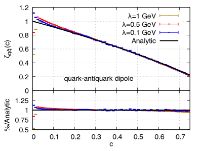
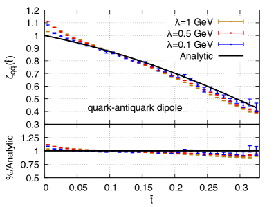
Figure 1: The function $\zeta_{q\bar{q}}(v)$ for the $C$-parameter (left panel) and the thrust $\overline{T}=1-T$ (right panel), evaluated numerically using $q=100$ GeV and $\lambda=0.1,~{}0.5,~{}1$ GeV, compared to the analytic computation (solid line). In the lower panels we reported the ratio plot of each numerical curve with respect to the analytic one.

We start by considering the process $\gamma^{*}(q)\to q(p_{1})+\bar{q}(p_{2})+\gamma(p_{3})$, as in the previous sections. In this case the only emitting dipole is the $q\bar{q}$ system. We then write

$$\delta_{\rm NP}^{q\bar{q}\gamma}=h\zeta_{q\bar{q}}(v),$$ (172)

with $\zeta_{q\bar{q}}(0)=1$ as before. We note that, since for $v=0$ the $q\bar{q}\gamma$ configuration approaches a two-parton $q\bar{q}$ configuration, $h$ must correspond in this case to the non-perturbative shift computed in previous literature for the two-jet configuration. Thus, for the $C$-parameter, we have $h=-(\lambda/q)\alpha_{s}\times 15\pi^{2}/16$, while for the thrust $h=-(\lambda/q)\alpha_{s}\times 5\pi/8$, see eqs. (46) and (147).

In fig. 1 analytic and numerical results Caola:2021kzt are compared for $\zeta_{q\bar{q}}$, for both the $C$-parameter and the thrust. We take $q=100~{}{\rm GeV}$. For the numerical results, we consider three different values of the gluon mass $\lambda=1,~{}0.5,~{}0.1~{}{\rm GeV}$. We observe that the numerical result converges to the analytic one, to a good approximation. However, it is apparent from these figures that the agreement is not perfect and that even smaller values of $\lambda$ should be chosen in numerical computations to improve the situation. Unfortunately, it is quite difficult to do so. This is because the numerical results contain extra quadratic terms in $\lambda$ that can also be enhanced by powers of $\ln\lambda$. We also note that the analytic and numerical results tend to depart from each other at small $v$, for both the $C$-parameter and the thrust. This is because, in this region, the effective hard scale is reduced, so that the expansion parameter for power corrections is no longer $\lambda/q$, but rather $\lambda$ divided by the reduced scale. In contrast, the analytic calculation only contains linear power corrections, and is not affected by these numerical issues.

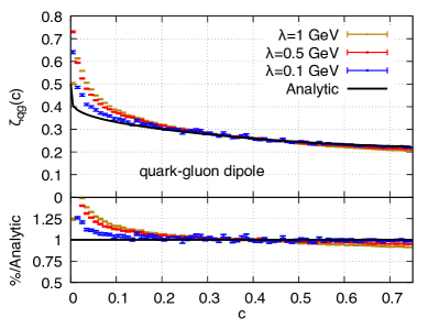
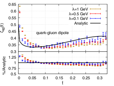
Figure 2: Same as fig. 1, but for the $qg$ dipole.

To generalise the analytic result to the QCD case, $\gamma^{*}(q)\to q(p_{1})+\bar{q}(p_{2})+g(p_{3})$, we consider radiation off the three dipoles $q\bar{q}$, $qg$ and $\bar{q}g$ and account for the relevant color factors, see ref. Caola:2021kzt for more detail. We write

$$\delta_{\rm NP}^{q\bar{q}g}(v)=h\zeta^{q\bar{q}g}(v),~{}~{}~{}~{}~{}~{}~{}~{}~{}~{}~{}\zeta^{q\bar{q}g}(v)=\zeta_{q\bar{q}}(v)\frac{C_{F}-C_{A}/2}{C_{F}}+\zeta_{qg}(v)\frac{C_{A}}{C_{F}},$$ (173)

where we have assumed that the $qg$ and $\bar{q}g$ dipoles contribute equally. In eq. (173), $\zeta_{q\bar{q}}$ is identical to the contribution of the $q\bar{q}$-dipole correction considered in this paper. The function $\zeta_{qg}$ is as $\zeta_{q\bar{q}}$ except that the gluon plays the role of an anti-quark. We note that it follows that $\zeta_{qg}(0)=1/2$ Caola:2021kzt and, hence, $\zeta^{q\bar{q}g}(0)=1$.

In order to get a more realistic prediction, the value of the constant $h$ should be corrected to include also the effects of the gluon splitting into two gluons, as it is commonly done in the dispersive model Dokshitzer:1997iz ; Dokshitzer:1998pt ; Smye:2001gq , but this is irrelevant for us since we only report results for the $\zeta$ function.

We compare analytic and numerical results for $\zeta_{qg}$ in fig. 2. We observe that also in this case the numerical result converges towards the analytic one, and that features discussed in connection with fig. 1 are also present for the $qg$ dipole. We note that it is evident from fig. 2 that the numerical result for the $qg$ dipole is less stable than the result for the $q\bar{q}$ one, so that the availability of the analytic computation in this case is especially welcome.

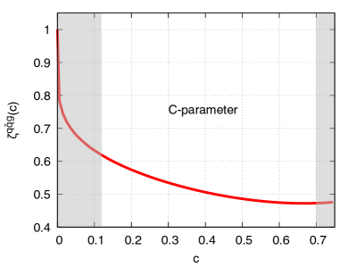
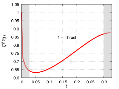
Figure 3: Same as fig. 1, but for the sum of all the dipoles, where each contribution is supplemented with the proper colour factor, as in eq. (173). The grey shading shows the region which is usually excluded from $\alpha_{s}$ determinations Luisoni:2020efy .

6.2 Results for the $C$-parameter and the thrust in the three-jet region and comparison with existing literature

Having validated the analytic result against the numerical ones of ref. Caola:2021kzt , we can compare our predictions to the results in the literature. In fig. 3, we show our prediction for $\zeta^{q\bar{q}g}$ for both the $C$-parameter (left) and the thrust (right) distributions using eq. (173). In those figures the grey shaded areas show the kinematic regions that are typically excluded from high-precision extractions of $\alpha_{s}$ Luisoni:2020efy . We observe that for both the $C$-parameter and the thrust the shape of non-perturbative corrections in the bulk of the three-jet region is non-trivial.

It is interesting to compare our result for the $C$-parameter with the predictions of ref. Luisoni:2020efy . Using eqs. (46, 47), it is straightforward to check that our results agree with those of ref. Luisoni:2020efy at the endpoints $c=0,3/4$. However, in the bulk of the three-jet region the formalism of ref. Luisoni:2020efy does not lead to an unambiguous prediction. Instead, the authors of ref. Luisoni:2020efy adopted an agnostic approach and obtained different results depending on the assumption they made for the recoil due to the emission of a soft massless gluon, see their fig. 3. It is interesting to note that most of the recoil schemes considered in ref. Luisoni:2020efy (Catani-Seymour Catani:1996vz , PanLocal (antenna variant) and PanGlobal Dasgupta:2020fwr ) gave the same result. It turns out that this result is also compatible with our prediction based on eq. (173). The FHP (Forshaw-Holguin-Plätzer) scheme of ref. Forshaw:2020wrq however led to a different prediction.

Our formalism provides a clear explanation of why this is the case. Indeed, the Catani-Seymour, PanLocal, and PanGlobal schemes all satisfy the smoothness requirement in the soft limit that is needed in order for the recoil effects not to contribute to linear power corrections Caola:2021kzt . In other words, if one uses these schemes, then a naive soft analysis leads to the correct result for linear power corrections to the $C$-parameter, without additional contributions. This is not the case for the FHP scheme, which does not satisfy the smoothness requirements. We elaborate on this remark in what follows.

We start by analysing the PanLocal (antenna) mapping. It is dipole-local, which means that it preserves the four-momentum of the radiating dipole. It is defined by

$$p_{1}=\alpha_{1}{\tilde{p}}_{1}+\beta_{1}{\tilde{p}}_{2}-fl_{\perp},\qquad p_{2}=\alpha_{2}{\tilde{p}}_{1}+\beta_{2}{\tilde{p}}_{2}-(1-f)l_{\perp},$$ (174)

where $l$ is the momentum of the radiated soft gluon and $\alpha$ and $\beta$ are specified by the momentum-conservation and on-shell requirements

$$p_{1}+p_{2}+l={\tilde{p}}_{1}+{\tilde{p}}_{2},\qquad\qquad p_{1/2}^{2}=2\alpha_{i}\beta_{i}\,(p_{1}p_{2})+{\cal O}(l_{\perp}^{2})=0\,.$$ (175)

These two equations can be satisfied only if either $\beta_{1}=\alpha_{2}=0$ or $\beta_{2}=\alpha_{1}=0$ up to terms of order $l_{\perp}^{2}$. Assuming the first assignment, eq. (174) implies

$$\alpha_{1}=1-\frac{(l{\tilde{p}}_{2})}{({\tilde{p}}_{1}{\tilde{p}}_{2})}\,,\qquad\qquad\beta_{2}=1-\frac{(l{\tilde{p}}_{1})}{({\tilde{p}}_{1}{\tilde{p}}_{2})}\,,$$ (176)

so, in the soft limit the PanLocal scheme has the form

$$p_{1}=\left(1-\frac{(l{\tilde{p}}_{2})}{({\tilde{p}}_{1}{\tilde{p}}_{2})}\right)\,{\tilde{p}}_{1}-f\,l_{\perp},\qquad p_{2}=\left(1-\frac{(l{\tilde{p}}_{1})}{({\tilde{p}}_{1}{\tilde{p}}_{2})}\right)\,{\tilde{p}}_{2}-(1-f)\,l_{\perp}.$$ (177)

The PanLocal choice for $f$ is

$$f=\frac{e^{2\bar{\eta}_{k}}}{1+e^{2\bar{\eta}_{k}}}\,,$$ (178)

where $\bar{\eta}_{k}$ is a rapidity-type variable, defined as

$$\bar{\eta}_{l}=\frac{1}{2}\ln\frac{(l\tilde{p}_{2})(\tilde{p}_{1}q)}{(l\tilde{p}_{1})(\tilde{p}_{2}q)}.$$ (179)

Thus the PanLocal mapping is non-linear in the soft limit. However, the non linear term is proportional to $l^{\mu}_{\perp}$ with an azimuthally-independent coefficient. Hence, when computing recoil effects using this mapping, the non-linear term always cancels after azimuthal integration, and the PanLocal mapping satisfies the smoothness criteria Caola:2021kzt . The Catani-Seymour mapping is also non-linear, but again the non-linear term vanishes after azimuthal integration for a similar reason.

The PanGlobal mapping is defined as follows. First, one introduces the intermediate variables

$$\bar{p}_{1}=\left(1-\frac{(l{\tilde{p}}_{2})}{({\tilde{p}}_{1}{\tilde{p}}_{2})}\right)\,{\tilde{p}}_{1},\qquad\bar{p}_{2}=\left(1-\frac{(l{\tilde{p}}_{1})}{({\tilde{p}}_{1}{\tilde{p}}_{2})}\right)\,{\tilde{p}}_{2}\,.$$ (180)

Then one finds a boost $B$ followed by a rescaling $R$ to be applied to $\bar{p}_{1},\bar{p}_{2},p_{3}$ such that

$$p_{1/2}=RB\bar{p}_{1/2},\qquad p_{3}=RB{\tilde{p}}_{3},\qquad l^{\prime} =RBl.$$ (181)

In the small-$l$ limit, it is easy to see that this yields the mapping

$$p_{1} \approx{\tilde{p}}_{1}-\frac{({\tilde{p}}_{2}l)}{({\tilde{p}}_{1}{\tilde{p}}_{2})}{\tilde{p}}_{1}-\frac{({\tilde{p}}_{1}q)}{q^{2}}\,l_{\perp}-\frac{(l_{\perp}q)}{q^{2}}\,{\tilde{p}}_{1},$$

$$p_{2} \approx{\tilde{p}}_{2}-\frac{({\tilde{p}}_{1}l)}{({\tilde{p}}_{1}{\tilde{p}}_{2})}{\tilde{p}}_{2}-\frac{({\tilde{p}}_{2}q)}{q^{2}}\,l_{\perp}-\frac{(l_{\perp}q)}{q^{2}}\,{\tilde{p}}_{2},$$ (182)

$$p_{3} \approx{\tilde{p}}_{3}-\frac{({\tilde{p}}_{3}q)}{q^{2}}\,l_{\perp}+\frac{{\tilde{p}}_{3}\cdot l_{\perp}}{q^{2}}\,q-\frac{(l_{\perp}q)}{q^{2}}\,{\tilde{p}}_{3}\,.$$

This is fully linear, and it satisfies the requirements of ref. Caola:2021kzt . As we have said, this implies that with these recoil schemes a naive soft analysis completely captures linear power corrections.

The FHP mapping is similar to the PanGlobal one, but only one side of the dipole is rescaled. In practice, one parametrises the intermediate momenta

$$\bar{p}_{1}=\left(1-\frac{(l{\tilde{p}}_{2})}{({\tilde{p}}_{1}{\tilde{p}}_{2})}\right)\,{\tilde{p}}_{1},\qquad\bar{p}_{2}={\tilde{p}}_{2}\,,$$ (183)

with probability $f(\bar{\eta_{l}})$, where $f$ and $\bar{\eta}_{l}$ are given in eqs. (178) and (179) and coincide with the PanLocal/PanGlobal ones. The parametrisation

$$\bar{p}_{1}={\tilde{p}}_{1},\qquad\bar{p}_{2}=\left(1-\frac{(l{\tilde{p}}_{1})}{({\tilde{p}}_{1}{\tilde{p}}_{2})}\right)\,{\tilde{p}}_{2}\,,$$ (184)

is instead selected with probability $1-f(\bar{\eta_{l}})$. Then the kinematic reconstruction proceeds as in PanGlobal, where all the momenta are rescaled to preserve the mass of the total system, and then boosted in the original event frame. It is thus clear that the soft limit is non-linear in the longitudinal components of the momenta of the radiated parton and, therefore, it does not satisfy the requirements Caola:2021kzt . As a consequence, an analysis of soft emissions is not sufficient to compute the linear power corrections if one were to use this recoil scheme. This is exactly what is seen in fig. 3 of ref. Luisoni:2020efy . We conclude this section by noting that at the endpoints $c=0$, $c=3/4$ all recoil schemes yield the same result. This is expected since in these regions the sensitivity of the shape variable to recoil effects is strongly suppressed Luisoni:2020efy .

7 Conclusions

The goal of this paper was to continue exploration of linear power corrections to shape variables in $e^{+}e^{-}$ annihilation to hadrons that we started in ref. Caola:2021kzt . We performed explicit analytic computations for the $C$-parameter and the thrust distributions and showed that our considerations apply to a large class of shape variables.

Our results can be briefly summarised as follows: linear power corrections which affect cumulants of shape variables in the three-jet region are proportional to a universal, constant factor times a function which characterises the behaviour of the shape variable under the emission of a single soft massless parton. Our result applies a fortiori to the two-jet region where, however, an equivalent result has been formulated long ago Dokshitzer:1998pt .

Our calculations are performed in the large-$n_{f}$ model of QCD, but with a final state $q\bar{q}\gamma$ rather than $q\bar{q}g$. The linear renormalon contribution to shape variables associated with the power correction can be exactly calculated in this framework. It arises from the emission of a soft virtual gluon that can both fluctuate into virtual $q\bar{q}$ pairs and eventually decay into one of them.

Since renormalons can be studied using soft emissions, we can speculate that, in the realistic case of a $q\bar{q}g$ final state, linear power corrections can be obtained by summing up the soft emissions off all three colour dipoles, $q\bar{q}$, $qg$ and $\bar{q}g$, multiplied by the corresponding colour factor. By doing this, we obtain a theoretical prediction that can be confronted with data.

These assumptions are essentially the same ones that underlie the so called dispersive model of power corrections Dokshitzer:1997iz ; Dokshitzer:1998pt . This model is fully consistent with the large-$n_{f}$ limit of QCD, and it was recently applied to the calculation of power corrections to the $C$-parameter near the three-jet symmetric point Luisoni:2020efy .

It is useful to briefly summarise the reasons that allow for the computation of power corrections in the two-jet region, in the three-jet symmetric limit for the $C$-parameter Luisoni:2020efy and in the generic three-jet configuration as described in this paper. In general, we can write the cumulant of a shape variable as

$$\Sigma(v)=\int\mathrm{d}\sigma(\{{\tilde{p}}\})\theta\big{(}V(\{{\tilde{p}}\})-v\big{)}+\int\mathrm{d}\sigma(\{p,k\})\theta\big{(}V(\{p,k\})-v\big{)},$$ (185)

where $\{{\tilde{p}}\}$ denote the hard final state momenta when no soft particles are emitted, $p$ denote the hard momenta in the final state that are accompanied by the emission of a soft gluon, and by $k$ we denote generically the momenta of the final state particles arising from the radiated soft gluon. Furthermore, we assume that $\sigma(\{{\tilde{p}}\})$ also includes the virtual soft gluon corrections, so that the left-hand side of eq. (185) includes all relevant corrections to the cumulant. By $V(\{{\tilde{p}}\})$ and $V(\{p,k\})$ we denote the value of the shape variable computed for the hard partons final state (without soft gluon emission) and for the final state including the gluon emission with its decay products.

In the two-jet region $v\to 0$, the final state consists of two back-to-back partons. Thus $V(\{{\tilde{p}}\})$ is constant, and we can manipulate eq. (185) as follows

$$\Sigma(v) = \left[\int\mathrm{d}\sigma(\{{\tilde{p}}\})+\int\mathrm{d}\sigma(\{p,k\})\right]\theta\big{(}V(\{{\tilde{p}}\})-v\big{)}$$ (186)

$$+ \int\mathrm{d}\sigma(\{p,k\})\left[\theta\big{(}V(\{p,k\})-v\big{)}-\theta\big{(}V(\{{\tilde{p}}\})-v\big{)}\right]\,.$$

We can see now that the first line of eq. (186) is proportional to the total cross section, and thus is free from linear infrared renormalons. In the second term, on the other hand, the factor in the square bracket vanishes in the soft limit, so that the soft approximation to $\mathrm{d}\sigma(\{p,k\})$ is all what is needed for the computation, that can then be carried out along the lines of refs. Dokshitzer:1997iz ; Dokshitzer:1998pt .

If we consider the $C$-parameter near the three-jet symmetric point, the crucial observation is that the contribution to $C$ from the hard partons is given by Luisoni:2020efy

$$C_{\rm hard}=\frac{3}{4}-\frac{81}{16}(\epsilon_{q}^{2}+\epsilon_{q}\epsilon_{\bar{q}}+\epsilon_{\bar{q}}^{2})+{\cal O}(\epsilon^{3}),$$ (187)

where $\epsilon_{q(\bar{q})}=2E_{q(\bar{q})}/E-2/3$ and $E=\sqrt{q^{2}}$ is the total energy. If we apply eq. (185) for $c$ very near $3/4$, the momenta $\{{\tilde{p}}\}$ will be forced to approach the symmetric limit, and $C\{{\tilde{p}}\}$ is nearly constant there. So, we can again carry out the manipulation that led to eq. (186) with $V=C$. Again, the first term is proportional to a cross section that is inclusive in the radiation of the soft gluon, and can be assumed to be free of linear renormalon Caola:2021kzt . Because of eq. (187), we can replace $C(\{p({\tilde{p}},k),k\})-c)\to C(\{{\tilde{p}},k\})-c)$ in the square bracket, and because of the ensuing soft suppression, we can again resort to the soft approximation to perform the computation, as it was done in ref. Luisoni:2020efy . Hence, we see that the derivation in both the two-jet and symmetric three-jet cases discussed above crucially relies on recoil effects being strongly suppressed. As a consequence, it is not immediately clear how to generalise these constructions to the three-jet region beyond the symmetric point.

Let us now see how this problem is solved in this paper. Assuming, for the sake of discussion, that the soft emission originates from a single dipole, we introduce a mapping $p({\tilde{p}},k)$ that, for small $k$, is linear in $k$ and that is collinear-safe when the gluon is collinear to the partons constituting the dipole. Then, for a generic shape variable and for generic momenta we write eq. (185) as

$$\Sigma(v) = \int\big{[}\mathrm{d}\sigma(\{{\tilde{p}}\})+\mathrm{d}\sigma(\{p({\tilde{p}},k),k\})\big{]}\theta\big{(}V(\{{\tilde{p}}\})-v\big{)}$$ (188)

$$+ \int\mathrm{d}\sigma(\{p({\tilde{p}},k),k\})\big{[}\theta\big{(}V(\{p({\tilde{p}},k),k\})-v\big{)}-\theta\big{(}V(\{{\tilde{p}}\})-v\big{)}\big{]}\,.$$

Now the first term involves an inclusive integral of the cross section at fixed underlying Born momenta, with the underlying Born defined by a mapping that is linear in $k$ for small $k$. It was shown in ref. Caola:2021kzt that such integrals do not yield linear power corrections. Hence, we can drop the first line in eq. (188) and consider only the second line, that again can be evaluated in the soft approximation leading to the results discussed in this paper.

Although the phenomenological consequences of our results are yet to be fully explored, we can make a few statements using the results of ref. Luisoni:2020efy . There, in the framework of the dispersive model for power corrections which employs a single non-perturbative parameter related to the low-scale value of the strong coupling constant, several interpolations of the non-perturbative corrections to the $C$-parameter distribution between the two- and three-jet symmetric points were considered, and for each of them a fit of the strong coupling constant was performed. For some of the extrapolations it was found that the fitted value of $\alpha_{s}$ was larger than the one obtained using the conventional assumption that non-perturbative corrections are constant and, therefore, are fixed by their value in the two-jet region. Our results clearly show that the non-perturbative effects in the three-jet region are kinematic-dependent. In fact, our result agrees with the lowest curves in fig. 3 of ref. Luisoni:2020efy that, in turn, are below the line labeled as $\zeta_{b,3}$ there. From table 2 in that reference, we see that the use of $\zeta_{b,3}$ in the $\alpha_{s}$ fit yields the value of $0.1167$ that is larger than the $\alpha_{s}=0.1121$ value obtained by assuming that the non-perturbative coefficient is constant.

In view of these observations, a conservative conclusion from the results of the present paper is that the error on $\alpha_{s}$ determination that employs constant non-perturbative corrections should be considerably enlarged towards the upper side. A more aggressive conclusion would be that the central value should be shifted in the upper direction. However, in the latter case, in view of the fact that several assumptions underlie our findings, chief of which is an Abelian nature of the large-$n_{f}$ calculation, a more refined theoretical understanding and comparison with data should be needed to validate the approach.

Appendix A Renormalon structure of the large-$n_{f}$ result

The exact prediction for the cumulant $\Sigma(v)$ eq. (1) computed in the large-$n_{f}$ approximation reads

$$\Sigma(v)=\Sigma_{\rm b}(v)-\frac{1}{b_{0,f}\alpha_{s}(\mu)}\int_{0}^{\infty}\frac{\mathrm{d}\lambda}{\pi}\frac{\mathrm{d}\Sigma(v;\lambda)}{\mathrm{d}\lambda}\arctan\frac{\pi b_{0,f}\alpha_{s}(\mu)}{1+b_{0,f}\alpha_{s}(\mu)\log\frac{\lambda^{2}e^{-C}}{\mu^{2}}},$$ (189)

where $\Sigma_{\rm b}(v)$ is the LO prediction, $\Sigma(v;\lambda)$ and $b_{0,f}$ are given in eqs. (2, 3) and $C=5/3$. We note that the factor $\alpha_{s}$ in the denominator in front of the integral cancels the factor of $\alpha_{s}$ in $\Sigma(v;\lambda)$. Eq. (189) is well-known (see for example ref. Beneke:1998ui ) as far as the virtual corrections and the inclusive real corrections are concerned, but we are not aware of a reference before FerrarioRavasio:2018ubr where also the $q\bar{q}$ splitting term is cast in the same form. In appendix B of ref. FerrarioRavasio:2018ubr a complete derivation of eq. (189) formula is also given. Examples of real and virtual Feynmann graphs contributing to eq. (189) are illustrated in fig. 4,

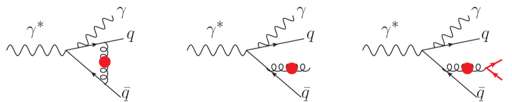
Figure 4: An example of a virtual, a real gluon emission and a real $q\bar{q}$ emission graph contributing to the large-$n_{f}$ correction to the process $\gamma^{*}\to q\bar{q}\gamma$. The right graph, with a $g\to q\bar{q}$ splitting, must be included, since the sum over final state quark flavour leads to a factor of $n_{f}$.

where the solid blob insertion in the gluon propagator represents the inclusion of all corrections given by a fermion loop, as represented by the recursive graphic equation

$$\raisebox{-14.22636pt}{\includegraphics[width=346.89731pt]{figs/bubble_chain}}.$$ (190)

The linear power corrections arise in eq. (189) from the leading term in the small-$\lambda$ expansion of $\Sigma(v;\lambda)$, that leads to

$$\Sigma(v)\approx\Sigma_{b}(v)-\left[\frac{\mathrm{d}\Sigma(v;\lambda)}{\mathrm{d}\lambda}\right]_{\lambda=0}\left\{\frac{1}{b_{0,f}\alpha_{s}(\mu)}\int_{0}^{\mu_{C}}\frac{d\lambda}{\pi}\arctan\frac{\pi b_{0,f}\alpha_{s}(\mu)}{1+b_{0,f}\alpha_{s}(\mu)\log\frac{\lambda^{2}}{\mu_{C}^{2}}}\right\},$$ (191)

where $\mu_{C}=\mu e^{C/2}$. The upper limit of integration is chosen for convenience, since the renormalon structure arises from the region where the denominator in the arctangent vanishes, corresponding to the Landau pole. Thus, any upper limit comprising the Landau pole is acceptable.

The renormalon structure of the expression in the curly bracket of eq. (191), according to the result presented in appendix A of ref. FerrarioRavasio:2020guj , is

$$\begin{split}&\frac{1}{b_{0,f}\alpha_{s}(\mu)}\int_{0}^{\mu_{C}}\frac{d\lambda}{\pi}\arctan\frac{\pi b_{0,f}\alpha_{s}(\mu)}{1+b_{0,f}\alpha_{s}(\mu)\log\frac{\lambda^{2}}{\mu_{C}^{2}}}=\\ &\frac{\mu_{C}}{b_{0,f}\alpha_{s}(\mu)}\left[\text{P}\int_{0}^{\infty}\frac{\mathrm{d}t}{\pi}\frac{\exp\left(-\frac{t}{2b_{0,f}\alpha_{s}(\mu)}\right)}{1-t}+C_{\rm NP}\frac{\Lambda_{\rm QCD}}{\mu}\right]+\mbox{analytic terms in $\alpha_{s}(\mu)$}.\end{split}$$ (192)

In the last term, $\Lambda_{\rm QCD}$ is the QCD (large-$n_{f}$) scale, defined by the equation

$$\alpha_{s}(\mu)=\frac{1}{b_{0,f}\log\frac{\mu^{2}}{\Lambda_{\rm QCD}^{2}}},$$ (193)

so that

$$\exp\left(-\frac{1}{2b_{0,f}\alpha_{s}(\mu)}\right)=\frac{\Lambda_{\rm QCD}}{\mu}.$$ (194)

In ref. FerrarioRavasio:2020guj a further term of the form of eq. (194), arising from the discontinuity of the integrand in eq. (191) at the Landau pole, is added to the principal value part. If a suitable theta function is added to the integrand in (191) such term is not present. The important point, however, is that an ambiguity remains depending upon the handling of the Landau pole. Such ambiguity is related to the residue of the integral at $t=1$, and thus has the form of eq. (194). In eq. (192) we parametrize this ambiguity in terms of an (uncalculable) coefficient $C_{\rm NP}$. We also note that the factorial growth in the asymptotic expansion of the Borel sum in eq. (192) is due to the singularity at $t=1$. Thus its $\mu$ dependence cancels against the $\mu_{C}$ factor, and so does the $\mu$ dependence of the $C_{\rm NP}$ term. See appendix A in ref. FerrarioRavasio:2020guj for more details.

In some phenomenological approaches the expression in the curly bracket of eq. (191) is interpreted as an effective coupling, that in the full theory should be replaced by a QCD effective coupling that also includes non-perturbative effects Dokshitzer:1995qm .

Appendix B The functions $G_{1,..,5}$

The functions $G_{1,..,5}$ were introduced in eq. (28). They read

$$G_{1} =\frac{\left(1-\beta^{2}\right)^{-3/2}}{48\beta^{6}(x(y-1)+1)^{2}(xy-1)^{2}}\Bigg{[}\beta^{6}\Bigg{(}2x^{3}y\left(-42y^{3}+84y^{2}-421y+379\right)$$

$$+29x^{4}(y-1)^{2}y^{2}+x^{2}\left(1706y^{2}-1706y-271\right)+x\left(-948y^{2}+948y+542\right)-271\Bigg{)}$$

$$+\beta^{4}\Bigg{(}-159x^{4}(y-1)^{2}y^{2}+2x^{3}y\left(187y^{3}-374y^{2}+1203y-1016\right)$$

$$+x^{2}\left(-4542y^{2}+4542y+749\right)+2x\left(1255y^{2}-1255y-749\right)+749\Bigg{)}$$ (195)

$$+5\beta^{2}\Bigg{(}47x^{4}(y-1)^{2}y^{2}+2x^{3}y\left(-50y^{3}+100y^{2}-271y+221\right)$$

$$+165x^{2}\left(6y^{2}-6y-1\right)+x\left(-548y^{2}+548y+330\right)-165\Bigg{)}$$

$$-105\Bigg{(}x^{4}(y-1)^{2}y^{2}-2x^{3}y\left(y^{3}-2y^{2}+5y-4\right)+3x^{2}\left(6y^{2}-6y-1\right)$$

$$+x\left(-10y^{2}+10y+6\right)-3\Bigg{)}\Bigg{]},$$

$$G_{2} =\frac{\sqrt{1-\beta^{2}}(x-1)\ln^{2}\left(\frac{1+\beta}{1-\beta}\right)}{32\beta^{8}x(x(y-1)+1)^{2}(xy-1)^{2}}$$

$$\times\Bigg{[}\beta^{4}\left(x^{2}\left(-117y^{2}+117y+34\right)+83x^{3}(y-1)y-53x+19\right)$$ (196)

$$-10\beta^{2}\left(x^{2}\left(-29y^{2}+29y+8\right)+21x^{3}(y-1)y-11x+3\right)$$

$$+35\left(x^{2}\left(-7y^{2}+7y+2\right)+5x^{3}(y-1)y-3x+1\right)\Bigg{]},$$

$$G_{3} =\frac{\ln\left(\frac{\sqrt{1-\beta^{2}c_{12}^{2}}+\beta s_{12}}{\sqrt{1-\beta^{2}c_{12}^{2}}-\beta s_{12}}\right)}{96\beta^{7}\left(1-\beta^{2}\right)^{3/2}s_{12}x\sqrt{1-\beta^{2}c_{12}^{2}}(x(y-1)+1)(xy-1)}$$

$$\times\Bigg{[}\beta^{8}x\left(29x^{2}(y-1)y+x\left(-84y^{2}+84y+15\right)-15\right)$$

$$-2\beta^{6}\left(x^{2}\left(-229y^{2}+229y+51\right)+94x^{3}(y-1)y-186x+135\right)$$ (197)

$$+\beta^{4}\left(x^{2}\left(-874y^{2}+874y+232\right)+394x^{3}(y-1)y-758x+526\right)$$

$$-10\beta^{2}\left(x^{2}\left(-71y^{2}+71y+25\right)+34x^{3}(y-1)y-78x+53\right)$$

$$+105(x-2)\left(x^{2}(y-1)y+x-1\right)\Bigg{]},$$

$$G_{4} =\frac{\ln\left(\frac{1+\beta}{1-\beta}\right)}{96\beta^{7}\left(1-\beta^{2}\right)^{3/2}x(x(y-1)+1)^{2}(xy-1)^{2}}\Bigg{[}\beta^{8}x\Bigg{(}3x^{4}(y-1)^{2}y^{2}$$

$$-6x^{3}y\left(2y^{3}-4y^{2}+57y-55\right)+x^{2}\left(758y^{2}-758y-113\right)$$

$$+x\left(-428y^{2}+428y+226\right)-113\Bigg{)}-6\beta^{6}\Bigg{(}11x^{5}(y-1)^{2}y^{2}$$

$$+x^{4}y\left(-29y^{3}+58y^{2}-479y+450\right)+x^{3}\left(1046y^{2}-1046y-171\right)$$ (198)

$$+x^{2}\left(-596y^{2}+596y+387\right)-261x+45\Bigg{)}+2\beta^{4}\Bigg{(}114x^{5}(y-1)^{2}y^{2}$$

$$+x^{4}y\left(-261y^{3}+522y^{2}-3187y+2926\right)+8x^{3}\left(848y^{2}-848y-139\right)$$

$$+x^{2}\left(-3858y^{2}+3858y+2487\right)-1638x+263\Bigg{)}-10\beta^{2}\Bigg{(}27x^{5}(y-1)^{2}y^{2}$$

$$+x^{4}y\left(-57y^{3}+114y^{2}-607y+550\right)+x^{3}\left(1278y^{2}-1278y-211\right)$$

$$+x^{2}\left(-728y^{2}+728y+475\right)-317x+53\Bigg{)}+105\Big{(}x^{5}(y-1)^{2}y^{2}$$

$$-2x^{4}y\left(y^{3}-2y^{2}+10y-9\right)+7x^{3}\left(6y^{2}-6y-1\right)-8x^{2}\left(3y^{2}-3y-2\right)-11x+2\Big{)}\Bigg{]},$$

$$G_{5} =\frac{\sqrt{1-\beta^{2}}\ln\left(\frac{1+\beta}{1-\beta}\right)\ln\left(\frac{\sqrt{1-\beta^{2}c_{12}^{2}}+\beta s_{12}}{\sqrt{1-\beta^{2}c_{12}^{2}}-\beta s_{12}}\right)}{64\beta^{8}s_{12}x(x(y-1)+1)(xy-1)\sqrt{1-\beta^{2}c_{12}^{2}}}$$

$$\times\Bigg{[}\beta^{6}x\left(x^{2}(y-1)y+x\left(-4y^{2}+4y-5\right)+5\right)+\beta^{4}\Bigg{(}x^{2}\left(54y^{2}-54y-17\right)$$

$$-21x^{3}(y-1)y+55x-38\Bigg{)}+5\beta^{2}\Bigg{(}x^{2}\left(-24y^{2}+24y+5\right)$$ (199)

$$+11x^{3}(y-1)y-17x+12\Bigg{)}-35(x-2)\left(x^{2}(y-1)y+x-1\right)\Bigg{]}.$$

Appendix C Elliptic integration

The goal of the discussion in this appendix is to explain how the integrals in eq. (28) can be calculated in a systematic way using state-of-the-art technology. First, in appendix C.1 we will show how the integration can be recast so that the elliptic multiple polylogarithms Broedel:2017kkb ; Broedel:2017siw appear naturally. This will allow us to obtain an analytic expression for $I_{i}$ in eq. (28), albeit a quite complicated one. To simplify it, in appendix C.2 we will express it in terms of the so-called $\tilde{\Gamma}$ integrals (see refs. Broedel:2017kkb ; Broedel:2017siw ; Broedel:2018iwv ; Broedel:2018qkq ; Broedel:2019hyg ; Weinzierl:2022eaz ) and note that for the purposes of our calculation we only require kernels evaluated at special, rational points. This will allow us to rewrite our result in terms of iterated Eisenstein integrals, and observe a significant simplification in the final expression. In this appendix, we will assume that the reader is familiar with the elliptic polylogarithms literature. For convenience, we will provide a minimal background necessary to follow the relevant steps in appendix D.

C.1 Set-up of the calculation and result in terms of MPLs and eMPLs

The functions $G_{1,..,5}$ displayed in appendix B contain the integration variable $\beta$ under the square roots $\sqrt{1-\beta^{2}}$ and $\sqrt{1-\beta^{2}c_{12}^{2}}$. In particular, $G_{1,2,4}$ only contains the first square root, while $G_{3,5}$ contain both. We consider the integration of $G_{1,2,4}$ first.

To rewrite the integrand in a form suitable for the integration with multiple polylogarithmic kernels, we rationalise the square root with a variable transformation Besier:2018jen ; Besier:2019kco

$$\beta=\frac{2z}{1+z^{2}},$$ (200)

so that

$${\rm d}\beta=\frac{2\left(1-z^{2}\right)}{\left(1+z^{2}\right)^{2}}\;{\rm d}z.$$ (201)

The new integration limits are

$$0<z<\sqrt{\frac{\omega_{\rm max}-\lambda}{\omega_{\rm max}+\lambda}}.$$ (202)

We note that each integral

$$I_{i}=\int\limits_{0}^{\beta_{\rm max}}{\rm d}\beta\,G_{i},\;\;\;i=1,..,5,$$ (203)

is divergent at $\beta=0$ but their sum is finite. Since we will compute all the different integrals separately, we will need to introduce a lower integration boundary $\beta_{\rm min}$. This implies that the lower integration boundary for the variable $z$ is

$$z_{\rm min}=\frac{\beta_{\rm min}}{1+\sqrt{1-\beta_{\rm min}^{2}}}.$$ (204)

We note that care has to be taken that the expansion in $z_{\rm min}$ is done properly for each individual expression up to finite terms. Similarly, as we are interested only in ${\cal O}(\lambda)$ contribution to the $C$-parameter, we need to compute each term $G_{i}$ only up to $\mathcal{O}{\left(\lambda^{0}\right)}$ since we already have a global factor $\lambda/q$ in front of the integral in eq. (28). The change of variable in eq. (200) allows us to express the result for $I_{1,2,4}$ in terms of the multiple polylogarithmic functions (MPLs) of ref. Goncharov:1998kja ; Goncharov:2001iea . After expanding around $\beta_{\rm min}=0$ and $\lambda=0$, we obtain

$$I_{1}= -\frac{\omega_{\rm max}}{\lambda}\frac{2(x-1)\left(3x^{2}(y-1)y+x\left(-4y^{2}+4y+1\right)-1\right)}{3(x(y-1)+1)^{2}(xy-1)^{2}}$$

$$-\frac{1}{\beta_{\rm min}^{5}}\frac{7}{16(x(y-1)+1)^{2}(xy-1)^{2}}\left[x^{4}(y-1)^{2}y^{2}-2x^{3}y\left(y^{3}-2y^{2}+5y-4\right)\right.$$

$$\left.+3x^{2}\left(6y^{2}-6y-1\right)+x\left(-10y^{2}+10y+6\right)-3\right]$$

$$+\frac{1}{\beta_{\rm min}^{3}}\frac{5}{288(x(y-1)+1)^{2}(xy-1)^{2}}\left[31x^{4}(y-1)^{2}y^{2}+2x^{3}y\left(-37y^{3}+74y^{2}\right.\right.$$ (205)

$$\left.\left.-227y+190\right)+141x^{2}\left(6y^{2}-6y-1\right)+x\left(-466y^{2}+466y+282\right)-141\right]$$

$$-\frac{1}{\beta_{\rm min}}\frac{1}{384(x(y-1)+1)^{2}(xy-1)^{2}}\left[27x^{4}(y-1)^{2}y^{2}+2x^{3}y\left(-71y^{3}+142y^{2}\right.\right.$$

$$\left.-1239y+1168\right)+x^{2}\left(5286y^{2}-5286y-817\right)$$

$$\left.+x\left(-2950y^{2}+2950y+1634\right)-817\right],$$

$$I_{2}= \frac{1}{\beta_{\rm min}^{5}}\frac{7(x-1)\left(5x^{3}(y-1)y+x^{2}\left(-7y^{2}+7y+2\right)-3x+1\right)}{8x(x(y-1)+1)^{2}(xy-1)^{2}}$$

$$-\frac{1}{\beta_{\rm min}^{3}}\frac{5\left((x-1)\left(217x^{3}(y-1)y+x^{2}\left(-299y^{2}+299y+82\right)-111x+29\right)\right)}{144\left(x(x(y-1)+1)^{2}(xy-1)^{2}\right)}$$

$$+\frac{1}{\beta_{\rm min}}\frac{(x-1)\left(4121x^{3}(y^{2}-y)-x^{2}\left(5875(y^{2}-y)-1754\right)-2895x+1141\right)}{576x(x(y-1)+1)^{2}(xy-1)^{2}}$$ (206)

$$-\frac{\pi^{2}(x-1)\left(85x^{3}(y-1)y+x^{2}\left(-127y^{2}+127y+42\right)-83x+41\right)}{256\left(x(x(y-1)+1)^{2}(xy-1)^{2}\right)},$$

$$I_{4}= \frac{1}{\beta_{\rm min}^{5}}\frac{7}{16x(x(y-1)+1)^{2}(xy-1)^{2}}\left[x^{5}(y-1)^{2}y^{2}-2x^{4}y\left(y^{3}-2y^{2}+10y-9\right)\right.$$

$$\left.+7x^{3}\left(6y^{2}-6y-1\right)-8x^{2}\left(3y^{2}-3y-2\right)-11x+2\right]$$

$$-\frac{1}{\beta_{\rm min}^{3}}\frac{5}{288\left(x(x(y-1)+1)^{2}(xy-1)^{2}\right)}\left[31x^{5}(y-1)^{2}y^{2}-74x^{4}y\left(y^{2}(y-2)\right.\right.$$

$$\left.\left.+12y-11\right)+x^{3}\left(1878(y^{2}-y)-305\right)-x^{2}\left(1064(y^{2}-y)-668\right)-421x+58\right]$$

$$+\frac{1}{\beta_{\rm min}}\frac{1}{1152x(x(y-1)+1)^{2}(xy-1)^{2}}\left[81x^{5}(y-1)^{2}y^{2}-2x^{4}y\left(213y^{2}(y-2)\right.\right.$$ (207)

$$\left.+7838y-7625\right)+x^{3}\left(35850(y^{2}-y)-5959\right)-200x^{2}\left(103(y^{2}-y)-71\right)$$

$$\left.-10523x+2282\right]$$

$$+\frac{\omega_{\rm max}}{\lambda}\frac{4(1-x)\left((2x^{3}-3x^{2})(y^{2}-y)+(1-x)^{2}\right)(\log{\frac{\lambda}{2\omega_{\rm max}}}+1)}{3x(xy-1)^{2}(xy-x+1)^{2}}$$

$$-\frac{\pi^{2}}{1024x(xy-1)^{2}(xy-x+1)^{2}}\left[3x^{5}y^{2}(1-y)^{2}-2x^{4}y^{3}(y-2)-536x^{4}y^{2}\right.$$

$$\left.+534x^{4}y+(1278x^{3}-744x^{2})(y^{2}-y)-205x^{3}+492x^{2}-369x+82\right].$$

We now turn to the discussion of $I_{3,5}$. These cannot be written in terms of MPLs since the corresponding integrands $G_{3,5}$ involve the second square root $\sqrt{1-c_{12}^{2}\beta^{2}}$. To deal with this case, we find it convenient to introduce another variable transformation, namely

$$\beta=\frac{2\tilde{z}}{\left(1+s_{12}\right)+\left(1-s_{12}\right)\tilde{z}^{2}},~{}~{}~{}~{}~{}~{}\tilde{z}\in(0,1).$$ (208)

With this transformation, the second square root rationalises

$$\sqrt{1-c_{12}^{2}\beta^{2}}=\frac{\left(1+s_{12}\right)-\left(1-s_{12}\right)\tilde{z}^{2}}{\left(1+s_{12}\right)+\left(1-s_{12}\right)\tilde{z}^{2}}\,,$$ (209)

while the quadratic term under the first one turns into a quartic polynomial in $\tilde{z}$

$$\sqrt{1-\beta^{2}}=\frac{1-s_{12}}{\left(1+s_{12}\right)+\left(1-s_{12}\right)\tilde{z}^{2}}\times\sqrt{(\tilde{z}-q_{1})(\tilde{z}-q_{2})(\tilde{z}-q_{3})(\tilde{z}-q_{4})}.$$ (210)

The branch points read

$$q_{1}=-\frac{1+s_{12}}{1-s_{12}},\;\;\;\;\;\;q_{2}=-1,\;\;\;\;\;\;q_{3}=1,\;\;\;\;\;\;q_{4}=\frac{1+s_{12}}{1-s_{12}}.$$ (211)

Integrals containing a square root of a degree four polynomial can be written in terms of elliptic multiple polylogarithms (eMPLs) Broedel:2017kkb ; Broedel:2017siw , see appendix D.1 for a quick review. We obtain

$$I_{3}= \frac{1}{\beta_{\rm min}^{5}}\frac{7(x-2)}{16x}-\frac{1}{\beta_{\rm min}^{3}}\frac{5\left(31x^{3}y^{2}-31x^{3}y-74x^{2}y^{2}+74x^{2}y+23x^{2}-81x+58\right)}{288(x(xy-1)(xy-x+1))}$$

$$+\frac{1}{\beta_{\rm min}}\frac{1}{1152x(x(y-1)+1)^{2}(xy-1)^{2}}\left[81x^{5}(y-1)^{2}y^{2}+2x^{4}y\left(-213y^{3}+426y^{2}\right.\right.$$

$$\left.\left.+404y-617\right)+x^{3}\left(-4134y^{2}+4134y+1057\right)+4x^{2}\left(725y^{2}-725y-1099\right)\right.$$

$$\left.+5621x-2282\right]+\frac{\omega_{\rm max}}{\lambda}\frac{4}{3x}\left[\log{s_{12}}-\log{\frac{\lambda}{2\omega_{\rm max}}}-1\right]$$ (212)

$$+\frac{(x-1)^{2}}{512s_{12}x(xy-1)^{3}(xy-x+1)^{3}}\left(160x^{4}y^{4}-320x^{4}y^{3}+160x^{4}y^{2}+192x^{3}y^{2}\right.$$

$$\left.-192x^{3}y-68x^{2}y^{2}+68x^{2}y+37x^{2}+45x-82\right)\left\{\frac{\pi^{2}}{4}+\operatorname{G}{\left(0,\frac{s_{12}+1}{1-s_{12}},1\right)}\right.$$

$$-\operatorname{G}{\left(0,\frac{s_{12}+1}{s_{12}-1},1\right)}+\operatorname{E}_{4}{\left(\begin{smallmatrix}-1&1\\ \infty&\frac{s_{12}+1}{1-s_{12}}\end{smallmatrix};1,\vec{q}\right)}-\operatorname{E}_{4}{\left(\begin{smallmatrix}-1&1\\ \infty&\frac{s_{12}+1}{s_{12}-1}\end{smallmatrix};1,\vec{q}\right)}$$

$$+\operatorname{E}_{4}{\left(\begin{smallmatrix}-1&1\\ 0&\frac{s_{12}+1}{1-s_{12}}\end{smallmatrix};1,\vec{q}\right)}-\operatorname{E}_{4}{\left(\begin{smallmatrix}-1&1\\ 0&\frac{s_{12}+1}{s_{12}-1}\end{smallmatrix};1,\vec{q}\right)}+\operatorname{E}_{4}{\left(\begin{smallmatrix}-1&1\\ \infty&-1\end{smallmatrix};1,\vec{q}\right)}$$

$$\left.-\operatorname{E}_{4}{\left(\begin{smallmatrix}-1&1\\ \infty&1\end{smallmatrix};1,\vec{q}\right)}+\operatorname{E}_{4}{\left(\begin{smallmatrix}-1&1\\ 0&-1\end{smallmatrix};1,\vec{q}\right)}-\operatorname{E}_{4}{\left(\begin{smallmatrix}-1&1\\ 0&1\end{smallmatrix};1,\vec{q}\right)}\right\},$$

and

$$I_{5}= -\frac{1}{\beta_{\rm min}^{5}}\frac{7(x-2)}{16x}+\frac{1}{\beta_{\rm min}^{3}}\frac{5\left(31x^{3}(y-1)y+x^{2}\left(-74y^{2}+74y+23\right)-81x+58\right)}{288x(x(y-1)+1)(xy-1)}$$

$$+\frac{1}{\beta_{\rm min}}\frac{1}{1152x(x(y-1)+1)^{2}(xy-1)^{2}}\left[-81x^{5}(y-1)^{2}y^{2}+2x^{4}y\left(213y^{3}-426y^{2}\right.\right.$$

$$\left.\left.-404y+617\right)+x^{3}\left(4134y^{2}-4134y-1057\right)+x^{2}\left(-2900y^{2}+2900y+4396\right)\right.$$

$$\left.-5621x+2282\right]-\frac{\pi^{2}(x-1)^{2}}{1024s_{12}x(x(y-1)+1)^{3}(xy-1)^{3}}\times$$

$$\times\left(160x^{4}(y-1)^{2}y^{2}+192x^{3}(y-1)y+x^{2}\left(-68y^{2}+68y+37\right)+45x-82\right)$$

$$+\frac{1}{1024x(xy-1)^{2}(xy-x+1)^{2}}\left[3x^{5}y^{4}-6x^{5}y^{3}+3x^{5}y^{2}-2x^{4}y^{4}+4x^{4}y^{3}-196x^{4}y^{2}\right.$$

$$\left.+194x^{4}y+430x^{3}y^{2}-430x^{3}y-37x^{3}-236x^{2}y^{2}+236x^{2}y-8x^{2}+127x-82\right]\times$$

$$\times\left[-4\operatorname{E}_{4}{\left(\begin{smallmatrix}-1&1\\ 0&\frac{1+s_{12}}{1-s_{12}}\end{smallmatrix};1,\vec{q}\right)}+4\operatorname{E}_{4}{\left(\begin{smallmatrix}-1&1\\ 0&\frac{1+s_{12}}{-1+s_{12}}\end{smallmatrix};1,\vec{q}\right)}-4\operatorname{G}{\left(0,\frac{s_{12}+1}{1-s_{12}};1\right)}\right.$$

$$\left.+4\operatorname{G}{\left(0,\frac{s_{12}+1}{s_{12}-1};1\right)}+\pi^{2}\right]+\operatorname{E}_{4}{\left(\begin{smallmatrix}0\\ 0\end{smallmatrix};1,\vec{q}\right)}\left[\frac{5\pi^{2}(x-1)^{2}\left(x^{2}(y-1)y+1\right)}{8s_{12}x(x(y-1)+1)^{2}(xy-1)^{2}}\frac{\eta_{1}}{\omega_{1}}\right.$$

$$\left.+\frac{5\pi^{2}(x-1)^{2}\left(2x^{4}(y-1)^{2}y^{2}+7x^{3}(y-1)y+x^{2}\left(-8y^{2}+8y+3\right)-5x+2\right)}{96s_{12}x(x(y-1)+1)^{3}(xy-1)^{3}}\right]$$

$$+\left(\frac{5(x-1)^{2}\left(x^{2}(y-1)y+1\right)}{8s_{12}x(x(y-1)+1)^{2}(xy-1)^{2}}+\frac{5(x-1)^{2}\left(x^{2}(y-1)y+1\right)}{8x(x(y-1)+1)^{2}(xy-1)^{2}}\right)\operatorname{E}_{4}{\left(\begin{smallmatrix}-1&1\\ \infty&\frac{s_{12}+1}{1-s_{12}}\end{smallmatrix};1,\vec{q}\right)}$$

$$+\left(-\frac{5(x-1)^{2}\left(x^{2}(y-1)y+1\right)}{8s_{12}x(x(y-1)+1)^{2}(xy-1)^{2}}-\frac{5(x-1)^{2}\left(x^{2}(y-1)y+1\right)}{8x(x(y-1)+1)^{2}(xy-1)^{2}}\right)\times$$

$$\times\operatorname{E}_{4}{\left(\begin{smallmatrix}-1&1\\ \infty&\frac{s_{12}+1}{s_{12}-1}\end{smallmatrix};1,\vec{q}\right)}+\left(\frac{5(x-1)^{2}\left(x^{2}(y-1)y+1\right)}{8s_{12}x(x(y-1)+1)^{2}(xy-1)^{2}}\right.$$

$$\left.+\frac{-3x^{3}(y-1)y+x^{2}\left(2y^{2}-2y+37\right)-115x+78}{256x(x(y-1)+1)(xy-1)}\right)\operatorname{E}_{4}{\left(\begin{smallmatrix}-1&1\\ \infty&-1\end{smallmatrix};1,\vec{q}\right)}$$

$$+\operatorname{E}_{4}{\left(\begin{smallmatrix}-1&1\\ \infty&1\end{smallmatrix};1,\vec{q}\right)}\left(\frac{3x^{3}(y-1)y+x^{2}\left(-2y^{2}+2y-37\right)+115x-78}{256x(x(y-1)+1)(xy-1)}\right.$$ (213)

$$\left.-\frac{5(x-1)^{2}\left(x^{2}(y-1)y+1\right)}{8s_{12}x(x(y-1)+1)^{2}(xy-1)^{2}}\right)+\frac{5(x-1)^{2}\left(x^{2}y^{2}-x^{2}y+1\right)}{16s_{12}x(xy-1)^{2}(xy-x+1)^{2}}\times$$

$$\times\left[-\operatorname{E}_{4}{\left(\begin{smallmatrix}2&1\\ \frac{s_{12}+1}{1-s_{12}}&\frac{s_{12}+1}{1-s_{12}}\end{smallmatrix};1,\vec{q}\right)}+\operatorname{E}_{4}{\left(\begin{smallmatrix}2&1\\ \frac{s_{12}+1}{1-s_{12}}&\frac{s_{12}+1}{s_{12}-1}\end{smallmatrix};1,\vec{q}\right)}+\operatorname{E}_{4}{\left(\begin{smallmatrix}2&1\\ \frac{s_{12}+1}{s_{12}-1}&\frac{s_{12}+1}{1-s_{12}}\end{smallmatrix};1,\vec{q}\right)}\right.$$

$$-\operatorname{E}_{4}{\left(\begin{smallmatrix}2&1\\ \frac{s_{12}+1}{s_{12}-1}&\frac{s_{12}+1}{s_{12}-1}\end{smallmatrix};1,\vec{q}\right)}+\operatorname{E}_{4}{\left(\begin{smallmatrix}2&1\\ -1&-1\end{smallmatrix};1,\vec{q}\right)}-\operatorname{E}_{4}{\left(\begin{smallmatrix}2&1\\ -1&1\end{smallmatrix};1,\vec{q}\right)}-\operatorname{E}_{4}{\left(\begin{smallmatrix}2&1\\ 1&-1\end{smallmatrix};1,\vec{q}\right)}$$

$$+\operatorname{E}_{4}{\left(\begin{smallmatrix}2&1\\ 1&1\end{smallmatrix};1,\vec{q}\right)}+Z_{4}{\left(1\right)}\left(\operatorname{G}{\left(\frac{s_{12}+1}{s_{12}-1},\frac{s_{12}+1}{s_{12}-1};1\right)}+\operatorname{G}{\left(\frac{s_{12}+1}{1-s_{12}},\frac{s_{12}+1}{1-s_{12}};1\right)}-\frac{\pi^{2}}{12}\right.$$

$$-\operatorname{G}{\left(\frac{s_{12}+1}{1-s_{12}},\frac{s_{12}+1}{s_{12}-1},1\right)}-\operatorname{G}{\left(\frac{s_{12}+1}{s_{12}-1},\frac{s_{12}+1}{1-s_{12}};1\right)}+\operatorname{E}_{4}{\left(\begin{smallmatrix}1&1\\ 1&-1\end{smallmatrix};1,\vec{q}\right)}$$

$$\left.\left.-\operatorname{E}_{4}{\left(\begin{smallmatrix}1&1\\ 1&1\end{smallmatrix};1,\vec{q}\right)}\right)\right],$$

where $Z_{4}$, $\omega_{1}$ and $\eta_{1}$ are defined for a generic elliptic curve in eqs. (236, 239, 241). In our case they read

$$Z_{4}(1)=\frac{2\pi i}{\omega_{1}},~{}~{}~{}~{}~{}\omega_{1}=2K(c_{12}^{2}),~{}~{}~{}~{}~{}\eta_{1}=E(c_{12}^{2})-\frac{1+s_{12}^{2}}{3}K(c_{12}^{2}),$$ (214)

where $K$ and $E$ are the complete elliptic integrals of the first and second kind, see eq. (42).

Combining the five contributions eqs. (C.1, C.1, C.1, C.1, C.1), we observe that terms that are singular in the limit $\beta_{\rm min}\to 0$ cancel out so that this limit can be taken safely. Unfortunately, apart from this, no significant simplifications are observed and we are left with a complicated linear combination of elliptic multiple polylogarithms $\operatorname{E}_{4}$.

C.2 Result in terms of Eisenstein integrals

To proceed further, we rewrite the result of the previous section in terms of the so-called $\tilde{\Gamma}$ iterated integrals

$$\tilde{\Gamma}{\left(\begin{smallmatrix}n_{1}&...&n_{m}\\ z_{1}&...&z_{m}\end{smallmatrix};z,\tau\right)}=\int\limits_{0}^{z}dz^{\prime}g^{\left(n_{1}\right)}{\left(z^{\prime}-z_{1},\tau\right)}\tilde{\Gamma}{\left(\begin{smallmatrix}n_{2}&...&n_{m}\\ z_{2}&...&z_{m}\end{smallmatrix};z^{\prime},\tau\right)},$$ (215)

see refs. Broedel:2017kkb ; Broedel:2017siw ; Broedel:2018iwv ; Broedel:2018qkq ; Broedel:2019hyg ; Weinzierl:2022eaz for details and appendix D.2 for a quick overview. Here, $\tau$ is the ratio of the periods of the torus associated with the elliptic curve – see eq. (247) – and the $g^{(n)}$ functions are integration kernels whose exact form is irrelevant for our discussion. What is important is that in our case the kernels only have to be evaluated at specific, rational points. Indeed, upon inspection we find that in our calculation we only need to consider the origin and three half periods

$$z_{q_{1}}=0,\hskip 28.45274ptz_{q_{2}}=\frac{\tau}{2},\hskip 28.45274ptz_{q_{3}}=\frac{\tau}{2}+\frac{1}{2},\hskip 28.45274ptz_{q_{4}}=\frac{1}{2},$$ (216)

as well as three additional points

$$z_{0}=\frac{1}{4}+\frac{\tau}{2},\hskip 28.45274ptz_{\infty}=\frac{1}{4},\hskip 28.45274ptz_{-\infty}=\frac{1}{4}.$$ (217)

Because of this, major simplifications happen. Indeed, the full result can be written as an integral of modular forms and can be expressed in terms of the so-called iterated Eisenstein integrals

$$I{\left(f_{1},...,f_{n};\tau\right)}=\int\limits_{i\infty}^{\tau}\frac{d\tau^{\prime}}{2\pi i}f_{1}{\left(\tau^{\prime}\right)}I{\left(f_{2},...,f_{n};\tau^{\prime}\right)},$$ (218)

see refs. Adams:2017ejb ; Broedel:2018iwv ; Abreu:2019fgk ; Duhr:2019rrs ; Weinzierl:2022eaz ; Abreu:2022vei for details and appendix D.2 for a brief review. In terms of these functions, we can write our result for the linear $\lambda$ term of $I_{C}$ in eq. (27) as

$$\mathcal{T}_{\lambda}\left[I_{C}\right]=-\frac{3}{4\pi^{3}}\frac{\lambda}{q}(t_{1}+t_{2}+t_{3}),$$ (219)

with

$$t_{1}= \frac{5(x-1)^{2}\left(x^{2}(y-1)y+1\right)}{4\pi^{2}\omega_{1}s_{12}x(x(y-1)+1)^{2}(xy-1)^{2}}\times$$

$$\times\left[I{\left(1,h^{(3)}_{4,1,2},\tau\right)}\left(-2\omega_{1}(s_{12}+1)g^{\left(1\right)}{\left(\frac{1}{4},\tau\right)}-g^{\left(2\right)}{\left(\frac{3}{4},\tau\right)}\right.\right.$$

$$\left.\hskip 17.07182pt+g^{\left(2\right)}{\left(-\frac{1}{4},\tau\right)}+\omega_{1}^{2}(s_{12}+1)^{2}\right)$$ (220)

$$\hskip 17.07182pt+i\pi I{\left(h^{(3)}_{4,1,0},\tau\right)}\left(-g^{\left(1\right)}{\left(\frac{1}{4},\tau\right)}+g^{\left(1\right)}{\left(\frac{3}{4},\tau\right)}+\omega_{1}s_{12}+\omega_{1}\right)$$

$$\hskip 17.07182pt\left.+i\pi I{\left(h^{(3)}_{4,1,2},\tau\right)}\left(g^{\left(1\right)}{\left(\frac{\tau}{2}+\frac{1}{4},\tau\right)}-g^{\left(1\right)}{\left(\frac{\tau}{2}+\frac{3}{4},\tau\right)}+\omega_{1}(s_{12}-1)\right)\right],$$

$$t_{2}= \frac{1}{384\pi s_{12}x\left(x^{2}(y-1)y+x-1\right)^{3}}\times$$

$$\times\left[-\frac{6\tilde{C}(x(y-1)+1)(xy-1)}{\omega_{1}}\left(\omega_{1}g^{\left(1\right)}{\left(\frac{1}{4},\tau\right)}\left(s_{12}(x(y-1)+1)(xy-1)\times\right.\right.\right.$$

$$\left.\times(x(x((3x-2)(y-1)y-37)+115)-78)-160(x-1)^{2}\left(x^{2}(y-1)y+1\right)\right)$$

$$\left.+80(x-1)^{2}\left(x^{2}(y-1)y+1\right)\left(g^{\left(2\right)}{\left(\frac{\tau}{2}-\frac{1}{4},\tau\right)}-g^{\left(2\right)}{\left(\frac{\tau}{2}+\frac{3}{4},\tau\right)}\right)\right)$$ (221)

$$+3\tilde{C}\omega_{1}(s_{12}+1)(x(y-1)+1)(xy-1)\left(s_{12}(x(y-1)+1)(xy-1)\times\right.$$

$$\left.\times(x(x((3x-2)(y-1)y-37)+115)-78)-160(x-1)^{2}\left(x^{2}(y-1)y+1\right)\right)$$

$$+5\pi^{3}(x-1)^{2}\left(12\eta_{1}(x(y-1)+1)(xy-1)\left(x^{2}(y-1)y+1\right)\right.$$

$$\left.\left.+\omega_{1}(x(x((y-1)y(x(2x(y-1)y+7)-8)+3)-5)+2)\right)\right],$$

$$t_{3}= -\frac{1}{128\pi^{2}\omega_{1}s_{12}x\left(x^{2}(y-1)y+x-1\right)^{2}}I{\left(1,h^{(3)}_{4,1,0},\tau\right)}\times$$

$$\times\left[2\omega_{1}g^{\left(1\right)}{\left(\frac{1}{4},\tau\right)}\left(s_{12}(x(y-1)+1)(xy-1)(x(x((3x-2)(y-1)y-37)\right.\right.$$

$$\left.+115)-78)\right)-160(x-1)^{2}\left(x^{2}(y-1)y+1\right)\times$$ (222)

$$\times\left(2\omega_{1}g^{\left(1\right)}{\left(\frac{1}{4},\tau\right)}+g^{\left(2\right)}{\left(\frac{\tau}{2}+\frac{3}{4},\tau\right)}-g^{\left(2\right)}{\left(\frac{\tau}{2}-\frac{1}{4},\tau\right)}\right)$$

$$+\omega_{1}^{2}(s_{12}+1)\left(160(x-1)^{2}\left(x^{2}(y-1)y+1\right)\right.$$

$$\left.\left.-s_{12}(x(y-1)+1)(xy-1)(x(x((3x-2)(y-1)y-37)+115)-78)\right)\right].$$

In these equations, $h^{(n)}_{N,r,s}$ are specific kernels of the iterated integrals (labeled generically $f_{1}$ in eq. (218), see appendix D.2 for their definition) and $\tilde{C}\approx 0.915966$ stands for the Catalan constant.

Expressing our result in terms of iterated Eisenstein integrals serves two purposes: on the one hand, it allows us to write $\operatorname{E}_{4}$ integrals in terms of integrals for which rapidly-convergent series representations exist and, on the other hand, it may allow us to find non-trivial relations between $\operatorname{E}_{4}$ integrals that may lead to significant simplifications in the above expressions. This is because the kernel $g^{(n)}$ evaluated at rational points are related to the periods of the elliptic curve. In our case, we find the following relations

$$g^{\left(1\right)}{\left(\frac{3}{4},\tau\right)}= -\frac{1}{2}\omega_{1}(s_{12}+1),$$ (223)

$$g^{\left(1\right)}{\left(\frac{\tau}{2}+\frac{1}{4},\tau\right)}= g^{\left(1\right)}{\left(\frac{\tau}{2}+\frac{3}{4},\tau\right)}-\omega_{1}(s_{12}-1),$$ (224)

$$g^{\left(2\right)}{\left(\frac{\tau}{2}-\frac{1}{4},\tau\right)}= g^{\left(2\right)}{\left(\frac{\tau}{2}+\frac{3}{4},\tau\right)},$$ (225)

$$g^{\left(2\right)}{\left(-\frac{1}{4},\tau\right)}= g^{\left(2\right)}{\left(\frac{3}{4},\tau\right)},$$ (226)

$$g^{\left(1\right)}{\left(\frac{1}{4},\tau\right)}= -g^{\left(1\right)}{\left(\frac{3}{4},\tau\right)}.$$ (227)

Upon using these relations all iterated Eisenstein integrals cancel out and we obtain a remarkably simple expression shown in eq. (43).

Appendix D Brief introduction to elliptic multiple polylogarithms

In this appendix, we give a very brief overview of the techniques that we have used for the calculation in appendix C. First, in appendix D.1 we recall the definition of multiple polylogarithms and their elliptic generalisation, and discuss some properties of the latter. Then, in appendix D.2 we discuss the so-called $\tilde{\Gamma}$ representation and the simplifications that occur if one only needs to evaluate $\tilde{\Gamma}$ iterated integrals at special points, as is the case in our calculation.

D.1 Multiple polylogarithms and elliptic multiple polylogarithms

Multiple polylogarithms (MPLs) are by-now standards in the high-energy physics community. They can be defined recursively as iterated integrals of the form Goncharov:1998kja ; Goncharov:2001iea

$$\operatorname{G}{\left(a_{1},...,a_{n};z\right)}=\int\limits_{0}^{z}dt\frac{1}{t-a_{1}}\operatorname{G}{\left(a_{2},...,a_{n};t\right)}.$$ (228)

To terminate the recursion, we require $\operatorname{G}{\left(;t^{\prime}\right)}=1$. In the special case when all indices $a_{j}$, $j\leq n$ are equal to zero, we define

$$\operatorname{G}{\left(\vec{0}_{n};t\right)}=\frac{1}{n!}\log^{n}{t},$$ (229)

where $\vec{0}_{n}$ is a set of $n$ zeroes. Public tools for efficiently dealing with MPLs are available Panzer:2014caa ; Duhr:2019tlz . For our calculations, we used the PolyLogTools package Duhr:2019tlz .

Multiple polylogarithms, as defined above, can be used to compute integrals $I_{1}$, $I_{2}$ and $I_{4}$. To this end, we need to write $\ln[(1+z)/(1-z)]$ and $\ln^{2}[(1+z)/(1-z)]$ in terms of MPLs, do a partial fractioning with respect to $z$ and then integrate the resulting expressions using eq. (228). If the required integrals are not in the canonical form, we integrate by parts several times until the canonical form is reached. Applying this procedure to the calculation of functions $I_{1,2,4}$, we obtain a result written in terms of MPLs which depends upon $\lambda/\omega_{\rm max}$ and $\beta_{\rm min}$. However, since both of these quantities only appear in the final result because of the $z$-integration boundaries, it is relatively straightforward to derive an expansion of the integrals $I_{1,2,4}$ in these parameters.

As we have already mentioned, if an additional square root is present as is the case for $G_{3}$ and $G_{5}$, it is not possible to write the result of the integration in terms of multiple polylogarithms and the so-called elliptic multiple polylogarithms (eMPLs) are needed. Although elliptic functions are well-known in the mathematical community, they are relatively new to particle theorists and their application to particle physics problems was started being explored only recently. For further reading and additional references, we refer the reader to refs. Broedel:2017kkb ; Broedel:2017siw ; Broedel:2018iwv ; Broedel:2018qkq ; Broedel:2019hyg ; Weinzierl:2022eaz . Below we give a brief review on elliptic multiple polylogarithms.

Elliptic curves are characterised by either a cubic or a quartic polynomial under the square root. In the calculation of Feynman integrals, the quartic case is much more common and for this reason we will focus on it in what follows. Similarly to MPLs, eMPLs Broedel:2017kkb ; Broedel:2017siw can be defined recursively using the following equation

$$\operatorname{E}_{4}{\left(\begin{smallmatrix}n_{1}&...&n_{m}\\ c_{1}&...&c_{m}\end{smallmatrix};z,\vec{q}\right)}=\int\limits_{0}^{z}dt\,\psi_{n_{1}}{\left(c_{1},t,\vec{q}\right)}\operatorname{E}_{4}{\left(\begin{smallmatrix}n_{2}&...&n_{m}\\ c_{2}&...&c_{m}\end{smallmatrix};t,\vec{q}\right)},$$ (230)

where the recursion terminates with $\operatorname{E}_{4}{\left(;t,\vec{q}\right)}=1$. We discuss the kernels $\psi_{n}{\left(c_{1},t,\vec{q}\right)}$ below. It is clear that these kernels should contain a square root of a quartic polynomial that we denote as $P_{4}(x)$. To simplify the notation, we define an “elliptic curve”

$$y^{2}=P_{4}{\left(x\right)}=\left(x-q_{1}\right)\left(x-q_{2}\right)\left(x-q_{3}\right)\left(x-q_{4}\right).$$ (231)

For our case, cf. eq. (211), all roots are real. We enumerate them in such a way that

$$q_{1}<q_{2}<q_{3}<q_{4},$$ (232)

and define a vector $\vec{q}=(q_{1},q_{2},q_{3},q_{4})$. We note that the ordering eq. (232) applies if $s_{12}>0$, which is always the case in our situation.

In spite of the fact that we are interested in integration over the real axis, it is important to consider the integration in definition eq. (230) in the complex plane. To define an analytic function in the complex plane, we require three cuts and we choose them as cuts along the real axis at the intervals $[q_{4},+\infty]$, $[q_{2},q_{3}]$ and $[-\infty,q_{1}]$. The integration contour is then defined through the following values of the elliptic curve on these intervals Broedel:2019hyg

$$y=\sqrt{P_{4}{\left(x\right)}}=\sqrt{\left|P_{4}{\left(x\right)}\right|}\times\begin{cases}-1&x\leq q_{1}\lor x>q_{4},\\ -i&q_{1}<x\leq q_{2},\\ 1&q_{2}<x\leq q_{3},\\ i&q_{3}<x\leq q_{4}.\end{cases}$$ (233)

The choice of kernels $\psi$ is dictated by the fact that we should parameterise all relevant independent integrands that we can face in our computation, modulo integration by parts. It turns out that for our purposes the following kernels are sufficient

$$\begin{split}&\psi_{0}{\left(0,x,\vec{q}\right)}=\frac{c_{4}}{y},\qquad\qquad\qquad\;\;\;\;\;\;\;\;\psi_{1}{\left(c,x,\vec{q}\right)}=\frac{1}{x-c},\\ &\psi_{-1}{\left(c,x,\vec{q}\right)}=\frac{y_{c}}{y\left(x-c\right)}-\frac{\delta_{0c}}{x},\qquad\psi_{1}{\left(\infty,x,\vec{q}\right)}=\frac{c_{4}}{y}Z_{4}{\left(x\right)},\\ &\psi_{-1}{\left(\infty,x,\vec{q}\right)}=\frac{x}{y},\qquad\quad\psi_{2}{\left(c,x,\vec{q}\right)}=\frac{1}{x-c}Z_{4}{\left(x\right)}-\Phi_{4}{\left(x\right)}-\frac{\delta_{0c}}{x}Z_{4}{\left(0\right)},\end{split}$$ (234)

where we defined the following quantities

$$y_{c}=\sqrt{P_{4}{\left(c\right)}},\;\;\;\;\;\;\;\;\;\;\;\;\;c_{4}=\frac{1}{2}\sqrt{q_{13}q_{24}},\;\;\;\;\;\;\;\;\;\;\;\;\;q_{ij}=q_{i}-q_{j},$$ (235)

$$Z_{4}{\left(x\right)}=\int\limits_{q_{1}}^{x}dx^{\prime}\Phi_{4}{\left(x^{\prime}\right)},\;\;\;\;\;\;\;\;\;\;\;\Phi_{4}{\left(x\right)}=\tilde{\Phi}_{4}{\left(x\right)}+4c_{4}\frac{\eta_{1}}{\omega_{1}}\frac{1}{y},$$ (236)

$$\tilde{\Phi}_{4}{\left(x\right)}=\frac{1}{c_{4}y}\left(x^{2}-\frac{x}{2}\sum\limits_{i=1}^{4}q_{i}+\frac{1}{6}\sum_{i=1}^{4}q_{i}\sum_{j>i}^{4}q_{j}\right).$$ (237)

We also note that the kernel $\psi_{1}{\left(c,x,\vec{q}\right)}$ can be identified as the usual polylogarithmic kernel and that MPLs that we defined in the preceding section form a subset of eMPLs. Explicitly, we have

$$\operatorname{E}_{4}{\left(\begin{smallmatrix}\vec{1}_{m}\\ \vec{c}_{m}\end{smallmatrix};z,\vec{q}\right)}=\operatorname{G}{\left(\vec{c}_{m};z\right)}.$$ (238)

Finally, we note that integrals of the function $y(x)$ between its various roots are called periods and quasi-periods. They are defined as

$$\omega_{1}= 2c_{4}\int\limits_{q_{2}}^{q_{3}}\frac{dx}{y}=2K{\left(\rho\right)},$$ (239)

$$\omega_{2}= 2c_{4}\int\limits_{q_{1}}^{q_{2}}\frac{dx}{y}=2iK{\left(1-\rho\right)},$$ (240)

$$\eta_{1}= -\frac{1}{2}\int\limits_{q_{2}}^{q_{3}}dx\tilde{\Phi}_{4}{\left(x\right)}=E{\left(\rho\right)}-\frac{2-\rho}{3}K{\left(\rho\right)}$$ (241)

$$\eta_{2}= -\frac{1}{2}\int\limits_{q_{1}}^{q_{2}}dx\tilde{\Phi}_{4}{\left(x\right)}=-iE{\left(1-\rho\right)}+i\frac{1+\rho}{3}K{\left(1-\rho\right)},$$ (242)

where

$$\rho=\frac{q_{14}q_{23}}{q_{13}q_{24}},$$ (243)

and the complete elliptic integrals of the first and second kind read

$$K{\left(\rho\right)}= \int\limits_{0}^{1}\frac{dx}{\sqrt{\left(1-x^{2}\right)\left(1-\rho x^{2}\right)}},\;\;\;\;\;E{\left(\rho\right)}=\int\limits_{0}^{1}dx\frac{\sqrt{1-\rho x^{2}}}{\sqrt{1-x^{2}}}.$$ (244)

A relation which we will use later is the so-called Legendre equation which relates the elliptic periods to the elliptic quasi-periods:

$$\omega_{1}\eta_{2}-\omega_{2}\eta_{1}=-i\pi.$$ (245)

We note that with this formalism, it is straightforward to integrate $G_{3}$ and $G_{5}$ over $\beta$ (or $z$) in a fully-algorithmic way. The integration amounts to an identification of the iterative structures as in eq. (230) and writing the resulting integrals in the canonical form. This way, the problem of integration is mapped into a much simpler algebraic one. There are currently no public tools to deal with eMPL functions. We employ our own codes to perform the integrations involving elliptic functions. These build on an extended version of the PolyLogTools package Duhr:2019tlz .

D.2 From eMPLs to iterated Eisenstein integrals

There is a profound connection between elliptic multiple polylogarithms and the geometry of the torus, and there exists a particular representation of these functions, called $\tilde{\Gamma}$ representation, that is related to this geometry. In the following we summarise key properties of the $\tilde{\Gamma}$ representation and explain why it is useful for simplifying elliptic integrals $\operatorname{E}_{4}$ discussed in the preceding section. We refer to the literature for additional details Broedel:2017kkb ; Broedel:2017siw ; Broedel:2018iwv ; Broedel:2018qkq ; Broedel:2019hyg ; Weinzierl:2022eaz .

The connection between the torus geometry and elliptic curves is most clearly illustrated by the Weierstrass function defined on a torus. To introduce this function, we define a torus as a two-dimensional lattice

$$\Lambda_{\tau}=\mathbb{Z}+\mathbb{Z}\tau=\{m+n\tau|m,n\in\mathbb{Z}\},$$ (246)

where $\tau$ is a complex number given by the ratio of two elliptic periods $\omega_{1,2}$, cf. eqs. (239, 240)

$$\tau=\frac{\omega_{2}}{\omega_{1}}.$$ (247)

A torus is double-periodic with the periods one and $\tau$. One can think about points on a torus as points on a complex plane subject to double-periodicity conditions.

The Weierstrass function $\wp$ is defined on the torus. It reads

$$\wp{\left(z\right)}=\frac{1}{\omega_{1}^{2}}\left[\frac{1}{z^{2}}+\sum_{\left(m,n\right)\neq\left(0,0\right)}\left(\frac{1}{\left(z+m+n\tau\right)^{2}}-\frac{1}{\left(m+n\tau\right)^{2}}\right)\right].$$ (248)

This function is double-periodic with respect to shifts $z\rightarrow z+m+n\tau$ for $n,m\in\mathbb{Z}$. It is an even function $\wp{\left(-z\right)}=\wp{\left(z\right)}$ and has a double pole at each lattice point in $\Lambda_{\tau}$. In contrast to this, its derivative $\wp^{\prime}$ is an odd function and has a triple pole at each lattice point. For convenience, we introduce a re-scaled derivative of the Weierstrass function $\tilde{\wp}^{\prime}{\left(z\right)}$ defined as

$$\tilde{\wp}^{\prime}{\left(z\right)}=\frac{\wp^{\prime}{\left(z\right)}}{\omega_{1}}=-\frac{2}{\omega_{1}^{3}}\left[\frac{1}{z^{3}}+\sum_{\left(m,n\right)\neq\left(0,0\right)}\frac{1}{\left(z+m+n\tau\right)^{3}}\right].$$ (249)

The important role of the Weierstrass function and its derivative is emphasised by the so-called Weierstrass equation

$$\tilde{\wp}^{\prime 2}{\left(z\right)}=4\left(\wp{\left(z\right)}-\wp_{1}\right)\left(\wp{\left(z\right)}-\wp_{2}\right)\left(\wp{\left(z\right)}-\wp_{3}\right),\hskip 14.22636pt\text{ with }\hskip 14.22636pt\wp_{1}+\wp_{2}+\wp_{3}=0,$$ (250)

which is indeed very similar to an elliptic curve described by a cubic polynomial

$$y^{2}=4\left(x-\tilde{q}_{1}\right)\left(x-\tilde{q}_{2}\right)\left(x-\tilde{q}_{3}\right),\hskip 14.22636pt\text{ with }\hskip 14.22636pt\tilde{q}_{1}+\tilde{q}_{2}+\tilde{q}_{3}=0.$$ (251)

To make this connection explicit, we identify $x$ with $\wp{\left(z\right)}$ and $y$ with $\tilde{\wp}^{\prime}{\left(z\right)}$, which defines a map from a point on the torus $z$ to a point on an elliptic curve

$$\left(x,y\right)=\left(\wp{\left(z\right)},\tilde{\wp}^{\prime}{\left(z\right)}\right),$$ (252)

with $\wp_{i}=\tilde{q}_{i}$, $i=1,2,3$. This transformation is convenient, as it allows us to express elliptic integrals involving $dx/y$ directly as a simple integral between two points on the torus

$$\int\frac{dx}{y}=\omega_{1}\int dz.$$ (253)

As outlined in the previous section, we need several kernels to construct a basis for elliptic integrals, so it is important to understand whether all of these kernels can be simplified by introducing the mapping as in eq. (252). To show that this is indeed possible, we consider the cubic elliptic curve as in eq. (251) and discuss the following integral

$$I_{e}=\int\frac{dx}{y}\frac{y_{c}}{x-c}.$$ (254)

Using the mapping in eq. (252), we re-write it as

$$I_{e}=\int dz\mu(z),\;\;\;\;\;\mu(z)=\frac{\wp^{\prime}{\left(z_{c}\right)}}{\wp{\left(z\right)}-\wp{\left(z_{c}\right)}}.$$ (255)

The point $z_{c}$ is defined implicitly by the equation $c=\wp{\left(z_{c}\right)}$.

We now discuss properties of the integrand in eq. (255). It is clear that $\mu{\left(z\right)}$ is a double-periodic function of $z$ with a simple pole at $z_{c}$. In fact, since the function $\wp{\left(z\right)}$ is an even function of $z$, there is also a pole at $z=-z_{c}$. By expanding around $z=\pm z_{c}$ and using the fact that the derivative is an odd function of $z$, one can show that the residue at $z=\pm z_{c}$ is $\pm 1$. Therefore, we can write $\mu(z)$ as

$$\mu{\left(z\right)}=\frac{r{\left(z,z_{c},\tau\right)}}{\left(z-z_{c}\right)\left(z+z_{c}\right)},$$ (256)

where the function $r{\left(z,z_{c},\tau\right)}$ is regular in $z$ and has a double zero at $z=0$. We now need to look for a suitable function on the torus that allows us to parameterise $\mu{\left(z\right)}$. For this, we introduce the periodic function $E{\left(z\right)}$ that has a simple pole at $z=0$ with residue $+1$. It is defined as

$$E{\left(z\right)}=\sum_{\left(m,n\right)}\frac{1}{\left(z+m+n\tau\right)}.$$ (257)

Taking into account the two poles at $z=\pm z_{c}$ and the corresponding residues, we can write $\mu{\left(z\right)}$ as

$$\mu{\left(z\right)}=E{\left(z-z_{c}\right)}-E{\left(z+z_{c}\right)}+d{\left(z\right)},$$ (258)

where $d{\left(z\right)}$ is a regular function. It is straightforward to verify that, thanks to the relative sign between two $E{\left(z\right)}$ functions, the first two terms on the right hand side of eq. (258), when taken together, are indeed double-periodic under shifts of $z$. What remains to be done, is to determine the function $d{\left(z\right)}$. Since all functions except $d(z)$ in eq. (258) are double-periodic, $d(z)$ must be double-periodic as well. The function $d(z)$ has no poles. Since this is an elliptic function, it must have the same number of poles as the number of zeroes. Since $d(z)$ has no poles and no zeroes, it must be a constant and its value can be determined from the boundary condition $\mu{\left(0\right)}=0$. Hence, we obtain

$$\mu{\left(z\right)}=E{\left(z-z_{c}\right)}-E{\left(z+z_{c}\right)}+2E{\left(z_{c}\right)},$$ (259)

where we used the fact that $E{\left(-z_{c}\right)}=-E{\left(z_{c}\right)}$. It follows that for the integral $I_{e}$ in eq. (254), the function $E(z)$ defines a suitable kernel on the torus.

One can generalise this procedure to other elliptic kernels by introducing functions on the torus that exhibit higher-order poles. The corresponding functions are given by the $g^{\left(n\right)}$ kernels which are the coefficients of the so-called Kronecker-Eisenstein series $F{\left(z,\alpha,\tau\right)}$. They read

$$F{\left(z,\alpha,\tau\right)}=\frac{1}{\alpha}\sum_{n\geq 0}g^{\left(n\right)}{\left(z,\tau\right)}\frac{\alpha^{n}}{\omega_{1}^{n}}=\frac{1}{\alpha}\exp{\left[-\sum_{j\geq 1}\frac{\left(-\alpha\right)^{j}}{\omega_{1}^{j}}\frac{\big{(}E_{j}{\left(z\right)}-G_{j}{\left(z\right)}\big{)}}{j}\right]},$$ (260)

where

$$E_{j}{\left(z\right)}=\sum_{\left(m,n\right)}\frac{1}{\left(z+m+n\tau\right)^{j}},\quad G_{j}{\left(z\right)}=\sum_{\left(m,n\right)\neq\left(0,0\right)}\frac{1}{\left(m+n\tau\right)^{j}}.$$ (261)

Similar to our earlier discussion, sums that define function $E_{1,2}$ and $G_{1,2}$ do not commute. In these cases, one first performs the sum over $m$ and then the sum over $n$. Making use of these kernels, we can rewrite the integral in eq. (254) that we discussed earlier as

$$\int\frac{dx}{y}\frac{y_{c}}{x-c}=\int dz\left(g^{\left(1\right)}{\left(z-z_{c},\tau\right)}-g^{\left(1\right)}{\left(z+z_{c},\tau\right)}+2g^{\left(1\right)}{\left(z_{c},\tau\right)}\right).$$ (262)

Finally, we can use the $g$-kernels to define the so-called $\tilde{\Gamma}$ iterated integrals. They read

$$\tilde{\Gamma}{\left(\begin{smallmatrix}n_{1}&...&n_{m}\\ z_{1}&...&z_{m}\end{smallmatrix};z,\tau\right)}=\int\limits_{0}^{z}dz^{\prime}g^{\left(n_{1}\right)}{\left(z^{\prime}-z_{1},\tau\right)}\tilde{\Gamma}{\left(\begin{smallmatrix}n_{2}&...&n_{m}\\ z_{2}&...&z_{m}\end{smallmatrix};z^{\prime},\tau\right)}.$$ (263)

These integrals are identical to elliptic $\operatorname{E}_{4}$-integrals introduced earlier except that our discussion so far was limited to elliptic curves defined by cubic polynomials of a particular type, cf. eq. (251).

To generalise this discussion to quartic elliptic curves, we follow refs. Broedel:2017kkb ; Broedel:2018qkq and map each point on an elliptic curve onto a point on a torus via the Abel map

$$z_{x}=\frac{c_{4}}{\omega_{1}}\int\limits_{q_{1}}^{x}\frac{dx^{\prime}}{y},\mod\Lambda_{\tau}.$$ (264)

Then, we can use a mapping that is similar but more complex than the one shown in eq. (252), to connect $y(x)$ and $x$ with functions of $z$ Broedel:2017kkb ; Broedel:2018qkq and in this way relate $\operatorname{E}_{4}$ integrals with $\tilde{\Gamma}$ integrals also for quartic elliptic curves.

Although, in general, working with $\tilde{\Gamma}$ integrals does not offer particular advantages as compared to elliptic $\operatorname{E}_{4}$-integrals, we deal with a special case since, upon inspection, we find that to compute ${\cal O}(\lambda)$ corrections to the $C$-parameter, we only need to know $\tilde{\Gamma}$ functions at rational points on the torus, see eqs. (216, 217). Although it is not obvious from eq. (263) that to compute $\tilde{\Gamma}$ at rational points we only need to know kernels $g^{(n)}$ at rational points, it is actually true. To see this, we note that the total derivative of the $\tilde{\Gamma}$ integrals with respect to $\tau$ can be schematically represented as follows Broedel:2018iwv

$$\frac{{\rm d}\tilde{\Gamma}{\left(\begin{smallmatrix}\vec{n}\\ \vec{z}\end{smallmatrix};z_{0},\tau\right)}}{{\rm d}\tau}\sim\sum\;g^{\left(n_{i}\right)}(\tilde{z},\tau)\times\tilde{\Gamma}{\left(\begin{smallmatrix}\vec{n}^{\prime}\\ \vec{z}^{\prime}\end{smallmatrix};z_{0},\tau\right)},$$ (265)

where ${\vec{n}}^{\prime}$ and $\vec{z}^{\prime}$ describe original vectors ${\vec{n}}$ and ${\vec{z}}$ with one entry removed, and $\tilde{z}$ stands for various points shown in eqs. (216, 217) and their combinations. Eq. (265) confirms that the $g$-kernels required to compute ${\rm d}\tilde{\Gamma}/{\rm d}\tau$ are evaluated at rational points of the form $\tilde{z}=r/N+s\tau/N$ with $0\leq r,s<N$. A straightforward integration of eq. (265) over $\tau$ gives

$$\tilde{\Gamma}{\left(\begin{smallmatrix}\vec{n}\\ \vec{z}\end{smallmatrix};z_{0},\tau\right)}=\text{Cusp}{\left(\tilde{\Gamma}{\left(\begin{smallmatrix}\vec{n}\\ \vec{z}\end{smallmatrix};z_{0},\tau\right)}\right)}+\int\limits_{i\infty}^{\tau}\frac{d\tilde{\Gamma}{\left(\begin{smallmatrix}\vec{n}\\ \vec{z}(\tau^{\prime})\end{smallmatrix};z_{0}(\tau^{\prime}),\tau^{\prime}\right)}}{{\rm d}\tau^{\prime}}\;{\rm d\tau^{\prime}},$$ (266)

where the additional term on the right-hand side is called the cusp which accounts for differences between $z$ and $\tau$ integration boundaries. It follows from eq. (266) that the cusp is given by $\lim_{\tau\to i\infty}\tilde{\Gamma}{\left(\begin{smallmatrix}\vec{n}\\ \vec{z}\end{smallmatrix};z_{0},\tau\right)}$. To evaluate it, we can go back to the $z$-representation for $\tilde{\Gamma}$ integrals, c.f. eq. (263), and make use of the fact that, in the $\tau\to i\infty$ limit, all the $g$-kernels simplify making calculation of the cusp a relatively straightforward endeavor.

The benefit of the representation eq. (266) can be seen from the fact that $g$-kernels at rational points can be written as an expansion

$$g^{\left(n\right)}{\left(\frac{r}{N}+\frac{s}{N}\tau,\tau\right)}=\sum_{k=0}^{n}\frac{\left(-2\pi is\right)^{k}}{k!N^{k}}h_{N,r,s}^{\left(n-k\right)}{\left(\tau\right)},$$ (267)

where $h_{N,r,s}^{\left(n\right)}(\tau)$ are the so-called Eisenstein series functions. They are defined as follows

$$h_{N,r,s}^{\left(n\right)}{\left(\tau\right)}=-\sum_{\begin{subarray}{c}\left(a,b\right)\in\mathbb{Z}^{2}\\ \left(a,b\right)\neq\left(0,0\right)\end{subarray}}\frac{e^{2\pi i\frac{\left(bs-ar\right)}{N}}}{\left(a\tau+b\right)^{n}}.$$ (268)

It should be clear from eqs. (265, 266, 267) that the integration over $\tau$ has an iterative structure and that kernels of iterated integrals can be associated with the Eisenstein series functions. To accommodate this iterative structure, we define the iterated Eisenstein integrals. They read

$$I{\left(f_{1},...,f_{n};\tau\right)}=\int\limits_{i\infty}^{\tau}\frac{d\tau^{\prime}}{2\pi i}f_{1}{\left(\tau^{\prime}\right)}I{\left(f_{2},...,f_{n};\tau^{\prime}\right)},$$ (269)

where the recursion starts with $I{\left(;\tau\right)}=1$ and the kernels $f_{i}$ stand for the $h_{N,r,s}^{\left(n\right)}$ functions. These integrals belong to the special class of iterated integrals of modular forms. For further details and applications, we refer to the literature Adams:2017ejb ; Broedel:2018iwv ; Abreu:2019fgk ; Duhr:2019rrs ; Weinzierl:2022eaz ; Abreu:2022vei . The important point for us is that the above construction allows us to rewrite all $\operatorname{E}_{4}$ integrals in terms of iterated Eisenstein integrals in a systematic manner.

Appendix E Power corrections to the $C$-parameter for $N$-jet final states

In this appendix, we provide further detail on how we obtain the result of eq. (158) for the linear power corrections to the $C$-parameter in the generic $N$-jet region. Our starting point is the quantity $W_{C}^{ij,(k)}$ in eq. (155), with momenta parametrised as in eq. (153). Using the following expressions for scalar products

$$\begin{split}\big{(}p_{k}\tilde{l}\,\big{)}=&\,p_{k,t}\big{(}\cosh{(\eta-\eta_{k})}-\cos{(\varphi-\varphi_{k})}\big{)},\\ \big{(}\tilde{l}q\big{)}=&\,\frac{q}{s_{ij}}\big{(}\cosh{(\eta-\eta_{q})}-c_{ij}\cos{(\varphi-\varphi_{q})}\big{)},\end{split}$$ (270)

with $s_{ij}$ and $c_{ij}$ defined in eq. (156), we can write $W_{C}^{ij,(k)}$ as

$$W_{C}^{ij,(k)}=\frac{p^{2}_{k,t}s_{ij}}{2q}\int\mathrm{d}\eta\,\mathrm{d}\varphi\,\frac{\big{(}\cosh{(\eta-\eta_{k})}-\cos{(\varphi-\varphi_{k})}\big{)}^{2}}{\cosh{(\eta-\eta_{q})}-c_{ij}\cos{(\varphi-\varphi_{q})}}e^{-\epsilon|\eta-\eta_{q}|}.$$ (271)

We note that $p_{k,t}$ implicitly depends on $ij$ through the decomposition eq. (153).

To proceed further, it is convenient to shift the integration variables

$$\eta\rightarrow\tilde{\eta}+\eta_{q},\;\;\;\;\;\varphi\rightarrow\tilde{\varphi}+\varphi_{q},$$ (272)

and define the following quantities

$$\eta_{qk}=\eta_{q}-\eta_{k},\;\;\;\;\;\varphi_{qk}=\varphi_{q}-\varphi_{k},$$ (273)

to simplify the integrand in eq. (271). We find

$$W_{C}^{ij,(k)}=\frac{p^{2}_{k,t}s_{ij}}{2q}\int\limits_{-\infty}^{\infty}\mathrm{d}\tilde{\eta}\int\limits_{0}^{2\pi}\mathrm{d}\tilde{\varphi}\,\frac{\big{(}\cosh{(\tilde{\eta}+\eta_{qk})}-\cos{(\tilde{\varphi}+\varphi_{qk})}\big{)}^{2}}{\left(\cosh{\tilde{\eta}}-c_{ij}\cos{\tilde{\varphi}}\right)}e^{-\epsilon|\tilde{\eta}|}.$$ (274)

We now integrate eq. (274) over $\tilde{\varphi}$. Using

$$\int\limits_{0}^{2\pi}\frac{\mathrm{d}\tilde{\varphi}}{a-b\cos\tilde{\varphi}}=\frac{2\pi}{\sqrt{a^{2}-b^{2}}},$$ (275)

and neglecting all odd terms that vanish upon $\tilde{\eta}$ integration, we arrive at

$$\begin{split}W_{C}^{ij,(k)}=&\frac{p^{2}_{k,t}s_{ij}}{q}\frac{\pi}{c_{ij}^{2}}\int\limits_{-\infty}^{\infty}\mathrm{d}\tilde{\eta}\;\Bigg{[}-\cosh{\tilde{\eta}}(\cos{2\varphi_{qk}}-2c_{ij}\cos{\varphi_{qk}}\cosh{\eta_{qk}})\\ &+\frac{1}{2\sqrt{\cosh^{2}{\tilde{\eta}}-c_{ij}^{2}}}\Bigg{(}-c_{ij}^{2}\cos{2\varphi_{qk}}+2c_{ij}^{2}\cosh^{2}{\tilde{\eta}}\sinh^{2}{\eta_{qk}}-2c_{ij}^{2}\sinh^{2}{\eta_{qk}}\\ &+2c_{ij}^{2}\cosh^{2}{\tilde{\eta}}\cosh^{2}{\eta_{qk}}+c_{ij}^{2}-4c_{ij}\cos{\varphi_{qk}}\cosh^{2}{\tilde{\eta}}\cosh{\eta_{qk}}\\ &+2\cos{2\varphi_{qk}}\cosh^{2}{\tilde{\eta}}\Bigg{)}\Bigg{]}e^{-\epsilon|\tilde{\eta}|}.\end{split}$$ (276)

It is straightforward to see that the first term in the integrand in eq. (276) vanishes upon integration over $\tilde{\eta}$ thanks to the analytic regulator. For the other terms, we use the symmetry of the integrand to restrict the integral to the positive semi-axis, and write

$$\begin{split}W_{C}^{ij,(k)}=&\frac{p^{2}_{k,t}\pi s_{ij}}{c_{ij}^{2}q}\int\limits_{0}^{\infty}\mathrm{d}\tilde{\eta}\;\frac{e^{-\epsilon\tilde{\eta}}}{\sqrt{\cosh^{2}{\tilde{\eta}}-c_{ij}^{2}}}\Bigg{(}-c_{ij}^{2}\cos{2\varphi_{qk}}+2c_{ij}^{2}\cosh^{2}{\tilde{\eta}}\sinh^{2}{\eta_{qk}}\\ &-2c_{ij}^{2}\sinh^{2}{\eta_{qk}}+2c_{ij}^{2}\cosh^{2}{\tilde{\eta}}\cosh^{2}{\eta_{qk}}+c_{ij}^{2}\\ &-4c_{ij}\cos{\varphi_{qk}}\cosh^{2}{\tilde{\eta}}\cosh{\eta_{qk}}+2\cos{2\varphi_{qk}}\cosh^{2}{\tilde{\eta}}\Bigg{)}.\end{split}$$ (277)

To proceed further, we change variable

$$\tilde{\eta}= \ln{\frac{1+\sqrt{1-\xi^{2}}}{\xi}}$$ (278)

and find an expression that is very similar to the three-jet case. We write it as

$$\begin{split}W_{C}^{ij,(k)}=&\frac{p^{2}_{k,t}\pi s_{ij}}{c_{ij}^{2}q}\int\limits_{0}^{1}\mathrm{d}\xi\;\frac{\xi^{\epsilon-2}\left(1+\sqrt{1-\xi^{2}}\right)^{-\epsilon}}{\sqrt{1-\xi^{2}}\sqrt{1-c_{ij}^{2}\xi^{2}}}\times\left(A+\xi^{2}B\right),\end{split}$$ (279)

where the two $\xi$-independent quantities $A$ and $B$ read

$$A= 2c_{ij}^{2}\sinh^{2}{\eta_{qk}}+2c_{ij}^{2}\cosh^{2}{\eta_{qk}}-4c_{ij}\cos{\varphi_{qk}}\cosh{\eta_{qk}}+2\cos{2\varphi_{qk}},$$ (280)

$$B= -2c_{ij}^{2}\sinh^{2}{\eta_{qk}}-c_{ij}^{2}\cos{2\varphi_{qk}}+c_{ij}^{2}.$$ (281)

Using eqs. (93, 94), we can further write eq. (279) as

$$W_{C}^{ij,(k)}=\frac{p^{2}_{k,t}\pi s_{ij}}{c_{ij}^{2}q}\left(\frac{A}{4}\;Z_{1}^{a}+\frac{A+B}{2}\;Z_{1}^{b}\right)=\frac{p^{2}_{k,t}\pi s_{ij}}{c_{ij}^{2}q}\bigg{[}(A+B)K(c_{12}^{2})-AE(c_{12}^{2})\bigg{]}.$$ (282)

Putting everything together, we obtain the following result for $W^{ij,(k)}_{C}$

$$\begin{split}W_{C}^{ij,(k)}&=\frac{p^{2}_{k,t}\pi s_{ij}}{c_{ij}^{2}q}\Bigg{[}K{\left(c_{ij}^{2}\right)}\Bigg{(}2c_{ij}^{2}\cosh^{2}{\eta_{qk}}-4c_{ij}\cos{\varphi_{qk}}\cosh{\eta_{qk}}\\ &+\left(2-c_{ij}^{2}\right)\cos{2\varphi_{qk}}+c_{ij}^{2}\Bigg{)}+E{\left(c_{ij}^{2}\right)}\Bigg{(}-2c_{ij}^{2}\cosh{2\eta_{qk}}\\ &+4c_{ij}\cos{\varphi_{qk}}\cosh{\eta_{qk}}-2\cos{2\varphi_{qk}}\Bigg{)}\Bigg{]}.\end{split}$$ (283)

It turns out that the expression for $W_{C}^{ij,(k)}$ in eq. (283) can be simplified if written through sines and cosines of the angles between the directions of the hard partons in the rest frame of $q$. To introduce them, we take the four-momenta of two partons, $k$ and $m$, and write

$$(p_{k}p_{m})=E_{k}E_{m}(1-\cos\theta_{km})=2E_{k}E_{m}\sin^{2}(\theta_{km}/2)=2E_{k}E_{m}s_{km}^{2},$$ (284)

where energies and angles are defined in the $q$ rest frame. Since $E_{k,m}=(p_{k}q)/\sqrt{q^{2}}$, we find

$$(p_{k}p_{m})=\frac{2(p_{k}q)(p_{m}q)}{q^{2}}s_{km}^{2}.$$ (285)

Similar to the three-jet case, we parameterise energy fractions of the various partons as follows

$$(p_{k}q)=\frac{q^{2}}{2}(1-x_{k}),~{}~{}~{}~{}\sum_{k=1}^{N}(1-x_{k})=2,$$ (286)

to obtain

$$(p_{k}p_{m})=\frac{q^{2}}{2}(1-x_{k})(1-x_{m})s_{km}^{2}.$$ (287)

We can employ the relative half-angles $s_{ij}$ to parameterise the various quantities that appear in the expression for the function $W_{C}^{ij,(k)}$ eq. (283). We obtain

$$\begin{split}p^{2}_{k,t}=&q^{2}\left(1-x_{k}\right)^{2}\frac{s_{ik}^{2}s_{jk}^{2}}{s_{ij}^{2}},\;\;\;\;\eta_{qk}=\frac{1}{2}\log{\left(\frac{s_{ik}^{2}}{s_{jk}^{2}}\right)},\;\;\;\;\cos{\varphi_{qk}}=\frac{s_{ik}^{2}+s_{jk}^{2}-s_{ij}^{2}}{2c_{ij}s_{ik}s_{jk}}.\end{split}$$ (288)

We use these expressions in eq. (283) and finally find

$$W_{C}^{ij,(k)}=\frac{q\pi s_{ij}\left(1-x_{k}\right)^{2}}{2c_{ij}^{4}}\tilde{W}_{C}^{ij,(k)},$$ (289)

where

$$\begin{split}\tilde{W}_{C}^{ij,(k)}=&K{\left(c_{ij}^{2}\right)}\Bigg{[}s_{ij}^{4}+s_{ij}^{2}\left(1+s_{ik}^{4}+s_{jk}^{4}-4\left(s_{ik}^{2}+s_{jk}^{2}\right)+6s_{ik}^{2}s_{jk}^{2}\right)\\ &+\left(s_{ik}^{2}-s_{jk}^{2}\right)^{2}\Bigg{]}-2E{\left(c_{ij}^{2}\right)}\Bigg{[}s_{ij}^{2}\left(1-s_{ik}^{2}-s_{jk}^{2}+s_{ik}^{4}+s_{jk}^{4}\right)\\ &-s_{ik}^{4}-s_{jk}^{4}-s_{ik}^{2}-s_{jk}^{2}+4s_{ik}^{2}s_{jk}^{2}+\frac{\big{(}s_{ik}^{2}-s_{jk}^{2}\big{)}^{2}}{s_{ij}^{2}}\Bigg{]}.\end{split}$$ (290)

We are now in position to evaluate $W_{C}^{ij}$, cf. eq. (155). It can be written as

$$W_{C}^{ij}=-\frac{3}{8\pi^{2}q}\frac{s_{ij}}{c_{ij}^{4}}\sum_{k=1}^{N}(1-x_{k})\tilde{W}^{ij,(k)}_{C}.$$ (291)

Inspecting eq. (291), we observe that we need to evaluate the following sums

$$\begin{gathered}\sum_{k=1}^{N}\left(1-x_{k}\right)=2,~{}~{}~{}~{}~{}~{}~{}~{}~{}~{}~{}\sum_{k=1}^{N}\left(1-x_{k}\right)s_{(i,j)k}^{2}=1,\\ \sum_{k=1}^{N}\left(1-x_{k}\right)s_{(i,j)k}^{4}=n_{3}^{i(j)},~{}~{}~{}~{}~{}~{}~{}~{}~{}~{}~{}n_{4}^{ij}=\sum_{k=1}^{N}\left(1-x_{k}\right)s_{ik}^{2}s_{jk}^{2}=n_{4}^{ij},\end{gathered}$$ (292)

where $n_{3}^{i(j)}$ and $n_{4}^{ij}$ are defined in eq. (157). Using these relations, it is straightforward to obtain our final result eq. (158).

References

- (1) Particle Data Group collaboration, P. A. Zyla et al., Review of Particle Physics, PTEP 2020 (2020) 083C01.
- (2) JADE collaboration, S. Bethke, S. Kluth, C. Pahl and J. Schieck, Determination of the Strong Coupling alpha(s) from hadronic Event Shapes with O(alpha**3(s)) and resummed QCD predictions using JADE Data, Eur. Phys. J. C 64 (2009) 351–360, [0810.1389].
- (3) G. Dissertori, A. Gehrmann-De Ridder, T. Gehrmann, E. W. N. Glover, G. Heinrich, G. Luisoni et al., Determination of the strong coupling constant using matched NNLO+NLLA predictions for hadronic event shapes in e+e- annihilations, JHEP 08 (2009) 036, [0906.3436].
- (4) A. Kardos, S. Kluth, G. Somogyi, Z. Tulipánt and A. Verbytskyi, Precise determination of from a global fit of energy–energy correlation to NNLO+NNLL predictions, Eur. Phys. J. C 78 (2018) 498, [1804.09146].
- (5) R. Akhoury and V. I. Zakharov, Leading power corrections in QCD: From renormalons to phenomenology, Nucl. Phys. B 465 (1996) 295–314, [hep-ph/9507253].
- (6) G. P. Salam and D. Wicke, Hadron masses and power corrections to event shapes, JHEP 05 (2001) 061, [hep-ph/0102343].
- (7) A. H. Hoang and I. W. Stewart, Designing gapped soft functions for jet production, Phys. Lett. B 660 (2008) 483–493, [0709.3519].
- (8) R. Abbate, M. Fickinger, A. H. Hoang, V. Mateu and I. W. Stewart, Thrust at with Power Corrections and a Precision Global Fit for , Phys. Rev. D 83 (2011) 074021, [1006.3080].
- (9) T. Gehrmann, G. Luisoni and P. F. Monni, Power corrections in the dispersive model for a determination of the strong coupling constant from the thrust distribution, Eur. Phys. J. C 73 (2013) 2265, [1210.6945].
- (10) V. Mateu, I. W. Stewart and J. Thaler, Power Corrections to Event Shapes with Mass-Dependent Operators, Phys. Rev. D 87 (2013) 014025, [1209.3781].
- (11) A. H. Hoang, D. W. Kolodrubetz, V. Mateu and I. W. Stewart, Precise determination of from the -parameter distribution, Phys. Rev. D 91 (2015) 094018, [1501.04111].
- (12) N. G. Gracia and V. Mateu, Toward massless and massive event shapes in the large-0 limit, JHEP 07 (2021) 229, [2104.13942].
- (13) A. V. Manohar and M. B. Wise, Power suppressed corrections to hadronic event shapes, Phys. Lett. B 344 (1995) 407–412, [hep-ph/9406392].
- (14) B. R. Webber, Estimation of power corrections to hadronic event shapes, Phys. Lett. B 339 (1994) 148–150, [hep-ph/9408222].
- (15) Y. L. Dokshitzer, G. Marchesini and B. R. Webber, Dispersive approach to power behaved contributions in QCD hard processes, Nucl. Phys. B 469 (1996) 93–142, [hep-ph/9512336].
- (16) P. Nason and M. H. Seymour, Infrared renormalons and power suppressed effects in e+ e- jet events, Nucl. Phys. B 454 (1995) 291–312, [hep-ph/9506317].
- (17) M. Dasgupta and B. R. Webber, Power corrections and renormalons in fragmentation functions, Nucl. Phys. B 484 (1997) 247–264, [hep-ph/9608394].
- (18) P. Nason and B. R. Webber, Nonperturbative corrections to heavy quark fragmentation in e+ e- annihilation, Phys. Lett. B 395 (1997) 355–363, [hep-ph/9612353].
- (19) M. Beneke, V. M. Braun and L. Magnea, Phenomenology of power corrections in fragmentation processes in e+ e- annihilation, Nucl. Phys. B 497 (1997) 297–333, [hep-ph/9701309].
- (20) Y. L. Dokshitzer and B. R. Webber, Power corrections to event shape distributions, Phys. Lett. B 404 (1997) 321–327, [hep-ph/9704298].
- (21) Y. L. Dokshitzer, A. Lucenti, G. Marchesini and G. P. Salam, Universality of 1/Q corrections to jet-shape observables rescued, Nucl. Phys. B 511 (1998) 396–418, [hep-ph/9707532].
- (22) Y. L. Dokshitzer, A. Lucenti, G. Marchesini and G. P. Salam, On the universality of the Milan factor for 1 / Q power corrections to jet shapes, JHEP 05 (1998) 003, [hep-ph/9802381].
- (23) G. P. Korchemsky and G. F. Sterman, Power corrections to event shapes and factorization, Nucl. Phys. B 555 (1999) 335–351, [hep-ph/9902341].
- (24) G. P. Korchemsky and S. Tafat, On power corrections to the event shape distributions in QCD, JHEP 10 (2000) 010, [hep-ph/0007005].
- (25) E. Gardi and J. Rathsman, Renormalon resummation and exponentiation of soft and collinear gluon radiation in the thrust distribution, Nucl. Phys. B 609 (2001) 123–182, [hep-ph/0103217].
- (26) E. Gardi and L. Magnea, The C parameter distribution in e+ e- annihilation, JHEP 08 (2003) 030, [hep-ph/0306094].
- (27) C. W. Bauer, C. Lee, A. V. Manohar and M. B. Wise, Enhanced nonperturbative effects in Z decays to hadrons, Phys. Rev. D 70 (2004) 034014, [hep-ph/0309278].
- (28) C. Lee and G. F. Sterman, Momentum Flow Correlations from Event Shapes: Factorized Soft Gluons and Soft-Collinear Effective Theory, Phys. Rev. D 75 (2007) 014022, [hep-ph/0611061].
- (29) G. Luisoni, P. F. Monni and G. P. Salam, -parameter hadronisation in the symmetric 3-jet limit and impact on fits, Eur. Phys. J. C 81 (2021) 158, [2012.00622].
- (30) F. Caola, S. Ferrario Ravasio, G. Limatola, K. Melnikov and P. Nason, On linear power corrections in certain collider observables, JHEP 01 (2022) 093, [2108.08897].
- (31) S. Kluth, Tests of Quantum Chromo Dynamics at e+ e- Colliders, Rept. Prog. Phys. 69 (2006) 1771–1846, [hep-ex/0603011].
- (32) OPAL collaboration, G. Abbiendi et al., Measurement of the Strong Coupling alpha(s) from four-jet observables in e+ e- annihilation, Eur. Phys. J. C 47 (2006) 295–307, [hep-ex/0601048].
- (33) JADE collaboration, J. Schieck, S. Bethke, O. Biebel, S. Kluth, P. A. Movilla Fernandez and C. Pahl, Measurement of the strong coupling alpha(s) from the four-jet rate in e+ e- annihilation using JADE data, Eur. Phys. J. C 48 (2006) 3–13, [0707.0392].
- (34) M. Beneke, Renormalons, Phys. Rept. 317 (1999) 1–142, [hep-ph/9807443].
- (35) J. Broedel, C. Duhr, F. Dulat and L. Tancredi, Elliptic polylogarithms and iterated integrals on elliptic curves. Part I: general formalism, JHEP 05 (2018) 093, [1712.07089].
- (36) J. Broedel, C. Duhr, F. Dulat and L. Tancredi, Elliptic polylogarithms and iterated integrals on elliptic curves II: an application to the sunrise integral, Phys. Rev. D 97 (2018) 116009, [1712.07095].
- (37) J. Broedel, C. Duhr, F. Dulat, B. Penante and L. Tancredi, Elliptic symbol calculus: from elliptic polylogarithms to iterated integrals of Eisenstein series, JHEP 08 (2018) 014, [1803.10256].
- (38) J. Broedel, C. Duhr, F. Dulat, B. Penante and L. Tancredi, Elliptic Feynman integrals and pure functions, JHEP 01 (2019) 023, [1809.10698].
- (39) J. Broedel, C. Duhr, F. Dulat, B. Penante and L. Tancredi, Elliptic polylogarithms and Feynman parameter integrals, JHEP 05 (2019) 120, [1902.09971].
- (40) S. Weinzierl, Feynman Integrals, 2201.03593.
- (41) S. Ferrario Ravasio, P. Nason and C. Oleari, All-orders behaviour and renormalons in top-mass observables, JHEP 01 (2019) 203, [1810.10931].
- (42) M. Dasgupta, L. Magnea and G. Smye, Universality of 1/Q corrections revisited, JHEP 11 (1999) 025, [hep-ph/9911316].
- (43) G. E. Smye, On the 1/Q correction to the C - parameter at two loops, JHEP 05 (2001) 005, [hep-ph/0101323].
- (44) M. Dasgupta and Y. Delenda, On the universality of hadronisation corrections to QCD jets, JHEP 07 (2009) 004, [0903.2187].
- (45) S. Catani and M. H. Seymour, A General algorithm for calculating jet cross-sections in NLO QCD, Nucl. Phys. B 485 (1997) 291–419, [hep-ph/9605323].
- (46) Y. L. Dokshitzer and B. R. Webber, Calculation of power corrections to hadronic event shapes, Phys. Lett. B 352 (1995) 451–455, [hep-ph/9504219].
- (47) R. Akhoury and V. I. Zakharov, On the universality of the leading, 1/Q power corrections in QCD, Phys. Lett. B 357 (1995) 646–652, [hep-ph/9504248].
- (48) M. Dasgupta, F. A. Dreyer, K. Hamilton, P. F. Monni, G. P. Salam and G. Soyez, Parton showers beyond leading logarithmic accuracy, Phys. Rev. Lett. 125 (2020) 052002, [2002.11114].
- (49) J. R. Forshaw, J. Holguin and S. Plätzer, Building a consistent parton shower, JHEP 09 (2020) 014, [2003.06400].
- (50) S. Ferrario Ravasio, G. Limatola and P. Nason, Infrared renormalons in kinematic distributions for hadron collider processes, JHEP 06 (2021) 018, [2011.14114].
- (51) M. Besier, D. Van Straten and S. Weinzierl, Rationalizing roots: an algorithmic approach, Commun. Num. Theor. Phys. 13 (2019) 253–297, [1809.10983].
- (52) M. Besier, P. Wasser and S. Weinzierl, RationalizeRoots: Software Package for the Rationalization of Square Roots, Comput. Phys. Commun. 253 (2020) 107197, [1910.13251].
- (53) A. B. Goncharov, Multiple polylogarithms, cyclotomy and modular complexes, Math. Res. Lett. 5 (1998) 497–516, [1105.2076].
- (54) A. B. Goncharov, Multiple polylogarithms and mixed Tate motives, math/0103059.
- (55) L. Adams and S. Weinzierl, Feynman integrals and iterated integrals of modular forms, Commun. Num. Theor. Phys. 12 (2018) 193–251, [1704.08895].
- (56) S. Abreu, M. Becchetti, C. Duhr and R. Marzucca, Three-loop contributions to the parameter and iterated integrals of modular forms, JHEP 02 (2020) 050, [1912.02747].
- (57) C. Duhr and L. Tancredi, Algorithms and tools for iterated Eisenstein integrals, JHEP 02 (2020) 105, [1912.00077].
- (58) S. Abreu, M. Becchetti, C. Duhr and M. A. Ozcelik, Two-loop master integrals for pseudo-scalar quarkonium and leptonium production and decay, JHEP 09 (2022) 194, [2206.03848].
- (59) E. Panzer, Algorithms for the symbolic integration of hyperlogarithms with applications to Feynman integrals, Comput. Phys. Commun. 188 (2015) 148–166, [1403.3385].
- (60) C. Duhr and F. Dulat, PolyLogTools — polylogs for the masses, JHEP 08 (2019) 135, [1904.07279].
- (61) J. Broedel, C. R. Mafra, N. Matthes and O. Schlotterer, Elliptic multiple zeta values and one-loop superstring amplitudes, JHEP 07 (2015) 112, [1412.5535].
- (62) J. Broedel, N. Matthes and O. Schlotterer, Relations between elliptic multiple zeta values and a special derivation algebra, J. Phys. A 49 (2016) 155203, [1507.02254].
- (63) J. Broedel, N. Matthes, G. Richter and O. Schlotterer, Twisted elliptic multiple zeta values and non-planar one-loop open-string amplitudes, J. Phys. A 51 (2018) 285401, [1704.03449].