Abstract

We present a specialized scenario generation method that utilizes forecast information to generate scenarios for day-ahead scheduling problems. In particular, we use normalizing flows to generate wind power scenarios by sampling from a conditional distribution that uses wind speed forecasts to tailor the scenarios to a specific day. We apply the generated scenarios in a stochastic day-ahead bidding problem of a wind electricity producer and analyze whether the scenarios yield profitable decisions. Compared to Gaussian copulas and Wasserstein-generative adversarial networks, the normalizing flow successfully narrows the range of scenarios around the daily trends while maintaining a diverse variety of possible realizations. In the stochastic day-ahead bidding problem, the conditional scenarios from all methods lead to significantly more stable profitable results compared to an unconditional selection of historical scenarios. The normalizing flow consistently obtains the highest profits, even for small sets scenarios.

• Forschungszentrum Jülich GmbH, Institute of Energy and Climate Research, Energy Systems Engineering (IEK-10), Jülich 52425, Germany

• RWTH Aachen University Aachen 52062, Germany

• Technical University of Berlin, Berlin 10623, Germany

• JARA-ENERGY, Jülich 52425, Germany

• RWTH Aachen University, Process Systems Engineering (AVT.SVT), Aachen 52074, Germany

Keywords: Wind power; scenario generation; stochastic programming; stability

1 Introduction

Since the liberalization of the electricity markets, electricity is traded on the electricity SPOT markets (European Power Exchange,, 2021; Mayer and Trück,, 2018). The auction-based format of the day-ahead markets requires electricity producers and large-scale consumers to specify fixed amounts of electricity they want to buy or sell one day prior to the delivery (European Power Exchange,, 2021). Thus, renewable electricity producers have to account for the uncertain and non-dispatchable nature of renewable electricity generation from wind and photovoltaic when submitting their bids (Perez-Arriaga and Batlle,, 2012; Mayer and Trück,, 2018; Mitsos et al.,, 2018).

To find profitable solutions, operators often leverage optimization techniques from the process systems engineering (PSE) community (Zhang and Grossmann,, 2016; Grossmann,, 2021). In particular, scheduling optimization identifies cost-optimal operational setpoints and leverages variable electricity prices (Schäfer et al.,, 2020; Leo et al.,, 2021). To address the uncertainty stemming from the uncertain renewable electricity production and volatile price curves, scheduling problems are often implemented as stochastic programs that include the uncertainty in the problem formulation (Conejo et al.,, 2010; Grossmann,, 2021). Typically, stochastic programs are based on scenarios, e.g., possible realizations of renewable production trajectories (Conejo et al.,, 2010; Morales et al.,, 2013; Chen et al., 2018a, ). The PSE community has been at the forefront of finding solutions to scheduling problems and stochastic programs for decades (Grossmann and Sargent,, 1978; Halemane and Grossmann,, 1983; Pistikopoulos and Ierapetritou,, 1995; Sahinidis,, 2004). Thus, energy system scheduling problems are solved successfully by the PSE community (Zhang and Grossmann,, 2016; Schäfer et al.,, 2019, 2020). Many PSE examples address electricity procurement for power-intensive processes and demand-side-management (Zhang and Grossmann,, 2016; Zhang et al.,, 2016; Leo et al.,, 2021). Examples with energy focus include Garcia-Gonzalez et al., (2008), who derive a stochastic bidding problem for a wind producer with pumped hydro storage, and Liu et al., (2015), who propose a model to obtain bidding curves for a micro-grid considering distributed generation. In their book, Conejo et al., (2010) derive a wind producer bidding problem considering both price and production uncertainties.

While most works focus on optimization problem formulations and their solutions, obtaining high-quality scenarios is also critical for operational success. The scenarios for stochastic programming either stem from historical data or specialized scenario generation methods (Conejo et al.,, 2010). Established methods for scenario generation often utilize univariate, i.e., step-by-step prediction, approaches like classical autoregressive models (Sharma et al.,, 2013) or autoregressive neural networks (Vagropoulos et al.,, 2016; Voss et al.,, 2018). As opposed to univariate models, multivariate modeling techniques model a series of time steps in a single prediction step. This makes them particularly suitable for day-ahead operation problems as the multivariate predictions best capture the correlations throughout the day (Ziel and Weron,, 2018) and can be set up to model the distribution of the given time horizon, i.e., the time frame between 00:00 am and 11:59 pm of the following day. Prominent multivariate scenario generation models are Gaussian copulas (Pinson et al.,, 2009; Staid et al.,, 2017; Camal et al.,, 2019) as well as deep generative models like generative adversarial networks (GANs) (Chen et al., 2018b, ; Jiang et al.,, 2018; Wei et al.,, 2019) and variational autoencoders (VAEs) (Zhanga et al.,, 2018).

Despite their widespread application, the training success of both GANs and VAEs is sometimes poor and their loss functions are difficult to judge as they are not directly concerned with the quality of the generated data (Salimans et al.,, 2016; Borji,, 2019). Furthermore, GANs and VAEs often result in a mode collapse, i.e., the models converge to a single feasible scenario instead of describing the true probability distribution (Arjovsky and Bottou,, 2017). Besides GANs and VAEs, normalizing flows are another type of deep generative model (Papamakarios et al.,, 2021). The major advantage of normalizing flows is their training via direct log-likelihood maximization, which leads to interpretable loss functions and stable convergence (Rossi,, 2018). In prior works, normalizing flows performed well for multivariate probabilistic time series modeling (Rasul et al.,, 2021), for scenario generation of residential loads (Zhang and Zhang,, 2020; Ge et al.,, 2020) and wind and photovoltaic electricity generation (Dumas et al., 2022b, ; Cramer et al., 2022b, ).

Many authors argue that their scenario generation approach samples high-quality scenarios (Pinson et al.,, 2009; Chen et al., 2018b, ; Zhang and Zhang,, 2020). However, a connection of scenario generation to downstream applications in stochastic programming is missing in most contributions. Exceptions are Zhanga et al., (2018) and Wei et al., (2019) who both solve operational problems for wind-solar-hydro hybrid systems. However, their respective VAE and GAN are restricted to unconditional scenario generation, i.e., they sample unspecific scenarios without considering the day-ahead setting and without including forecasts or other available information. For a day-ahead bidding problem, this can potentially lead to suboptimal solutions based on an unrealistic scenario set containing many unlikely scenarios. Meanwhile, conditional scenario generation incorporates forecasts and other available information to specifically tailor the scenarios to the following day. Examples of conditional scenario generation are the Gaussian copula approach by Pinson et al., (2009) and the normalizing flow by Dumas et al., 2022a , where only Dumas et al., 2022a solve a stochastic optimization problem using quantiles derived from the conditional normalizing flow.

Kaut and Wallace, (2003) derive two criteria to evaluate scenario generation methods for stochastic programming. First, Kaut and Wallace, (2003) define stability via the variance in the optimal objective values, where different sets of scenarios sampled from the same scenario generation method should yield similar optimal objectives in the stochastic program. Second, Kaut and Wallace, (2003) define the bias of a scenario generation method as the difference between the optimal objective of the scenario-based stochastic program and the optimal objective obtained with the true distribution. While stability can be evaluated by solving multiple instances of the same stochastic program based on different scenario sets, the bias of a scenario generation method is impossible to evaluate for the day-ahead scenario generation problem as the true distribution is unknown and cannot be approximated via historical scenarios. Notably, none of the previously published works on DGM-based scenario generation test for the criteria defined by Kaut and Wallace, (2003).

This work extends our previous work on normalizing flow-based scenario generation (Cramer et al., 2022b, ) to perform conditional scenario generation (Zhang and Zhang,, 2020; Dumas et al., 2022a, ) of wind power generation with wind speed forecasts as conditional inputs, i.e., we use the wind speed forecast to generate day-ahead wind power generation scenarios that are specifically tailored to the given day. We then apply the generated scenarios in a stochastic day-ahead wind electricity producer bidding problem based on Garcia-Gonzalez et al., (2008) and Conejo et al., (2010). We compare the results obtained using the normalizing flow scenarios with unconditional historical scenarios and two other multivariate conditional scenario generation approaches, namely, the well-established Gaussian copula (Pinson et al.,, 2009) and the recently very popular Wasserstein-GAN (W-GAN) (Chen et al., 2018b, ). Our analysis shows that all conditional scenario generation methods result in significantly more profitable decisions compared to the historical data and that the profits obtained using the normalizing flow scenarios are the highest among all considered methods. Unlike Wei et al., (2019) or Dumas et al., 2022a , we also perform a statistical investigation of the stability defined by Kaut and Wallace, (2003). In particular, we consider that most stochastic programs can only be solved for small sets of scenarios, which makes stability increasingly difficult to achieve. Hence, we solve the stochastic problem for limited scenario-set-sizes to investigate their applicability to stochastic programs that cannot be solved for a high number of scenarios.

The remainder of this work is organized as follows: Section 2 details the concept of conditional density modeling using normalizing flows. Then, Section 3 details the conditional day-ahead scenario generation method and reviews the input-output relation of normalizing flows, Gaussian copulas, and W-GANs. Section 4 draws a comparison of historical scenarios and scenarios generated using the three different methods based on the analysis outlined in Pinson and Girard, (2012) and Cramer et al., 2022a . Section 5 introduces the stochastic bidding problem and analyzes the stability and the obtained profits of the different scenario sets. Finally, Section 6 concludes this work.

2 Conditional density estimation using normalizing flows

Normalizing flows are data-driven, multivariate probability distribution models that use invertible neural networks $T:\mathbb{R}^{D}\rightarrow\mathbb{R}^{D}$ to describe a data probability density function (PDF) as a change of variables of a $D$-dimensional Gaussian distribution (Kobyzev et al.,, 2020; Papamakarios et al.,, 2021):

$$\mathbf{x} =T(\mathbf{z})$$

$$\mathbf{z} =T^{-1}(\mathbf{x})$$

Here, $\mathbf{x}\in X\subset\mathbb{R}^{D}$ are samples of the data and $\mathbf{z}\in\mathcal{N}(\mathbf{0}_{D},\mathbf{I}_{D})$ are the corresponding vectors in the Gaussian distribution with $\mathbf{I}_{D}$ being the $D$-dimensional identity matrix. New data $\mathbf{x}$ is generated by drawing samples $\mathbf{z}$ from the known Gaussian distribution and transforming them via the forward transformation $T(\cdot)$. Since the transformation between the data and the Gaussian is a change of variables, the PDF of the data can be expressed explicitly via the inverse transformation $T^{-1}(\cdot)$ using the change of variables formula (Papamakarios et al.,, 2021):

$$p_{X}(\mathbf{x})=\phi(T^{-1}(\mathbf{x}))\left|\det\mathbf{J}_{T^{-1}}(\mathbf{x})\right|$$ (1)

Here, $\mathbf{J}_{T^{-1}}$ is the Jacobian of the inverse transformation $T^{-1}$, and $p_{X}$ and $\phi$ are the PDFs of the data and the Gaussian, respectively. Intuitively, Equation (1) describes a projection of the data onto the Gaussian and a scaling of the distribution’s volume to account for the constant probability mass. If the transformation $T$ is a trainable function, the normalizing flow can be trained via direct log-likelihood maximization using the log of Equation (1).

To describe a conditional PDF $p_{X|Y}(\mathbf{x}|\mathbf{y})$ with conditional inputs $\mathbf{y}\in Y$, i.e., the joint PDF of $X$ and $Y$ where the realization $\mathbf{y}\in Y$ is known, the transformation $T$ and its inverse $T^{-1}$ must accept the conditional information vector $\mathbf{y}$ in addition to the transformed variables $\mathbf{z}$ and $\mathbf{x}$, respectively (Winkler et al.,, 2019):

$$\mathbf{x} =T(\mathbf{z},\mathbf{y})$$

$$\mathbf{z} =T^{-1}(\mathbf{x},\mathbf{y})$$

If $T$ remains differentiable for any fixed value of the conditional inputs $\mathbf{y}$, the likelihood can still be described using the change of variables formula:

$$p_{X|Y}(\mathbf{x}|\mathbf{y})=\phi(T^{-1}(\mathbf{x},\mathbf{y}))\left|\det\mathbf{J}_{T^{-1}}(\mathbf{x},\mathbf{y})\right|$$ (2)

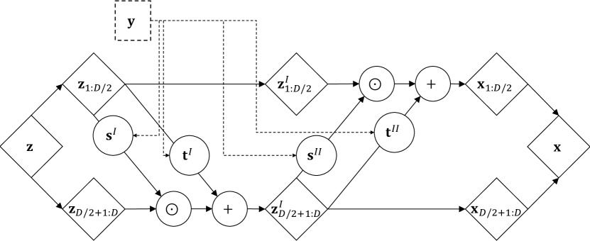
Figure 1: Example RealNVP architecture containing two conditional affine coupling layers (Dinh et al.,, 2017; Winkler et al.,, 2019), with conditioner models $\mathbf{s}^{I}$, $\mathbf{t}^{I}$, $\mathbf{s}^{II}$, and $\mathbf{t}^{II}$, Gaussian sample vector $\mathbf{z}$, data sample vector $\mathbf{x}$, intermediate sample vector $\mathbf{z}^{I}$, conditional input vector $\mathbf{y}$. The indices $1:D/2$ and $D/2+1:D$ refer to the two halves of the data vectors, respectively. The dashed lines indicate the flow of the conditional input data $\mathbf{y}$.

In this work, we employ the real non-volume preserving transformation (RealNVP) (Dinh et al.,, 2017), which is based on a composition of affine coupling layers. In each coupling layer, one half of the data vector undergoes an affine transformation, which is parameterized via functions of the remaining half of the data vector:

$$\mathbf{x}_{1:D/2}= \mathbf{z}_{1:D/2}$$ (3)

$$\mathbf{x}_{D/2+1:D}= \mathbf{z}_{D/2+1:D}\odot\exp(\mathbf{s}(\mathbf{z}_{1:D/2},\mathbf{y}))+\mathbf{t}(\mathbf{z}_{1:D/2},\mathbf{y})$$

Here, $\odot$ denotes element-wise multiplication, the indices $1:D/2$ and $D/2+1:D$ refer to the two halves of the data vectors, respectively, and $\mathbf{s}$ and $\mathbf{t}$ are the so-called conditioner models. Notably, the partial transformation of the data vectors keeps the inputs of $\mathbf{s}$ and $\mathbf{t}$ identical for both the forward and the inverse transformation. Thus, the conditioner models can be implemented as any standard feed forward neural network (Dinh et al.,, 2017). Furthermore, the clever design of the affine coupling layer results in lower triangular Jacobians. Hence, the Jacobian determinant required for the likelihood computation is simply given by the product over the diagonal elements. The log-form Jacobian determinant used for training then is:

$$\log\det\mathbf{J}_{\text{RealNVP}}(\mathbf{z})=\sum_{k=D/2+1}^{D}\mathbf{s}(\mathbf{z}_{1:D/2},\mathbf{y})$$

Large and highly expressive normalizing flows can be built using compositions of Equation (3) in an alternating manner. Figure 1 shows an illustrative sketch of an exemplary RealNVP architecture with two conditional affine coupling layers.

In Cramer et al., 2022b , we showed that normalizing flows sample uncharacteristically noisy scenarios when applied to sample for the distributions of renewable electricity time series, due to their inherent lower-dimensional manifold structure. To address the issue, we proposed dimensionality reduction based on the principal component analysis (PCA). In this work, we use PCA to reduce the dimensionality of the data $\mathbf{x}$ and the Gaussian samples $\mathbf{z}$. The conditional input vectors $\mathbf{y}$ are not affected by the PCA. For more information on the effects of manifolds we refer to Brehmer and Cranmer, (2020), Behrmann et al., (2021), and Cramer et al., 2022b .

3 Day-ahead scenario generation

This work addresses scenario generation with a particular focus on applications in day-ahead scheduling problems. Thus, all scenarios describe a possible realizations covering the time between 00:00 am and 11:59 pm of the following day. In particular, we generate day-ahead wind power generation scenarios and use day-ahead forecasts of wind speeds as conditional inputs to narrow down the range of possible trajectories and make the scenarios specific to the following day. For reference, we include a comparison to historical data, which represents unconditional scenarios, i.e., randomly drawn sampled from the full distribution $p_{X}(\mathbf{x})$ that does not consider the wind speed forecasts. Meanwhile, the scenario generation methods aim to fit models of the full conditional PDF $p_{X|Y}(\mathbf{x}|\mathbf{y})$ that are valid for every possible wind power realization $\mathbf{x}\in X$ and every possible day-ahead wind speed forecast $\mathbf{y}\in Y$. In the application, the wind speed predictions are known one day prior to the scheduling horizon and the scenario generation models are evaluated for fixed conditional inputs $\mathbf{y}$. Normalizing flows, Gaussian copulas, and W-GANs all employ multivariate modeling approaches, i.e., the models generate full daily trajectories in a vector form (Pinson et al.,, 2009; Ziel and Weron,, 2018; Chen et al., 2018b, ). All models use multivariate Gaussian samples $\mathbf{z}$ and the wind speed forecast vectors, i.e., the conditional information $\mathbf{y}$, as inputs to generate wind power generation scenario vectors $\mathbf{x}$. For a given fixed wind speed forecast $\mathbf{y}=\text{const.}$, sampling and transforming multiple Gaussian samples $\mathbf{z}$ results in a set of wind power generation scenarios, i.e., the Gaussian acts as a source of randomness to generate sets of scenarios instead of point forecasts:

$$\mathbf{x}_{i}=T(\mathbf{z}_{i},\mathbf{y}=\text{const.})\quad\forall i\in 1,\dots,\#\text{Scenarios}$$

Here, $T(\cdot)$ can be any of the scenario generation models. For more details on the evaluation of the different models, we refer to our supplementary material and the papers by Pinson et al., (2009) and Chen et al., 2018b .

All models generate capacity factor scenarios, i.e., the actual production scaled to installed capacity, of the 50 Hertz transmission grid in the years 2016 to 2020 (Open power systems data,, 2019). The year 2019 is set aside as a test set to avoid complications in the stochastic programming case study due to the unusual prices resulting from the COVID-19 pandemic (Michał Narajewski,, 2020; Badesa et al.,, 2021). To avoid including test data in the scenario sets, the unconditional historical scenarios are drawn from the training set. The 15 min recording interval renders 96-dimensional scenario vectors that fit the 24 h time horizon of a day-ahead bidding problem. The day-ahead wind speed forecasts have hourly resolution and are obtained from the reanalysis data set “Land Surface Forcings V5.12.4” of MERRA-2 (Global Modeling and Assimilation Office , 2015, GMAO) which is based on previously recorded historical data. We use the predictions at the coordinates 53.0^∘ N, 13.0^∘ E, in the center of the 50 Hertz region. Note that due to potential wind speed forecast errors and agglomeration effects in the power generation, there is no direct known functional relationship between the wind speed forecast and the realization of regionally distributed power generation.

Due to numerically singular Jacobians and non-invertible transformations (Behrmann et al.,, 2021; Cramer et al., 2022b, ), full-space normalizing flows fail to accurately describe the distribution of daily wind time series trajectories residing on lower-dimensional manifolds (Cramer et al., 2022b, ). Therefore, we use PCA (Pearson,, 1901) to reduce the data dimensionality following our recent contribution (Cramer et al., 2022b, ). We select the number of principal components based on the explained variance ratio, i.e., the amount of information maintained by the PCA (Pearson,, 1901). For an explained variance ratio of 99.95%, we obtain 18 principal components to represent the original 96-dimensional scenario vectors. The adversarial training algorithm for the W-GAN (Arjovsky et al.,, 2017) did not converge consistently for the considered learning problem. Thus, the results presented below are drawn from the best performing model out of 20 different trained models w.r.t. the metrics outlined in Section 4. For more detailed information on the implementation, we refer to the supplementary material.

4 Conditional wind power scenario generation

We start by analyzing the scenarios without a specific application in mind. To this end, we present some examples, analyze the described distributions, and investigate whether the models can identify the correct daily trends.

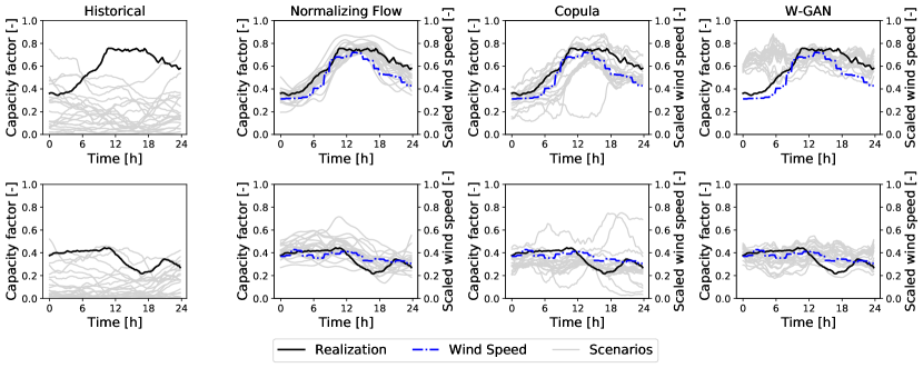
Figure 2: 20 wind capacity factor scenarios (“Scenarios”) each from the historical scenario set (left), normalizing flow (center-left), Gaussian copula (center-right), and W-GAN (right) in relation to the realized wind capacity factor (“Realization”). The plots for the the scenario generation methods include the conditional input (“Wind Speed”). Realization and scenarios on the left y-axis and scaled wind speed predictions on right y-axis. Top: March 29th, 2019, bottom: September 15th, 2019. Data from 50 Hertz region (Open power systems data,, 2019).

Figure 2 shows example scenarios for two randomly selected days of the test year 2019. The left, center-left, center-right, and right columns show historical scenarios and scenarios sampled from the conditional normalizing flow, the Gaussian copula, and the W-GAN, respectively. The historical scenarios are randomly selected from the training set and are, therefore, unspecific to the respective days. Thus, they fail to identify the daily trends and show large discrepancies for both days. For both example days in Figure 2 the normalizing flow identifies and follows the general trend of the realized wind capacity factor. For the presented examples, the realization lies within the span of the scenarios. Similarly, the Gaussian copula also identifies the trend of the realization. However, there are some scenarios with significantly higher or lower capacity factors in the case of both days, i.e., the Gaussian copula appears prone to sample outliers that do not follow the trend. The W-GAN-generated scenarios fail to identify the trend and, instead, appear tightly agglomerated and only represent the daily average of the realization, which can be observed for the morning hours of the first day and, to a lesser extend, on the afternoon hours of the second day. The failed identification of the trend is likely due to a mode collapse of the W-GAN, which is a frequently observed phenomenon with GANs (Arjovsky and Bottou,, 2017). Mode collapse happens when the adversarial training algorithm converges to a small range of realistic scenarios but fails to identify the true distribution. Note that due to the multivariate modeling approach of generating full daily trajectories, this type of deviation may occur at any time step throughout the day.

To gain insight into the quality of the full scenario sets, we analyze whether the scenario generation methods are able to reproduce the probability distributions and the frequency behavior of the actual time series by looking at the full year of 2019 in comparison to the eventual realization. To this end, we look into the marginal PDF (Parzen,, 1962), the quantile distribution in Q-Q plots (Chambers,, 2018), and the power spectral density (PSD) (Welch,, 1967). For a detailed introduction to the interpretation of PDF and PSD, we refer to our previous work (Cramer et al., 2022a, ). Figure 3 shows the marginal PDFs (left), the Q-Q plots (center), and the PSD (right) of the historical- and the generated scenarios from the normalizing flow, the Gaussian copula, and the W-GAN in comparison to the realizations in 2019.

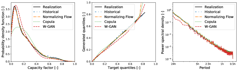
Figure 3: Distribution and fluctuational behavior of generated wind capacity factor scenarios from historical training data (“Historical”), normalizing flow (“Normalizing Flow”), Gaussian copula (“Copula”), and W-GAN (“W-GAN”) in comparison to historical test data (“Realization”) (Open power systems data,, 2019). Left: marginal probability density function (PDF) estimated using kernel density estimation (Parzen,, 1962), center: quantile-quantile plots (Q-Q-plots) (Chambers,, 2018), right: power spectral density (PSD) estimated using Welch’s method (Welch,, 1967).

In Figure 3, the historical scenarios and the normalizing flow scenarios describe the test set PDF well and show good matches of the quantile distribution in the Q-Q-plot. Meanwhile, the Gaussian copula produces a broader PDF with a much lower peak than the realization, whereas the W-GAN’s PDF shows a shift towards higher values. The Q-Q-plot also shows the shift of the W-GAN generated distribution, as there is an offset between the W-GANs and the other quantile lines. The poor distribution match by the Gaussian copula is likely due to the linear quantile regression that is unable to represent the nonlinear relation between the predicted wind speed and the capacity factor. Furthermore, the copula relies on linear interpolation of quantiles which can inflate the PDF in the tails and, thus, lead to outlier sampling (Pinson et al.,, 2009). The W-GAN can theoretically model any distribution (Goodfellow et al.,, 2014). In our analysis, however, the adversarial training algorithm was very difficult to handle with the time series data and often resulted in poor fits. The presented results are the best of 20 training runs in terms of matching the criteria in Figure 3. Meanwhile, both the Gaussian copula and the normalizing flow with PCA converge consistently and typically yield the presented results after the first training attempt.

The Q-Q-plot reveals that all methods yield distributions with longer tails than the realizations, i.e., they produce scenarios with higher capacity factors than the maximum realized capacity factor. The reason is that for days with the highest capacity factor of the year, even higher capacity factors are still feasible as the realizations never reach the full installed capacity. Also, the log tail of the PDF makes the offset appear inflated as it only occurs for the 99-th and 100-th percentile. Note that both Copula and W-GAN are restricted to sample from the [0,1] interval via the boundaries of the inverse CDF (Pinson et al.,, 2009) and the tanh output activation function, respectively. Meanwhile, the normalizing flow has no such restriction and yields some scenarios surpassing 1, which leads to the normalizing flow having the strongest deviation in the Q-Q-plot. Although these scenarios are theoretically infeasible, they have a very low probability and can efficiently be removed in postprocessing.

The PSD in Figure 3 shows a good match of the frequency behavior by the historical scenarios, the normalizing flow, and the Gaussian copula. The W-GAN is close to the overall power-law, i.e., the slope of the PDF curve, of the data, but fails to match the exact frequency behavior.

In addition to the analysis of the full scenario sets in Figure 3, we also compute the energy score (ES) for each day in 2019. ES is a quantitative measure for the assessment of multivariate scenario generation models that compares the conditional scenario set with the respective realization (Gneiting et al.,, 2008; Pinson and Girard,, 2012):

$$\text{ES}=\frac{1}{N_{S}}\sum_{s=1}^{N_{S}}||\mathbf{x}-\hat{\mathbf{x}}_{s}||_{2}-\frac{1}{2{N_{S}}^{2}}\sum_{s=1}^{N_{S}}\sum_{s^{\prime}=1}^{N_{S}}||\hat{\mathbf{x}}_{s}-\hat{\mathbf{x}}_{s^{\prime}}||_{2}$$

Here, $\mathbf{x}$ is the realization vector, $\hat{\mathbf{x}}_{s}$ are the scenario vectors, $N_{S}$ is the number of scenarios, and $||\cdot||_{2}$ is the 2-norm. The energy score is a negatively oriented score, i.e., lower values indicate better results. The two parts of the energy score reward closeness to the realization and diversity of the scenario set, respectively.

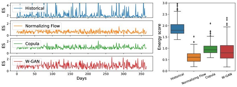
Figure 4: Energy score (ES) (Gneiting et al.,, 2008; Pinson and Girard,, 2012) over all days in 2019 (left) and boxplots (right). Historical- (“Historical”) and generated scenarios from normalizing flow (“Normalizing Flow”), Gaussian copula (“Copula”), and Wasserstein-GAN (“W-GAN”). Boxes indicate quartiles and diamonds indicate outliers (Waskom,, 2021). Note different y-scale for historical ES.

In Figure 4, we display the energy score for each day in 2019 as well as boxplots that showcase the overall energy score distributions for the historical data and the three different models. The normalizing flow energy score is lower on average compared to the Gaussian copula and the W-GAN, indicating a better fitting of the realizations and more diverse scenarios. The Gaussian copula shows the highest energy score which is likely a result of the outliers observed in Figure 2. Furthermore, the normalizing flow leads to a narrow distribution of energy scores with few outliers, indicating consistently good results. Meanwhile, the historical scenarios consistently result in significantly higher energy scores compared to the conditional day-ahead scenario generation methods. By design, the unconditional historical scenarios do not identify the daily trends and are not generated specifically for the respective days. Thus, the deviations from the realizations penalized by the energy score are significant for most days.

In conclusion, we find that the conditional normalizing flow presented in Section 2 generates scenarios that match the true distribution of realizations closely, while also providing a diverse set of possible realizations. Furthermore, the normalizing flow outperforms the Gaussian copula and the W-GAN with respect to all important metrics. The historical scenarios describe the overall distribution well, but are not specific to the individual days and, hence, return poor results in day-ahead problem-specific metrics like the energy score.

5 Day-ahead bidding strategy optimization

We apply the scenarios generated in the previous section in a wind producer bidding problem based on Garcia-Gonzalez et al., (2008) and Conejo et al., (2010). We first state the problem formulation and then analyze the stability of the scenario generation methods for different numbers of scenarios based on the criterion defined by Kaut and Wallace, (2003). Finally, we investigate the obtained profits based on the different scenario sets.

5.1 Wind producer problem formulation

We consider the deterministic equivalent formulation (Birge and Louveaux,, 2011) of the stochastic wind producer problem from Garcia-Gonzalez et al., (2008) and Conejo et al., (2010) shown in Figure 5 that aims to find an optimal bidding schedule for the operator of a wind farm participating in the European Power Exchange (EPEX SPOT) market (European Power Exchange,, 2021).

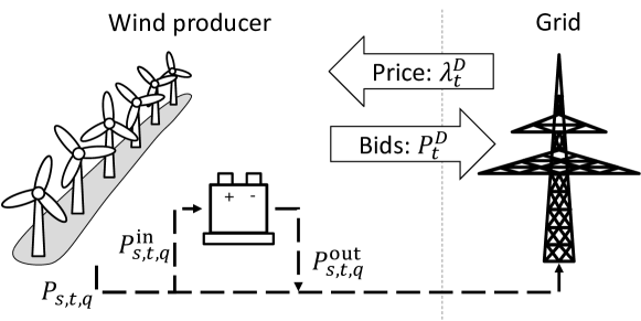
Figure 5: Structural setup of the wind producer problem from Garcia-Gonzalez et al., (2008) and Conejo et al., (2010) with generated electricity $P_{s,t,q}$, (dis-) charging rates $P_{s,t,q}^{\text{in}}$ and $P_{s,t,q}^{\text{out}}$, placed bids $P_{t}^{D}$, and day-ahead electricity prices $\lambda_{t}^{D}$. The indices $s$, $t$, and $q$ indicate scenarios, hourly time intervals, and quaterhourly time intervals, respectively.

First, the operator places bids at the day-ahead auction market one day prior to delivery and, thereby, commits to deliver a certain amount of electricity $P^{D}_{t}$ during the given trading time interval $t$. The revenue made is given by $\lambda^{D}_{t}P^{D}_{t}\delta_{h}$, where $\lambda^{D}_{t}$ is the day-ahead price and $\delta_{h}=1\,h$ is the trading interval. As wind electricity generation is stochastic and non-dispatchable (Conejo et al.,, 2010), the placed bids may not always be met by the actual production. To balance the difference between the placed bids and the actual production we allow for a small electricity storage that can store the electricity of up to 15 min of maximum production. For any remaining production imbalance, we enforce a penalty on the absolute value of the imbalance (Garcia-Gonzalez et al.,, 2008). The full objective then reads (Garcia-Gonzalez et al.,, 2008):

$$\underset{P^{D}_{t}}{\operatorname{max}}\sum_{t=1}^{N_{T}}\left[\lambda^{D}_{t}P^{D}_{t}\delta_{h}-\omega|\lambda^{D}_{t}|\sum_{s=1}^{N_{S}}\pi_{s}|\Delta_{s,t}|\right]$$ (4)

Here, $\Delta_{t,s}$ is the imbalance at time point $t$ and scenario $s$. The penalty term is based on the absolute values of the day-ahead price $|\lambda^{D}_{t}|$ to compensate for possible negative electricity prices (Garcia-Gonzalez et al.,, 2008).

The penalty term in Equation (4) contains the absolute value operator $|\cdot|$, leading to a nonlinear problem. However, any positive deviation can be avoided via curtailment of the plant and the imbalance will only take negative values in practice, which makes the absolute value operator obsolete. Thus, the absolute imbalance is substituted by its negative parts to obtain a linear problem (Conejo et al.,, 2010). The complete linear formulation of the wind producer market participation problem including the electricity storage is shown in Problem (WP).

$$\underset{P^{D}_{t},P^{\text{in}}_{s,t,q},P^{\text{out}}_{s,t,q}}{\operatorname{max}} \sum_{t=1}^{N_{T}}\left[\lambda^{D}_{t}P^{D}_{t}\delta_{h}-\omega|\lambda^{D}_{t}|\sum_{s=1}^{N_{S}}\pi_{s}\Delta^{-}_{s,t}\right]$$ (WP)

s.t. $$\text{SOC}_{s,t,q}=\text{SOC}_{s,t,q-1}+\eta\delta_{q}P^{\text{in}}_{s,t,q}-\frac{1}{\eta}\delta_{q}P^{\text{out}}_{s,t,q}, \forall s\in\mathcal{S},\forall t\in\mathcal{T},\forall q\in\mathcal{Q}$$

$$\text{SOC}_{s,t=24,q=4}=\text{SOC}_{0}, \forall s\in\mathcal{S}$$

$$\Delta^{-}_{s,t}\leq\delta_{h}P^{D}_{t}-\delta_{q}\sum_{q\in\mathcal{Q}}P_{s,t,q}-\left(P^{\text{out}}_{s,t,q}-P^{\text{in}}_{s,t,q}\right), \forall s\in\mathcal{S},\forall t\in\mathcal{T}$$

$$0\leq P^{D}_{t}\leq P^{D,\operatorname{max}}, \forall t\in\mathcal{T}$$

$$0\leq\Delta^{-}_{s,t}, \forall s\in\mathcal{S},\forall t\in\mathcal{T}$$

$$0\leq P^{\text{in}}_{s,t,q}\leq P^{\operatorname{max}}, \forall s\in\mathcal{S},\forall t\in\mathcal{T},\forall q\in\mathcal{Q}$$

$$0\leq P^{\text{out}}_{s,t,q}\leq P^{\operatorname{max}}, \forall s\in\mathcal{S},\forall t\in\mathcal{T},\forall q\in\mathcal{Q}$$

$$0\leq\text{SOC}_{s,t,q}\leq\text{SOC}^{\operatorname{max}}, \forall s\in\mathcal{S},\forall t\in\mathcal{T},\forall q\in\mathcal{Q}$$

$$\mathcal{S}=\{1,\dots,N_{S}\}$$

$$\mathcal{T}=\{1,\dots,N_{T}\}$$

$$\mathcal{Q}=\{1,\dots,4\}$$

Tables 1, 2, and 3 list the indices, parameters, and variables of Problem (WP), respectively. Problem (WP) is the deterministic equivalent of a two-stage stochastic program (Birge and Louveaux,, 2011), where the delivery commitments are the first stage decisions and, the second stage decisions are the actual delivery and the storage operation.

The problem is implemented in pyomo (Hart et al.,, 2017), version 6.2, and solved using gurobi (Gurobi Optimization, LLC,, 2021), version 9.5.

Table 1: Indices in Problem (WP).

Indices	Description
$q$	Quater hour interval
$s$	Scenarios
$t$	Hour interval

Table 2: Parameters in Problem (WP).

Parameter	Description	Value/Unit
$\delta_{h}$	Trading time interval	1 h
$\delta_{q}$	Production time interval	15 min
$\eta$	(Dis-) Charging efficiency	0.91
$\lambda^{D}_{t}$	Day-Ahead Price	[EUR/MWh]
$\omega$	Penalty factor	1.5
$\pi_{s}$	Probability of scenario s	$1/N_{S}$
$N_{T}$	Number of time steps	24
$N_{S}$	Number of scenarios	[-]
$P^{D,\operatorname{max}}$	Maximum production capacity	100 MW
$P^{\operatorname{max}}$	Maximum (dis-) charging rate	12.5 MW
$P_{s,t,q}$	Actual production	[MW]
$\text{SOC}^{\operatorname{max}}$	Maximum battery capacity	25 MWh
$\text{SOC}_{0}$	Initial battery state of charge	12.5 MWh

Table 3: Variables in Problem (WP).

Variable	Description	Unit
$P^{D}_{t}$	Bid at day-ahead market	[MW]
$P^{in}_{s,t,q}$	Charging rate	[MW]
$P^{out}_{s,t,q}$	Discharging rate	[MW]
$\text{SOC}_{s,t,q}$	Battery state of charge	[MWh]
$\Delta^{-}_{s,t}$	Negative production imbalance	[MW]

Note that in Problem (WP), simultaneous charging and discharging of the storage is feasible, however, does not occur at the optimum due to the losses associated with using the storage. The problem operates on both the trading time scale with hourly intervals and the production time scales with 15 min intervals.

5.2 Stability

Kaut and Wallace, (2003) define stability and bias as criteria for the quality of a scenario generation method for stochastic programming. A scenario generation method is considered stable when different instances of the stochastic program based on different generated scenario sets result in similar optimal objective values. A small bias is achieved if the optimal objective value of the scenario-based formulation is close to the optimal objective value obtained by solving the stochastic program with the true distribution of the uncertain parameter. For the case of day-ahead scenario generation methods, the biases of the scenario generation methods are impossible to assess, as the true distribution for the wind power generation of the individual days is unknown and cannot be represented via historical data.

Problem WP is linear and can be solved efficiently. However, larger mixed-integer problems, as well as non-convex stochastic programs, often cannot be solved for a large number of scenarios due to the large computational effort (Birge and Louveaux,, 2011) and, small scenario sets must suffice for the stochastic program. Consequently, high stability becomes increasingly important for small numbers of scenarios. In the following, we solve 50 instances of Problem (WP) for each day of 2019 and each scenario generation method using small scenario sets of only 3, 5, 10, 20, and 50 scenarios, each.

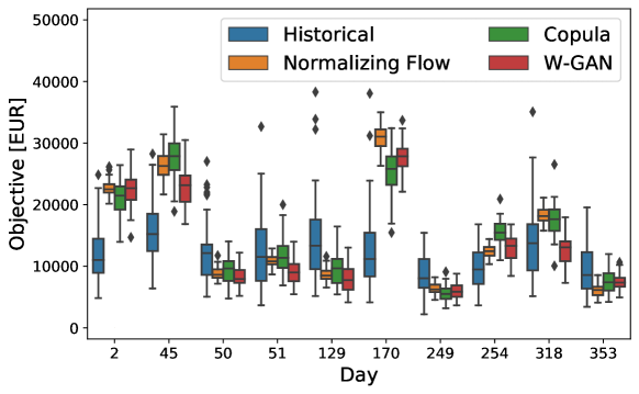
Figure 6: Boxplot of the optimal objective function distributions for 50 instances of Problem (WP) with five scenarios from the historical data set (“Historical”), normalizing flow (“Normalizing Flow”), Gaussian copula (“Copula”), and W-GAN (“W-GAN”), respectively. Boxes indicate quartiles and diamonds indicate outliers (Waskom,, 2021).

Figure 6 shows box plots of the optimal objectives using small sets of five scenarios from the historical data set, normalizing flow, Gaussian copula, and W-GAN for ten randomly selected days from 2019. As an indicator of stability, we look at the spread of optimal objectives, i.e., the height of the box plots, that result from the 50 different scenario sets. For the ten randomly selected days shown in Figure 6, the normalizing flow scenarios result in the lowest spreads of optimal objectives. The optimal objectives of the Gaussian copula scenarios show significantly larger spreads than both the normalizing flow and the W-GAN scenarios. Meanwhile, the randomly selected historical scenario sets lead to by far the largest spreads.

Table 4: Average standard deviation (StD) and average max-min spread (Spread) of the optimal objectives of 50 different instances of Problem (WP) with 3, 5, 10, 20, and 50 scenarios each generated from normalizing flow, Gaussian copula, and W-GAN over all days in 2019. Best results are marked in bold font.

	# Scenarios	Historical	Normalizing Flow	Copula	W-GAN
StD [EUR]	3	6735	1726	3534	2441
	5	5025	1317	2585	1883
	10	3291	930	1763	1333
	20	2253	659	1244	932
	50	1404	417	787	593
Spread [EUR]	3	30527	7874	17467	10719
	5	22899	5979	12285	8367
	10	14963	4214	8142	5966
	20	10138	3017	5613	4184
	50	6371	1891	3531	2675

Table 4 shows statistics for the different numbers of scenarios derived over all days in 2019, namely, the average standard deviation and the max-min spread, i.e., the difference between the maximum and minimum objective value. The results in Table 4 confirm the observation from Figure 6 that normalizing flows yield scenarios with the most stable optimal objectives indicated by the lowest standard deviation and the lowest spread. Furthermore, both standard deviations and spreads decrease for increasing numbers of scenarios for all scenario generation methods. Notably, the normalizing flow achieves greater stability with fewer scenarios compared to the other methods. For instance, the standard deviation achieved with just three normalizing flow scenarios is lower than the standard deviations of ten Gaussian copula scenarios and lower than five W-GAN scenarios.

It appears that the outlier scenarios of the Gaussian copula observed in Figure 2 are weighted more heavily in the case of only a few scenarios and, thus, lead to larger differences in the optimal objectives. As the normalizing flow shows no extreme outlier scenarios and identifies the overall trends well, there is very little variance in the optimal objective values even for small scenario sets. The historical data results in the largest spreads as the data is sampled from the entire spectrum of possible realizations instead of the narrower distributions described by the day-ahead scenario generation models.

5.3 Obtained profits

Solving Problem (WP) maximizes the expected profits and yields first-stage decisions that describe a fixed schedule of electricity delivery commitments for the day-ahead market $P^{D}_{t}$. We can compute the actual profits by fixing the first stage decisions obtained from the stochastic program and re-optimizing the second stage with the realized electricity production. To gain statistically relevant results, we compute the actual profits obtained in Problem (WP) for each day in 2019, each time using 100 historical or generated scenarios. For comparison, we also compute the profits obtained via the perfect foresight problem, i.e., an ideal single scenario instance of Problem (WP) based on the actual realization.

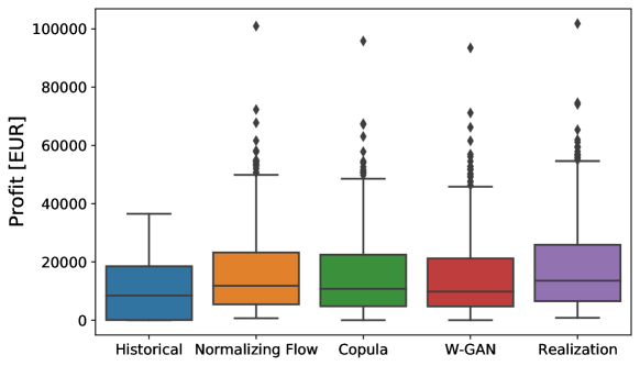
Figure 7: Boxplot of profits obtained in 2019 in Problem (WP). Each problem uses 100 scenarios generated from the historical data (“Historical”), the normalizing flow (“Normalizing Flow”), the Gaussian copula (“Copula”), and the W-GAN (“W-GAN”) or the realization for the perfect foresight (“Realization”), respectively. Boxes indicate quartiles and diamonds indicate outliers (Waskom,, 2021).

Figure 7 shows box plots of the distribution of profits obtained by using scenarios from the historical data and the three different generation methods in comparison to the profits obtained from the perfect foresight problem (“Realization”). The profits obtained by using the normalizing flow scenarios are the highest, while the Gaussian copula scenarios yield profits between the normalizing flow and the W-GAN. The profits obtained by using the unconditional historical scenarios are significantly lower than those of all models generating day-ahead scenarios. Furthermore, the historical scenarios are unconditional and fail to identify the days with high production that appear as high-profit outliers in the case of the other scenario generation methods and the perfect foresight case.

Table 5: Average, average percentage, and maximum perfect information profit gap (PIPG) of actual profits obtained over all days in 2019 with 100 scenarios each generated from normalizing flow, Gaussian copula, and W-GAN, respectively. Best results are marked in bold font.

	Historical	Normalizing Flow	Copula	W-GAN
Average PIPG [EUR]	-8381	-1832	-2658	-3485
Average PIPG [%]	-81.5%	-10.9%	-16.6%	-23.0%
Max. PIPG [EUR]	-70234	-8311	-11017	-17432

To analyze whether the scenario generation methods take advantage of the profit potentials, we define the perfect information profit gap (PIPG) as the difference between the actual profits obtained from the stochastic program and the perfect information profit. Table 5 lists the average and maximum PIPGs in 2019. The average PIPGs show that the normalizing flow scenarios yield profits that are on average 6% and 12% points closer to the perfect foresight profits compared to the Gaussian copula and the W-GAN, respectively. Meanwhile, the historical scenario profits are over 80% lower on average than the perfect foresight profit. The maximum PIPG, i.e., the worst performing days, also show that the normalizing flow scenarios give significantly more profitable results compared to the other generation methods.

Table 6: Average expected profits (“Average objective [EUR]”) of the stochastic program and average actual profits (“Average profit [EUR]”) of 50 different instances of Problem (WP) with 3, 5, 10, 20, and 50 scenarios each from the historical data and generated from the normalizing flow, the Gaussian copula, and the W-GAN over all days in 2019.

	# Scenarios	Historical	Normalizing Flow	Copula	W-GAN
Average objective [EUR]	3	12268	17336	16435	16011
Average profit [EUR]		5753	16156	13527	14694
Average objective [EUR]	5	11890	17195	16196	15880
Average profit [EUR]		7544	16438	15197	14813
Average objective [EUR]	10	10821	16974	15833	15646
Average profit [EUR]		8390	16628	15738	14988
Average objective [EUR]	20	10305	16893	15675	15530
Average profit [EUR]		8864	16725	15880	15103
Average objective [EUR]	50	10004	16829	15597	15464
Average profit [EUR]		9132	16792	15984	15170

Table 6 lists the average expected profits (“Average objective [EUR]”) and the average actual profits (“Average profit [EUR]”) obtained using scenario sets of size 3, 5, 10, 20, and 50. For all scenario generation methods, smaller scenario sets tend to overestimate the expected profits. For increasing numbers of scenarios, the expected profits and the actual profits converge. Notably, the normalizing flow scenarios result in the smallest difference between the expected and the actual profits, particularly for smaller scenario sets of three or five scenarios. Furthermore, the average actual profits obtained using the normalizing flow are consistently higher than the actual profits obtained from any of the other methods. In fact, using just three normalizing flow scenarios results in higher profits than any investigated number of scenarios from any other considered scenario generation method.

The higher profits obtained using the normalizing flow scenarios reflect the findings of Section 4, i.e., the normalizing flow identifies the correct trends and also reflects a diverse distribution. Meanwhile, the Gaussian copula shows outliers and does not match the distribution, and the W-GAN even struggles to identify the daily trends. The unconditional historical scenarios do not describe the daily trends and, thus, result in significantly lower profits in the day-ahead scheduling optimization. In conclusion, the results shown in Figure 7, Table 5, and Table 6 highlight that the normalizing flow generates the best scenarios and yields the most profitable bids.

6 Conclusion

The present work considers the scenario generation problem for a day-ahead bidding problem of a wind farm operator to participate in the EPEX spot markets. We utilize a data-driven multivariate scenario generation scheme based on conditional normalizing flows to model the distribution of wind capacity factor trajectories with wind speed predictions as conditional inputs. The generated scenarios are specifically tailored to stochastic optimization problems concerning the time frame between 00:00 am and 11:59 pm.

We analyze the normalizing flow scenarios in comparison to randomly selected historical data and scenarios generated from other more established methods, namely, Gaussian copulas and Wasserstein generative adversarial networks (W-GANs), and compare them to the actually realized power generation in 2019. The historical scenarios reflect the overall distribution of realizations well but fail to identify daily trends and show large variations independent of the investigated day. Among the conditional scenario generation methods, the normalizing flow scenarios best reflect the realized power generation trends and their distributions while also displaying a diverse set of possible realizations. Meanwhile, the Gaussian copula results in uncharacteristic outliers, and the W-GAN struggles to identify the main trends of the realizations. Furthermore, both Gaussian copula and W-GAN result in skewed distributions.

To assess their value for stochastic programming, the scenarios are applied in a stochastic programming case study that aims to set bids for electricity sales on the day-ahead market. First, we investigate the stability defined by Kaut and Wallace, (2003). Here, the normalizing flow yields scenarios that result in the most stable optimal objective values, even for small scenario sets. In particular, the normalizing flow scenarios result in the smallest standard deviation and the smallest spread in the optimal objective values. The analysis of the actual profits obtained on all days of 2019 shows a significant advantage of using day-ahead scenarios that are specifically tailored to the investigated day. Using randomly selected historical scenarios results in an average perfect information profit gap (PIPG) of over 80%, while the conditional scenario generation methods return PIPGs between 10 to 23%. The bids placed using the normalizing flow scenarios obtain the highest profits and have the lowest PIPG, i.e., the profits are closest to the perfect foresight profits. Notably, even small scenario sets of only three normalizing flow scenarios result in higher actual profits than any investigated number of scenarios from the other considered scenario generation methods.

In conclusion, utilizing conditional, day-specific scenarios in day-ahead scheduling problems leads to significantly more profitable decisions compared to relying on unconditional historical data. Furthermore, the conditional normalizing flow model yields high-quality scenarios that result in highly profitable solutions for stochastic programs and stable results, even for small scenario sets. Therefore, we argue that normalizing flow scenarios have a high potential for scheduling problems that cannot be solved with a large scenario set.

Bibliography

- Arjovsky and Bottou, (2017) Arjovsky, M. and Bottou, L. (2017). Towards principled methods for training generative adversarial networks. arXiv preprint arXiv:1701.04862.
- Arjovsky et al., (2017) Arjovsky, M., Chintala, S., and Bottou, L. (2017). Wasserstein generative adversarial networks. In International Conference on Machine Learning, pages 214–223, Sydney, Australia. PMLR.
- Badesa et al., (2021) Badesa, L., Strbac, G., Magill, M., and Stojkovska, B. (2021). Ancillary services in Great Britain during the COVID-19 lockdown: A glimpse of the carbon-free future. Applied Energy, 285:116500.
- Behrmann et al., (2021) Behrmann, J., Vicol, P., Wang, K.-C., Grosse, R., and Jacobsen, J.-H. (2021). Understanding and mitigating exploding inverses in invertible neural networks. In Banerjee, A. and Fukumizu, K., editors, Proceedings of The 24th International Conference on Artificial Intelligence and Statistics, volume 130 of Proceedings of Machine Learning Research, pages 1792–1800. PMLR.
- Birge and Louveaux, (2011) Birge, J. R. and Louveaux, F. (2011). Introduction to stochastic programming. Springer Science & Business Media, New York, US.
- Borji, (2019) Borji, A. (2019). Pros and cons of GAN evaluation measures. Computer Vision and Image Understanding, 179:41–65.
- Brehmer and Cranmer, (2020) Brehmer, J. and Cranmer, K. (2020). Flows for simultaneous manifold learning and density estimation. Advances in Neural Information Processing Systems, 33:442–453.
- Camal et al., (2019) Camal, S., Teng, F., Michiorri, A., Kariniotakis, G., and Badesa, L. (2019). Scenario generation of aggregated wind, photovoltaics and small hydro production for power systems applications. Applied Energy, 242:1396–1406.
- Chambers, (2018) Chambers, J. M. (2018). Graphical methods for data analysis, volume 1. CRC Press, 1 edition.
- (10) Chen, S., Guo, Z., Liu, P., and Li, Z. (2018a). Advances in clean and low-carbon power generation planning. Computers & Chemical Engineering, 116:296–305. Multi-scale Systems Engineering – in memory & honor of Professor C.A. Floudas.
- (11) Chen, Y., Wang, Y., Kirschen, D., and Zhang, B. (2018b). Model-free renewable scenario generation using generative adversarial networks. IEEE Transactions on Power Systems, 33(3):3265–3275.
- Conejo et al., (2010) Conejo, A. J., Carrión, M., and Morales, J. M. (2010). Decision Making Under Uncertainty in Electricity Markets, volume 1. Springer Science & Buisness Media, Boston, MA, 1 edition.
- (13) Cramer, E., Gorjão, L. R., Mitsos, A., Schäfer, B., Witthaut, D., and Dahmen, M. (2022a). Validation methods for energy time series scenarios from deep generative models. IEEE Access, 10:8194–8207.
- (14) Cramer, E., Mitsos, A., Tempone, R., and Dahmen, M. (2022b). Principal component density estimation for scenario generation using normalizing flows. Data-Centric Engineering, 3:e7.
- Dinh et al., (2017) Dinh, L., Sohl-Dickstein, J., and Bengio, S. (2017). Density estimation using Real NVP. In 5th International Conference on Learning Representations, ICLR 2017, Toulon, France, April 24-26, 2017, Conference Track Proceedings. OpenReview.net.
- (16) Dumas, J., Cointe, C., Wehenkel, A., Sutera, A., Fettweis, X., and Cornélusse, B. (2022a). A probabilistic forecast-driven strategy for a risk-aware participation in the capacity firming market. IEEE Transactions on Sustainable Energy, 13(2):1234–1243.
- (17) Dumas, J., Wehenkel, A., Lanaspeze, D., Cornélusse, B., and Sutera, A. (2022b). A deep generative model for probabilistic energy forecasting in power systems: Normalizing flows. Applied Energy, 305:117871.
- European Power Exchange, (2021) European Power Exchange (2021). EPEX SPOT documentation. \urlhttp://www.epexspot.com/en/extras/ download-center/documentation. Accessed: 2021-05-30.
- Garcia-Gonzalez et al., (2008) Garcia-Gonzalez, J., de la Muela, R. M. R., Santos, L. M., and Gonzalez, A. M. (2008). Stochastic joint optimization of wind generation and pumped-storage units in an electricity market. IEEE Transactions on Power Systems, 23(2):460–468.
- Ge et al., (2020) Ge, L., Liao, W., Wang, S., Bak-Jensen, B., and Pillai, J. R. (2020). Modeling daily load profiles of distribution network for scenario generation using flow-based generative network. IEEE Access, 8:77587–77597.
- Global Modeling and Assimilation Office , 2015 (GMAO) Global Modeling and Assimilation Office (GMAO) (2015). MERRA-2 inst1_2d_lfo_Nx: 2d, 1-Hourly, Instantaneous, Single-Level, Assimilation, Land Surface Forcings V5.12.4, Greenbelt, MD, USA, Goddard Earth Sciences Data and Information Services Center (GES DISC). Accessed: 2022-01-21, 10.5067/RCMZA6TL70BG.
- Gneiting et al., (2008) Gneiting, T., Stanberry, L. I., Grimit, E. P., Held, L., and Johnson, N. A. (2008). Assessing probabilistic forecasts of multivariate quantities, with an application to ensemble predictions of surface winds. Test, 17(2):211–235.
- Goodfellow et al., (2014) Goodfellow, I., Pouget-Abadie, J., Mirza, M., Xu, B., Warde-Farley, D., Ozair, S., Courville, A., and Bengio, Y. (2014). Generative adversarial nets. In Advances in Neural Information Processing Systems, pages 2672–2680. MIT Press, Cambridge, MA, USA.
- Grossmann, (2021) Grossmann, I. E. (2021). Advanced Optimization for Process Systems Engineering. Cambridge Series in Chemical Engineering. Cambridge University Press.
- Grossmann and Sargent, (1978) Grossmann, I. E. and Sargent, R. (1978). Optimum design of chemical plants with uncertain parameters. AICHE journal, 24(6):1021–1028.
- Gurobi Optimization, LLC, (2021) Gurobi Optimization, LLC (2021). Gurobi Optimizer Reference Manual.
- Halemane and Grossmann, (1983) Halemane, K. P. and Grossmann, I. E. (1983). Optimal process design under uncertainty. AIChE Journal, 29(3):425–433.
- Hart et al., (2017) Hart, W. E., Laird, C. D., Watson, J.-P., Woodruff, D. L., Hackebeil, G. A., Nicholson, B. L., Siirola, J. D., et al. (2017). Pyomo-optimization modeling in python, volume 67. Springer.
- Jiang et al., (2018) Jiang, C., Mao, Y., Chai, Y., Yu, M., and Tao, S. (2018). Scenario generation for wind power using improved generative adversarial networks. IEEE Access, 6:62193–62203.
- Kaut and Wallace, (2003) Kaut, M. and Wallace, S. W. (2003). Evaluation of scenario-generation methods for stochastic programming. Humboldt-Universität zu Berlin, Mathematisch-Naturwissenschaftliche Fakultät II, Institut für Mathematik, Berlin, Germany.
- Kobyzev et al., (2020) Kobyzev, I., Prince, S. J., and Brubaker, M. A. (2020). Normalizing flows: An introduction and review of current methods. IEEE Transactions on Pattern Analysis and Machine Intelligence, 43(11):3964–3979.
- Leo et al., (2021) Leo, E., Dalle Ave, G., Harjunkoski, I., and Engell, S. (2021). Stochastic short-term integrated electricity procurement and production scheduling for a large consumer. Computers & Chemical Engineering, 145:107191.
- Liu et al., (2015) Liu, G., Xu, Y., and Tomsovic, K. (2015). Bidding strategy for microgrid in day-ahead market based on hybrid stochastic/robust optimization. IEEE Transactions on Smart Grid, 7(1):227–237.
- Mayer and Trück, (2018) Mayer, K. and Trück, S. (2018). Electricity markets around the world. Journal of Commodity Markets, 9:77–100.
- Michał Narajewski, (2020) Michał Narajewski, F. Z. (2020). Changes in electricity demand pattern in europe due to COVID-19 shutdowns. IAEE Energy Forum, pages 44–47.
- Mitsos et al., (2018) Mitsos, A., Asprion, N., Floudas, C. A., Bortz, M., Baldea, M., Bonvin, D., Caspari, A., and Schäfer, P. (2018). Challenges in process optimization for new feedstocks and energy sources. Computers & Chemical Engineering, 113:209–221.
- Morales et al., (2013) Morales, J. M., Conejo, A. J., Madsen, H., Pinson, P., and Zugno, M. (2013). Integrating Renewables in Electricity Markets: Operational Problems, volume 205. Springer Science & Business Media, Boston, MA, 1 edition.
- Open power systems data, (2019) Open power systems data (2019). Time series. \urlhttps://open-power-system-data.org/. Accessed: 2020-03-30.
- Papamakarios et al., (2021) Papamakarios, G., Nalisnick, E., Rezende, D. J., Mohamed, S., and Lakshminarayanan, B. (2021). Normalizing flows for probabilistic modeling and inference. Journal of Machine Learning Research, 22(57):1–64.
- Parzen, (1962) Parzen, E. (1962). On estimation of a probability density function and mode. The Annals of Mathematical Statistics, 33(3):1065–1076.
- Pearson, (1901) Pearson, K. (1901). On lines and planes of closest fit to systems of points in space. The London, Edinburgh, and Dublin Philosophical Magazine and Journal of Science, 2(11):559–572.
- Perez-Arriaga and Batlle, (2012) Perez-Arriaga, I. J. and Batlle, C. (2012). Impacts of intermittent renewables on electricity generation system operation. Economics of Energy & Environmental Policy, 1(2):3–18.
- Pinson and Girard, (2012) Pinson, P. and Girard, R. (2012). Evaluating the quality of scenarios of short-term wind power generation. Applied Energy, 96:12–20.
- Pinson et al., (2009) Pinson, P., Madsen, H., Nielsen, H. A., Papaefthymiou, G., and Klöckl, B. (2009). From probabilistic forecasts to statistical scenarios of short-term wind power production. Wind Energy: An International Journal for Progress and Applications in Wind Power Conversion Technology, 12(1):51–62.
- Pistikopoulos and Ierapetritou, (1995) Pistikopoulos, E. and Ierapetritou, M. (1995). Novel approach for optimal process design under uncertainty. Computers & Chemical Engineering, 19(10):1089–1110.
- Rasul et al., (2021) Rasul, K., Sheikh, A.-S., Schuster, I., Bergmann, U. M., and Vollgraf, R. (2021). Multivariate probabilistic time series forecasting via conditioned normalizing flows. In International Conference on Learning Representations.
- Rossi, (2018) Rossi, R. J. (2018). Mathematical statistics: An introduction to likelihood based inference. John Wiley & Sons.
- Sahinidis, (2004) Sahinidis, N. V. (2004). Optimization under uncertainty: state-of-the-art and opportunities. Computers & Chemical Engineering, 28(6-7):971–983.
- Salimans et al., (2016) Salimans, T., Goodfellow, I., Zaremba, W., Cheung, V., Radford, A., and Chen, X. (2016). Improved techniques for training GANs. In Proceedings of the 30th International Conference on Neural Information Processing Systems, pages 2234–2242. Curran Associates Inc., Red Hook, NY, USA.
- Schäfer et al., (2020) Schäfer, P., Schweidtmann, A. M., Lenz, P. H., Markgraf, H. M., and Mitsos, A. (2020). Wavelet-based grid-adaptation for nonlinear scheduling subject to time-variable electricity prices. Computers & Chemical Engineering, 132:106598.
- Schäfer et al., (2019) Schäfer, P., Westerholt, H. G., Schweidtmann, A. M., Ilieva, S., and Mitsos, A. (2019). Model-based bidding strategies on the primary balancing market for energy-intense processes. Computers & Chemical Engineering, 120:4–14.
- Sharma et al., (2013) Sharma, K. C., Jain, P., and Bhakar, R. (2013). Wind power scenario generation and reduction in stochastic programming framework. Electric Power Components and Systems, 41(3):271–285.
- Staid et al., (2017) Staid, A., Watson, J.-P., Wets, R. J.-B., and Woodruff, D. L. (2017). Generating short-term probabilistic wind power scenarios via nonparametric forecast error density estimators. Wind Energy, 20(12):1911–1925.
- Vagropoulos et al., (2016) Vagropoulos, S. I., Kardakos, E. G., Simoglou, C. K., Bakirtzis, A. G., and Catalao, J. P. (2016). ANN-based scenario generation methodology for stochastic variables of electric power systems. Electric Power Systems Research, 134:9–18.
- Voss et al., (2018) Voss, M., Bender-Saebelkampf, C., and Albayrak, S. (2018). Residential short-term load forecasting using convolutional neural networks. In 2018 IEEE International Conference on Communications, Control, and Computing Technologies for Smart Grids (SmartGridComm), pages 1–6.
- Waskom, (2021) Waskom, M. L. (2021). Seaborn: statistical data visualization. Journal of Open Source Software, 6(60):3021.
- Wei et al., (2019) Wei, H., Hongxuan, Z., Yu, D., Yiting, W., Ling, D., and Ming, X. (2019). Short-term optimal operation of hydro-wind-solar hybrid system with improved generative adversarial networks. Applied Energy, 250:389–403.
- Welch, (1967) Welch, P. (1967). The use of fast Fourier transform for the estimation of power spectra: A method based on time averaging over short, modified periodograms. IEEE Transactions on Audio and Electroacoustics, 15(2):70–73.
- Winkler et al., (2019) Winkler, C., Worrall, D., Hoogeboom, E., and Welling, M. (2019). Learning likelihoods with conditional normalizing flows. arXiv preprint arXiv:1912.00042.
- Zhang and Zhang, (2020) Zhang, L. and Zhang, B. (2020). Scenario forecasting of residential load profiles. IEEE Journal on Selected Areas in Communications, 38(1):84–95.
- Zhang et al., (2016) Zhang, Q., Cremer, J. L., Grossmann, I. E., Sundaramoorthy, A., and Pinto, J. M. (2016). Risk-based integrated production scheduling and electricity procurement for continuous power-intensive processes. Computers & Chemical Engineering, 86:90–105.
- Zhang and Grossmann, (2016) Zhang, Q. and Grossmann, I. E. (2016). Enterprise-wide optimization for industrial demand side management: Fundamentals, advances, and perspectives. Chemical Engineering Research and Design, 116:114–131. Process Systems Engineering - A Celebration in Professor Roger Sargent’s 90th Year.
- Zhanga et al., (2018) Zhanga, H., Hua, W., Yub, R., Tangb, M., and Dingc, L. (2018). Optimized operation of cascade reservoirs considering complementary characteristics between wind and photovoltaic based on variational auto-encoder. In MATEC Web of Conferences, volume 246, page 01077, Les Ulis. EDP Sciences.
- Ziel and Weron, (2018) Ziel, F. and Weron, R. (2018). Day-ahead electricity price forecasting with high-dimensional structures: Univariate vs. multivariate modeling frameworks. Energy Economics, 70:396–420.