Properties of low-lying charmonia and bottomonia from lattice QCD + QED

Abstract

The precision of lattice QCD calculations has been steadily improving for some time and is now approaching, or has surpassed, the 1% level for multiple quantities. At this level QED effects, i.e. the fact that quarks carry electric as well as color charge, come into play. In this report we will summarise results from the first lattice QCD+QED computations of the properties of ground-state charmonium and bottomonium mesons by the HPQCD Collaboration.

day month yearday month year Charmonium, bottomonium, lattice QCD, lattice QCD+QED

1 Introduction

Lattice QCD has been the gold standard for calculating properties of hadrons in Standard Model for a long while [1]. For many quantities, such as masses and decay constants of ground-state pseudoscalar mesons, calculations have now reached, or surpassed, statistical precision of 1%. This precision of modern lattice QCD results means that sources of small systematic uncertainty that could appear at the percent level need to be understood and quantified. Here we focus on QED effects.

In the following section we briefly introduce the lattice QCD setup, as well as describe how we include QED in the calculation. In section 3 we summarise our results on charmonium and bottomonium hyperfine splittings and decay constants published in [2, 3, 4].

2 Lattice calculation

We use gluon field configurations generated by the MILC collaboration [5, 6]. We use 17 different ensembles: six different lattice spacings from very coarse ($a\approx 0.15\mathrm{\leavevmode\nobreak\ fm}$) to exafine ($a\approx 0.03\mathrm{\leavevmode\nobreak\ fm}$), and a range of light quark masses (including close to physical masses) to control the chiral extrapolation. Most ensembles have $2+1+1$ flavours, i.e. light, strange and charm quarks in the sea (with degenerate $u$ and $d$ quarks whose mass is $m_{l}=(m_{u}+m_{d})/2$). However, we use one ensemble with $n_{f}=1+1+1+1$, where both $u$ and $d$ quarks have their respective physical masses.

The Highly Improved Staggered Quark (HISQ) action [7], which removes tree-level $a^{2}$ discretisation errors, is used for both sea and valence quarks. For heavy quarks the ‘Naik’ term is adjusted to remove $(am)^{4}$ errors at tree-level, which makes the action very well suited for calculations that involve $c$ quarks. For the $b$ quarks we use the so called heavy-HISQ method [8], i.e. do the calculation at several heavy valence quark masses $m_{h}>m_{c}$ to extract quantities at the physical $b$ mass.

2.1 QED on the lattice

To study the systematic effects related to the fact that quarks carry both electric and color charge, we have to include QED in our QCD calculation. We use quenched QED, i.e. we include effects from the valence quarks having electric charge (the largest QED effect) but neglect effects from the electric charge of the sea quarks. In short, the calculation goes as follows (see [2] for details):

• Generate a random momentum space photon field $A_{\mu}(k)$ for each QCD gluon field configuration and set zero modes to zero using the QED_L formulation (QED in finite box).

• Fourier transform $A_{\mu}$ into position space. The desired $U(1)$ QED field is then the exponential of $A_{\mu}$, $\mathrm{exp}(ieQA_{\mu})$, where $Q$ is the quark electric charge in units of the proton charge $e$.

• $c$ and $b$ lattice quark masses have to be tuned separately in pure QCD and QCD+QED so that $J/\psi$ and $\Upsilon$ masses match experiment.

2.2 Extraction of energies and decay constants

We calculate the quark-line connected correlation functions of pseudoscalar and vector mesons on each ensemble and use a multi-exponential fit to extract amplitudes and energies:

$$C_{\textrm{2-point}}(t)=\sum_{i}A_{i}\Big{(}\mathrm{e}^{-E_{i}t}+\mathrm{e}^{-E_{i}(L_{t}-t)}\Big{)}.$$ (1)

The decay constants are related to the ground state ($i=0$) amplitude and meson mass:

$$f_{P}=2m_{q}\sqrt{\frac{2A_{0}^{P}}{(M_{o}^{P})^{3}}},\quad f_{V}=Z_{V}\sqrt{\frac{2A_{0}^{V}}{M_{0}^{V}}}.$$ (2)

The renormalisation constant $Z_{V}$ is needed to match the lattice vector current to that in continuum QCD, as we use a non-conserved lattice vector current [9]. The current used for the decay constant $f_{P}$ is absolutely normalised, and no renormalisation factor is required.

We then take the results at different lattice spacings and extrapolate to the continuum, taking into account $(am_{q})^{2n}$ and $(a\Lambda)^{2n}$ discretisation effects. Terms that allow for mistuned sea quark masses are also included. For bottomonium, we map out the dependence in quark mass to extract the result at the physical $m_{b}$.

3 Charmonium and bottomonium

Let us now summarise our results on charmonium and bottomonium hyperfine splittings and decay constants.

3.1 Hyperfine splitting

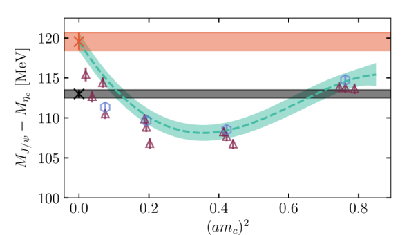
Figure 1: Charmonium hyperfine splitting as a function of lattice spacing. This figure is from [2].

In figure 3.1 we plot the hyperfine splitting as a function of lattice spacing, the blue hexagons and violet triangles showing our results on different ensembles in pure QCD and in QCD+QED respectively. Our extrapolation to the continuum and to physical quark masses is shown by the turquoise error band. The red error band gives our physical result, and the black cross and the black error band show the average experimental result from Particle Data Group [10]. Our final QCD+QED result for the charmonium hyperfine splitting is $M_{J/\psi}-M_{\eta_{c}}=120.3(1.1)\mathrm{\leavevmode\nobreak\ MeV}$.

For the first time we see a significant, 6$\sigma$ difference between the experimental average and a lattice calculation. Note that quark-line disconnected correlation functions are not included in the lattice calculation. The difference between our result and the experimental result is then taken to be the effect of the $\eta_{c}$ decay to two gluons (prohibited in the lattice calculation): $\Delta M_{\eta_{c}}^{\textrm{annihln}}=+7.3(1.2)\mathrm{\leavevmode\nobreak\ MeV}$.

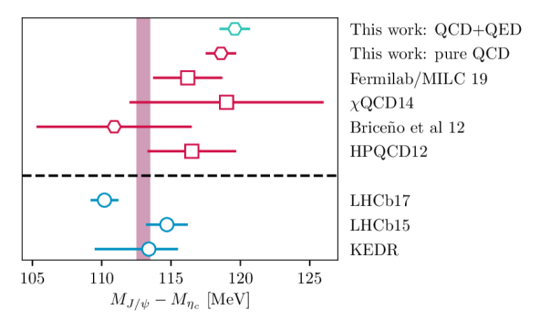
Figure 2: Charmonium hyperfine splitting. This figure is from [2].

In figure 3.1 we compare our result for $M_{J/\psi}-M_{\eta_{c}}$ with other lattice QCD results as well as with experimental results that measure this difference. The results are from the following piblications: Fermilab/MILC [11], $\chi$QCD [12], Briceno [13], HPQCD [14], LHCb [15, 16] and KEDR [17]. The PDG average, shown as the purple error band, is obtained from taking the differences of the PDG $J/\psi$ and $\eta_{c}$ masses rather than only from experiments that directly measure the splitting.

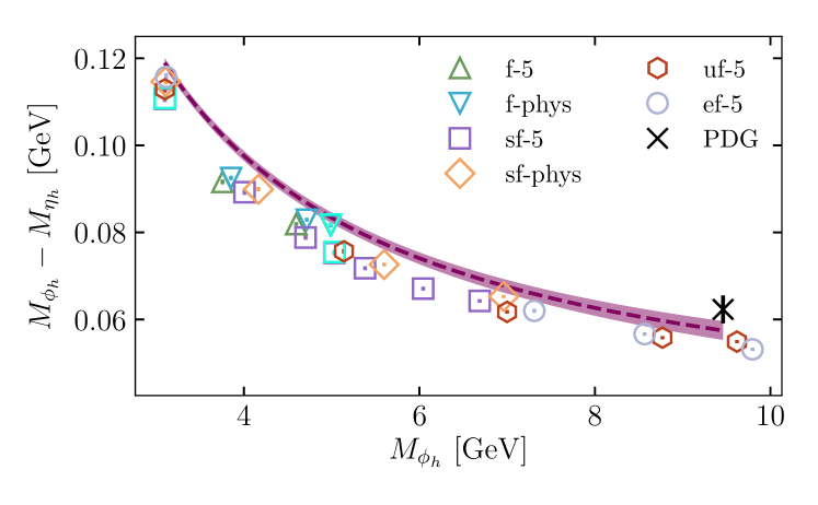
Figure 3: Bottomonium hyperfine splitting. This figure is from [4].

To study the bottomonium hyperfine splitting, we map out the dependence in $m_{h}$ to extract the result at physical $m_{b}$. This is illustrated in figure 3.1, where we plot our results on different lattice ensembles as a function of the heavy vector meson mass $M_{\phi_{h}}$ (which is a proxy for the heavy quark mass). The error band shows the extrapolation to the continuum, and the black cross shows the experimental average from Particle Data Group [18].

Our QCD+QED result for bottomonium hyperfine splitting is $M_{\Upsilon}-M_{\eta_{b}}=57.5(2.3)(1.0)\mathrm{\leavevmode\nobreak\ MeV}$. The missing quark-line disconnected contributions (allowed for by the second uncertainty) are expected to be smaller for bottomonium than charmonium, and here we find good agreement with experiment.

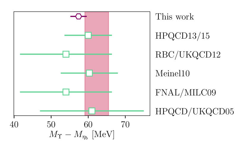
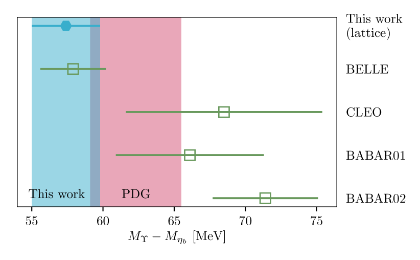
Figure 4: Bottomonium hyperfine splitting. These figures are from [4].

We compare our results to other lattice QCD results and experimental results in figure 3.1. These results are from the following publications: lattice calculations by HPQCD/UKQCD [19], Fermilab/MILC [20], Meinel [21], RBC/UKQCD [22] and HPQCD [23], and experimental results from Belle [24], CLEO [25] and BaBar [26, 27] as well as the experimental average from Particle Data Group [18]. All lattice calculations show good agreement, but there is some tension between the different experimental results with our value favouring (but not significantly) the most recent lower result from Belle.

3.2 Decay constants

The decay constant of a pseudoscalar meson $P$ (e.g. $\eta_{c}$ or $\eta_{b}$) is defined in terms of the axial current as

$$\langle 0|A_{\alpha}|P\rangle=p_{\alpha}f_{P}.$$ (3)

Using the PCAC relation this can be written as

$$\langle 0|\bar{\Psi}_{q}\gamma_{5}\Psi_{q}|P\rangle=\frac{(M_{0}^{P})^{2}}{2m_{q}}f_{P}.$$ (4)

For a vector meson (e.g. $J/\psi$ or $\Upsilon$) the vector decay constant is defined through the vector current

$$\langle 0|\bar{\Psi}_{q}\gamma_{\alpha}\Psi_{q}|V\rangle=f_{V}M_{V}\epsilon_{\alpha},$$ (5)

where $\epsilon$ is the polarisation vector of the meson.

The tensor decay constant of the vector meson is

$$\langle 0|\bar{\Psi}_{q}\sigma_{\alpha\beta}\Psi_{q}|V\rangle=if^{T}_{V}(\mu)(\epsilon_{\alpha}p_{\beta}-\epsilon_{\beta}p_{\alpha}).$$ (6)

Note that the tensor decay constant is scale- and scheme-dependent, unlike the vector decay constant $f_{V}$.

The decay constants can be written in terms of meson masses and amplitudes — see Eq. (2) along with

$$f_{T}=Z_{T}\sqrt{\frac{2A_{0}^{T}}{M_{0}^{V}}},$$ (7)

using amplitudes from a tensor-tensor correlation function.

Our results for the charmonium pseudoscalar and vector decay constants $f_{\eta_{c}}$ and $f_{J/\psi}$ on different lattice ensembles are plotted as a function of the lattice spacing in figure 3.2. The error band shows our extrapolation to the physical point. For $f_{\eta_{c}}$, the black cross shows the result from an earlier lattice calculation by the HPQCD collaboration [28], whereas for $f_{J/\psi}$ the black cross shows the result determined from the experimental average for $\Gamma(J/\psi\to e^{+}e^{-})$. Our QCD+QED results at the physical point are [2] $f_{J/\psi}=410.4(1.7)\mathrm{\leavevmode\nobreak\ MeV}$, $f_{\eta_{c}}=398.1(1.0)\mathrm{\leavevmode\nobreak\ MeV}$ and $f_{J/\psi}/f_{\eta_{c}}=1.0284(19)$.

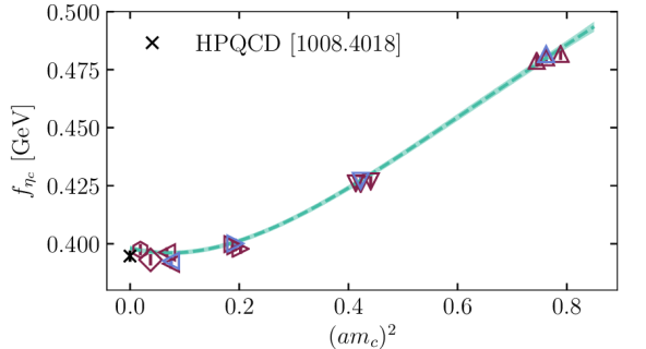
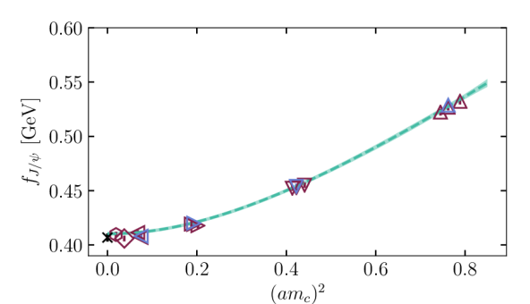
Figure 5: Charmonium decay constants. These figures are from [2].

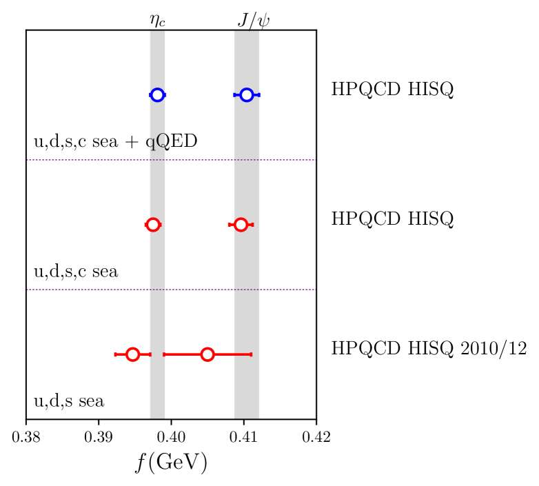
Figure 6: Charmonium decay constants.

The decay constants from the QCD+QED calculation are compared with the pure QCD results in figure 3.2. The QED effects are very small, but at this precision they have to be taken into account. Figure 3.2 also compares these new results to an earlier lattice calculation by the HPQCD collaboration that had only $u$, $d$ and $s$ quarks in the sea [14, 28]. The improvement in the precision highlights how far lattice calculations have come.

Figure 7: Bottomonium decay constants. These figures are from [4].

For bottomonium, we map the dependence of the pseudoscalar decay constant $f_{\eta_{h}}$ and the vector decay constant $f_{\phi_{h}}$ on the heavy quark mass, and extrapolate to the continuum and physical masses in the same way as for the hyperfine splitting. This is illustrated in figure 3.2, that shows lattice results from individual ensembles as well as the extrapolation for both decay constants as a function of the vector meson mass $M_{\phi_{h}}$. The results at the physical point are [4] $f_{\Upsilon}=677.2(9.7)\mathrm{\leavevmode\nobreak\ MeV}$, $f_{\eta_{b}}=724(12)\mathrm{\leavevmode\nobreak\ MeV}$, and $f_{\Upsilon}/f_{\eta_{b}}=0.9454(99)$. For charm the ratio $f_{J/\psi}/f_{\eta_{c}}$ is greater than 1, but for $b$ quarks this is now shown to be $<1$.

As we briefly mentioned earlier, the partial decay width of a vector meson to a lepton pair is directly related to the decay constant:

$$\Gamma(\phi_{h}\to l^{+}l^{-})=\frac{4\pi}{3}\alpha^{2}_{\textrm{QED}}Q^{2}\frac{f^{2}_{\phi_{h}}}{M_{\phi_{h}}},$$ (8)

where $Q$ is the electric charge of the quark. We can thus use our results for the vector decay constants to calculate leptonic widths and compare with experiments, or vice versa.

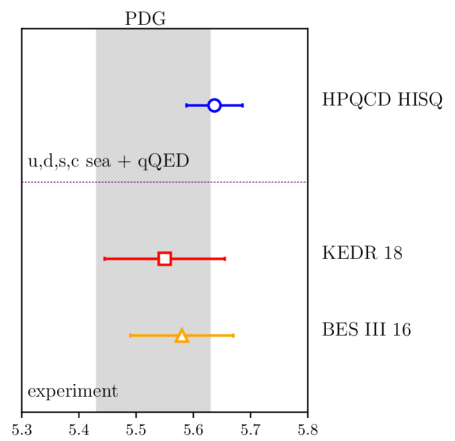
Figure 8: Leptonic width $\Gamma(J/\psi\to e^{+}e^{-})$ [keV] (from [2]).

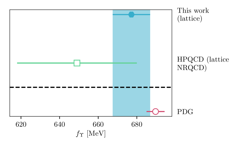
Figure 9: Bottomonium decay constant — comparing lattice QCD (top result) with that inferred from experiment for $\Gamma(\Upsilon\to e^{+}e^{-})$ (bottom result). This figure is from [4].

Our results are: $\Gamma(J/\psi\to e^{+}e^{-})=5.637(47)(13)\mathrm{\leavevmode\nobreak\ keV}$ and $\Gamma(\Upsilon\to e^{+}e^{-})=1.292(37)(3)\mathrm{\leavevmode\nobreak\ keV}$, and we show the comparison with experiment in figures 3.2 (charmonium) and 3.2 (bottomonium). The agreement is seen to be good, and the result from lattice for $\Gamma(J/\psi\to e^{+}e^{-})$ is now more precise than the experimental average from Particle Data Group. There is no experimental decay rate that can be directly compared with the pseudoscalar decay constant.

We now turn to determining the $J/\psi$ tensor decay constant $f^{T}_{J/\psi}$. Recall that the tensor decay constant is scale and scheme dependent, unlike the pseudoscalar and vector decay constants. The calculation (published in [3]) can be summarised as follows:

1. Extract $\sqrt{2A_{0}^{T}/M_{0}^{T}}$ from tensor-tensor correlators.

2. Calculate the renormalisation factor $Z_{T}^{\textrm{SMOM}}$. Convert $f^{T}$ to the $\overline{MS}$ scheme at multiple scales $\mu$ using the RI-SMOM scheme as an intermediate scheme on each ensemble.

3. Run all the $\overline{MS}$ tensor decay constants at a range of scales $\mu$ to a reference scale of $2\textrm{ GeV}$ using a three-loop calculation of the tensor current anomalous dimension. Here $\mu=2,3,4$ GeV.

4. Fit all of the results for the $\overline{MS}$ decay constant at $2\textrm{ GeV}$ to a function that allows for discretisation effects and non-perturbative condensate contamination coming from $Z_{T}^{\textrm{SMOM}}$.

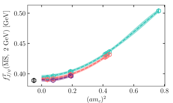
Figure 10: Tensor decay constant $f^{T}_{J/\psi}$. This figure is from [3].

The continuum extrapolation is illustrated in figure 3.2. We plot the tensor decay constant in the $\overline{MS}$ scheme at a scale of 2 GeV using lattice tensor current renormalisation in the RI-SMOM scheme at multiple $\mu$ values. These three values are shown as different coloured lines. The blue line is 2 GeV, the orange, 3 GeV and the purple, 4 GeV. The black hexagon is the physical result for $f^{T}_{J/\psi}(2\textrm{ GeV})$ obtained from the fit (with the condensate contamination removed).

In addition to the tensor decay constant $f^{T}_{J/\psi}(2\textrm{ GeV})$, we also determine the ratio of the tensor and vector decay constants, $f^{T}_{J/\psi}/f^{V}_{J/\psi}$. The extrapolation of the ratio to continuum is illustrated in figure 3.2. The colour coding for the lines and data points is the same as in figure 3.2.

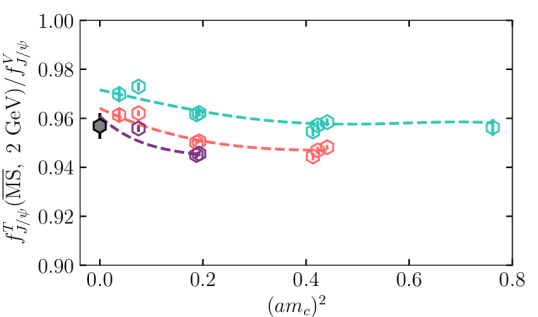
Figure 11: The ratio of tensor and vector decay constants. This figure is from [3].

Our (pure QCD) results for the $J/\psi$ tensor decay constant and its ratio with the vector decay constant are [3] $f^{T}_{J/\psi}(\overline{MS},2\,\mathrm{GeV})=0.3927(27)\mathrm{\leavevmode\nobreak\ GeV}$ and $f^{T}_{J/\psi}(\overline{MS},2\,\mathrm{GeV})/f^{V}_{J/\psi}=0.9569(52)$. The ratio is compared to other lattice QCD and QCD sum rule calculations [29] in figure 3.2. Our result for the ratio is slightly (but not significantly) lower than other results. The new determination of $f^{T}_{J/\psi}$ is much more precise than the previous determinations. This is potentially useful for tests of BSM physics.

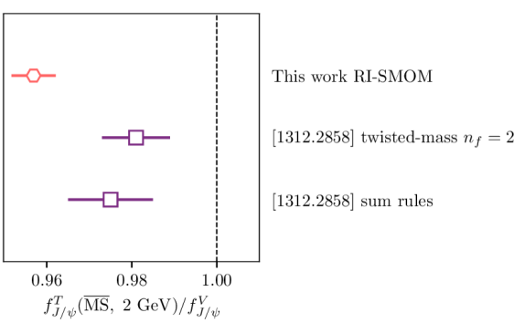
Figure 12: Comparison of the ratio of tensor and vector decay constants.. This figure is from [3].

HPQCD’s results show the high precision achievable now for the properties of ground-state heavyonium mesons. In future this precision will be extended up the spectrum to excited states.

4 Acknowledgements

Computing was done on the Darwin supercomputer and on the Cambridge service for Data Driven Discovery (CSD3), part of which is operated by the University of Cambridge Research Computing on behalf of the DIRAC HPC Facility of the Science and Technology Facilities Council (STFC). The DIRAC component of CSD3 was funded by BEIS capital funding via STFC capital grants ST/P002307/1 and ST/R002452/1 and STFC operations grant ST/R00689X/1. DiRAC is part of the national e-infrastructure. We are grateful to the support staff for assistance. AL acknowledges support by the U.S. Department of Energy under grant number DE-SC0015655.

References

- . C. T. H. Davies et al. (HPQCD, UKQCD, MILC and Fermilab Lattice collaborations), High precision lattice QCD confronts experiment, Phys. Rev. Lett. 92 (2004) 022001, doi:10.1103/PhysRevLett.92.022001, [arXiv:hep-lat/0304004 [hep-lat]].
- . D. Hatton, C. T. H. Davies, B. Galloway, J. Koponen, G. P. Lepage and A. T. Lytle (HPQCD Collaboration), Charmonium properties from lattice QCD+QED: Hyperfine splitting, leptonic width, charm quark mass, and , Phys. Rev. D 102 (2020) 054511, doi:10.1103/PhysRevD.102.054511, [arXiv:2005.01845 [hep-lat]].
- . D. Hatton, C. T. H. Davies, G. P. Lepage and A. T. Lytle (HPQCD Collaboration), Renormalization of the tensor current in lattice QCD and the tensor decay constant, Phys. Rev. D 102 (2020) 094509, doi:10.1103/PhysRevD.102.094509, [arXiv:2008.02024 [hep-lat]].
- . D. Hatton, C. T. H. Davies, J. Koponen, G. P. Lepage and A. T. Lytle (HPQCD Collaboration), Bottomonium precision tests from full lattice QCD: Hyperfine splitting, leptonic width, and quark contribution to hadrons, Phys. Rev. D 103 (2021) 054512, doi:10.1103/PhysRevD.103.054512, [arXiv:2101.08103 [hep-lat]].
- . A. Bazavov et al. (MILC Collaboration), Lattice QCD Ensembles with Four Flavors of Highly Improved Staggered Quarks, Phys. Rev. D 87 (2013) 054505, doi:10.1103/PhysRevD.87.054505, [arXiv:1212.4768 [hep-lat]].
- . A. Bazavov et al. (Fermilab and MILC collaborations), - and -meson leptonic decay constants from four-flavor lattice QCD, Phys. Rev. D 98 (2018) 074512, doi:10.1103/PhysRevD.98.074512, [arXiv:1712.09262 [hep-lat]].
- . E. Follana et al. (HPQCD and UKQCD collaorations), Highly improved staggered quarks on the lattice, with applications to charm physics, Phys. Rev. D 75 (2007) 054502, doi:10.1103/PhysRevD.75.054502, [arXiv:hep-lat/0610092 [hep-lat]].
- . C. McNeile, C. T. H. Davies, E. Follana, K. Hornbostel and G. P. Lepage, High-Precision and HQET from Relativistic Lattice QCD, Phys. Rev. D 85 (2012) 031503, doi:10.1103/PhysRevD.85.031503, [arXiv:1110.4510 [hep-lat]].
- . D. Hatton et al. (HPQCD Collaboration), Renormalizing vector currents in lattice QCD using momentum-subtraction schemes, Phys. Rev. D 100 (2019) 114513, doi:10.1103/PhysRevD.100.114513, [arXiv:1909.00756 [hep-lat]].
- . M. Tanabashi et al. (Particle Data Group), Review of Particle Physics, doi.org/10.1103/PhysRevD.98.030001, Phys. Rev. D 98 (2018) 030001.
- . C. DeTar et al. (Fermilab Lattice and MILC collaborations), Splittings of low-lying charmonium masses at the physical point, Phys. Rev. D 99 (2019) 034509, doi:10.1103/PhysRevD.99.034509, [arXiv:1810.09983 [hep-lat]].
- . Y. B. Yang et al., Charm and strange quark masses and from overlap fermions, Phys. Rev. D 92 (2015) 034517, doi:10.1103/PhysRevD.92.034517, [arXiv:1410.3343 [hep-lat]].
- . R. A. Briceno, H. W. Lin and D. R. Bolton, Charmed-Baryon Spectroscopy from Lattice QCD with = 2+1+1 Flavors, Phys. Rev. D 86 (2012) 094504, doi:10.1103/PhysRevD.86.094504, [arXiv:1207.3536 [hep-lat]].
- . G. C. Donald, C. T. H. Davies, R. J. Dowdall, E. Follana, K. Hornbostel, J. Koponen, G. P. Lepage and C. McNeile (HPQCD Collaboration), Precision tests of the from full lattice QCD: mass, leptonic width and radiative decay rate to , Phys. Rev. D 86 (2012) 094501, doi:10.1103/PhysRevD.86.094501, [arXiv:1208.2855 [hep-lat]].
- . R. Aaij et al. (LHCb), Measurement of the production cross-section in proton-proton collisions via the decay , Eur. Phys. J. C 75 (2015) 311, doi:10.1140/epjc/s10052-015-3502-x, [arXiv:1409.3612 [hep-ex]].
- . R. Aaij et al. [LHCb], Observation of and search for decays, Phys. Lett. B 769 (2017) 305, doi:10.1016/j.physletb.2017.03.046 [arXiv:1607.06446 [hep-ex]].
- . V. V. Anashin et al. (KEDR), Measurement of decay rate and parameters at KEDR, Phys. Lett. B 738 (2014) 391, doi:10.1016/j.physletb.2014.09.064, [arXiv:1406.7644 [hep-ex]].
- . P. Zyla et al. (Particle Data Group), Review of Particle Physics, PTEP 2020 (2020) 083C01, doi.org/10.1093/ptep/ptaa104.
- . A. Gray, I. Allison, C. T. H. Davies, E. Dalgic, G. P. Lepage, J. Shigemitsu and M. Wingate (HPQCD and UKQCD collaborations), The spectrum and from full lattice QCD, Phys. Rev. D 72 (2005) 094507, doi:10.1103/PhysRevD.72.094507, [arXiv:hep-lat/0507013 [hep-lat]].
- . T. Burch, C. DeTar, M. Di Pierro, A. X. El-Khadra, E. D. Freeland, S. Gottlieb, A. S. Kronfeld, L. Levkova, P. B. Mackenzie and J. N. Simone (Fermilab Lattice and MILC collaborations), Quarkonium mass splittings in three-flavor lattice QCD, Phys. Rev. D 81 (2010) 034508, doi:10.1103/PhysRevD.81.034508, [arXiv:0912.2701 [hep-lat]].
- . S. Meinel, Bottomonium spectrum at order from domain-wall lattice QCD: Precise results for hyperfine splittings, Phys. Rev. D 82 (2010) 114502, doi:10.1103/PhysRevD.82.114502, [arXiv:1007.3966 [hep-lat]].
- . Y. Aoki et al. (RBC and UKQCD collaborations), Nonperturbative tuning of an improved relativistic heavy-quark action with application to bottom spectroscopy, Phys. Rev. D 86 (2012) 116003, doi:10.1103/PhysRevD.86.116003, [arXiv:1206.2554 [hep-lat]].
- . R. J. Dowdall et al. (HPQCD collaboration), Bottomonium hyperfine splittings from lattice nonrelativistic QCD including radiative and relativistic corrections, Phys. Rev. D 89 (2014) 031502, [erratum: Phys. Rev. D 92 (2015) 039904], doi:10.1103/PhysRevD.89.031502, [arXiv:1309.5797 [hep-lat]].
- . R. Mizuk et al. (Belle), Evidence for the and observation of and , Phys. Rev. Lett. 109 (2012) 232002, doi:10.1103/PhysRevLett.109.232002, [arXiv:1205.6351 [hep-ex]].
- . G. Bonvicini et al. (CLEO), Measurement of the eta(b)(1S) mass and the branching fraction for Upsilon(3S) — gamma eta(b)(1S), Phys. Rev. D 81 (2010) 031104, doi:10.1103/PhysRevD.81.031104, [arXiv:0909.5474 [hep-ex]].
- . B. Aubert et al. (BaBar), Evidence for the eta(b)(1S) Meson in Radiative Upsilon(2S) Decay, Phys. Rev. Lett. 103 (2009) 161801, doi:10.1103/PhysRevLett.103.161801, [arXiv:0903.1124 [hep-ex]].
- . B. Aubert et al. (BaBar), Observation of the bottomonium ground state in the decay , Phys. Rev. Lett. 101 (2008) 071801, [erratum: Phys. Rev. Lett. 102 (2009) 029901], doi:10.1103/PhysRevLett.101.071801, [arXiv:0807.1086 [hep-ex]].
- . C. T. H. Davies, C. McNeile, E. Follana, G. P. Lepage, H. Na and J. Shigemitsu (HPQCD collaboration), Update: Precision decay constant from full lattice QCD using very fine lattices, Phys. Rev. D 82 (2010) 114504, doi:10.1103/PhysRevD.82.114504, [arXiv:1008.4018 [hep-lat]].
- . D. Bečirević, G. Duplančić, B. Klajn, B. Melić and F. Sanfilippo, Lattice QCD and QCD sum rule determination of the decay constants of , J/ and states, Nucl. Phys. B 883 (2014) 306, doi:10.1016/j.nuclphysb.2014.03.024, [arXiv:1312.2858 [hep-ph]].
- . V. V. Braguta, The study of leading twist light cone wave functions of J/psi meson, Phys. Rev. D 75 (2007) 094016, doi:10.1103/PhysRevD.75.094016, [arXiv:hep-ph/0701234 [hep-ph]].