Scalable global state synchronization of discrete-time double integrator multi-agent systems with input saturation via linear protocol

Abstract

This paper studies scalable global state synchronization of discrete-time double integrator multi-agent systems in presence of input saturation based on localized information exchange. A scale-free collaborative linear dynamic protocols design methodology is developed for discrete-time multi-agent systems with both full and partial-state couplings. And the protocol design methodology does not need any knowledge of the directed network topology and the spectrum of the associated Laplacian matrix. Meanwhile, the protocols are parametric based on a parameter set in which the designed protocols can guarantee the global synchronization result. Furthermore, the proposed protocol is scalable and achieves synchronization for any arbitrary number of agents.

1 Introduction

In recent years, the synchronization or consensus problem of multi-agent system (MAS) has attracted much more attention, due to its wide potential for applications in several areas such as automotive vehicle control, satellites/robots formation, sensor networks, and so on. See for instance the books [1, 2, 11, 22, 26, 27, 38] and references therein.

At present, most work in synchronization for MAS focused on state synchronization of continuous-time and discrete-time homogeneous networks. State synchronization based on diffusive full-state coupling (it means that all states are communicated over the network) has been studied where the agent dynamics progress from single- and double-integrator (e.g. [6, 9, 12, 23, 24, 25, 34]) to more general dynamics (e.g. [33, 37, 40]). State synchronization based on diffusive partial-state coupling (i.e., only part of the states are communicated over the network) has also been considered, including static design ([3, 19, 20]), dynamic design ([10, 17, 29, 32, 35, 36]), and the design with additional communication ([4, 14, 28]).

On the other hand, it is worth to note that actuator saturation is pretty common and indeed is ubiquitous in engineering applications. Some researchers have tried to establish (semi) global state and output synchronization results for both continuous- and discrete-time MAS in the presence of input saturation. From the existing literature for a linear system subject to actuator saturation, we have the following conclusion [27]:

1. A linear protocol is used if we consider synchronization in the semi-global framework (i.e. initial conditions of agents are in a priori given compact set).

2. Synchronization in the global sense (i.e., when initial conditions of agents are anywhere) in general requires a nonlinear protocol.

3. Synchronization in the presence of actuator saturation requires eigenvalues of agents to be in the closed left half plane for continuous-time systems and in the closed unit disc for discrete-time systems, that is the agents are at most weakly unstable.

The semi-global synchronization has been studied in [31] via full-state coupling. For partial state coupling, we have [30, 41] which are based on the extra communication. Meanwhile, the result without the extra communication is developed in [42]. Then, the static controllers via partial state coupling is designed in [16] by passifying the original agent model.

On the other hand, global synchronization for full-state coupling has been studied by [21] (continuous-time) and [39] (discrete-time) for neutrally stable and double-integrator agents. The global framework has only been studied for static protocols under the assumption that the agents are neutrally stable and the network is detailed balanced or undirected. Partial-state coupling has been studied in [5] using an adaptive approach but the observer requires extra communication. The result dealing with networks that are not detailed balanced are based on [13] which intrinsically requires the agents to be single integrators. Recently, we introduce a scale-free linear collaborative protocols for global regulated state synchronization of continuous- and discrete-time homogeneous MAS, see [18] and [15]. This scale-free protocol means the design is independent of the information about the associated communication graph or the size of the network, i.e., the number of agents.

In this paper, we focus on scalable linear protocol design for global state synchronization of discrete-time double-integrator MAS in presence of input saturation. The contributions of this paper are stated as follows:

• A class of parametric linear protocol is established based on a parameter set in which the designed parametric protocol makes all states of MAS synchronized.

• Meanwhile, the linear protocol design is scale-free and do not need any information about communication network. In other words, the proposed protocols work for any MAS with any communication graph with arbitrary number of agents as long as the communication graph has a path among each agent.

Notations and definitions

Given a matrix $A\in\mathbb{R}^{m\times n}$, $A^{\mbox{\tiny T}}$ denotes its conjugate transpose and $\|A\|$ is the induced 2-norm. A square matrix $A$ is said to be Schur stable if all its eigenvalues are in the closed unit disk. $A\otimes B$ depicts the Kronecker product between $A$ and $B$. $I_{n}$ denotes the $n$-dimensional identity matrix and $0_{n}$ denotes $n\times n$ zero matrix; sometimes we drop the subscript if the dimension is clear from the context. A matrix $D=[d_{ij}]_{N\times N}$ is called a row stochastic matrix if (a) $d_{ij}>0$ for any $i,j$ and (b) $\sum_{j}^{N}d_{ij}=1$ for $i=1,\cdots,N$. A row stochastic matrix $D$ has at least one eigenvalue at 1 with right eigenvector 1.

A weighted graph $\mathcal{G}$ is defined by a triple $(\mathcal{V},\mathcal{E},\mathcal{A})$ where $\mathcal{V}=\{1,\ldots,N\}$ is a node set, $\mathcal{E}$ is a set of pairs of nodes indicating connections among nodes, and $\mathcal{A}=[a_{ij}]\in\mathbb{R}^{N\times N}$ is the weighting matrix. Each pair in $\mathcal{E}$ is called an edge, where $a_{ij}>0$ denotes an edge $(j,i)\in\mathcal{E}$ from node $j$ to node $i$ with weight $a_{ij}$. Moreover, $a_{ij}=0$ if there is no edge from node $j$ to node $i$. We assume there are no self-loops, i.e. we have $a_{ii}=0$. A path from node $i_{1}$ to $i_{k}$ is a sequence of nodes $\{i_{1},\ldots,i_{k}\}$ such that $(i_{j},i_{j+1})\in\mathcal{E}$ for $j=1,\ldots,k-1$. A directed tree with root $r$ is a subgraph of the graph $\mathcal{G}$ in which there exists a unique path from node $r$ to each node in this subgraph. A directed spanning tree is a directed tree containing all the nodes of the graph. A directed graph may contain many directed spanning trees, and thus there may be several choices for the root agent. The set of all possible root agents for a graph $\mathcal{G}$ is denoted by $\pi_{g}$.

The weighted in-degree of node $i$ is given by

$$d_{\text{in}}(i)=\sum_{j=1}^{N}\,a_{ij}.$$

For a weighted graph $\mathcal{G}$, the matrix $L=[\ell_{ij}]$ with

$$\ell_{ij}=\left\{\;\begin{array}[]{cl}\sum_{k=1}^{N}a_{ik},&i=j,\\ -a_{ij},&i\neq j,\end{array}\right.$$

is called the Laplacian matrix associated with the graph $\mathcal{G}$. The Laplacian matrix $L$ has all its eigenvalues in the closed right half plane and at least one eigenvalue at zero associated with right eigenvector 1 [7].

2 Problem formulation

Consider a MAS consisting of $N$ identical discrete-time double integrator with input saturation:

$$\begin{cases}{x}_{i}(k+1)=Ax_{i}(k)+B\sigma(u_{i}(k)),\\ y_{i}(k)=Cx_{i}(k)\end{cases}$$ (1)

where $x_{i}(k)\in\mathbb{R}^{2n}$, $y_{i}(k)\in\mathbb{R}^{n}$ and $u_{i}(k)\in\mathbb{R}^{n}$ are the state, output, and the input of agent $i=1,\ldots,N$, respectively. And

$$A=\begin{pmatrix}I&I\\ 0&I\end{pmatrix},B=\begin{pmatrix}0\\ I\end{pmatrix},C=\begin{pmatrix}I&0\end{pmatrix}$$

Meanwhile,

$$\sigma(v)=\begin{pmatrix}\operatorname{sat}(v_{1})\\ \operatorname{sat}(v_{2})\\ \vdots\\ \operatorname{sat}(v_{m})\end{pmatrix}\quad\text{ where }\quad v=\begin{pmatrix}v_{1}\\ v_{2}\\ \vdots\\ v_{m}\end{pmatrix}\in\mathbb{R}^{m}$$

with $\operatorname{sat}(w)$ is the standard saturation function,

$$\operatorname{sat}(w)=\operatorname{sgn}(w)\min(1,|w|).$$

The network provides agent $i$ with the following information,

$$\zeta_{i}(k)=\sum_{j=1}^{N}a_{ij}(y_{i}(k)-y_{j}(k)),$$ (2)

where $a_{ij}\geqslant 0$ and $a_{ii}=0$. This communication topology of the network can be described by a weighted graph $\mathcal{G}$ associated with (2), with the $a_{ij}$ being the coefficients of the weighting matrix $\mathcal{A}$. In terms of the coefficients of the associated Laplacian matrix $L$, $\zeta_{i}$ can be rewritten as

$$\zeta_{i}(k)=\sum_{j=1}^{N}\ell_{ij}y_{j}(k).$$ (3)

We refer to this as partial-state coupling since only part of the states are communicated over the network. When $C=I$, it means all states are communicated over the network, we call it full-state coupling. Then, the original agents are expressed as

$${x}_{i}(k+1)=Ax_{i}(k)+B\sigma(u_{i}(k))$$ (4)

and $\zeta_{i}$ is rewritten as

$$\zeta_{i}(k)=\sum_{j=1}^{N}\ell_{ij}x_{j}(k).$$ (5)

We need the following definition to explicitly state our problem formulation.

Definition 1

We define the following set. $\mathbb{G}^{N}$ denotes the set of directed graphs of $N$ agents which contains a directed spanning tree. Moreover, for any $\mathcal{G}\in\mathbb{G}^{N}$, we denote the root set of the $\mathcal{G}$ by $\pi_{g}$.

Remark 1

When the undirected or strongly connected graph is considered, it is obvious that the set $\pi_{g}$ will include all nodes of networks.

We consider the state synchronization problem under the graph set $\mathbb{G}^{N}$ satisfying Definition 1. Here, its objective is that the agents achieve state synchronization, that is

$$\lim_{k\to\infty}(x_{i}(k)-x_{j}(k))=0.$$ (6)

for all $i,j\in{1,...,N}$.

Meanwhile, we introduce an additional information exchange among each agent and its neighbors. In particular, each agent $i=1,\ldots,N$ has access to additional information, denoted by $\hat{\zeta}_{i}$, of the form

$$\hat{\zeta}_{i}(k)=\sum_{j=1}^{N}a_{ij}(\xi_{i}(k)-\xi_{j}(k))$$ (7)

where $\xi_{j}\in\mathbb{R}^{n}$ is a variable produced internally by agent $j$ and to be defined in next sections.

Then, we formulate the problem for global state synchronization of a MAS via linear protocols based on additional information exchange (7).

Problem 1

Consider a MAS described by (1) and (2). Let the set $\mathbb{G}^{N}$ denote all graphs satisfy Definition 1.

The scalable global state synchronization problem with additional information exchange via linear dynamic protocol is to find a linear dynamic protocol, using only the knowledge of agent model $(A,B,C)$, of the form

$$\left\{\;\begin{array}[]{cl}x_{c,i}(k+1)=&A_{c,i}x_{c,i}(k)+B_{c,i}{\sigma(u_{i}(k))}\\ &\hskip 42.67912pt+C_{c,i}{\zeta}_{i}(k)+D_{c,i}\hat{\zeta}_{i}(k),\\ u_{i}(k)=&K_{c,i}x_{c,i}(k)\end{array}\right.$$ (8)

where $\hat{\zeta}_{i}$ is defined in (7) with $\xi_{i}=H_{c,i}x_{c,i}$, and $x_{c,i}\in\mathbb{R}^{n_{c}}$, such that state synchronization (6) is achieved for any $N$ and any graph $\mathcal{G}\in\mathbb{G}^{N}$, and for all initial conditions of the agents $x_{i}(0)\in\mathbb{R}^{n}$, and all initial conditions of the protocols $x_{c,i}(0)\in\mathbb{R}^{n_{c}}$.

3 Protocol design

3.1 Full-state coupling

Let $\mathcal{G}$ be any graph belongs to $\mathbb{G}^{N}$, and we choose agent $\theta$ where $\theta$ is any node in the root set $\pi_{g}$. Then, we propose the following protocol.

Linear Protocol 1: Full-state coupling

$$\left\{\;\begin{array}[]{cll}{\chi}_{i}(k+1)&=&A\chi_{i}(k)+B\sigma(u_{i}(k))\\ &&\quad+\frac{1}{1+D_{in}(i)}\left[A{\zeta}_{i}(k)-A\hat{\zeta}_{i}(k)\right]\\ u_{i}(k)&=&K\chi_{i}(k),\quad i=\{1,\ldots,N\}\setminus\theta\\ u_{\theta}(k)&\equiv&0,\end{array}\right.$$ (9) where $D_{\text{in}}(i)$ is the upper bound of $d_{in}(i)=\sum_{j=1}^{N}a_{ij}$. Then, we still choose matrix $K=-\begin{pmatrix}k_{1}I&k_{2}I\end{pmatrix}$, where $k_{1}\in(0,1)$ and $k_{2}>0$ satisfy the following condition $$(1+k_{1}-k_{2})^{2}<1-k_{1}.$$ (10) $\hat{\zeta}_{i}(k)$ and ${\zeta}_{i}(k)$ are defined by (7) and (2), respectively. And the agents communicate $\xi_{i}(k)$ which is chosen as $\xi_{i}(k)=\chi_{i}(k)$.

Remark 2

$D_{\text{in}}(i)$ is an upper bound for the weighted in-degree $d_{\text{in}}(i)=\sum_{j=1}^{N}a_{ij}$ for node $i$. It is still local information. In our protocol design, the bound $D_{\text{in}}(i)$ is used to scale the communication among agents, which can otherwise cancel the impact of the $\theta$th weighting value.

The condition (10) can be shown as Fig. 1, where the zone encircled by parabola and line $(0,0)$ to $(0,2)$.

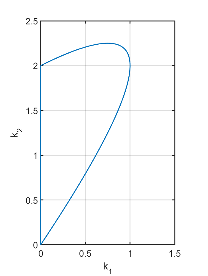
Figure 1: Solvable zone of $k_{1},k_{2}$ for synchronization

Theorem 1

Consider a MAS described by (4) and (5). Let the set $\mathbb{G}^{N}$ denote all graphs satisfy Definition 1.

Then, the scalable global state synchronization problem with additional information exchange as stated in Problem 1 is solvable. In particular, for any given $k_{1}\in(0,1)$ and $k_{2}>0$ satisfying (10), the linear dynamic protocol (9) solves the global state synchronization problem for any $N$ and any graph $\mathcal{G}\in\mathbb{G}^{N}$.

To obtain this theorem we need the following lemma.

Lemma 1

For all $u,v\in\mathbb{R}^{n}$, we have

$$(\sigma(v)-\sigma(u))^{\mbox{\tiny T}}(u-\sigma(u))\leqslant 0.$$ (11)

Proof: Note that we have:

$$(\sigma(v)-\sigma(u))^{\mbox{\tiny T}}(u-\sigma(u))\\ =\sum_{i=1}^{n}(\sigma(v_{i})-\sigma(u_{i}))(u_{i}-\sigma(u_{i}))$$ (12)

when:

$$u=\begin{pmatrix}u_{1}\\ \vdots\\ u_{n}\end{pmatrix},\qquad v=\begin{pmatrix}v_{1}\\ \vdots\\ v_{n}\end{pmatrix}$$

Next note that if $u_{i}\geqslant 1$ we have $\sigma(v_{i})-\sigma(u_{i})=\sigma(v_{i})-1\leqslant 0$ and $u_{i}-\sigma(u_{i})=u_{i}-1\geqslant 0$ and hence:

$$(\sigma(v_{i})-\sigma(u_{i}))(u_{i}-\sigma(u_{i}))\leqslant 0$$ (13)

On the other hand if $u_{i}\leqslant-1$ we have $\sigma(v_{i})-\sigma(u_{i})=\sigma(v_{i})+1\geqslant 0$ and $u_{i}-\sigma(u_{i})=u_{i}+1\leqslant 0$ and (13) is still satisfied. Finally, if $|u_{i}|\leqslant 1$ then $u_{i}-\sigma(u_{i})=0$ and (13) is also satisfied.

Since (13) is satisfied for all $i$ and using (12) we find (11) holds for all $u$ and $v$.  

The proof of Theorem 1:  Since we have $u_{\theta}(k)\equiv 0$, we obtain $\sigma(u_{\theta}(k))=0$. The model of agent $\theta$ is rewritten as

$$x_{\theta}(k+1)=Ax_{\theta}(k)$$

Then, let $\bar{x}(k)=x_{i}(k)-x_{\theta}(k)$, we have

$$\left\{\;\begin{array}[]{l}\bar{x}_{i}(k+1)=A\bar{x}_{i}(k)+B\sigma(u_{i}(k))\\ \chi_{i}(k+1)=A\chi_{i}(k)+B\sigma(u_{i}(k))\\ \qquad\qquad\quad+\frac{1}{1+D_{{in}}(i)}\sum_{j=1}^{N-1}{\ell}_{ij}A\left[\bar{x}_{i}(k)-\chi_{i}(k)\right]\\ u_{i}(k)=-\begin{pmatrix}k_{1}I&k_{2}I\end{pmatrix}\chi_{i}(k)\end{array}\right.$$ (14)

Then by defining $2(N-1)n$-dimensional vectors

$$\bar{x}(k)=\begin{pmatrix}\bar{x}_{1}(k)\\ \vdots\\ \bar{x}_{N-1}(k)\end{pmatrix},{\chi}(k)=\begin{pmatrix}\chi_{1}(k)\\ \vdots\\ \chi_{N}(k)\end{pmatrix},\\ u(k)=\begin{pmatrix}u_{1}(k)\\ \vdots\\ u_{N}(k)\end{pmatrix},\sigma(u(k))=\begin{pmatrix}\sigma(u_{1}(k))\\ \vdots\\ \sigma(u_{N}(k))\end{pmatrix}$$

where $\chi_{\theta}(k)$, $u_{\theta}(k)$, and $\sigma(u_{\theta}(k))$ are not included. We have the following closed-loop system

$$\left\{\;\begin{array}[]{l}\bar{x}(k+1)=(I_{N-1}\otimes A)\bar{x}(k)+(I_{N-1}\otimes B)\sigma(u(k))\\ \chi(k+1)=(I_{N-1}\otimes A)\chi(k)+(I_{N-1}\otimes B)\sigma(u(k))\\ \hskip 56.9055pt+((I_{N-1}-\bar{D})\otimes A)(\bar{x}(k)-\chi(k))\\ u(k)=-(I_{N-1}\otimes\begin{pmatrix}k_{1}I&k_{2}I\end{pmatrix})\chi(k)\end{array}\right.$$ (15)

where $\bar{D}=I_{N-1}-(I_{N-1}+D_{d,\text{in}})^{-1}\hat{L}$,

$$D_{d,\text{in}}=\operatorname{diag}\{D_{in}(1),D_{in}(2),\cdots,D_{in}(N)\}\text{ without }D_{in}(\theta),$$

and $\hat{L}$ is the matrix obtained from $L$ by deleting the $\theta$th row and the $\theta$th column. Meanwhile, according to [8, Lemma 1], we have the real part of all eigenvalues of $\hat{L}$ are greater than zero. Thus, it implies all eigenvalues’ absolute value of $\bar{D}\in\mathbb{R}^{(N-1)\times(N-1)}$ are less than 1.

Let $e(k)=\bar{x}(k)-\chi(k)$, we have

$$\left\{\;\begin{array}[]{l}\bar{x}(k+1)=(I_{N-1}\otimes A)\bar{x}(k)+(I_{N-1}\otimes B)\sigma(u(k))\\ e(k+1)=(\bar{D}\otimes A)e(k)\\ u(k)=-(I_{N-1}\otimes\begin{pmatrix}k_{1}I&k_{2}I\end{pmatrix})(\bar{x}(k)-e(k))\end{array}\right.$$ (16)

Then, let

$$\bar{x}_{i}(k)=\begin{pmatrix}\bar{x}_{1,i}(k)\\ \bar{x}_{2,i}(k)\end{pmatrix},$$

we have

$$\left\{\;\begin{array}[]{l}\bar{x}_{1}(k+1)=\bar{x}_{1}(k)+\bar{x}_{2}(k)\\ \bar{x}_{2}(k+1)=\bar{x}_{2}(k)+\sigma(u(k))\\ e(k+1)=(\bar{D}\otimes A)e(k)\\ u(k)=-k_{1}\bar{x}_{1}(k)-k_{2}\bar{x}_{2}(k)+\left(I_{N-1}\otimes\begin{pmatrix}k_{1}I&k_{2}I\end{pmatrix}\right)e(k)\end{array}\right.$$ (17)

The eigenvalues of $\bar{D}\otimes A$ are of the form $\lambda_{i}\mu_{j}$, with $\lambda_{i}$ and $\mu_{j}$ eigenvalues of $\bar{D}$ and $A$, respectively. Since $|\lambda_{i}|<1$ and $\mu_{j}\equiv 1$, we find $\bar{D}\otimes A$ is asymptotically stable. Therefore we find that:

$$\lim_{k\to\infty}e_{i}(k)\to 0.$$ (18)

It also shows that $e_{i}\in\ell_{2}$. Thus, we just need to prove the stability of (17). Thus, we have $\bar{x}(k)\to 0$ as $k\to\infty$ with $e_{i}\in\ell_{2}$, which will obtain the synchronization result.

To prove the synchronization result, we consider the following weighting Lyapunov function

$$V(k)=(1-h)V_{1}(k)+hV_{2}(k)$$ (19)

where $h\in(0,1)$,

$$V_{1}(k)= \begin{pmatrix}\sigma(u(k))\\ \bar{x}_{2}(k)\end{pmatrix}^{\mbox{\tiny T}}\left[\begin{pmatrix}1&k_{1}\\ k_{1}&{k_{1}}\end{pmatrix}\otimes I_{(N-1)n}\right]\begin{pmatrix}\sigma(u(k))\\ \bar{x}_{2}(k)\end{pmatrix}$$

$$\hskip 56.9055pt+2\sigma(u(k))^{\mbox{\tiny T}}(u(k)-\sigma(u(k)))$$

$$V_{2}(k)= e^{\mbox{\tiny T}}(k)P_{D}e(k)$$

and $P_{D}>0$ satisfies

$$(\bar{D}\otimes A)^{\mbox{\tiny T}}P_{D}(\bar{D}\otimes A)-P_{D}\leqslant-2I_{2(N-1)n}.$$ (20)

Here, we obtain $V_{1}(k)$ and $V_{2}(k)$ are positive, i.e. $V_{1}(k)>0$ except for $(u(k),\bar{x}_{2}(k))=0$ when $V_{1}(k)=0$ and $V_{2}(k)>0$ except for $e(k)=0$ when $V_{2}(k)=0$. Then, we have

$$\Delta V_{1}(k)=V_{1}(k+1)-V_{1}(k)$$

$$= -\sigma(u(k+1))^{\mbox{\tiny T}}\sigma(u(k+1))+2\sigma(u(k+1))^{\mbox{\tiny T}}u(k)$$

$$+2(k_{1}-k_{2})\sigma(u(k+1))^{\mbox{\tiny T}}\sigma(u(k))$$

$$+(1+k_{1})\sigma(u(k))^{\mbox{\tiny T}}\sigma(u(k))-2\sigma(u(k))^{\mbox{\tiny T}}u(k)$$

$$+2\sigma(u(k+1))^{\mbox{\tiny T}}(I_{N-1}\otimes(k_{1}I\quad k_{2}I)\Psi)e(k)$$

$$= 2(\sigma(u(k+1))-\sigma(u(k)))^{\mbox{\tiny T}}(u(k)-\sigma(u(k)))$$

$$+2(1+k_{1}-k_{2})\sigma(u(k+1))^{\mbox{\tiny T}}\sigma(u(k))$$

$$-\sigma(u(k+1))^{\mbox{\tiny T}}\sigma(u(k+1))-(1-k_{1})\sigma(u(k))^{\mbox{\tiny T}}\sigma(u(k))$$

$$+2\sigma(u(k+1))^{\mbox{\tiny T}}(I_{N-1}\otimes(k_{1}I\quad k_{2}I)\Psi)e(k)$$

$$\leqslant 2(1+k_{1}-k_{2})\sigma(u(k+1))^{\mbox{\tiny T}}\sigma(u(k))$$

$$-\sigma(u(k+1))^{\mbox{\tiny T}}\sigma(u(k+1))-(1-k_{1})\sigma(u(k))^{\mbox{\tiny T}}\sigma(u(k))$$

$$+2\sigma(u(k+1))^{\mbox{\tiny T}}(I_{N-1}\otimes(k_{1}I\quad k_{2}I)\Psi)e(k)$$

since $(\sigma(u(k+1))-\sigma(u(k)))^{\mbox{\tiny T}}(u(k)-\sigma(u(k)))\leqslant 0$ based on Lemma 1, where $\Psi=\bar{D}\otimes A-I_{2(N-1)n}$. Meanwhile, for $V_{2}(k)$ we have

$$\Delta V_{2}(k)=V_{2}(k+1)-V_{2}(k)\leqslant-2e^{\mbox{\tiny T}}(k)e(k)$$

based on condition (20). Thus, one can obtain

$$\Delta V(k)\leqslant(1-h)\Delta V_{1}(k)+h\Delta V_{2}(k)$$

$$\leqslant 2(1-h)(1+k_{1}-k_{2})\sigma(u(k+1))^{\mbox{\tiny T}}\sigma(u(k))$$

$$-(1-h)\left(1-\frac{\|\Psi\|^{2}(1-h)(k_{1}^{2}+k_{2}^{2})}{h}\right)$$

$$\times\|\sigma(u(k+1))\|^{2}-(1-h)(1-k_{1})\sigma(u(k))^{\mbox{\tiny T}}\sigma(u(k))$$

$$-he^{\mbox{\tiny T}}(k)e(k)$$

$$= (1-h)\begin{pmatrix}\sigma(u(k+1))\\ \sigma(u(k))\end{pmatrix}^{\mbox{\tiny T}}(\Phi\otimes I_{(N-1)n})\begin{pmatrix}\sigma(u(k+1))\\ \sigma(u(k))\end{pmatrix}$$

$$-he^{\mbox{\tiny T}}(k)e(k)$$

where

$$\Phi=\begin{pmatrix}-1+\frac{\|\Psi\|^{2}(1-h)(k_{1}^{2}+k_{2}^{2})}{h}&1+k_{1}-k_{2}\\ 1+k_{1}-k_{2}&-(1-k_{1})\end{pmatrix}.$$ (21)

Obviously we just need to prove $\Phi<0$. Without loss of generality, there exists an $\varepsilon>0$ such that

$$\frac{(1+k_{1}-k_{2})^{2}}{1-k_{1}}=1-\varepsilon.$$ (22)

By using Schur Compliment, we have $\Phi<0$ is equivalent to

$$-1+\frac{\|\Psi\|^{2}(1-h)(k_{1}^{2}+k_{2}^{2})}{h}+\frac{(1+k_{1}-k_{2})^{2}}{1-k_{1}}<0.$$

From condition (22), we can obtain

$$-1+\frac{\|\Psi\|^{2}(1-h)(k_{1}^{2}+k_{2}^{2})}{h}+\frac{(1+k_{1}-k_{2})^{2}}{1-k_{1}}$$

$$< \frac{\|\Psi\|^{2}(1-h)(k_{1}^{2}+k_{2}^{2})}{h}-\varepsilon$$

For $h$ sufficiently close to 1, one can obtain

$$\frac{\|\Psi\|^{2}(1-h)(k_{1}^{2}+k_{2}^{2})}{h}<\varepsilon$$

It means that we obtain $\Phi<0$.

Thus, we have $\Delta V(k)<0$ for $\begin{pmatrix}\sigma(u(k+1))\\ \sigma(u(k))\end{pmatrix}\neq 0$, $\bar{x}(k)\to 0$ as $k\to\infty$.

Furthermore, when $\Delta V(k)=0$, we obtain $u(k+1)=u(k)=0$ and $e(k)=0$. It is easy to obtain $\bar{x}_{1}(k)=\bar{x}_{2}(k)=0$ at $\Delta V(k)=0$.

Thus, the invariance set $\{(\bar{x}(k),e(k)):\Delta{V}(\bar{x}(k),e(k))=0\}$ contains no trajectory of the system except the trivial trajectory $(\bar{x}(k),e(k))=(0,0)$. (16) is globally asymptotically stable based on LaSalle’s invariance principle.

Finally, we obtain the global state synchronization result.  

Remark 3

From Theorem 1, we can know that the solvable zone shown in Fig. 1 is an open zone, i.e., $\frac{(1+k_{1}-k_{2})^{2}}{1-k_{1}}<1$ and $k_{1}>0$. However, if let $k_{1}=1$ and $k_{2}=2$, then we just need $\frac{\|\Psi\|^{2}(1-h)(k_{1}^{2}+k_{2}^{2})}{h}<1$ to guarantee $\Phi\leqslant 0$. Obviously, it is obtained for some $h\to 1$. Thus, the point $(1,2)$ is also a pair of solvable parameter for scalable synchronization result.

3.1.1 Partial-state coupling

Let $\mathcal{G}$ be any graph belongs to $\mathbb{G}^{N}$, and also we choose agent $\theta$ where $\theta$ is any node in the root set $\pi_{g}$. Then, we propose the following linear protocol.

Linear protocol 2: Partial-state coupling

$$\left\{\;\begin{array}[]{cll}\hat{x}_{i}(k+1)&=&(A-FC)\hat{x}_{i}(k)\\ &&\quad+\frac{1}{1+D_{{in}}(i)}\left[B\hat{\zeta}_{i2}(k)+F{\zeta}_{i}(k)\right]\\ {\chi}_{i}(k+1)&=&A\chi_{i}(k)+Bu_{i}(k)\\ &&\quad+A\hat{x}_{i}(k)-\frac{1}{1+D_{{in}}(i)}A\hat{\zeta}_{i1}(k)\\ u_{i}(k)&=&K\chi_{i}(k),\quad i=\{1,\ldots,N\}\setminus\theta\\ u_{\theta}(k)&\equiv&0,\end{array}\right.$$ (23) where $D_{\text{in}}(i)$ is the upper bound of $d_{in}(i)=\sum_{j=1}^{N}a_{ij}$. Then, we choose matrix $K=-\begin{pmatrix}k_{1}I&k_{2}I\end{pmatrix}$, where $k_{1}\in(0,1),k_{2}>0$ satisfy condition (10). In this protocol, the agents communicate $$\xi_{i}(k)=\begin{pmatrix}\xi_{i1}(k)\\ \xi_{i2}(k)\end{pmatrix}=\begin{pmatrix}\chi_{i}(k)\\ \sigma(u_{i}(k))\end{pmatrix},$$ i.e. each agent has access to additional information $$\hat{\zeta}_{i}(k)=\begin{pmatrix}\hat{\zeta}_{i1}(k)\\ \hat{\zeta}_{i2}(k)\end{pmatrix},$$ where: $$\left\{\;\begin{array}[]{l}\hat{\zeta}_{i1}(k)=\sum_{j=1}^{N}a_{ij}(\chi_{i}(k)-\chi_{j}(k))\\ \hat{\zeta}_{i2}(k)=\sum_{j=1}^{N}a_{ij}(\sigma(u_{i}(k))-\sigma(u_{j}(k)))\end{array}\right.$$ (24) while $\bar{\zeta}_{i}(k)$ is defined via (2).

We have following theorem.

Theorem 2

Consider a MAS described by (1) and (2). Let the set $\mathbb{G}^{N}$ denote all graphs satisfy Definition 1.

Then, the scalable global state synchronization problem with additional information exchange as stated in Problem 1 is solvable. In particular, for any given $k_{1}\in(0,1)$ and $k_{2}>0$ satisfying (10), the linear dynamic protocol (23) solves the global state synchronization problem for any $N$ and any graph $\mathcal{G}\in\mathbb{G}^{N}$.

The proof of Theorem 2:  Similar to Theorem 1, by defining $\bar{x}_{i}(k)=x_{i}(k)-x_{\theta}(k)$, $e(k)=\bar{x}(k)-\chi(k)$, and $\bar{e}(k)=[(I_{N-1}-\bar{D})\otimes I]\bar{x}(k)-\hat{x}(k)$, we have the matrix expression of closed-loop system

$$\left\{\;\begin{array}[]{l}\bar{x}_{1}(k+1)=\bar{x}_{1}(k)+\bar{x}_{2}(k)\\ \bar{x}_{2}(k+1)=\bar{x}_{2}(k)+\sigma(u(k))\\ e(k+1)=(\bar{D}\otimes A)e(k)+\bar{e}(k)\\ \bar{e}(k+1)=[I_{N-1}\otimes(A-FC)]\bar{e}(k)\\ u(k)=-\left(I_{N-1}\otimes\begin{pmatrix}k_{1}I&k_{2}I\end{pmatrix}\right)\chi(k)\end{array}\right.$$

Since the eigenvalues of $A-FC$ and $\bar{D}\otimes A$ are in open unit disk, we just need to prove the stability of $\bar{x}_{1}(k)$ and $\bar{x}_{2}(k)$.

Similar to the proof of Theorem 1, the state synchronization result can be obtained.  

4 Numerical examples

In this section, we will illustrate the effectiveness and scalability of our designs for discrete time double-integrator MAS by one numerical example. We use agent models (1) with parameters

$$A=\begin{pmatrix}1&1\\ 0&1\end{pmatrix},B=\begin{pmatrix}0\\ 1\end{pmatrix},C=\begin{pmatrix}1&0\end{pmatrix}$$

Meanwhile, we use three graphs which consists of 4, 7, and 60 agents respectively. We consider the case of global state synchronization with partial-state coupling. To show the effectiveness of our protocol design based on condition (10), we choose $F=[1.5\quad 0.5]^{\mbox{\tiny T}}$, $k_{1}=0.5$ and $k_{2}=1$. Furthermore, we choose $\theta=1$. The protocol is provided as follows:

$$\left\{\;\begin{array}[]{ll}\hat{x}_{i}(k+1)&=\begin{pmatrix}-0.5&1\\ -0.5&1\end{pmatrix}\hat{x}_{i}(k)\\ &\qquad+\frac{1}{1+D_{\text{in}}(i)}\left[\begin{pmatrix}0\\ 1\end{pmatrix}\hat{\zeta}_{i2}(k)+\begin{pmatrix}1.5\\ 0.5\end{pmatrix}{\zeta}_{i}(k)\right]\\ {\chi}_{i}(k+1)&=\begin{pmatrix}1&1\\ 0&1\end{pmatrix}\left[\chi_{i}(k)-\frac{1}{1+D_{\text{in}}(i)}\hat{\zeta}_{i1}(k)\right]\\ &\qquad+\begin{pmatrix}0\\ 1\end{pmatrix}\sigma(u_{i}(k))+\begin{pmatrix}1&1\\ 0&1\end{pmatrix}\hat{x}_{i}(k)\\ u_{i}(k)&=-\begin{pmatrix}k_{1}&k_{2}\end{pmatrix}\chi_{i}(k).\end{array}\right.$$ (25)

with $i=2,\cdots,N$.

Now we are creating three homogeneous MAS with different number of agents and different communication topologies to show that the designed protocol is scale-free, independent of the communication network, and number of agents $N$.

Case I: 4-agent graph

In this case, we consider a MAS with $4$ agents, $N=4$. The associated adjacency matrix to the communication network is assumed to be $\mathcal{A}_{I}$ where $a_{21}=a_{32}=a_{43}=1$.

The simulation results of Case I by using protocol (25) are demonstrated in Figure 2.

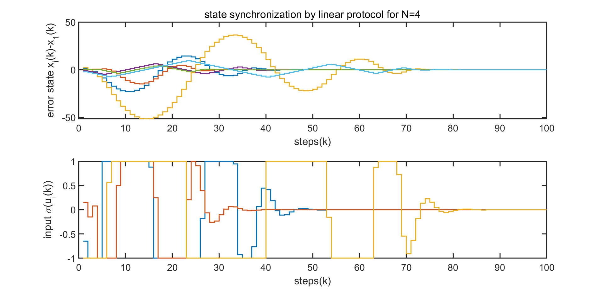
Figure 2: Global state synchronization for MAS with communication graph I when $k_{1}=0.5$ and $k_{2}=1$.

Case II: 7-agent graph

Then, we consider a MAS with $7$ agents $N=7$. The associated adjacency matrix to the communication network is assumed to be $\mathcal{A}_{II}$ where $a_{21}=a_{32}=a_{43}=a_{24}=a_{54}=a_{47}=a_{65}=a_{76}=1$.

In this case, we still use protocol (25). The simulation result are demonstrated in Figure 3.

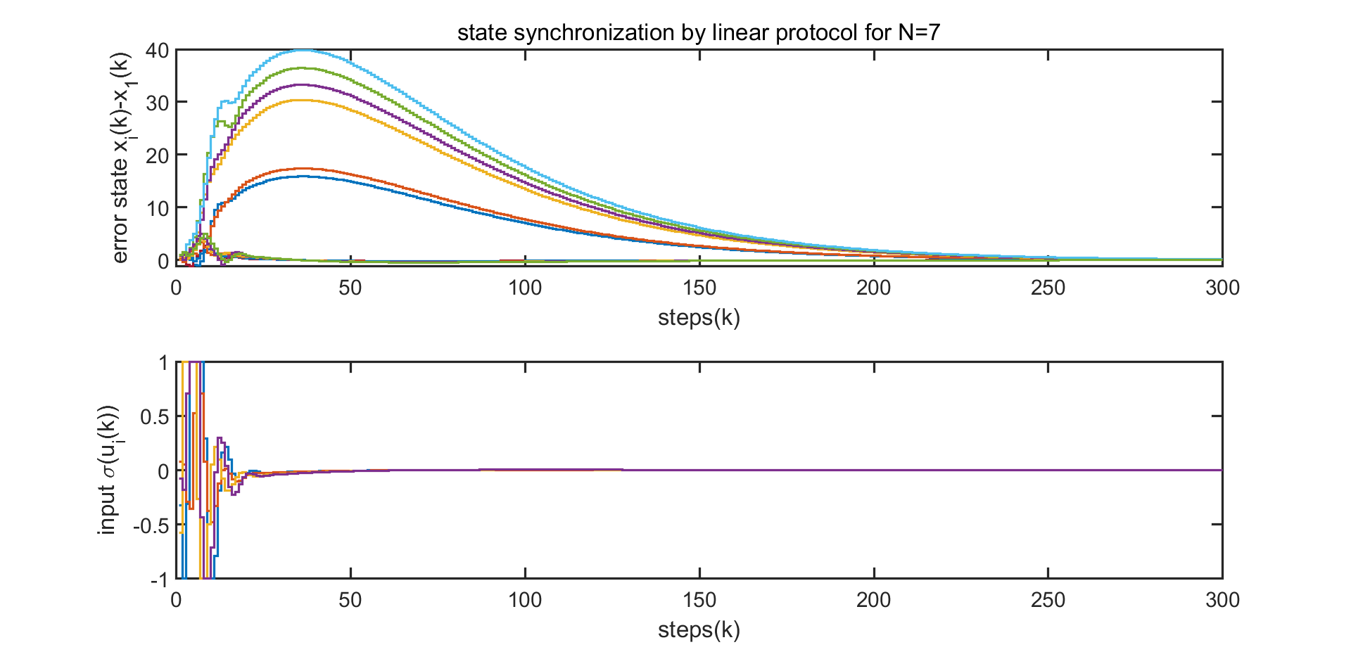
Figure 3: Global state synchronization for MAS with communication graph II when $k_{1}=0.5$ and $k_{2}=1$.

Case III: 60-agent graph

Finally, we consider a MAS with $60$ agents $N=60$ and a directed loop graph, where the associated adjacency matrix is assumed to be $\mathcal{A}_{III}$ only with $a_{i+1,i}=a_{1,60}=1$ and $i=1,\cdots,59$.

The simulation result by using protocol (25) is demonstrated in Figure 4.

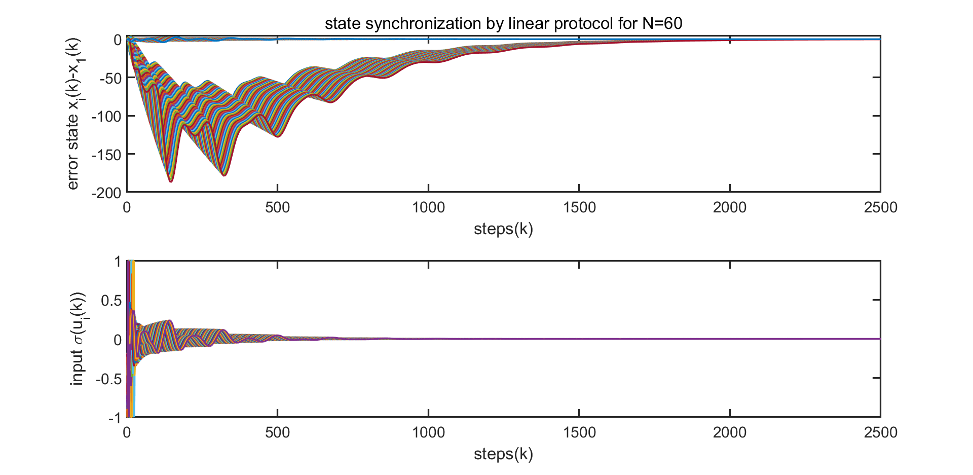
Figure 4: Global state synchronization for MAS with communication graph III when $k_{1}=0.5$ and $k_{2}=1$.

All above simulation results with different graphs show that the protocol design is independent of the communication graph and is scale free so that we can achieve synchronization with one-shot protocol design, for any graph with any number of agents.

5 Conclusion

In this paper, we have developed a scale-free linear protocol design to achieve global state synchronization for discrete-time double-integrator MAS subject to actuator saturation. The scale-free protocols are designed solely based on agent models without utilizing any information and are universal, it means that for any number of agents and any communication graph. Meanwhile, we provide a solvable zone to protocol’s parameter, and all parameter pair in this zone can achieve state synchronization of discrete-time double integrator MAS with input saturation.

References

• [1] H. Bai, M. Arcak, and J. Wen. Cooperative control design: a systematic, passivity-based approach. Communications and Control Engineering. Springer Verlag, 2011.
• [2] F. Bullo. Lectures on network systems. Kindle Direct Publishing, 2019.
• [3] N. Chopra. Output synchronization on strongly connected graphs. IEEE Trans. Aut. Contr., 57(1):2896–2901, 2012.
• [4] D. Chowdhury and H. K. Khalil. Synchronization in networks of identical linear systems with reduced information. In American Control Conference, pages 5706–5711, Milwaukee, WI, 2018.
• [5] H. Chu, J. Yuan, and W. Zhang. Observer-based consensus tracking for linear multi-agent systems with input saturation. IET Control Theory and Applications, 9(14):2124–2131, 2015.
• [6] A. Eichler and H. Werner. Closed-form solution for optimal convergence speed of multi-agent systems with discrete-time double-integrator dynamics for fixed weight ratios. Syst. & Contr. Letters, 71:7–13, 2014.
• [7] C. Godsil and G. Royle. Algebraic graph theory, volume 207 of Graduate Texts in Mathematics. Springer-Verlag, New York, 2001.
• [8] H.F. Grip, T. Yang, A. Saberi, and A.A. Stoorvogel. Output synchronization for heterogeneous networks of non-introspective agents. Automatica, 48(10):2444–2453, 2012.
• [9] C.N. Hadjicostis and T. Charalambous. Average consensus in the presence of delays in directed graph topologies. IEEE Trans. Aut. Contr., 59(3):763–768, 2014.
• [10] H. Kim, H. Shim, J. Back, and J. Seo. Consensus of output-coupled linear multi-agent systems under fast switching network: averaging approach. Automatica, 49(1):267–272, 2013.
• [11] L. Kocarev. Consensus and synchronization in complex networks. Springer, Berlin, 2013.
• [12] T. Li and J. Zhang. Consensus conditions of multi-agent systems with time-varying topologies and stochastic communication noises. IEEE Trans. Aut. Contr., 55(9):2043–2057, 2010.
• [13] Y. Li, J. Xiang, and W. Wei. Consensus problems for linear time-invariant multi-agent systems with saturation constraints. IET Control Theory and Applications, 5(6):823–829, 2011.
• [14] Z. Li, Z. Duan, and G. Chen. Consensus of discrete-time linear multi-agent system with observer-type protocols. Discrete and Continuous Dynamical Systems. Series B, 16(2):489–505, 2011.
• [15] Z. Liu, A. Saberi, and A. A. Stoorvogel. Scale-free collaborative protocols for global regulated state synchronization of discrete-time homogeneous networks of non-introspective agents in presence of input saturation. Int. J. Robust & Nonlinear Control, 2022. Early access, DOI: 10.1002/rnc.6087.
• [16] Z. Liu, A. Saberi, A. A. Stoorvogel, and M. Zhang. Passivity-based state synchronization of homogeneous multiagent systems via static protocol in the presence of input saturation. Int. J. Robust & Nonlinear Control, 28(7):2720–2741, 2018.
• [17] Z. Liu, A. Saberi, A.A. Stoorvogel, and D. Nojavanzadeh. Regulated state synchronization of homogeneous discrete-time multi-agent systems via partial state coupling in presence of unknown communication delays. IEEE Access, 7:7021–7031, 2019.
• [18] Z. Liu, A. Saberi, A.A. Stoorvogel, and D. Nojavanzadeh. Global regulated state synchronization for homogeneous networks of non-introspective agents in presence of input saturation: Scale-free nonlinear and linear protocol designs. Automatica, 119:109041(1–8), 2020.
• [19] Z. Liu, M. Zhang, A. Saberi, and A. A. Stoorvogel. State synchronization of multi-agent systems via static or adaptive nonlinear dynamic protocols. Automatica, 95:316–327, 2018.
• [20] Z. Liu, M. Zhang, A. Saberi, and A.A. Stoorvogel. Passivity based state synchronization of homogeneous discrete-time multi-agent systems via static protocol in the presence of input delay. European Journal of Control, 41:16–24, 2018.
• [21] Z. Meng, Z. Zhao, and Z. Lin. On global leader-following consensus of identical linear dynamic systems subject to actuator saturation. Syst. & Contr. Letters, 62(2):132–142, 2013.
• [22] M. Mesbahi and M. Egerstedt. Graph theoretic methods in multiagent networks. Princeton University Press, Princeton, 2010.
• [23] R. Olfati-Saber and R.M. Murray. Consensus problems in networks of agents with switching topology and time-delays. IEEE Trans. Aut. Contr., 49(9):1520–1533, 2004.
• [24] W. Ren. On consensus algorithms for double-integrator dynamics. IEEE Trans. Aut. Contr., 53(6):1503–1509, 2008.
• [25] W. Ren and R.W. Beard. Consensus seeking in multiagent systems under dynamically changing interaction topologies. IEEE Trans. Aut. Contr., 50(5):655–661, 2005.
• [26] W. Ren and Y.C. Cao. Distributed coordination of multi-agent networks. Communications and Control Engineering. Springer-Verlag, London, 2011.
• [27] A. Saberi, A. A. Stoorvogel, M. Zhang, and P. Sannuti. Synchronization of multi-agent systems in the presence of disturbances and delays. Birkhäuser, Cham, 2022.
• [28] L. Scardovi and R. Sepulchre. Synchronization in networks of identical linear systems. Automatica, 45(11):2557–2562, 2009.
• [29] J.H. Seo, H. Shim, and J. Back. Consensus of high-order linear systems using dynamic output feedback compensator: low gain approach. Automatica, 45(11):2659–2664, 2009.
• [30] H. Su and M.Z.Q. Chen. Multi-agent containment control with input saturation on switching topologies. IET Control Theory and Applications, 9(3):399–409, 2015.
• [31] H. Su, M.Z.Q. Chen, J. Lam, and Z. Lin. Semi-global leader-following consensus of linear multi-agent systems with input saturation via low gain feedback. IEEE Trans. Circ. & Syst.-I Regular papers, 60(7):1881–1889, 2013.
• [32] Y. Su and J. Huang. Stability of a class of linear switching systems with applications to two consensus problem. IEEE Trans. Aut. Contr., 57(6):1420–1430, 2012.
• [33] S.E. Tuna. LQR-based coupling gain for synchronization of linear systems. Available: arXiv:0801.3390v1, 2008.
• [34] S.E. Tuna. Synchronizing linear systems via partial-state coupling. Automatica, 44(8):2179–2184, 2008.
• [35] S.E. Tuna. Conditions for synchronizability in arrays of coupled linear systems. IEEE Trans. Aut. Contr., 55(10):2416–2420, 2009.
• [36] X. Wang, A. Saberi, A.A. Stoorvogel, H.F. Grip, and T. Yang. Synchronization in a network of identical discrete-time agents with uniform constant communication delay. Int. J. Robust & Nonlinear Control, 24(18):3076–3091, 2014.
• [37] P. Wieland, J.S. Kim, and F. Allgöwer. On topology and dynamics of consensus among linear high-order agents. International Journal of Systems Science, 42(10):1831–1842, 2011.
• [38] C.W. Wu. Synchronization in complex networks of nonlinear dynamical systems. World Scientific Publishing Company, Singapore, 2007.
• [39] T. Yang, Z. Meng, D.V. Dimarogonas, and K.H. Johansson. Global consensus for discrete-time multi-agent systems with input saturation constraints. Automatica, 50(2):499–506, 2014.
• [40] K. You and L. Xie. Network topology and communication data rate for consensusability of discrete-time multi-agent systems. IEEE Trans. Aut. Contr., 56(10):2262–2275, 2011.
• [41] L. Zhang, M.Z.Q. Chen, and H. Su. Observer-based semi-global consensus of discrete-time multi-agent systems with input saturation. Transactions of the Institute of Measurement and Control, 38(6):665–674, 2016.
• [42] M. Zhang, A. Saberi, and A.A. Stoorvogel. Synchronization in a network of identical continuous-or discrete-time agents with unknown nonuniform constant input delay. Int. J. Robust & Nonlinear Control, 28(13):3959–3973, 2018.