Existence, uniqueness and approximation of solutions to Carathéodory delay differential equations

Abstract.

In this paper we address the existence, uniqueness and approximation of solutions of delay differential equations (DDEs) with Carathéodory type right-hand side functions. We provide construction of randomized Euler scheme for DDEs and investigate its error. We also report results of numerical experiments.

Mathematics Subject Classification: 65C20, 65C05, 65L05

1. Introduction

We deal with approximation of solutions to the following delay differential equations (DDEs)

(1.1) $$\begin{cases}x^{\prime}(t)=f(t,x(t),x(t-\tau)),&t\in[0,(n+1)\tau],\\ x(t)=x_{0},&t\in[-\tau,0),\end{cases}$$

with the constant time-lag $\tau\in(0,+\infty)$, fixed time horizon $n\in\mathbb{N}$, $f:[0,(n+1)\tau]\times\mathbb{R}^{d}\times\mathbb{R}^{d}\mapsto\mathbb{R}^{d}$, and $x_{0}\in\mathbb{R}^{d}$. We assume that $f$ is integrable with respect to $t$ and (at least) continuous with respect to $(x,z)$. Hence, we consider Carathéodory type conditions for $f$.

Motivation of considering such DDEs comes, for example, from the problem of modeling switching systems with memory, see [7], [8]. Moreover, another inspiration follows from delayed differential equations with rough paths of the form

(1.2) $$\begin{cases}\mathrm{d}U(t)=a(U(t),U(t-\tau))+\mathrm{d}Z(t),&t\in[0,(n+1)\tau],\\ U(t)=U_{0},&t\in[-\tau,0),\end{cases}$$

where $Z$ is an integrable perturbation (which might be of stochastic nature). Then $x(t)=U(t)-Z(t)$ satisfies the (possibly random) DDE (1.1) with $f(t,x,z)=a(x+Z(t),z+Z(t-\tau))$ and $x(t)=U_{0}$, where we assume that $Z(t)=0$ for $t\in[-\tau,0]$. In this case the function $f$ inherits from $Z$ its low smoothness with respect to the variable $t$. (The exemplary equation (1.2) is a generalization of the ODE with rough paths discussed in [14].)

In the case of classical assumptions (such as $C^{r}$-regularity of $f=f(t,x,z)$ wrt all variables $t,x,z$) imposed on the right-hand side function errors for deterministic schemes have been established, for example, in the book [2], which is the standard reference. See also [5], where error of the Euler scheme has been investigated for some class of nonlinear DDEs under nonstandard assumptions, such as one-side Lipschitz condition and local Hölder continuity. In contrast, much less is known about the approximation of solutions of DDEs with less regular Carathéodory right-hand side function $f$. In the case of Carathéodory ODEs we need to turn to randomized algorithms, such as randomized Euler scheme, since it is well-known that there is lack of convergence for deterministic algorithms, see [14]. This behavior is inherited by DDEs, since ODEs form a subclass of DDEs. Hence, we define randomized version of the Euler scheme that is suitable for DDEs of the form (1.1).

While the randomized algorithms for ODEs have been widely investigated in the literature (see, for example, [4], [3], [6], [9], [10], [11], [14]), according to our best knowledge this is the first paper that defines randomized Euler scheme and rigorously investigates its error for (Carathéodory type) DDEs.

The main contributions of the paper are as follows:

• we show existence, uniqueness, and Hölder regularity of the solution to (1.1) when the right-hand side function $f=f(t,x,z)$ is only integrable with respect to $t$ and satisfies local Lipschitz assumption with respect to $(x,z)$ (Theorem 3.1),

• we perform rigorous error analysis of the randomized Euler scheme applied to (1.1) when the right-hand side function $f=f(t,x,z)$ is only integrable with respect to $t$, satisfies global Lipschitz condition with respect to $x$ and it is globally Hölder continuous with respect to $z$ (Theorem 4.2),

• we report results of numerical experiments that show stable error behaviour as stated in Theorem 4.2.

In addition, as a consequence of Theorem 3.1 we establish almost sure convergence of the randomized Euler scheme, see Proposition 4.3.

We want to stress here that the techniques used when proving upper error bounds in Theorem 4.2 differ significantly comparing to that used in [4], [3], [6], [9], [10], [14] for randomized algorithms defined for ordinary differential equations. Mainly, due to the fact that DDEs have to be considered interval-by-interval we developed a suitable proof technique that is based on mathematical induction. In particular, suitable inductive assumptions have to be related with the Hölder continuity of $f=f(t,x,z)$ with respect to the (delayed) variable $z$. It can be observed from the proof that the main result from [14] can be applied only for the initial inductive step, when the Hölder continuity of $f$ with respect to $z$ does not make an impact, equivalently, when the CDDE and its numerical counter part are subject to the same value of the delay variable. As the systems iterate over time, a different strategy is required to handle the effect of the delay variable. An auxiliary randomized Euler scheme, which is not practical but theoretically useful, is therefore introduced for error decomposition to leverage the inductive estimate from previous steps as well as the randomized quadrature rule from [14].

The structure of the article is as follows. Basic notions, definitions together with assumptions and definition of the randomized Euler scheme are given in Section 2. All Section 3 is devoted to the issue of existence and uniqueness of solutions of the Carathéodory type DDEs (1.1) in the case when $f=f(t,x,z)$ is only integrable with respect to $t$ and satisfies local Lipschitz assumption with respect to $(x,z)$. Section 4 contain proof of the main result of the paper (Theorem 3.1) that states upper bounds on the error of the randomized Euler scheme. In Section 5 we report results of numerical experiments. Finally, Appendix contains auiliary results for Carathéodory type ODEs that we use in the paper.

2. Preliminaries

By $\|\cdot\|$ we mean the Euclidean norm in $\mathbb{R}^{d}$. We consider a complete probability space $(\Omega,\Sigma,\mathbb{P})$. For a random variable $X:\Omega\to\mathbb{R}$ we denote by $\|X\|_{L^{p}(\Omega)}=(\mathbb{E}|X|^{p})^{1/p}$, where $p\in[2,+\infty)$.

Let us fix the horizon parameter $n\in\mathbb{N}$. On the right-hand side function $f$ we impose the following assumptions:

1. $f(t,\cdot,\cdot)\in C(\mathbb{R}^{d}\times\mathbb{R}^{d};\mathbb{R}^{d})$ for all $t\in[0,(n+1)\tau]$,

2. $f(\cdot,x,z)$ is Borel measurable for all $(x,z)\in\mathbb{R}^{d}\times\mathbb{R}^{d}$,

3. there exists $K:[0,(n+1)\tau]\to[0,+\infty)$ such that $K\in L^{1}([0,(n+1)\tau])$ and for all $(t,x,z)\in[0,(n+1)\tau]\times\mathbb{R}^{d}\times\mathbb{R}^{d}$

   (2.1) $$\|f(t,x,z)\|\leq K(t)(1+\|x\|)(1+\|z\|),$$

4. for every compact set $U\subset\mathbb{R}^{d}$ there exists $L_{U}:[0,(n+1)\tau]\mapsto[0,+\infty)$ such that $L_{U}\in L^{1}([0,(n+1)\tau])$ and for all $t\in[0,(n+1)\tau]$, $x_{1},x_{2}\in U$, $z\in\mathbb{R}^{d}$

   (2.2) $$\|f(t,x_{1},z)-f(t,x_{2},z)\|\leq L_{U}(t)(1+\|z\|)\|x_{1}-x_{2}\|.$$

In Section 3, under the assumptions (A1)-(A4), we investigate existence and uniqueness of solution for (1.1). Next, in Section 4 we investigate error of the randomized Euler scheme under slightly stronger assumptions. Namely, we impose global Lipschitz assumption on $f=(t,x,z)$ with respect to $(x,z)$ instead of its local version (A4).

The mentioned above randomized Euler scheme is defined as follows. Fix the discretization parameter $N\in\mathbb{N}$ and set

$$t_{k}^{j}=j\tau+kh,\quad k=0,1,\ldots,N,\ j=0,1,\ldots,n,$$

where

(2.3) $$h=\frac{\tau}{N}.$$

Note that for each $j$ the sequence $\{t^{j}_{k}\}_{k=0}^{N}$ provides uniform discretization of the subinterval $[j\tau,(j+1)\tau]$. Let $\{\gamma_{k}^{j}\}_{j\in\mathbb{N}_{0},k\in\mathbb{N}}$ be an iid sequence of random variables, defined on the complete probability space $(\Omega,\Sigma,\mathbb{P})$, where every $\gamma_{k}^{j}$ is uniformly distributed on $[0,1]$. We set $y_{0}^{-1}=\ldots=y^{-1}_{N}=x_{0}$ and then for $j=0,1,\ldots,n$, $k=0,1,\ldots,N-1$ we take

(2.4) $$y_{0}^{j}=y^{j-1}_{N},$$

(2.5) $$y_{k+1}^{j}=y_{k}^{j}+h\cdot f(\theta_{k+1}^{j},y_{k}^{j},y_{k}^{j-1}),$$

where $\theta_{k+1}^{j}=t_{k}^{j}+h\gamma_{k+1}^{j}$. As the output we obtain the sequence of $\mathbb{R}^{d}$-valued random vectors $\{y_{k}^{j}\}_{k=0,1,\ldots,N},j=0,1,\ldots,n$ that provides a discrete approximation of the values $\{x(t_{k}^{j})\}_{k=0,1,\ldots,N},j=0,1,\ldots,n$. It is easy to see that each random vector $y_{k}^{j}$, $j=0,1,\ldots,n$, $k=0,1,\ldots,N$, is measurable with respect to the $\sigma$-field generated by the following family of independent random variables

(2.6) $$\Bigl{\{}\theta_{1}^{0}\ldots,\theta_{N}^{0},\ldots,\theta_{1}^{j-1},\ldots,\theta_{N}^{j-1},\theta_{1}^{j},\ldots,\theta_{k}^{j}\Bigr{\}}.$$

As the horizon parameter $n$ is fixed, the randomized Euler scheme uses $O(N)$ evaluations of $f$ (with a constant in the ’$O$’ notation that only depends on $n$ but not on $N$).

In Section 4 we provide upper bounds on the error

(2.7) $$\Bigl{\|}\max\limits_{0\leq i\leq N}\|x(t_{i}^{j})-y_{i}^{j}\|\Bigl{\|}_{L^{p}(\Omega)}$$

for $j=0,1,\ldots,n$.

3. Properties of solutions to Carathéodory DDEs

In this section we investigate the issue of existence and uniqueness of the solution of (1.1) under the assumptions (A1)-(A4).

In the sequel we use the following equivalent representation of the solution of (1.1), that is very convenient when proving its properties and when estimating the error of the randomized Euler scheme. For $j=0,1,\ldots,n$ and $t\in[0,\tau]$ it holds

(3.1) $$x^{\prime}(t+j\tau)=f(t+j\tau,x(t+j\tau),x(t+(j-1)\tau)).$$

Hence, we take $\phi_{-1}(t):=x_{0}$, $\phi_{j}(t)\mathrel{\mathop{:}}=x(t+j\tau)$ and for $j=0,1,\ldots,n$ we consider the following sequence of initial-value problems

(3.2) $$\begin{cases}\phi_{j}^{\prime}(t)=g_{j}(t,\phi_{j}(t)),&t\in[0,\tau],\\ \phi_{j}(0)=\phi_{j-1}(\tau),\end{cases}$$

with $g_{j}(t,x)=f(t+j\tau,x,\phi_{j-1}(t))$, $(t,x)\in[0,\tau]\times\mathbb{R}^{d}$. Then the solution of (1.1) can be written as

(3.3) $$x(t)=\sum\limits_{j=-1}^{n}\phi_{j}(t-j\tau)\cdot\mathbf{1}_{[j\tau,(j+1)\tau]}(t),\quad t\in[-\tau,(n+1)\tau].$$

We prove the following result about existence, uniqueness and Hölder regularity of the solution of the delay differential equation (1.1). We will use this theorem in the next section when proving error estimate for the randomized Euler algorithm.

Theorem 3.1.

Let $n\in\mathbb{N}\cup\{0\}$, $\tau\in(0,+\infty)$, $x_{0}\in\mathbb{R}^{d}$ and let $f$ satisfy assumptions (A1)-(A4). Then there exists a unique absolutely continuous solution $x=x(x_{0},f)$ to (1.1) such that for $j=0,1,\ldots,n$ we have

$$\sup\limits_{0\leq t\leq\tau}\|\phi_{j}(t)\|\leq K_{j}$$

where $K_{-1}:=\|x_{0}\|$ and

(3.4) $$K_{j}=(1+K_{j-1})(1+\|K\|_{L^{1}([j\tau,(j+1)\tau])})\cdot\exp\Bigl{(}(1+K_{j-1})\|K\|_{L^{1}([j\tau,(j+1)\tau])}\Bigr{)}.$$

Moreover, if we additionally assume that for some $p\in(1,+\infty]$ the function $K$ in (A3) satisfies

1. $K\in L^{p}([0,(n+1)\tau])$,

then for all $j=0,1,\ldots,n$, $t,s\in[0,\tau]$ it holds

(3.5) $$\|\phi_{j}(t)-\phi_{j}(s)\|\leq(1+K_{j-1})(1+K_{j})\|K\|_{L^{p}([j\tau,(j+1)\tau])}|t-s|^{1-\frac{1}{p}}.$$

Proof.

We proceed by induction. We start with the case when $j=0$ and consider the following initial-value problem

(3.6) $$\begin{cases}\phi_{0}^{\prime}(t)=g_{0}(t,\phi_{0}(t)),&t\in[0,\tau],\\ \phi_{0}(0)=x_{0},\end{cases}$$

with $g_{0}(t,x)=f(t,x,\phi_{-1}(t))=f(t,x,x_{0})$. Of course for all $t\in[0,\tau]$ the function $g_{0}(t,\cdot)$ is continuous and for all $x\in\mathbb{R}^{d}$ the function $g_{0}(\cdot,x)$ is Borel measurable. Moreover, by (2.1) we have $\|g_{0}(t,x)\|\leq K(t)(1+\|x_{0}\|)(1+\|x\|)$ for all $(t,x)\in[a,b]\times\mathbb{R}^{d}$, and by (2.2) for every compact set $U$ in $\mathbb{R}^{d}$ there exists a positive function $L_{U}\in L^{1}([0,(n+1)\tau])$ such that for all $t\in[0,\tau]$, $x,y\in U$ it holds

(3.7) $$\|g_{0}(t,x)-g_{0}(t,y)\|\leq L_{U}(t)(1+\|x_{0}\|)\|x-y\|.$$

Therefore, by Lemma 7.1 we have that there exists a unique absolutely continuous solution $\phi_{0}:[0,\tau]\to\mathbb{R}^{d}$ of (3.6) that satisfies (3.1) with $j=0$. In addition, if $K\in L^{p}([0,(n+1)\tau])$ for some $p\in(1,+\infty]$ then by Lemma 7.1 we obtain that $\phi_{0}$ satisfies (3.5) for $j=0$.

Let us now assume that for some $j\in\{0,1,\ldots,n-1\}$ there exists a unique absolutely continuous solution $\phi_{j}:[0,\tau]\to\mathbb{R}^{d}$ of

(3.8) $$\begin{cases}\phi_{j}^{\prime}(t)=g_{j}(t,\phi_{j}(t)),&t\in[0,\tau],\\ \phi_{j}(0)=\phi_{j-1}(\tau),\end{cases}$$

where $g_{j}(t,x)=f(t+j\tau,x,\phi_{j-1}(t))$, and that satisfies (3.1) with (3.5), if $K\in L^{p}([0,(n+1)\tau])$ for some $p\in(1,+\infty]$. We consider the following initial-value problem

(3.9) $$\begin{cases}\phi_{j+1}^{\prime}(t)=g_{j+1}(t,\phi_{j+1}(t)),&t\in[0,\tau],\\ \phi_{j+1}(0)=\phi_{j}({\tau}),\end{cases}$$

with $g_{j+1}(t,x)=f(t+(j+1)\tau,x,\phi_{j}(t))$. Since $\phi_{j}$ is continuous on $[0,\tau]$, it is straightforward to see that for all $t\in[0,\tau]$ the function $g_{j+1}(t,\cdot)$ is continuous and for all $x\in\mathbb{R}^{d}$ the function $g_{j+1}(\cdot,x)$ is Borel measurable. Moreover, by (3.1) for all $(t,x)\in[0,\tau]\times\mathbb{R}^{d}$

$$\|g_{j+1}(t,x)\|\leq K(t+(j+1)\tau)(1+\|\phi_{j}(t)\|)(1+\|x\|)$$

(3.10) $$\leq K(t+(j+1)\tau)(1+K_{j})(1+\|x\|),$$

where

(3.11) $$\int\limits_{0}^{\tau}K(t+(j+1)\tau)\,\mathrm{d}t=\int\limits_{(j+1)\tau}^{(j+2)\tau}K(t)\,\mathrm{d}t\leq\int\limits_{0}^{(n+1)\tau}K(t)\,\mathrm{d}t<+\infty.$$

Furthermore, by (2.2) and (3.1) for every compact set $U$ in $\mathbb{R}^{d}$ there exists a positive function $L_{U}\in L^{1}([0,(n+1)\tau])$ such that for all $t\in[0,\tau]$, $x,y\in U$ it holds

(3.12) $$\|g_{j+1}(t,x)-g_{j+1}(t,y)\|\leq L_{U}(t+(j+1)\tau)(1+K_{j})\|x-y\|,$$

where

(3.13) $$\int\limits_{0}^{\tau}L_{U}(t+(j+1)\tau)\,\mathrm{d}t=\int\limits_{(j+1)\tau}^{(j+2)\tau}L_{U}(t)\,\mathrm{d}t\leq\int\limits_{0}^{(n+1)\tau}L_{U}(t)\,\mathrm{d}t<+\infty.$$

Hence, by Lemma 7.1 there exists a unique absolutely continuous solution $\phi_{j+1}:[0,\tau]\to\mathbb{R}^{d}$ of (3.9). By the inductive assumption and Lemma 7.1 we get that

$$\sup\limits_{0\leq t\leq\tau}\|\phi_{j+1}(t)\|\leq\Bigl{(}\|\phi_{j}(\tau)\|+(1+K_{j})\int\limits_{0}^{\tau}K(t+(j+1)\tau)\,\mathrm{d}t\Bigr{)}$$

$$\times\exp\Bigl{(}(1+K_{j})\int\limits_{0}^{\tau}K(t+(j+1)\tau)\,\mathrm{d}t\Bigr{)}$$

$$\leq(1+K_{j})(1+\|K\|_{L^{1}([(j+1)\tau,(j+2)\tau])})\exp\Bigl{(}(1+K_{j})\|K\|_{L^{1}([(j+1)\tau,(j+2)\tau])}\Bigr{)}=K_{j+1},$$

and

(3.14) $$\|\phi_{j+1}(t)-\phi_{j+1}(s)\|\leq\bar{K}_{j+1}|t-s|^{1-\frac{1}{p}},$$

where

$$\bar{K}_{j+1}=(1+K_{j})\Bigl{(}\int\limits_{0}^{\tau}|K(t+(j+1)\tau)|^{p}\,\mathrm{d}t\Bigr{)}^{1/p}$$

$$\times\Biggl{(}1+\Bigl{(}\|\phi_{j}(\tau)\|+(1+K_{j})\int\limits_{0}^{\tau}K(t+(j+1)\tau)\,\mathrm{d}t\Bigr{)}\exp\Bigl{(}(1+K_{j})\int\limits_{0}^{\tau}K(t+(j+1)\tau)\,\mathrm{d}t\Bigr{)}\Biggr{)}$$

$$\leq(1+K_{j})\|K\|_{L^{p}([(j+1)\tau,(j+2)\tau])}(1+K_{j+1}).$$

This ends the inductive proof. ∎

Remark 3.2.

Theorem 3.1 can be applied, for example, to the function

(3.15) $$f(t,x,z)=K(t)\cdot\cos(x^{2})\cdot|z|^{\alpha},\quad(t,x,z)\in[0,(n+1)\tau]\times\mathbb{R}\times\mathbb{R},$$

where $K$ is any function from $L^{1}([0,(n+1)\tau])$ and $\alpha\in(0,1]$.

4. Error of the randomized Euler scheme

In this section we perform detailed error analysis for the randomized Euler. As mentioned in Section 1, for the error analysis we impose global Lipschitz assumption on $f=f(t,x,z)$ with respect to $x$ together with global Hölder condition with respect to $z$. Namely, instead of (A3) and (A4), we assume

1. there exist $p\in[2,+\infty]$, $\alpha\in(0,1]$ and $\bar{K},L:[0,(n+1)\tau]\to[0,+\infty)$ such that $\bar{K},L\in L^{p}([0,(n+1)\tau])$ and for all $t\in[0,(n+1)\tau]$

   (4.1) $$\|f(t,0,0)\|\leq\bar{K}(t),$$

   and for all $t\in[0,(n+1)\tau]$, $x_{1},x_{2},z_{1},z_{2}\in\mathbb{R}^{d}$

   (4.2) $$\|f(t,x_{1},z_{1})-f(t,x_{2},z_{2})\|\leq L(t)\Bigl{(}\|x_{1}-x_{2}\|+\|z_{1}-z_{2}\|^{\alpha}\Bigr{)}.$$

Remark 4.1.

Note that the assumptions (A1), (A2), (A3’) are stronger than the assumptions (A1)-(A4). To see that note that if $f$ satisfies (A1), (A2), (A3’) then we get for all $t\in[0,(n+1)\tau]$ and $x,x_{1},x_{2},z\in\mathbb{R}^{d}$ that

(4.3) $$\|f(t,x,z)\|\leq(\bar{K}(t)+L(t))(1+\|x\|)(1+\|z\|),$$

and

(4.4) $$\|f(t,x_{1},z)-f(t,x_{2},z)\|\leq L(t)\|x_{1}-x_{2}\|,$$

since $1+\|x\|+\|z\|\leq(1+\|x\|)(1+\|z\|)$ and $\|z\|^{\alpha}\leq 1+\|z\|$ for all $x,z\in\mathbb{R}^{d}$. Hence, the assumptions (A1)-(A4) are satisfied with $K=\bar{K}+L\in L^{p}([0,(n+1)\tau])$, $L_{U}=L\in L^{p}([0,(n+1)\tau])$ for any compact set $U\subset\mathbb{R}^{d}$, and under the assumptions (A1), (A2), (A3’) the thesis of Theorem 3.1 holds.

The main result of this section is as follows.

Theorem 4.2.

Let $n\in\mathbb{N}\cup\{0\}$, $\tau\in(0,+\infty)$, $x_{0}\in\mathbb{R}^{d}$, and let $f$ satisfy the assumptions (A1), (A2), (A3’) for some $p\in[2,+\infty)$ and $\alpha\in(0,1]$. There exist $C_{0},C_{1},\ldots,C_{n}\in(0,+\infty)$ such that for all $N\geq\lceil\tau\rceil$ and $j=0,1,\ldots,n$ it holds

(4.5) $$\Bigl{\|}\max\limits_{0\leq i\leq N}\|x(t_{i}^{j})-y_{i}^{j}\|\Bigl{\|}_{L^{p}(\Omega)}\leq C_{j}h^{\frac{1}{2}\alpha^{j}}.$$

In particular, if $\alpha=1$ then for $j=0,1,\ldots,n$

(4.6) $$\Bigl{\|}\max\limits_{0\leq i\leq N}\|x(t_{i}^{j})-y_{i}^{j}\|\Bigl{\|}_{L^{p}(\Omega)}\leq C_{j}h^{1/2}.$$

Proof.

In the proof we use the following auxiliary notation: $\alpha_{k}^{j}=k+\gamma_{k+1}^{j}$ and $\delta_{k+1}^{j}=h\cdot\alpha_{k}^{j}$. Then $\delta_{k+1}^{j}$ is uniformly distributed in $(t_{k}^{0},t_{k+1}^{0})$ and $\theta_{k+1}^{j}=\delta_{k+1}^{j}+j\tau$ is uniformly distributed in $(t_{k}^{j},t_{k+1}^{j})$.

We start with $j=0$ and consider the initial-vale problem (3.6). We define the auxiliary randomized Euler scheme as

(4.7) $$\bar{y}_{0}^{0}=y^{0}_{0}=y^{-1}_{N}=x_{0},$$

(4.8) $$\bar{y}_{k+1}^{0}=\bar{y}_{k}^{0}+h\cdot g_{0}(\theta_{k+1}^{0},\bar{y}_{k}^{0}),\ k=0,1,\ldots,N-1.$$

Since $\bar{y}_{0}^{0}=y_{0}^{0}=x_{0}$ and $g_{0}(t,x)=f(t,x,x_{0})$, for all $k=0,\ldots,N$ we have that $\bar{y}_{k}^{0}=y_{k}^{0}$. Moreover, by (A1), (A2) and (A3’) we have that $g_{0}$ is Borel measurable, and for all $t\in[0,\tau]$ and $x,y\in\mathbb{R}^{d}$

$$\|g_{0}(t,x)\|\leq K(t)(1+\|x_{0}\|)(1+\|x\|),$$

(4.9) $$\|g_{0}(t,x)-g_{0}(t,y)\|\leq L(t)\|x-y\|,$$

where $K=\bar{K}+L$, as stated in Remark 4.1. Hence, by Theorem 3.1 and by using analogous arguments as in the proof of Theorem 4.3 in [14] we get

$$\Bigl{\|}\max\limits_{0\leq i\leq N}\|\phi_{0}(t_{i}^{0})-y_{i}^{0}\|\Bigl{\|}_{L^{p}(\Omega)}\leq 2^{1-\frac{1}{p}}\exp\Bigl{(}\frac{(2\tau)^{p-1}}{p}\|L\|^{p}_{L^{p}([0,\tau])}\Bigr{)}$$

$$\times(1+K_{-1})(1+K_{0})\|K\|_{L^{p}([0,\tau])}\Bigl{(}2C_{p}\tau^{\frac{p-2}{2p}}+\tau^{1-\frac{1}{p}}\|L\|_{L^{p}([0,\tau])}\Bigr{)}h^{1/2}=C_{0}h^{1/2},$$

where $C_{0}$ does not depend on $N$. Since $\phi_{0}(t_{i}^{0})=x(t_{i}^{0})$ we get (4.5) for $j=0$.

Let us now assume that there exists $l\in\{0,1,\ldots,n-1\}$ for which there exists $C_{l}\in(0,+\infty)$ such that for all $N\geq\lceil\tau\rceil$

(4.10) $$\Bigl{\|}\max\limits_{0\leq i\leq N}\|\phi_{l}(t_{i}^{0})-y_{i}^{l}\|\Bigl{\|}_{L^{p}(\Omega)}\leq C_{l}h^{\frac{1}{2}\alpha^{l}}.$$

We consider the following initial-value problem

(4.11) $$\begin{cases}\phi_{l+1}^{\prime}(t)=g_{l+1}(t,\phi_{l+1}(t)),&t\in[0,\tau],\\ \phi_{l+1}(0)=\phi_{l}({\tau}),\end{cases}$$

with $g_{l+1}(t,x)=f(t+(l+1)\tau,x,\phi_{l}(t))$. Recall that by (A1), (A2), (A3’), Theorem 3.1, and Remark 4.1 the function $g_{l+1}$ is Borel measurable and for all $t\in[0,\tau]$, $x,y\in\mathbb{R}^{d}$ it satisfies

(4.12) $$\|g_{l+1}(t,x)\|\leq K(t+(l+1)\tau)(1+K_{l})(1+\|x\|),$$

(4.13) $$\|g_{l+1}(t,x)-g_{l+1}(t,y)\|\leq L(t+(l+1)\tau)\|x-y\|.$$

We define the auxiliary randomized Euler scheme as follows

(4.14) $$\bar{y}_{0}^{l+1}=y^{l+1}_{0}=y^{l}_{N},$$

(4.15) $$\bar{y}_{k+1}^{l+1}=\bar{y}_{k}^{l+1}+h\cdot g_{l+1}(\alpha_{k}^{l+1}\cdot h,\bar{y}_{k}^{l+1}),\ k=0,1,\ldots,N-1.$$

From the definition it follows that $\bar{y}_{k}^{j}$, $j=0,1,\ldots,n$, $k=0,1,\ldots,N$, is measurable with respect to the $\sigma$-filed generated by (2.6), so as $y_{k}^{j}$. Moreover, $\bar{y}^{l+1}_{i}$ approximates $\phi_{l+1}$ at $t_{i}^{0}$, however $\{\bar{y}_{i}^{l+1}\}_{i=0,1,\ldots,N}$ is not implementable. We use $\bar{y}^{l+1}_{i}$ only in order to estimate the error (4.5) of $y^{l+1}_{i}$, since it holds

(4.16) $$\Bigl{\|}\max\limits_{0\leq i\leq N}\|\phi_{l+1}(t_{i}^{0})-y_{i}^{l+1}\|\Bigl{\|}_{L^{p}(\Omega)} \leq\Bigl{\|}\max\limits_{0\leq i\leq N}\|\phi_{l+1}(t_{i}^{0})-\bar{y}_{i}^{l+1}\|\Bigl{\|}_{L^{p}(\Omega)}$$

$$\quad+\Bigl{\|}\max\limits_{0\leq i\leq N}\|\bar{y}_{i}^{l+1}-y_{i}^{l+1}\|\Bigl{\|}_{L^{p}(\Omega)}.$$

Firstly, we estimate $\displaystyle{\Bigl{\|}\max\limits_{0\leq i\leq N}\|\bar{y}_{i}^{l+1}-y_{i}^{l+1}\|\Bigl{\|}_{L^{p}(\Omega)}}$. For $k\in\{1,\ldots,N\}$ we get

$$\bar{y}^{l+1}_{k}-y^{l+1}_{k} =\sum\limits_{j=1}^{k}(\bar{y}^{l+1}_{j}-\bar{y}^{l+1}_{j-1})-\sum\limits_{j=1}^{k}(y^{l+1}_{j}-y^{l+1}_{j-1})$$

$$=h\sum\limits_{j=1}^{k}\Bigl{(}f(\theta_{j}^{l+1},\bar{y}^{l+1}_{j-1},\phi_{l}(\alpha_{j-1}^{l+1}\cdot h))-f(\theta_{j}^{l+1},y^{l+1}_{j-1},y^{l}_{j-1})\Bigr{)},$$

which gives

$$\|\bar{y}^{l+1}_{k}-y^{l+1}_{k}\|\leq h\sum\limits_{j=1}^{k}L(\theta_{j}^{l+1})\cdot\|\bar{y}^{l+1}_{j-1}-y^{l+1}_{j-1}\|+h\sum\limits_{j=1}^{k}L(\theta_{j}^{l+1})\cdot\|\phi_{l}(\alpha_{j-1}^{l+1}\cdot h)-y^{l}_{j-1}\|^{\alpha}.$$

Note that the random variables $L(\theta_{j}^{l+1})$ and $\|\phi_{l}(\alpha_{j-1}^{l+1}\cdot h)-y^{l}_{j-1}\|^{\alpha}$ are not independent. However, by Theorem 3.1 we get

$$\|\phi_{l}(\alpha_{j-1}^{l+1}\cdot h)-y^{l}_{j-1}\| \leq\|\phi_{l}(\alpha_{j-1}^{l+1}\cdot h)-\phi_{l}(t_{j-1}^{0})\|+\|\phi_{l}(t_{j-1}^{0})-y^{l}_{j-1}\|$$

$$\leq(1+K_{l-1})(1+K_{l})\|K\|_{L^{p}([l\tau,(l+1)\tau])}\cdot h^{1-\frac{1}{p}}+\|\phi_{l}(t_{j-1}^{0})-y_{j-1}^{l}\|.$$

Therefore for $k\in\{1,\ldots,N\}$

$$\|\bar{y}^{l+1}_{k}-y^{l+1}_{k}\| \leq h\sum\limits_{j=1}^{k}L(\theta_{j}^{l+1})\cdot\max\limits_{0\leq i\leq j-1}\|\bar{y}^{l+1}_{i}-y^{l+1}_{i}\|$$

$$\quad+h\Bigl{(}\sum\limits_{j=1}^{k}L(\theta_{j}^{l+1})\Bigr{)}\cdot\Bigl{(}c_{l+1}h^{\alpha(1-\frac{1}{p})}+\max\limits_{0\leq i\leq N}\|\phi_{l}(t_{i}^{0})-y_{i}^{l}\|^{\alpha}\Bigr{)}.$$

Since $\|\bar{y}^{l+1}_{0}-y^{l+1}_{0}\|=0$ and due to the fact that the random variables $\Bigl{(}\sum\limits_{j=1}^{k}L(\theta_{j}^{l+1})\Bigr{)}$, $\max\limits_{0\leq i\leq N}\|\phi_{l}(t_{i}^{0})-y^{l}_{i}\|^{\alpha}$ are independent, we get

$$\begin{split}\mathbb{E}\Bigl{(}\max\limits_{0\leq i\leq k}\|\bar{y}^{l+1}_{i}-y^{l+1}_{i}\|^{p}\Bigr{)}\leq c_{p}h^{p}\mathbb{E}\Bigl{[}\sum\limits_{j=1}^{k}L(\theta_{j}^{l+1})\cdot\max\limits_{0\leq i\leq j-1}\|\bar{y}^{l+1}_{i}-y^{l+1}_{i}\|\Bigr{]}^{p}\\ +\tilde{c}_{p}\mathbb{E}\Bigl{[}h\sum\limits_{j=1}^{k}L(\theta_{j}^{l+1})\Bigr{]}^{p}\cdot\Bigl{(}\tilde{c}_{l+1}h^{\alpha(p-1)}+\mathbb{E}\Bigl{[}\max\limits_{0\leq i\leq N}\|\phi_{l}(t_{i}^{0})-y_{i}^{l}\|^{\alpha p}\Bigr{]}\Bigr{)}.\end{split}$$

By Jensen inequality and (4.10) we have

(4.17) $$\mathbb{E}\Bigl{[}\max\limits_{0\leq i\leq N}\|\phi_{l}(t_{i}^{0})-y_{i}^{l}\|^{\alpha p}\Bigr{]}\leq\Biggl{(}\mathbb{E}\Bigl{[}\max\limits_{0\leq i\leq N}\|\phi_{l}(t_{i}^{0})-y_{i}^{l}\|^{p}\Bigr{]}\Biggr{)}^{\alpha}\leq C_{l}^{p}h^{\frac{p}{2}\alpha^{l}}.$$

Since the random variables $L(\theta_{j}^{l+1})$ and $\max\limits_{0\leq i\leq j-1}\|\bar{y}_{i}^{l+1}-y_{i}^{l+1}\|$ are independent, $\theta_{j}^{l+1}\sim U(t_{j-1}^{l+1},t_{j}^{l+1})$, we get by the Hölder inequality

(4.18) $$h^{p}\mathbb{E}\Bigl{[}\sum\limits_{j=1}^{k}L(\theta_{j}^{l+1})\cdot\max\limits_{0\leq i\leq j-1}\|\bar{y}^{l+1}_{i}-y^{l+1}_{i}\|\Bigr{]}^{p}\leq\tau^{p-1}\sum\limits_{j=1}^{k}\int\limits_{t_{j-1}^{l+1}}^{t_{j}^{l+1}}(L(t))^{p}\mathrm{d}t\cdot\mathbb{E}\Bigl{[}\max\limits_{0\leq i\leq j-1}\|\bar{y}_{i}^{l+1}-y_{i}^{l+1}\|^{p}\Bigr{]},$$

and

(4.19) $$h^{p}\cdot\mathbb{E}\Bigl{(}\sum\limits_{j=1}^{k}L(\theta_{j}^{l+1})\Bigr{)}^{p}\leq\tau^{p-1}\int\limits_{(l+1)\tau}^{(l+2)\tau}(L(t))^{p}\,\mathrm{d}t<+\infty.$$

Combining (4.17), (4.18), (4.19), and using again the fact that $\bar{y}_{0}^{l+1}=y_{0}^{l+1}$ we arrive at

$$\mathbb{E}\Bigl{(}\max\limits_{0\leq i\leq k}\|\bar{y}^{l+1}_{i}-y^{l+1}_{i}\|^{p}\Bigr{)}\leq\bar{C}_{2,l+1}h^{\frac{p}{2}\alpha^{l+1}}+\bar{C}_{1,l+1}\sum\limits_{j=1}^{k-1}\int\limits_{t_{j}^{l+1}}^{t_{j+1}^{l+1}}(L(t))^{p}\mathrm{d}t\cdot\mathbb{E}\Bigl{[}\max\limits_{0\leq i\leq j}\|\bar{y}_{i}^{l+1}-y_{i}^{l+1}\|^{p}\Bigr{]},$$

for $k\in\{1,2,\ldots,N\}$. By applying weighted Gronwall’s lemma (see, for example, Lemma 2.1 in [14]) we get that

$$\mathbb{E}\Bigl{[}\max\limits_{0\leq i\leq N}\|\bar{y}^{l+1}_{i}-y^{l+1}_{i}\|^{p}\Bigr{]}\leq\bar{C}_{3,l+1}\|L\|^{p}_{L^{p}([(l+1)\tau,(l+2)\tau])}e^{\bar{C}_{4,l+1}\|L\|^{p}_{L^{p}([(l+1)\tau,(l+2)\tau])}}h^{\frac{p}{2}\alpha^{l+1}},$$

and hence

(4.20) $$\Bigl{\|}\max\limits_{0\leq i\leq N}\|\bar{y}^{l+1}_{i}-y^{l+1}_{i}\|\Bigl{\|}_{L^{p}(\Omega)}\leq\bar{C}_{5,l+1}h^{\frac{1}{2}\alpha^{l+1}}.$$

We now establish an upper bound on $\displaystyle{\Bigl{\|}\max\limits_{0\leq i\leq N}\|\phi_{l+1}(t_{i}^{0})-\bar{y}_{i}^{l+1}\|\Bigl{\|}_{L^{p}(\Omega)}}$. For $k\in\{1,2,\ldots,N\}$ we have

$$\phi_{l+1}(t_{k}^{0})-\bar{y}^{l+1}_{k}=\phi_{l+1}(0)-\bar{y}_{0}^{l+1}+(\phi_{l+1}(t_{k}^{0})-\phi_{l+1}(t_{0}^{0}))+(\bar{y}^{l+1}_{k}-\bar{y}^{l+1}_{0})$$

$$=(\phi_{l}(t_{N}^{0})-y_{N}^{l})+\sum\limits_{j=1}^{k}(\phi_{l+1}(t_{j}^{0})-\phi_{l+1}(t_{j-1}^{0}))-\sum\limits_{j=1}^{k}(\bar{y}^{l+1}_{j}-\bar{y}^{l+1}_{j-1})$$

$$=(\phi_{l}(t_{N}^{0})-y_{N}^{l})+\sum\limits_{j=1}^{k}\Bigl{(}\int\limits_{t_{j-1}^{0}}^{t_{j}^{0}}g_{l+1}(s,\phi_{l+1}(s))\mathrm{d}s-h\cdot g_{l+1}(\delta_{j}^{l+1},\bar{y}^{l+1}_{j-1})\Bigr{)}$$

(4.21) $$=(\phi_{l}(t_{N}^{0})-y_{N}^{l})+S^{k}_{1,l+1}+S^{k}_{2,l+1}+S^{k}_{3,l+1},$$

where

$$S^{k}_{1,l+1} =\sum\limits_{j=1}^{k}\Bigl{(}\int\limits_{t_{j-1}^{0}}^{t_{j}^{0}}g_{l+1}(s,\phi_{l+1}(s))\mathrm{d}s-h\cdot g_{l+1}(\delta_{j}^{l+1},\phi_{l+1}(\delta_{j}^{l+1}))\Bigr{)},$$

$$S^{k}_{2,l+1} =h\cdot\sum\limits_{j=1}^{k}\Bigl{(}g_{l+1}(\delta_{j}^{l+1},\phi_{l+1}(\delta_{j}^{l+1}))-g_{l+1}(\delta_{j}^{l+1},\phi_{l+1}(t_{j-1}^{0}))\Bigr{)},$$

$$S^{k}_{3,l+1} =h\cdot\sum\limits_{j=1}^{k}\Bigl{(}g_{l+1}(\delta_{j}^{l+1},\phi_{l+1}(t_{j-1}^{0}))-g_{l+1}(\delta_{j}^{l+1},\bar{y}^{l+1}_{j-1})\Bigr{)}.$$

Since the function $[0,\tau]\ni t\mapsto g_{l+1}(t,\phi_{l+1}(t))$ is Borel measurable and, by Theorem 3.1 above,

(4.22) $$\|g_{l+1}(\cdot,\phi_{l+1}(\cdot))\|_{L^{p}([0,\tau])}\leq(1+K_{l})(1+K_{l+1})\|K\|_{L^{p}([(l+1)\tau,(l+2)\tau])}<+\infty,$$

we get by Theorem 3.1 in [14] that

(4.23) $$\Bigl{\|}\max\limits_{1\leq k\leq N}\|S^{k}_{1,l+1}\|\Bigl{\|}_{L^{p}(\Omega)}\leq 2C_{p}\tau^{\frac{p-2}{2p}}(1+K_{l})(1+K_{l+1})\|K\|_{L^{p}([(l+1)\tau,(l+2)\tau])}\cdot h^{1/2}.$$

By Theorem 3.1 we get

$$\|S^{k}_{2,l+1}\|\leq h\sum\limits_{j=1}^{k}L(\theta_{j}^{l+1})\cdot\|\phi_{l+1}(\delta_{j}^{l+1})-\phi_{l+1}(t_{j-1}^{0})\|$$

$$\leq h^{2-\frac{1}{p}}(1+K_{l})(1+K_{l+1})\|K\|_{L^{p}[(l+1)\tau,(l+2)\tau]}\sum\limits_{j=1}^{N}L(\theta_{j}^{l+1}),$$

and by the Hölder inequality

(4.24) $$\Bigl{\|}\max\limits_{1\leq k\leq N}\|S^{k}_{2,l+1}\|\Bigl{\|}_{L^{p}(\Omega)} \leq h^{1-\frac{1}{p}}\tau^{1-\frac{1}{p}}(1+K_{l})(1+K_{l+1})\|K\|_{L^{p}[(l+1)\tau,(l+2)\tau]}$$

$$\times\mathbb{E}\Bigl{[}h\cdot\sum\limits_{j=1}^{N}(L(\theta_{j}^{l+1}))^{p}\Bigr{]}$$

$$\leq h^{1-\frac{1}{p}}\tau^{1-\frac{1}{p}} (1+K_{l})(1+K_{l+1})\|K\|_{L^{p}[(l+1)\tau,(l+2)\tau]}\|L\|_{L^{p}[(l+1)\tau,(l+2)\tau]}.$$

Moreover,

(4.25) $$\|S^{k}_{3,l+1}\| \leq h\cdot\sum\limits_{j=1}^{k}L(\theta^{l+1}_{j})\cdot\|\phi_{l+1}(t_{j-1}^{0})-\bar{y}^{l+1}_{j-1}\|$$

$$\leq hL(\theta_{1}^{l+1})\cdot\|\phi_{l}(t_{N}^{0})-y_{N}^{l}\| +h\cdot\sum\limits_{j=2}^{k}L(\theta_{j}^{l+1})\cdot\max\limits_{0\leq i\leq j-1}\|\phi_{l+1}(t_{i}^{0})-\bar{y}^{l+1}_{i}\|.$$

Hence, from (4.21) and (4.25) we have for $k\in\{1,2,\ldots,N\}$

$$\max\limits_{0\leq i\leq k}\|\phi_{l+1}(t_{i}^{0})-\bar{y}^{l+1}_{i}\| \leq(1+hL(\theta_{1}^{l+1}))\|\phi_{l}(t_{N}^{0})-y_{N}^{l}\|+\max\limits_{1\leq k\leq N}\|S^{k}_{1,l+1}\|$$

$$+\max\limits_{1\leq k\leq N}\|S^{k}_{2,l+1}\| +h\cdot\sum\limits_{j=2}^{k}L(\theta_{j}^{l+1})\cdot\max\limits_{0\leq i\leq j-1}\|\phi_{l+1}(t_{i}^{0})-\bar{y}^{l+1}_{i}\|.$$

Since the random variables $L(\theta_{1}^{l+1})$ and $\|\phi_{l}(t_{N}^{0})-y_{N}^{l}\|$ are independent, we obtain

$$\mathbb{E}\Bigl{[}\max\limits_{0\leq i\leq k}\|\phi_{l+1}(t_{i}^{0})-\bar{y}^{l+1}_{i}\|^{p}\Bigr{]}\leq c_{p}\mathbb{E}(1+hL(\theta_{1}^{l+1}))^{p}\cdot\mathbb{E}\|\phi_{l}(t_{N}^{0})-y_{N}^{l}\|^{p}$$

$$+c_{p}\Bigl{(}\mathbb{E}\Bigl{[}\max\limits_{1\leq k\leq N}\|S^{k}_{1,l+1}\|^{p}\Bigr{]}+\mathbb{E}\Bigl{[}\max\limits_{1\leq k\leq N}\|S^{k}_{2,l+1}\|^{p}\Bigr{]}\Bigr{)}$$

$$+c_{p}\mathbb{E}\Bigl{[}h\cdot\sum\limits_{j=2}^{k}L(\theta_{j}^{l+1})\cdot\max\limits_{0\leq i\leq j-1}\|\phi_{l+1}(t_{i}^{0})-\bar{y}^{l+1}_{i}\|\Bigr{]}^{p}.$$

Moreover

$$\mathbb{E}\left[1+hL(\theta_{1}^{l+1})\right]^{p}\leq c_{p}\Bigl{(}1+(b-a)^{p-1}\cdot\|L\|^{p}_{L^{p}[(l+1)\tau,(l+2)\tau]}\Bigr{)}<+\infty,$$

and by the Hölder inequality, and the fact that the random variables $L(\theta_{j}^{l+1})$ and $\max\limits_{0\leq i\leq j-1}\|\phi_{l+1}(t_{i}^{0})-\bar{y}_{i}^{l+1}\|$ are independent we have

$$\mathbb{E}\Bigl{[}h\cdot\sum\limits_{j=2}^{k}L(\theta_{j}^{l+1})\cdot\max\limits_{0\leq i\leq j-1}\|\phi_{l+1}(t_{i}^{0})-\bar{y}^{l+1}_{i}\|\Bigr{]}^{p}$$

$$\leq h^{p}\cdot N^{p-1}\cdot\sum\limits_{j=2}^{k}\mathbb{E}(L(\theta_{j}^{l+1}))^{p}\cdot\mathbb{E}\Bigl{[}\max\limits_{0\leq i\leq j-1}\|\phi_{l+1}(t_{i}^{0})-\bar{y}^{l+1}_{i}\|^{p}\Bigr{]}$$

$$\leq\tau^{p-1}\sum\limits_{j=1}^{k-1}\int\limits_{t_{j}^{l+1}}^{t_{j+1}^{l+1}}(L(t))^{p}\mathrm{d}t\cdot\mathbb{E}\Bigl{[}\max\limits_{0\leq i\leq j}\|\phi_{l+1}(t_{i}^{0})-\bar{y}^{l+1}_{i}\|^{p}\Bigr{]}.$$

Therefore, from for all $k\in\{1,2,\ldots,N\}$ the following inequality holds

$$\mathbb{E}\Bigl{[}\max\limits_{0\leq i\leq k}\|\phi_{l+1}(t_{i}^{0})-\bar{y}^{l+1}_{i}\|^{p}\Bigr{]} \leq\tilde{c}_{p}\Bigl{(}\mathbb{E}\|\phi_{l}(t_{N}^{0})-y_{N}^{l}\|^{p}$$

$$\quad+\mathbb{E}\Bigl{[}\max\limits_{1\leq k\leq N}\|S^{k}_{1,l+1}\|^{p}\Bigr{]}+\mathbb{E}\Bigl{[}\max\limits_{1\leq k\leq N}\|S^{k}_{2,l+1}\|^{p}\Bigr{]}\Bigr{)}$$

$$\quad+c_{p}\tau^{p-1}\sum\limits_{j=1}^{k-1}\int\limits_{t_{j}^{l+1}}^{t_{j+1}^{l+1}}(L(t))^{p}\mathrm{d}t\cdot\mathbb{E}\Bigl{[}\max\limits_{0\leq i\leq j}\|\phi_{l+1}(t_{i}^{0})-\bar{y}^{l+1}_{i}\|^{p}\Bigr{]}.$$

By using Gronwall’s lemma (see, Lemma 2.1 in [14]), (4.10), (4.23), and (4.24) we get for all $k\in\{1,2,\ldots,N\}$

$$\mathbb{E}\Bigl{[}\max\limits_{0\leq i\leq k}\|\phi_{l+1}(t_{i}^{0})-\bar{y}^{l+1}_{i}\|^{p}\Bigr{]} \leq\tilde{c}_{p}\Bigl{(}\mathbb{E}\|\phi_{l}(t_{N}^{0})-y_{N}^{l}\|^{p}$$

$$+\mathbb{E}\Bigl{[}\max\limits_{1\leq k\leq N}\|S^{k}_{1,l+1}\|^{p}\Bigr{]} +\mathbb{E}\Bigl{[}\max\limits_{1\leq k\leq N}\|S^{k}_{2,l+1}\|^{p}\Bigr{]}\Bigr{)}\exp\Bigl{(}c_{p}\tau^{p-1}\sum\limits_{j=1}^{k-1}\int\limits_{t_{j}^{l+1}}^{t_{j+1}^{l+1}}(L(t))^{p}\mathrm{d}t\Bigr{)}$$

$$\leq C_{l+1}\cdot\exp\Bigl{(}(c_{p}\tau^{p-1}\|L\|_{L^{p}[(l+1)\tau,(l+2)\tau]}\Bigr{)}\cdot h^{\frac{p}{2}\alpha^{l}},$$

which gives

(4.26) $$\Bigl{\|}\max\limits_{0\leq i\leq N}\|\phi_{l+1}(t_{i}^{0})-\bar{y}_{i}^{l+1}\|\Bigl{\|}_{L^{p}(\Omega)}\leq C_{l+1}h^{\frac{1}{2}\alpha^{l}}.$$

Combining (4.16), (4.20), and (4.26) we finally obtain

(4.27) $$\Bigl{\|}\max\limits_{0\leq i\leq N}\|\phi_{l+1}(t_{i}^{0})-y_{i}^{l+1}\|\Bigl{\|}_{L^{p}(\Omega)}\leq C_{l+1}h^{\frac{1}{2}\alpha^{l+1}},$$

which ends the inductive part of the proof. Finally, $\phi_{l+1}(t_{i}^{0})=\phi_{l+1}(ih)=x(ih+(l+1)\tau)=x(t_{i}^{l+1})$ and the proof of (4.5) is finished. ∎

From Theorem 4.2 we see that in the case when the horizon parameter $n$ is fixed and $\alpha=1$ the randomized Euler scheme recovers the classical optimal convergence rate for Monte-Carlo methods, since its error is $O(N^{-1/2})$, in the whole time interval $[0,(n+1)\tau]$, and uses $O(N)$ values of $f$, see [16]. For $\alpha\in(0,1)$ we see that the upper bound on the error increases from interval to interval, reaching $O(N^{-\frac{1}{2}\alpha^{n}})$ in the final time point $(n+1)\tau$. This error behavior seems to be specific for DDEs under lack of global Lipschitz assumption with respect to $z$, see, for example, [5].

In the case when $\max\{\|L\|_{L^{\infty}([0,(n+1)\tau])},\|K\|_{L^{\infty}([0,(n+1)\tau])}\}<+\infty$ and $\alpha=1$ we can establish for the randomized Euler scheme convergence with probability one.

Proposition 4.3.

Let $n\in\mathbb{N}\cup\{0\}$, $\tau\in(0,+\infty)$, $x_{0}\in\mathbb{R}^{d}$, and let $f$ satisfy the assumptions (A1), (A2), (A3’) with $p=+\infty$, $\alpha=1$. Then for all $\varepsilon\in(0,1/2)$ there exists $\tilde{\eta}_{\varepsilon,n}\in\bigcap\limits_{q\in[2,+\infty)}L^{q}(\Omega)$ such that

(4.28) $$\max\limits_{0\leq j\leq n}\max\limits_{0\leq i\leq N}\|x(t_{i}^{j})-y_{i}^{j}\|\leq\tilde{\eta}_{\varepsilon,n}\cdot N^{-\frac{1}{2}+\varepsilon}\quad\hbox{almost surely}$$

for all $N\geq\lceil\tau\rceil$.

Proof.

Note that if $f$ satisfy the assumptions (A1), (A2), (A3’) with $p=+\infty$, $\alpha=1$, then from the proof of Theorem 4.2 we get that for all $q\in[2,+\infty)$ there exist $C_{0}(q),C_{1}(q),\ldots,C_{n}(q)\in(0,+\infty)$ such that for all $N\geq\lceil\tau\rceil$ and $j=0,1,\ldots,n$ we have

(4.29) $$\Bigl{\|}\max\limits_{0\leq i\leq N}\|x(t_{i}^{j})-y_{i}^{j}\|\Bigl{\|}_{L^{q}(\Omega)}\leq C_{j}(q)h^{1/2}.$$

Hence, from Lemma 2.1. in [13] we have that for all $\varepsilon\in(0,1/2)$ and there exist non-negative random variables $\eta_{\varepsilon,0},\eta_{\varepsilon,1},\ldots\eta_{\varepsilon,n}$ such that for all $j=0,1,\ldots,n$

(4.30) $$\max\limits_{0\leq i\leq N}\|x(t_{i}^{j})-y_{i}^{j}\|\leq\eta_{\varepsilon,j}\cdot N^{-\frac{1}{2}+\varepsilon}\quad\hbox{almost surely}$$

for all $N\geq\lceil\tau\rceil$. This implies the thesis with $\tilde{\eta}_{\varepsilon,n}=\max\limits_{0\leq j\leq n}\eta_{\varepsilon,j}$. ∎

5. Numerical experiments

In order to illustrate our theoretical findings we perform several numerical experiments. We chose the following exemplary right-hand side functions. The first, which satisfies the assumptions (A1), (A2), (A3’)

(5.1) $$f_{1}(t,x,z)=k(t)\Bigl{(}x+0.01|z|^{\alpha}+\sin(Mx)\cdot\cos(P|z|^{\alpha})\Bigr{)},$$

and the second, for which the assumption (A3’) is not satisfied globally,

(5.2) $$f_{2}(t,x,z)=k(t)\cdot\sin(10x)\cdot P|z|^{\alpha}/M,$$

where $k$ is the following periodic function

(5.3) $$k(t)=\sum_{j=0}^{n}\Bigl{(}(j+1)\tau-t\Bigr{)}^{-1/\gamma}\cdot\mathbf{1}_{[j\tau,(j+1)\tau]}(t),$$

which belongs to $L^{p}([0,(n+1)\tau])$ for $\gamma>p$. Note that due to the $k$ function the problem could be stiff if we are close to the asymptotic. Actually, it could be stiff-nonstiff according to derivative sign.

In what follows we provide numerical evidence of theoretical results from Theorem 4.2. In particular, we implement randomized Euler scheme (2.4)-(2.5) using Python programming language. Moreover, since for the right-hand side functions (5.1), (5.2) we do not know the exact solution $x=x(t)$, we approximate the mean square error (2.7) with

$$\max\limits_{0\leq j\leq n}\left\|\max_{0\leq i\leq N}|\tilde{y}_{i}^{j}-y_{i}^{j}|\right\|_{L^{2}(\Omega)}\approx\max\limits_{0\leq j\leq n}\left(\frac{1}{K}\sum_{k=1}^{K}\max_{0\leq i\leq N}|\tilde{y}_{i}^{j}(\omega_{k})-y_{i}^{j}(\omega_{k})|^{2}\right)^{\frac{1}{2}},$$

where $K\in\mathbb{N}$, $y_{i}^{j}$ is the output of the randomized Euler scheme on the initial mesh $t_{i}^{j}\mathrel{\mathop{:}}=j\tau+ih$ and $h\mathrel{\mathop{:}}=\frac{\tau}{N}$ for $i=0,\ldots,N-1$, while $\tilde{y}_{i}^{j}$ is the reference solution obtained also from the randomized Euler scheme but on the refined mesh $\tilde{t}_{i}^{j}\mathrel{\mathop{:}}=j\tau+i\tilde{h}$ and $\tilde{h}\mathrel{\mathop{:}}=\frac{h}{m}=\frac{\tau}{mN}$ for $i=0,\ldots,mN-1$.

Example 5.1.

In the following numerical tests we use (5.1) with parameters $M=10,P=100$.

We fix the number of experiments $K=1000$ for each $N=10^{l}$, $l=1,\ldots,5$, and the reference solution is computed with stepsize $10^{-7}$; also, the horizon parameter is $n=5$. We get the following results for $\gamma=2.1$:
letting $\alpha=0.1$, the negative mean square error slopes are $0.46$, $0.40$, $0.41$ and $0.37$. See Figure 1(a);
letting $\alpha=0.5$, the negative mean square error slopes are $0.44$, $0.44$, $0.39$ and $0.33$. See Figure 1(b);
letting $\alpha=1$, the negative mean square error slopes are $0.43$, $0.39$, $0.40$ and $0.37$. See Figure 1(c);
while, for $\gamma=5$:
letting $\alpha=0.1$, the negative mean square error slopes are $0.78$, $0.75$, $0.71$ and $0.69$. See Figure 2(a);
letting $\alpha=0.5$, the negative mean square error slopes are $0.78$, $0.74$, $0.71$ and $0.69$. See Figure 2(b);
letting $\alpha=1$, the negative mean square error slopes are $0.78$, $0.75$, $0.73$ and $0.72$. See Figure 2(c).

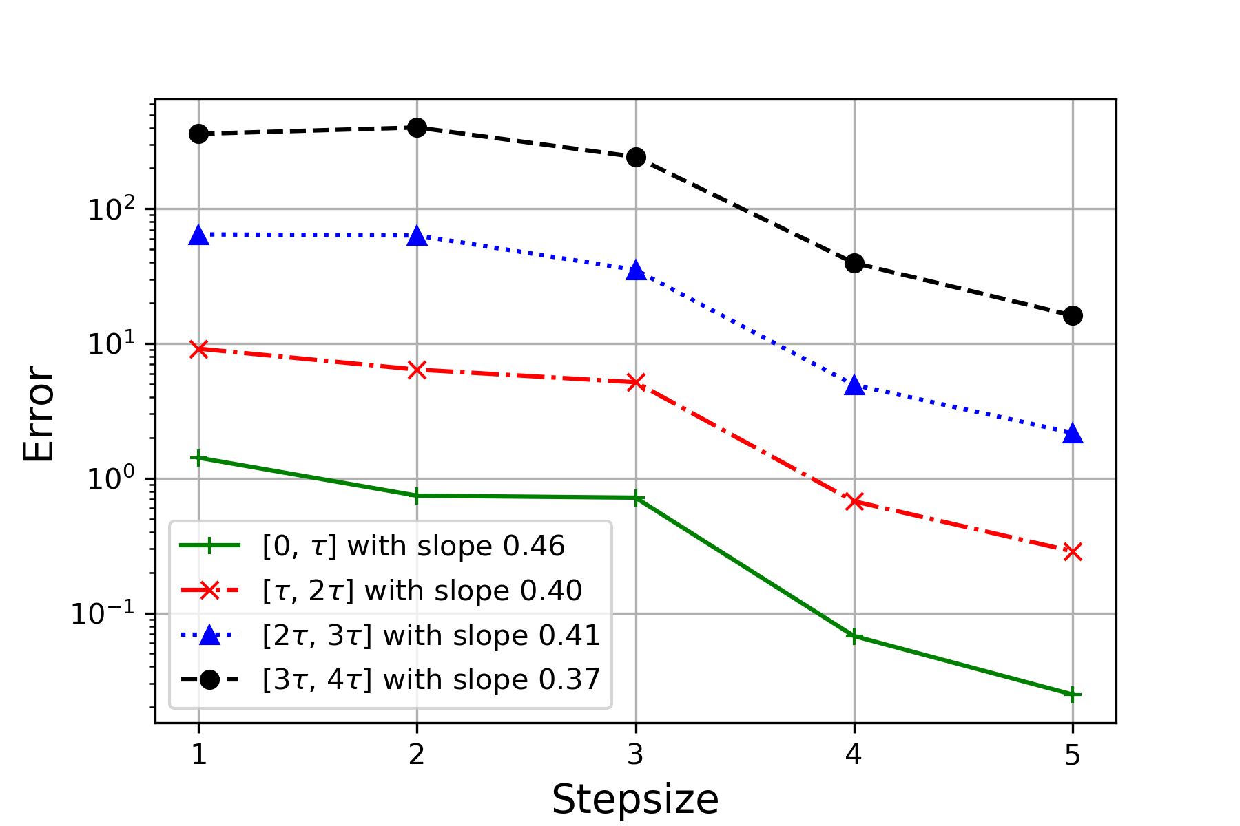
(a) $\alpha=0.1$.

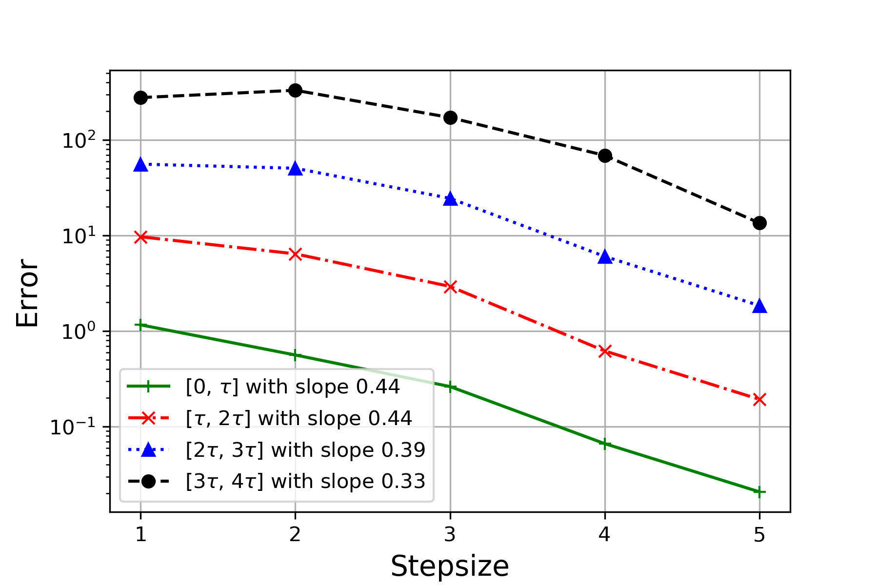
(b) $\alpha=0.5$.

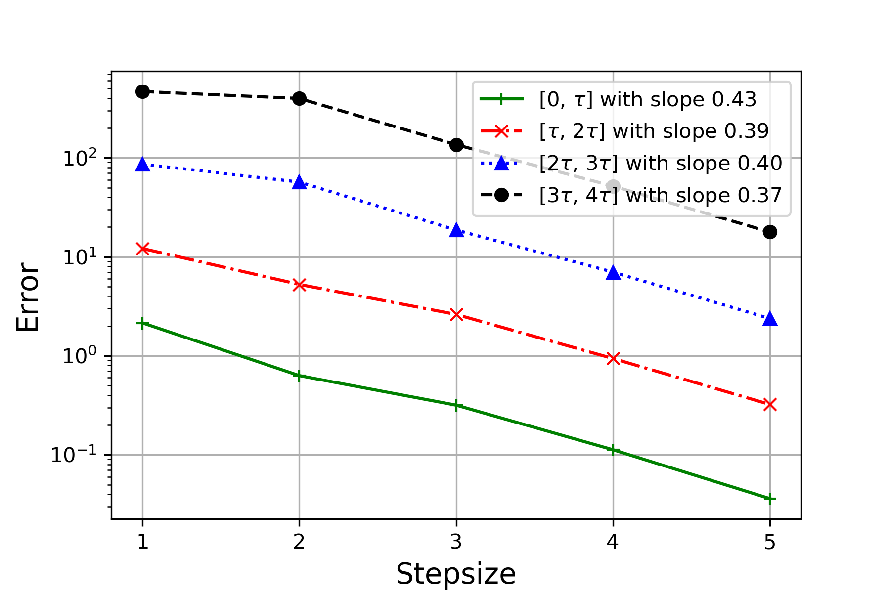
(c) $\alpha=1$.

Figure 1. Mean square errors slope for $\gamma=2.1$ and values of $\alpha=0.1,0.5,1$ in (5.1), using $M=10,P=100$.

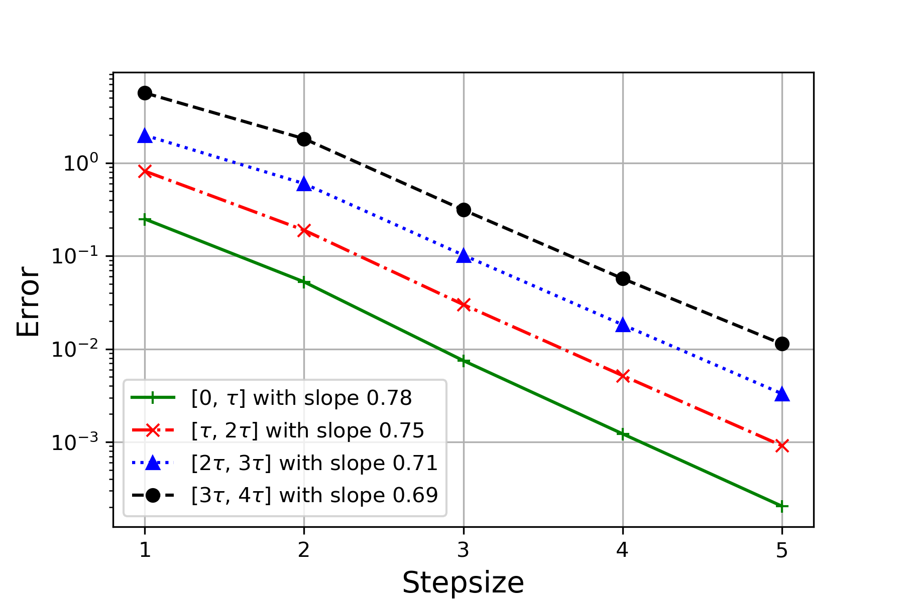
(a) $\alpha=0.1$.

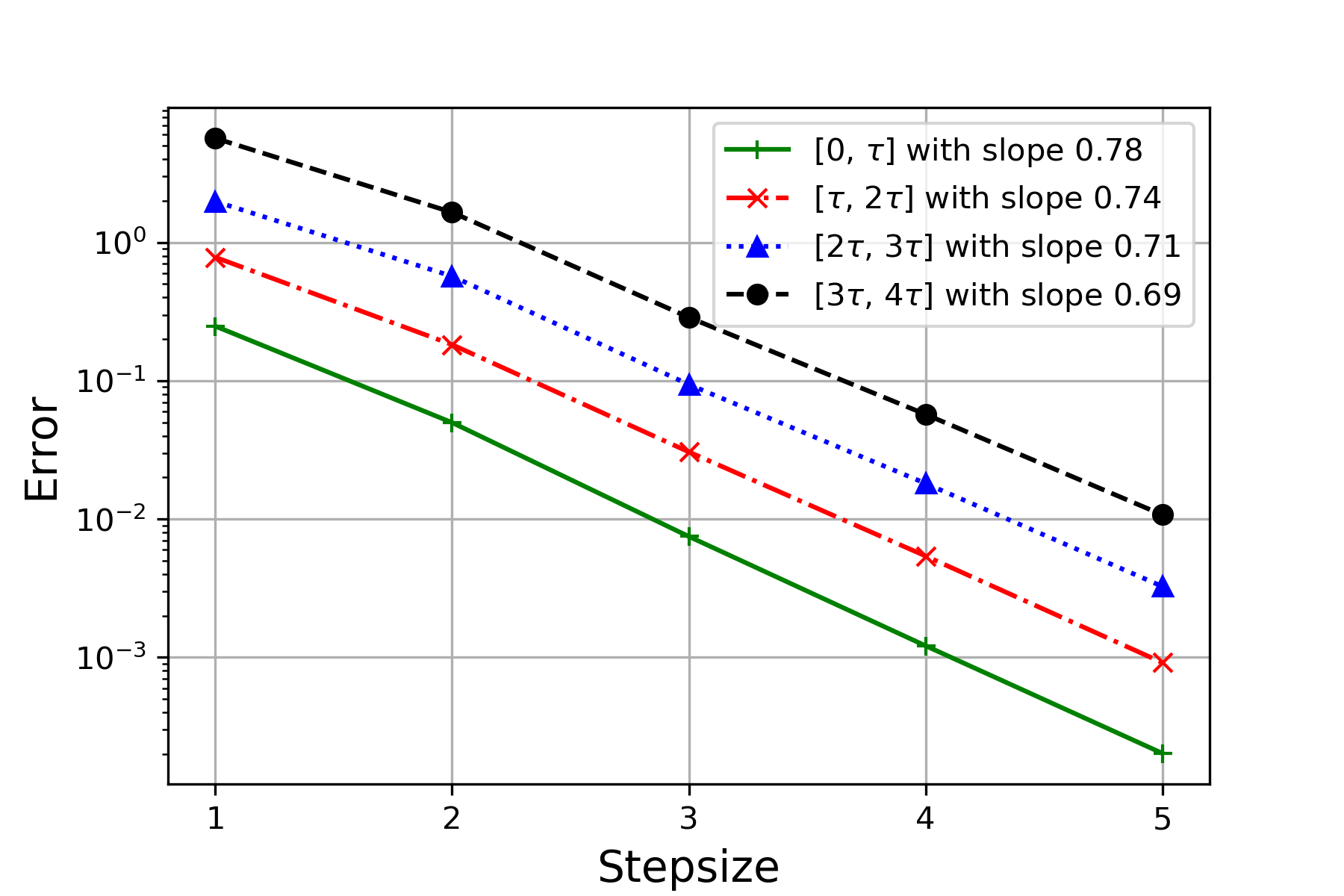
(b) $\alpha=0.5$.

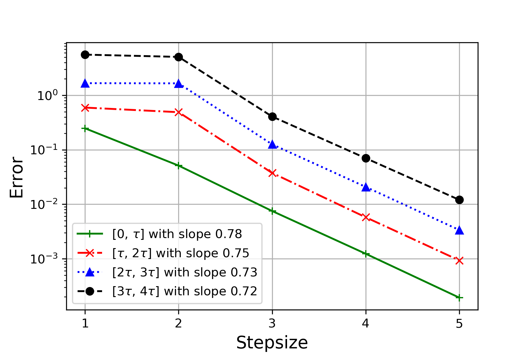
(c) $\alpha=1$.

Figure 2. Mean square errors slope for $\gamma=5$ and values of $\alpha=0.1,0.5,1$ in (5.1), using $M=10,P=100$.

Example 5.2.

In the following numerical tests we use (5.2) with parameters $M=10,P=100$. We fix the number of experiments $K=1000$ for each $N=2^{l}$, $l=3,\ldots,8$, and the reference solution is computed using $m=1000$; also, the horizon parameter is $n=5$.

We get the following results for $\gamma=2.1$:
letting $\alpha=0.1$, the negative mean square error slopes are $0.79$, $0.77$, $0.77$ and $0.78$. See Figure 3(a);
letting $\alpha=0.5$, the negative mean square error slopes are $0.79$, $0.78$, $0.77$ and $0.76$. See Figure 3(b);
letting $\alpha=1$, the negative mean square error slopes are $0.80$, $0.79$, $0.78$ and $0.77$. See Figure 3(c);
while, for $\gamma=5$:
letting $\alpha=0.1$, the negative mean square error slopes are $0.80$, $0.78$, $0.77$ and $0.76$. See Figure 4(a);
letting $\alpha=0.5$, the negative mean square error slopes are $0.79$, $0.79$, $0.78$ and $0.77$. See Figure 4(b);
letting $\alpha=1$, the negative mean square error slopes are $0.80$, $0.80$, $0.79$ and $0.78$. See Figure 4(c).

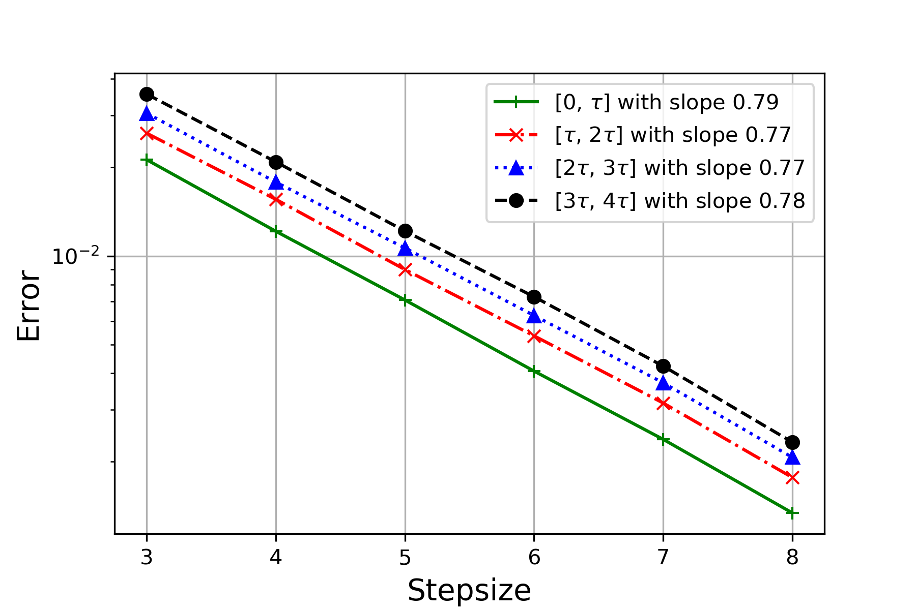
(a) $\alpha=0.1$.

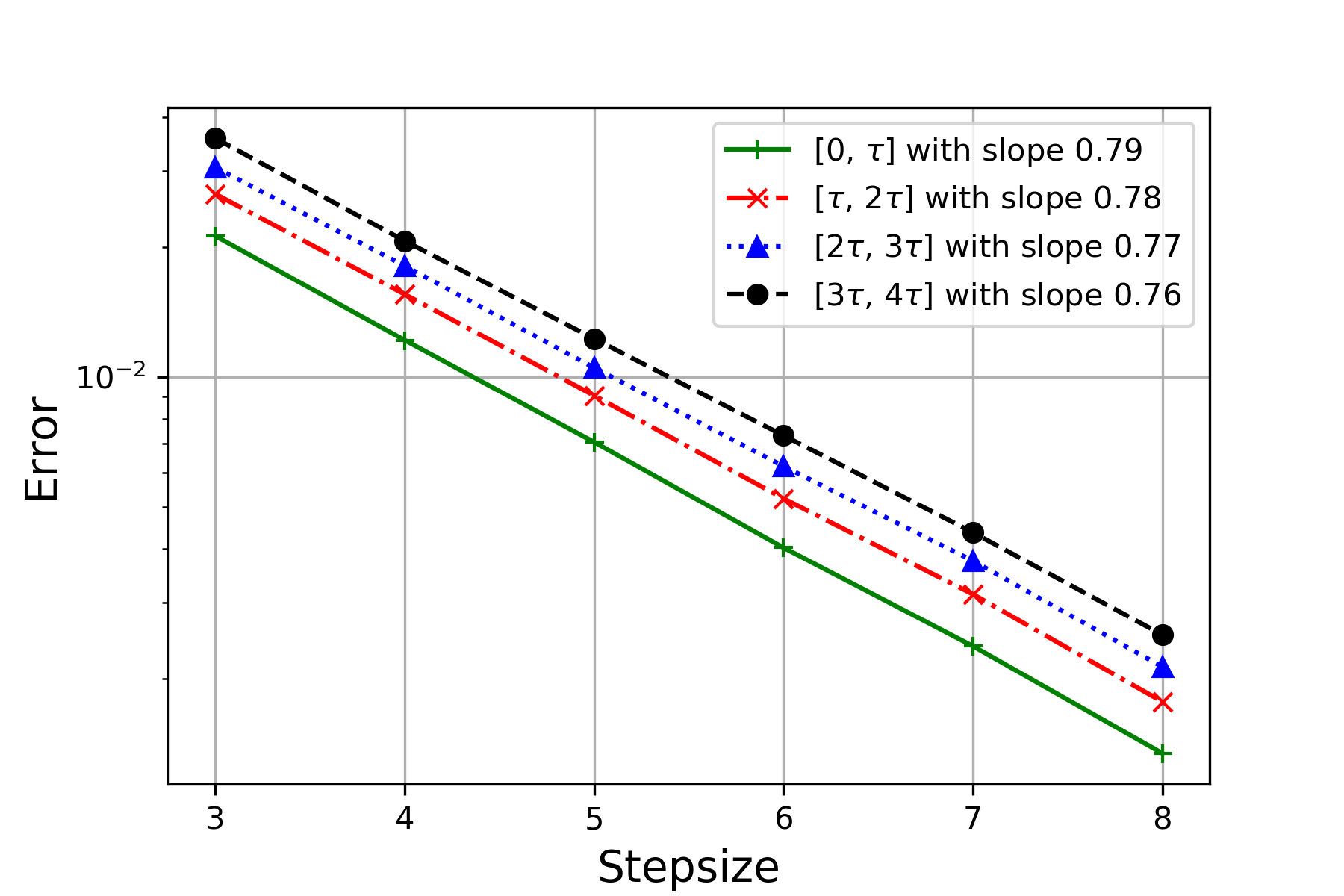
(b) $\alpha=0.5$.

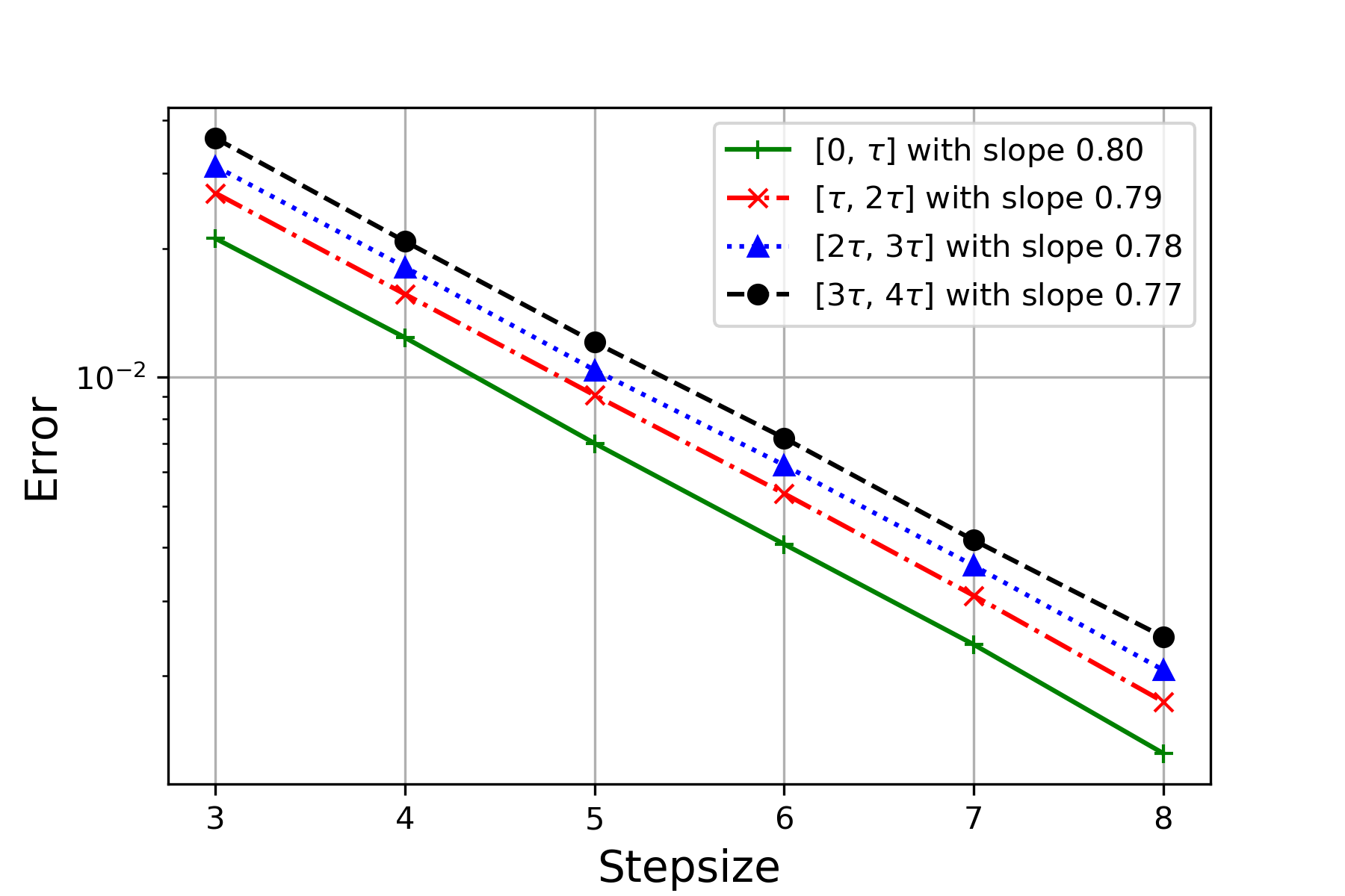
(c) $\alpha=1$.

Figure 3. Mean square errors slope for $\gamma=2.1$ and values of $\alpha=0.1,0.5,1$ in (5.2), using $M=10,P=100$.

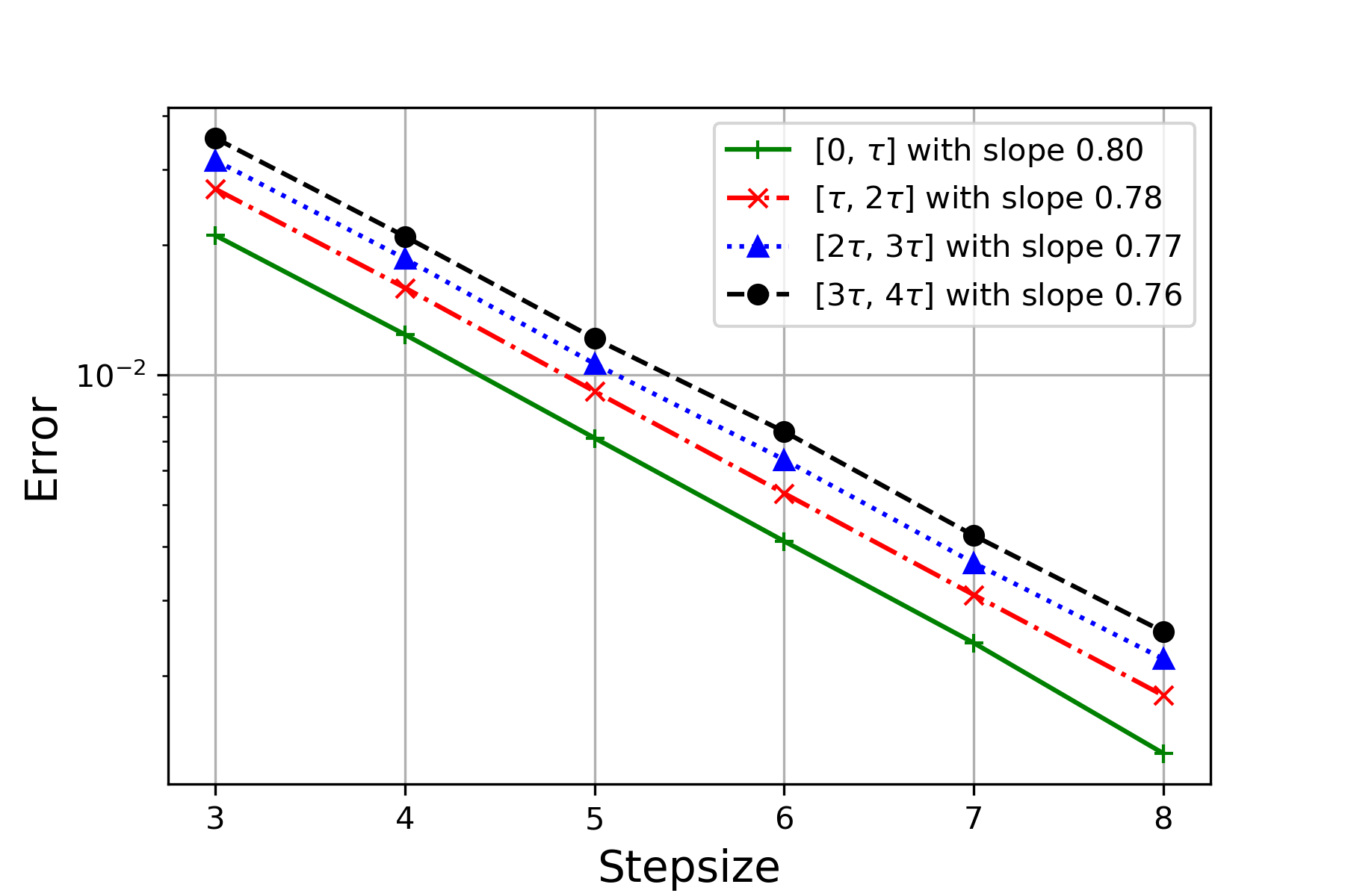
(a) $\alpha=0.1$.

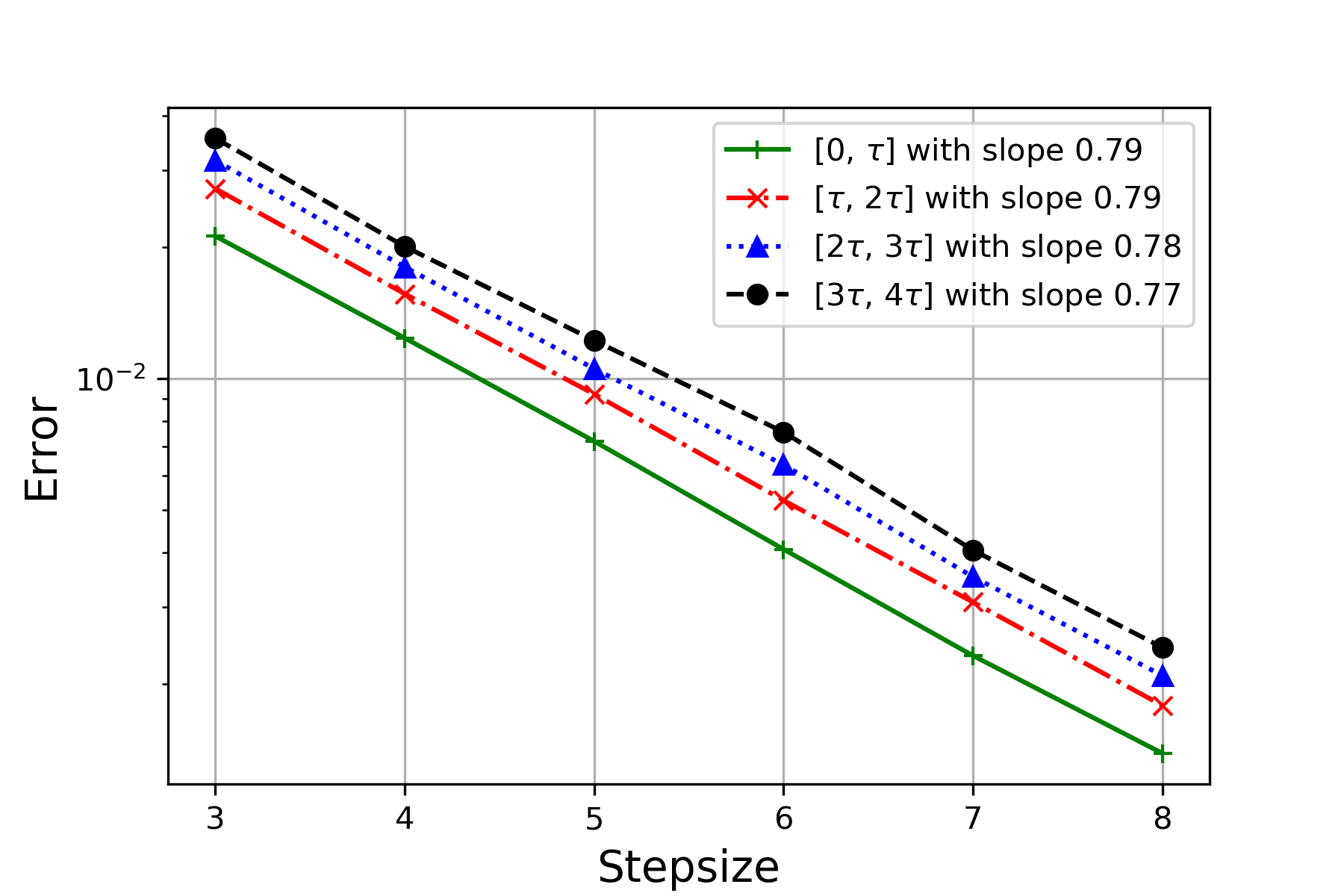
(b) $\alpha=0.5$.

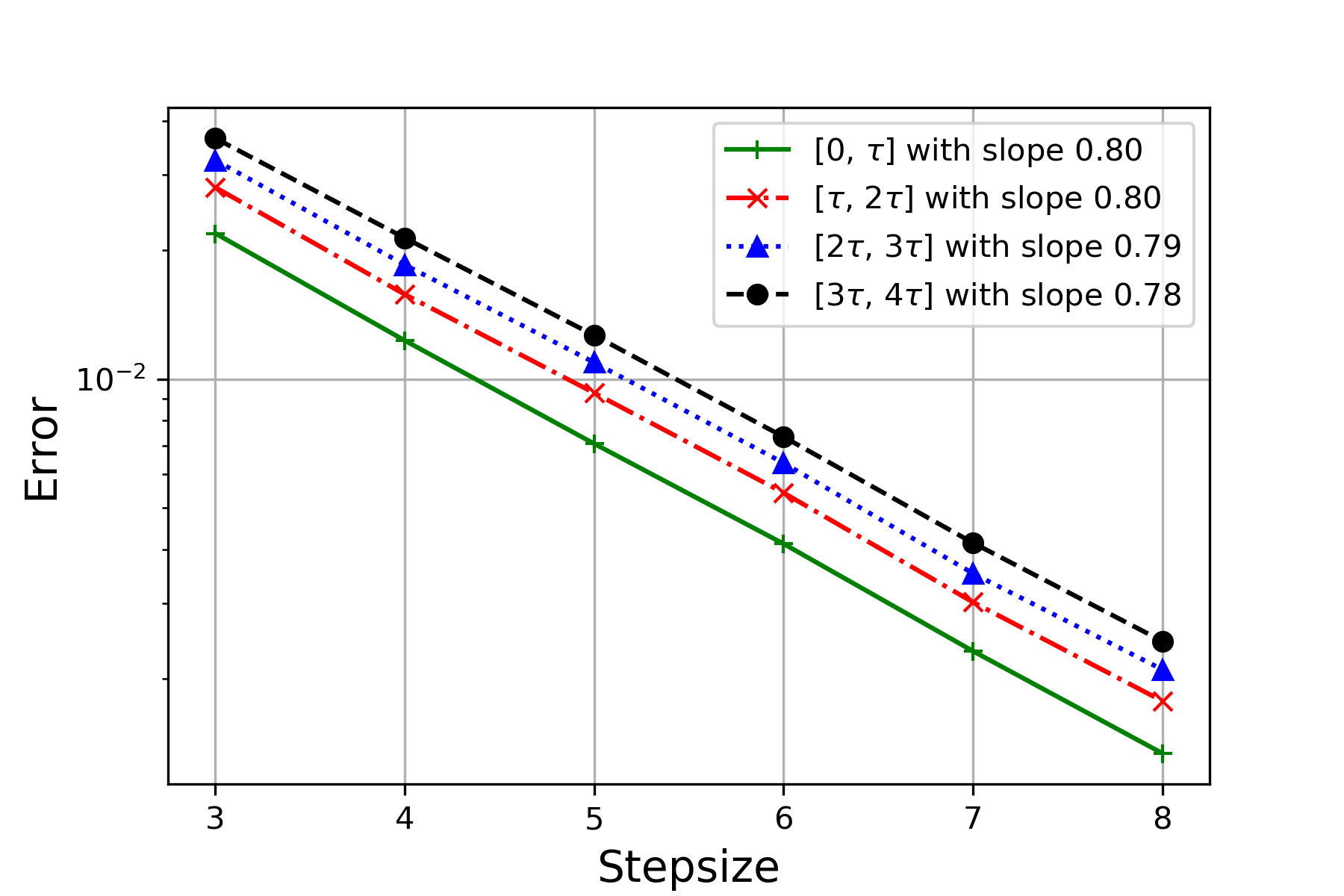
(c) $\alpha=1$.

Figure 4. Mean square errors slope for $\gamma=5$ and values of $\alpha=0.1,0.5,1$ in (5.2), using $M=10,P=100$.

Example 5.3.

From [12] we consider the following DDE

(5.4) $$\begin{cases}x^{\prime}(t)=3x(t-\tau)\sin(\lambda t),&t\geq 0,\\ x(t)=x_{0},&t\leq 0,\end{cases}$$

with $\tau=1$, $\lambda=2^{\nu}$ and $1\leq\nu\leq 16$. Thus, with our formalism, we have to consider the function

$$f(t,x,z)\mathrel{\mathop{:}}=3z\sin(\lambda t),$$

which satisfies assumptions (A1), (A2), (A3’). In this case the exact solution can be computed in closed form. Namely, by using the fact that for $j\geq 0$ and $t\in[j\tau,(j+1)\tau]$ it holds

(5.5) $$\phi_{j}(t)=\phi_{j-1}(j\tau)+3\int\limits_{j\tau}^{t}\phi_{j-1}(u-\tau)\sin(\lambda u)\mathrm{d}u.$$

In this experiment, we consider $t\in[0,2\tau]$, thus the true solutions over $[0,\tau]$ and $[\tau,2\tau]$ are therefore

• for $t\in[0,\tau]$

  (5.6) $$\phi_{0}(t)=x_{0}+3x_{0}\frac{1-\cos(\lambda t)}{\lambda},$$

• for $t\in[\tau,2\tau]$

  (5.7) $$\begin{split}\phi_{1}(t)=&\phi_{0}(\tau)-\big{(}\frac{9x_{0}}{\lambda^{2}}+\frac{3x_{0}}{\lambda}\big{)}(\cos(\lambda t)-\cos(\lambda\tau))+\frac{9x_{0}}{2\lambda}(t-\tau)\sin(-\lambda\tau)\\ &+\frac{9x_{0}}{4\lambda^{2}}(\cos(2\lambda t-\lambda\tau)-\cos(\lambda\tau)).\end{split}$$

Exact solutions for $\lambda=2^{\nu}$, $\nu=1,\ldots,9$ are depicted in Figure 5.

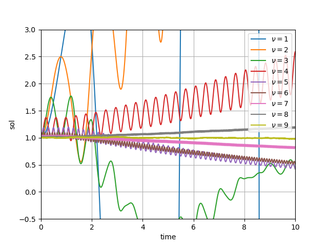
Figure 5. Solutions to problem (5.4).

We fix the number of experiments $K=1000$ for each $N=2^{l}$, $l=5,\ldots,10$, choose $x_{0}=1$. With $\nu=8$ the errors from both randomized Euler and Euler schemes are depicted in Figure 6, where the slopes are both beyond $1.00$ over $[0,\tau]$, and Euler method has a slower convergence over $[\tau,2\tau]$.

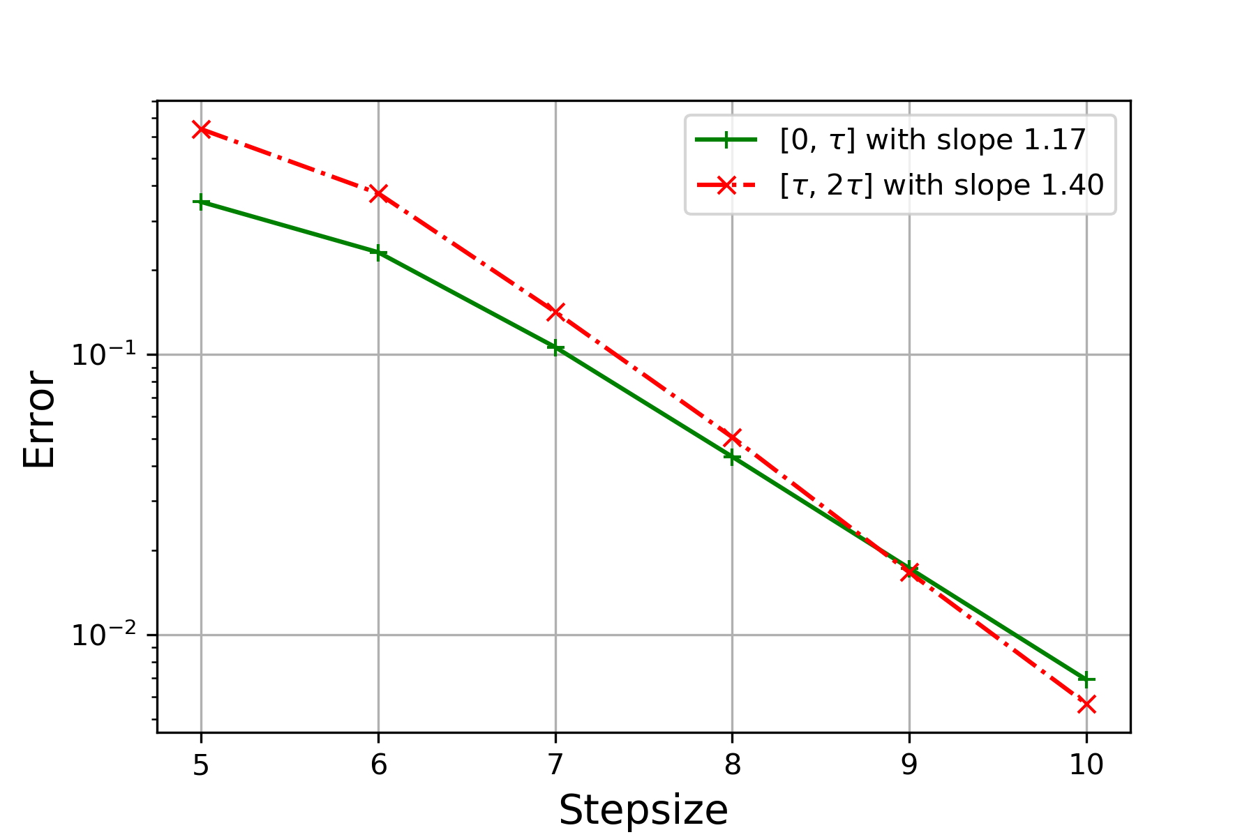
(a) Randomized Euler method

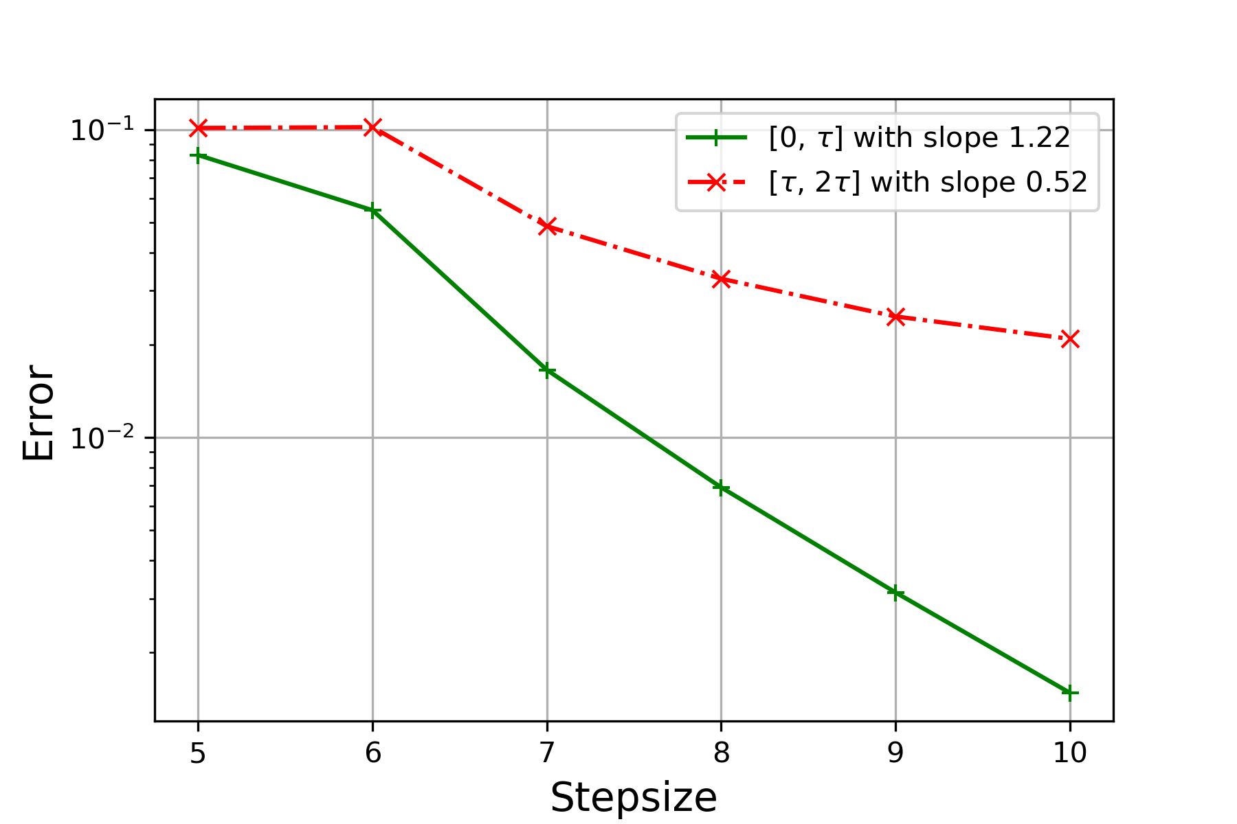
(b) Euler method

Figure 6. Error comparison between randomized Euler method and Euler method for Example 5.3 with $\nu=8$ over $[0,\tau]$ and $[\tau,2\tau]$.

Example 5.4.

Following the example in [15, Section 7] we consider the following DDE

(5.8) $$\begin{cases}x^{\prime}(t)=\sin{(\lambda_{1}t)}+x(t)+|x(t-1)|^{\alpha},&t\geq 0,\\ x(t)=1,&t\leq 0.\end{cases}$$

Thus, with our formalism, we have to consider the function

$$f(t,x,z)\mathrel{\mathop{:}}=\sin{(\lambda_{1}t)}+x+|z|^{\alpha},$$

which satisfies assumptions (A1), (A2), (A3’).
In the experiment, we set $\lambda_{1}=2^{9}\pi$ and $\alpha=0.2$. We compare the numerical solution of (5.8) by the randomized Euler scheme (2.4)-(2.5) and its classical counter-part over $[j\tau,(j+1)\tau]$, for $j\in\{0,1,2\}$ respectively, where $\tau=1$ in this example. We approximate the error by a Monte Carlo simulation with 1000 independent samples. Hereby, the reference solution is obtained using the randomized Euler scheme with a finer step size of $h_{\text{ref}}$ = $2^{-16}$.

In Figure 7, we plot the errors against the underlying step size, i.e., the number $i$ on the x-axis indicates the corresponding simulation is based on the step size $h=2^{-i}$ . The finest step size here is $2^{-10}$. The two sets of error data are fitted with a linear function via linear regression respectively, where the slope indicates the average order of convergence. It is noted that the classical Euler scheme does not begin to converge until $i=9$. The reason for this is, that for any coarser (equidistant) step size larger than $2^{-9}$ the classical Euler scheme cannot distinguish the term $|\sin(\lambda_{1}t)|$ from the zero function. In contrast, the randomized Euler method shows better results already for much coarser step sizes. Note that the experimental order of convergence is decreasing with $j$ for randomized Euler as expected (see the result for $\alpha<1$ in Theorem 4.2).

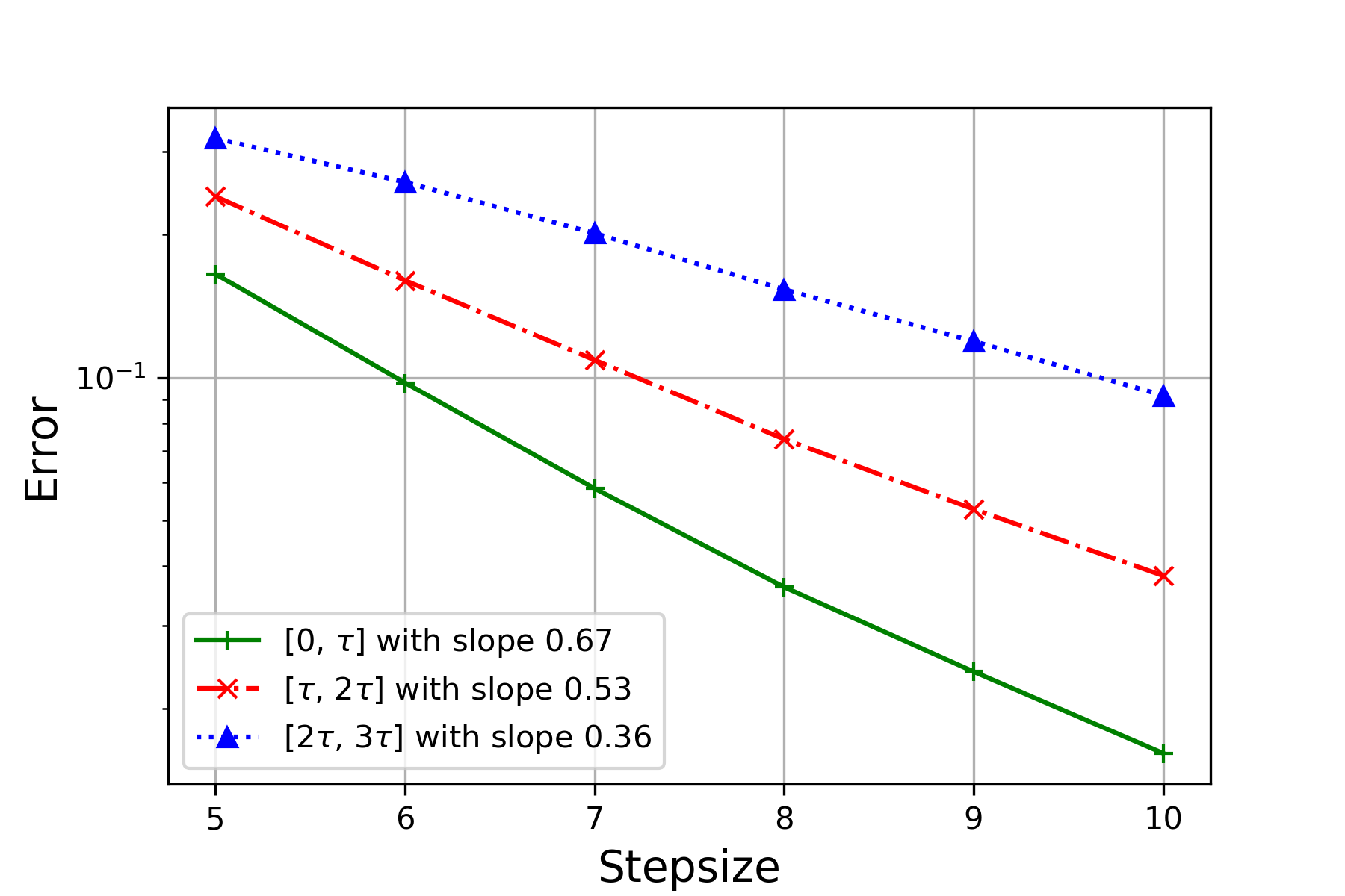
(a) Randomized Euler method

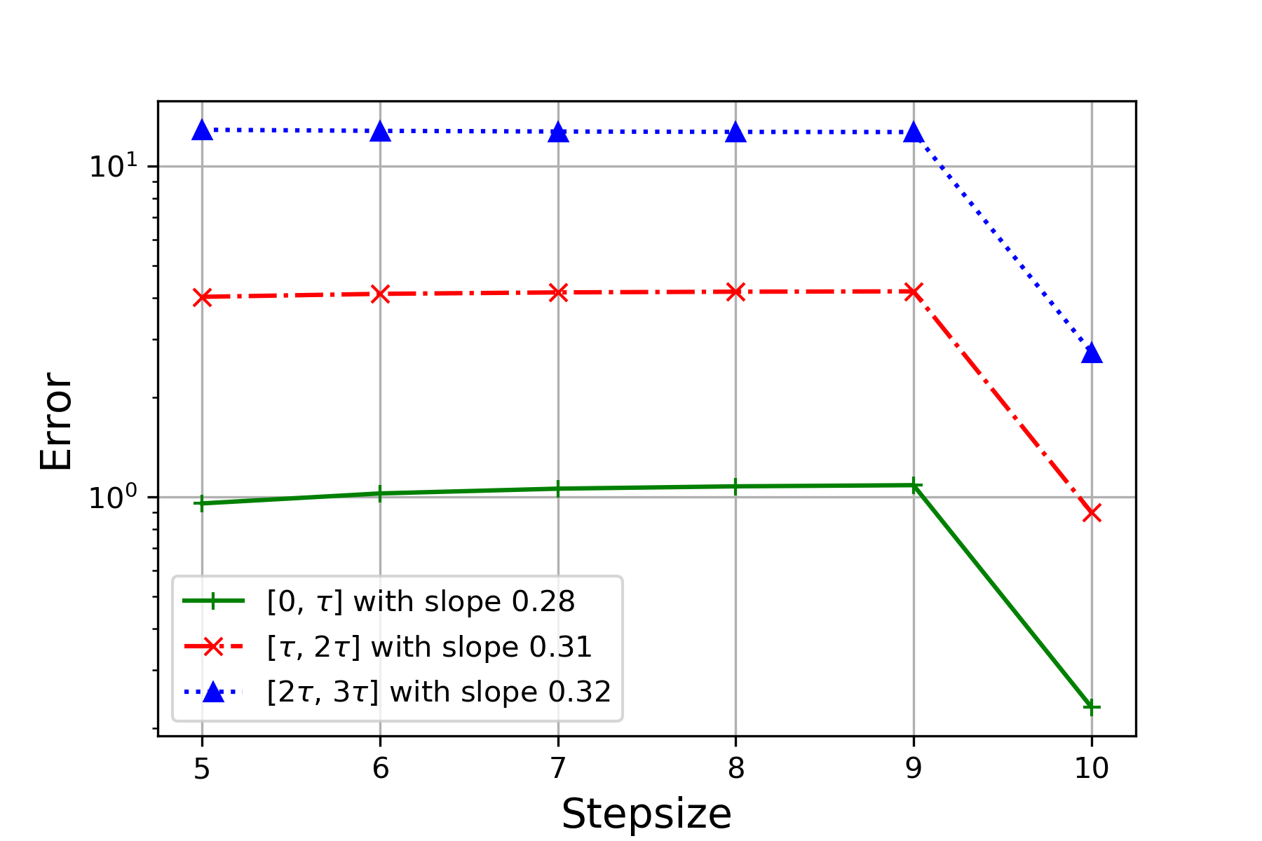
(b) Euler method

Figure 7. Error comparison between randomized Euler method and Euler method for Example 5.4 over $[0,\tau]$, $[\tau,2\tau]$ and $[2\tau,3\tau]$.

Example 5.5.

Finally we consider the inspiring example in (1.2) over $[0,2\tau]$ with $U_{0}=1$, where $Z(t)$ is given as one realization of Wiener process, and $a(x,z):=x+z$. Thus, with our formalism, we have to consider the function

$$f(t,x,z)\mathrel{\mathop{:}}=a(x+Z(t),z+Z(t-\tau))=x+Z(t)+z+Z(t-\tau),$$

which clearly satisfies assumptions (A1), (A2), (A3’).
In the experiment, we compare the numerical solution of (5.8) by the randomized Euler scheme (2.4)-(2.5) and its classical counter-part over $[j\tau,(j+1)\tau]$, for $j\in\{0,1\}$ respectively, where $\tau=2$ in this example. We approximate the error by a Monte Carlo simulation with 1000 independent samples. Hereby, the reference solution is obtained using the Euler scheme with a finer step size of $h_{\text{ref}}$ = $2^{-16}$. Note that the realization of Wiener process is generated on the time grid with stepsize $h_{\text{ref}}$ over $[0,3\tau]$, while $Z(t)=0$ for $t<0$. The whole path evaluation $Z(t)$ for $t\in[-\tau,3\tau]$ is obtained through piecewise linear interpolation.

In Figure 8, we plot the errors against the underlying step size, i.e., the number $i$ on the x-axis indicates the corresponding simulation is based on the step size $h=2^{-i}$. The finest step size here is $2^{-8}$. The two sets of error data are fitted with a linear function via linear regression respectively, where the slope indicates the average order of convergence. It is noted that the classical Euler scheme has a worse performance over $[2\tau,3\tau]$. The experimental orders of convergence from both methods are higher than the theoretical results shown in Theorem 4.2).

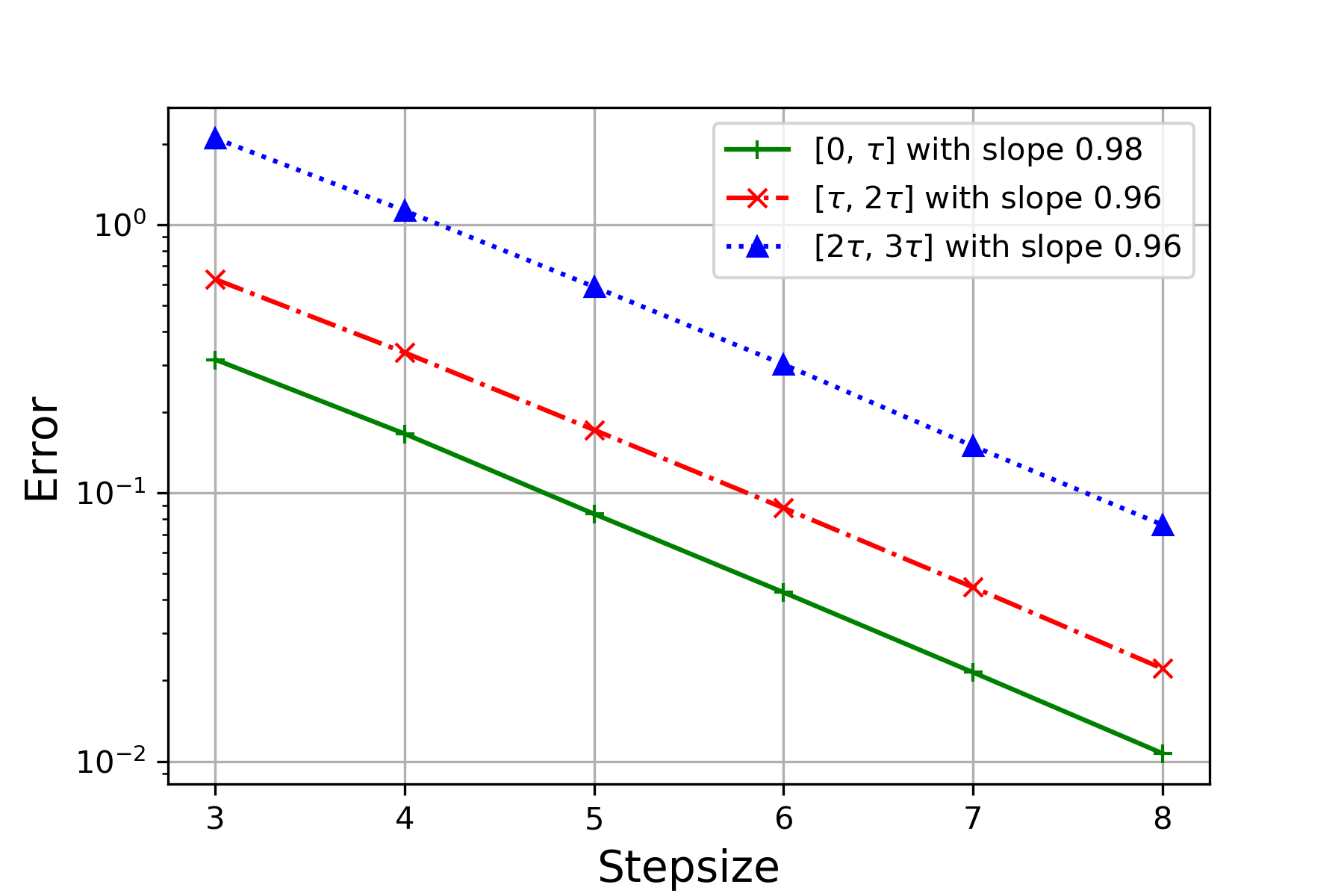
(a) Randomized Euler method

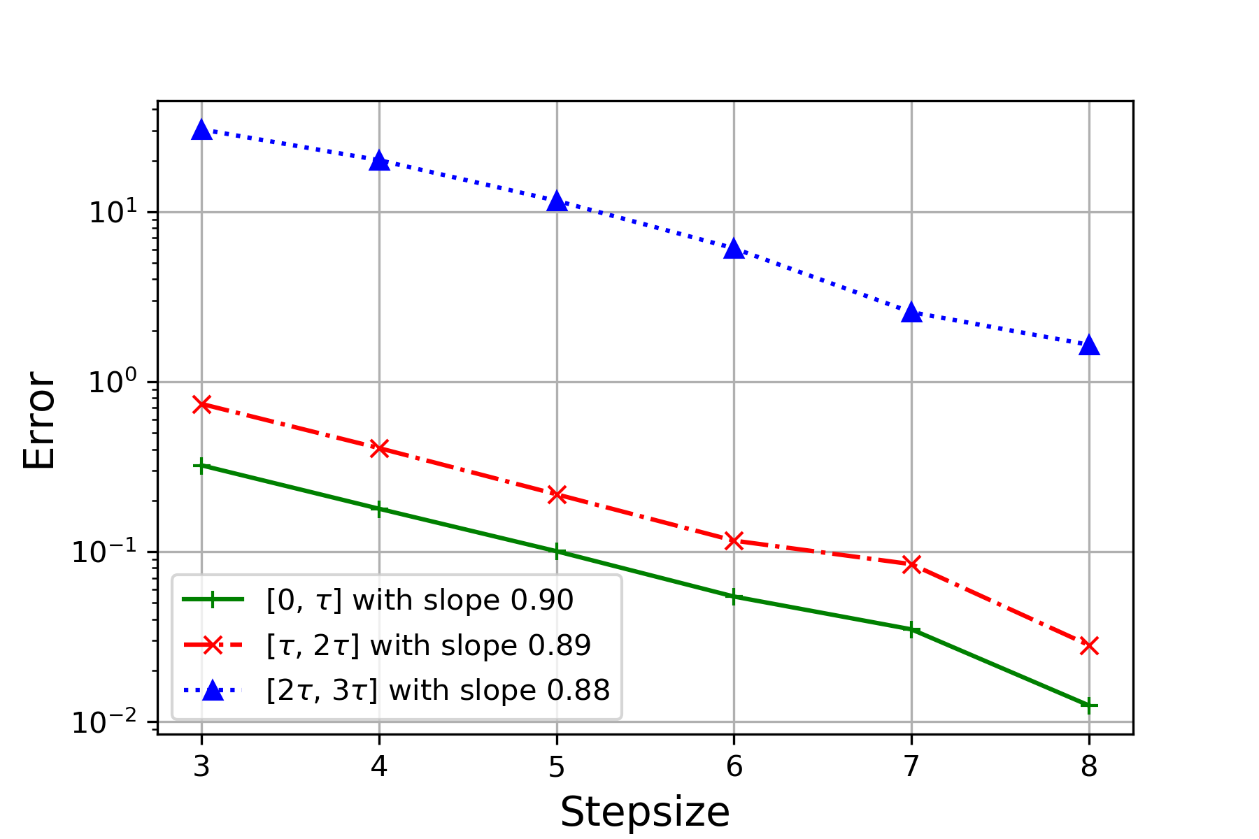
(b) Euler method

Figure 8. Error comparison between randomized Euler method and Euler method for Example 5.5 over $[0,\tau]$, $[\tau,2\tau]$ and $[2\tau,3\tau]$.

6. Conclusions

We investigated existence, uniqueness and numerical approximation of solutions of Carathéodory DDEs. In particular, we showed upper bound on the $L^{p}(\Omega)$-error for the randomized Euler scheme under global Lipschitz/Hölder condition (A3’). We conjecture however that the established upper error bound also holds under weaker local Lipschitz assumption. We plan to address this topic in our future work.

7. Appendix

We use the following result concerning properties of solutions of Carathéodory ODEs. It follows from [1, Theorem 2.12, pag. 252]. (Compare also with [14, Proposition 4.2].)

Lemma 7.1.

Let us consider the following ODE

(7.1) $$z^{\prime}(t)=g(t,z(t)),\quad t\in[a,b],\quad z(a)=\xi,$$

where $-\infty<a<b<+\infty$, $\xi\in\mathbb{R}^{d}$ and $g:[a,b]\times\mathbb{R}^{d}\to\mathbb{R}^{d}$ satisfies the following conditions

1. for all $t\in[a,b]$ the function $g(t,\cdot):\mathbb{R}^{d}\to\mathbb{R}^{d}$ is continuous,

2. for all $y\in\mathbb{R}^{d}$ the function $g(\cdot,y):[a,b]\to\mathbb{R}^{d}$ is Borel measurable,

3. there exists $K:[a,b]\to[0,+\infty)$ such that $K\in L^{1}([a,b])$ and for all $(t,y)\in[a,b]\times\mathbb{R}^{d}$

   $$\|g(t,y)\|\leq K(t)(1+\|y\|),$$

4. for every compact set $U\subset\mathbb{R}^{d}$ there exists $L_{U}:[a,b]\to\mathbb{R}^{d}$ such that $L_{U}\in L^{1}([a,b])$ and for all $t\in[a,b]$, $x,y\in U$

   (7.2) $$\|g(t,x)-g(t,y)\|\leq L_{U}(t)\|x-y\|.$$

Then (7.1) has a unique absolutely continuous solution $z:[a,b]\to\mathbb{R}^{d}$ such that

(7.3) $$\sup\limits_{t\in[a,b]}\|z(t)\|\leq(\|\xi\|+\|K\|_{L^{1}([a,b])})e^{\|K\|_{L^{1}([a,b])}}.$$

Moreover, if $K\in L^{p}([a,b])$ for some $p\in(1,+\infty]$, then for all $t,s\in[a,b]$

(7.4) $$\|z(t)-z(s)\|\leq\bar{K}|t-s|^{1-\frac{1}{p}},$$

where $\bar{K}=\|K\|_{L^{p}([a,b])}\cdot\Bigl{(}1+(\|\xi\|+\|K\|_{L^{1}([a,b])})e^{\|K\|_{L^{1}([a,b])}}\Bigr{)}$.

Proof.

By (G1), (G2), (G3) and by applying Theorem (2.12) from [1, pag. 252] to the set-valued mapping $F(t,x)=\{g(t,x)\}$, we get that (7.1) has at least one absolutely continuous solution. Moreover, any solution $z$ of (7.1) satisfies for all $t\in[a,b]$

(7.5) $$\|z(t)\|\leq\|\xi\|+\int\limits_{a}^{t}\|g(s,z(s))\|\,\mathrm{d}s\leq\|\xi\|+\|K\|_{L^{1}([a,b])}+\int\limits_{a}^{t}K(s)\|z(s)\|\,\mathrm{d}s$$

and by applying Gronwall’s lemma (see [18, pag. 22]) we get the estimate (7.3).

Let us consider the ball

(7.6) $$B_{0}=\{y\in\mathbb{\mathbb{R}}^{d}\ |\ \|y\|\leq(\|\xi\|+\|K\|_{L^{1}([a,b])})e^{\|K\|_{L^{1}([a,b])}}\},$$

which is a compact subset of $\mathbb{R}^{d}$. Let $z$ and $\tilde{z}$ are two solutions to (7.1). From the consideration above we know that $z(t),\tilde{z}(t)\in B_{0}$ for all $t\in[a,b]$. Hence, by (G4) applied to $U:=B_{0}$ we get that there exists non-negative $L_{U}\in L^{1}([a,b])$ such that for all $t\in[a,b]$

(7.7) $$\|z(t)-\tilde{z}(t)\|\leq\int\limits_{a}^{t}\|g(s,z(s))-g(s,\tilde{z}(s))\|\,\mathrm{d}s\leq\int\limits_{a}^{t}L_{U}(s)\cdot\|z(s)-\tilde{z}(s)\|\,\mathrm{d}s.$$

This and Gronwall’s lemma (see [18, pag. 22]) imply that $z(t)=\tilde{z}(t)$ for all $t\in[a,b]$.

Finally, for all $s,t\in[a,b]$ we get by the Hölder inequality that

(7.8) $$\|z(t)-z(s)\|\leq(1+\sup\limits_{a\leq t\leq b}\|z(t)\|)\int\limits_{\min\{t,s\}}^{\max\{t,s\}}K(u)\,\mathrm{d}u$$

(7.9) $$\leq(1+\sup\limits_{a\leq t\leq b}\|z(t)\|)\cdot\|K\|_{L^{p}([a,b])}\cdot|t-s|^{1-\frac{1}{p}}.$$

Hence, by (7.9) and (7.3) we get (7.4). ∎

Remark 7.2.

For the readers familiar with stochastic differential equations we stress that the existence and uniqueness of solution to (7.1) under the assumptions (G1)-(G4) can also be derived from [17, Proposition 3.28, pag. 187].

References

- [1] J. Andres and L. Górniewicz. Topological Fixed Point Principles for Boundary Value Problems, vol. I. Springer Science+Business Media Dordrecht, 2003.
- [2] A. Bellen and M. Zennaro. Numerical methods for delay differential equations. Oxford, New York, 2003.
- [3] T. Bochacik, M. Goćwin, P. M. Morkisz, and P. Przybyłowicz. Randomized Runge-Kutta method–Stability and convergence under inexact information. J. Complex., 65:101554, 2021.
- [4] T. Bochacik and P. Przybyłowicz. On the randomized Euler schemes for ODEs under inexact information. to appear in Numerical Algorithms, 2022.
- [5] N. Czyżewska, P. M. Morkisz, and P. Przybyłowicz. Approximation of solutions of DDEs under nonstandard assumptions via Euler scheme. https://arxiv.org/abs/2106.03731, 2022.
- [6] T. Daun. On the randomized solution of initial value problems. J. Complex., 27:300–311, 2011.
- [7] J. K. Hale. Theory of Functional Differential Equations. Applied Mathematical Sciences. Springer New York, 1977.
- [8] J. K. Hale and S. M. V. Lunel. Introduction to Functional Differential Equations. Springer-Verlag, New York, 1993.
- [9] S. Heinrich and B. Milla. The randomized complexity of initial value problems. J. Complex., 24:77–88, 2008.
- [10] A. Jentzen and A. Neuenkirch. A random Euler scheme for Carathéodory differential equations. J. Comp. Appl. Math., 224:346–359, 2009.
- [11] B. Kacewicz. Almost optimal solution of initial-value problems by randomized and quantum algorithms. J. Complex., 22:676–690, 2006.
- [12] R. Kainhofer. QMC methods for the solution of delay differential equations. Journal of Computational and Applied Mathematics, 155(2):239–252, jun 2003.
- [13] P. E. Kloeden and A. Neuenkirch. The pathwise convergence of approximation schemes for stochastic differential equations. LMS J. Comput. Math., 10:235–253, 2007.
- [14] R. Kruse and Y. Wu. Error analysis of randomized Runge–Kutta methods for differential equations with time-irregular coefficients. Comput. Methods Appl. Math., 17:479–498, 2017.
- [15] Raphael Kruse and Yue Wu. A randomized milstein method for stochastic differential equations with non-differentiable drift coefficients. arXiv preprint arXiv:1706.09964, 2017.
- [16] E. Novak. Deterministic and Stochastic Error Bounds in Numerical Analysis. Lecture Notes in Mathematics, vol. 1349, New York, Springer-Verlag, 1988.
- [17] E. Pardoux and A. Rascanu. Stochastic Differential Equations, Backward SDEs, Partial Differential Equations. Stochastic Modelling and Applied Probability. Springer International Publishing Switzerland, 2014.
- [18] E. Platen and N. Bruti-Liberati. Numerical Solution of Stochastic Differential Equations with Jumps in Finance. Stochastic Modelling and Applied Probability. Springer–Verlag Berlin Heidelberg, 2010.