Mock-integrability and stable solitary vortices

Abstract

Localized soliton-like solutions to a $(2+1)$-dimensional hydro-dynamical evolution equation are studied numerically. The equation is the so-called Williams-Yamagata-Flierl equation, which governs geostrophic fluid in a certain parameter range. Although the equation does not have an integrable structure in the ordinary sense, we find there exist shape-keeping solutions with a very long life in a special background flow and an initial condition. The stability of the localization at the fusion process of two soliton-like objects is also investigated. As for the indicator of the long-term stability of localization, we propose a concept of configurational entropy, which has been introduced in analysis for non-topological solitons in field theories.

I Introduction

Nonlinear integrable systems have exceptional properties in that they possess a sufficient number of integrals of motion, Painléve properties, reducibility into bilinear forms, and so on. They admit as a consequence localized solutions that retains their identity even under collision, the solitons. Solitons in nonlinear mathematical systems are eternally stable objects and simulate so many well-balanced phenomena in nature that a large amount of research has been done and is still underway Ablowitz and Segur (1981); Ablowitz and Clarkson (1991); T.Miwa (2000); Hirota (2004).

An archetypal example of integrable systems is the Korteweg-de Vries (KdV) equation, which describes the dynamics of surface waves propagating in one-dimensional shallow water. The dynamics of the KdV equation consist of a balance between dispersion and nonlinearity, and the system has an infinite number of integrals of motion and admits multi-soliton solutions. What characterizes the solitons in the KdV equation is their stability at collisions and exponentially dumping tails of each soliton. Several models of a generalization to the KdV equation into two-dimensional space as integrable systems are considered so far. One of these models is the Kadomtsev-Petviashvili (KP) equation, which describes shallow water waves propagating in two-dimensional space B.B.Kadomtsev and V.I.Petviashivilli (1970). The soliton solutions to the KP equation have a structure that dumps rapidly in one spatial direction and does not localize in the other direction, i.e., the KP solitons are extending in a two-dimensional plane with localization as a line. The system also has an infinite number of integrals of motion, the Lax formulation, the bilinear formulation, and the multi-soliton solutions Manakov et al. (1977). For that reason, the class of non-linear systems such as KdV and KP is referred to as the completely integrable systems.

Alternatively, there have been found various localized solutions to some integrable systems with rapidly decaying in all spatial directions, so-called dromions Davey and Stewartson (1974); Fokas and Santini (1990); Hietarinta (1990); Nishinari and Yajima (1994), topological multi-vortices Ishimori (1984), localized pulses in regularized-long-wave equations Kawahara et al. (1992), solitons in an extended Burgers equation Gao et al. (2022), and also several types of lump solitons Kaup (1981); Imai and Nozaki (1996); Zhang and Ma (2017); Zou et al. (2018), so on. They could explain various nonlinear phenomena of fluid dynamics of the atmosphere or ocean. In the case of the ocean, the waves are generated by the wind and are the response made by the water under the gravity or surface tension.

Among them, the Davey-Stewartson I (DSI) equation Davey and Stewartson (1974); Anker et al. (1978) provides a two-dimensional generalization of the non-linear Schrödinger equation and it possesses only one integral of motion in contrast to the completely integrable systems. Nevertheless, the DSI system has the Lax and the bilinear formulation. The lack of conserved quantities would be the characteristic that the system has lost, i.e., the fundamental feature of integrability as one-dimensional systems Boiti et al. (1995). In consequence, the solutions to the initial value problem to the DSI equation cannot be defined uniquely without fixing suitable boundary conditions. We notice here that the effects of the boundary conditions are the continuous supply of external “flow”. In this sense, the DSI equation does not belong to the completely integrable systems in its strictly meaning. Anyhow, the integrable systems in higher spatial dimensions that admit localized solutions in all directions are relatively rare.

In various ranges of mathematical physics, there are occasionally nonlinear systems that admit quasi-stable soliton-like solutions, although they do not have typical integrable structures, such as two-dimensional solitary Rossby-waves Larichev and Reznik (1976) or solitons in an inhomogeneous plasma Hasegawa and Mima (1978); Hasegawa et al. (1979). Such drift-wave solitons are a typical example of a weak-integrable system where metastable solutions are observed though no concrete analytical methods exist. An illustration is the Zakharov-Kuznetsov (ZK) equation Zakharov and Kuznetsov (1974) originally introduced to describe ion-acoustic waves in magnetized plasma. The ZK equation is a three-dimensional generalization of the KdV equation and its two-dimensional analogue is given as

$$\frac{\partial\phi}{\partial t}+\nabla^{2}\frac{\partial\phi}{\partial x}+2\phi\frac{\partial\phi}{\partial x}=0\,,$$ (1)

where the Laplacian is $\nabla^{2}:=\partial_{x}^{2}+\partial_{y}^{2}$. This equation also appears in some parts of physics such as a behavior of thin liquid film Petviashvili (1981); Toh et al. (1989); Melkonian and Maslowe (1989), the solitary Rosby-waves V.I.Petviashvili (1980), and vortex in the drift waves in the three-dimensional plasma Nozaki (1981), so it is continuously studied Xu and Shu (2005); Lannes et al. (2013); Klein et al. (2021) with some extensions. In the two-dimensional ZK equation (1), the nonlinear term is similar to the KdV equation and we refer to this nonlinearity as scalar nonlinearity. This equation has a rapidly decaying localized solution with cylindrical symmetry obtained numerically Iwasaki et al. (1990), whose behavior under collision is shown to be soliton-like in certain conditions due to the scalar nonlinearity. Despite the two-dimensional ZK equation (1) possessing quasi-soliton solutions, the system has only a finite number of integrals of motion, thus it cannot be identified as a completely integrable system. Note that the single soliton exhibits a certain long-life (longevity) during the long-term evolution. Though the analysis of longevity seems critical to understand the stability of the solution, no rigorous research concerning the long-term dynamical evolution of (1) exists so far.

In this paper, we draw attention to a nonlinear system in two spatial dimensions that are non-integrable and admit sufficiently localized and quasi-stable solutions. Collisions of traveling waves and isolated vortices are frequent phenomena in nature, observed both in the atmosphere and in the ocean. The dynamics of those familiar phenomena, and especially the behavior of long-lived, large-scale isolated vortices such as “the Great Red Spot (GRS)” of Jupiter in the atmosphere, “the Naruto whirlpools” of Japan’s coast in the ocean, have been of interest to many people. Therefore a lot of studies have been done so far Charney and Flierl (1981); Bouchet and Venaille (2012); Constantin (2009); Constantin and Henry (2009); Constantin (2011); Ibragimov et al. (2013); Ibragimov and Ibragimov (2013); Ibragimov and Lin (2017); Nezlin and Sutyrin (1989); Nezlin et al. (1993). We consider a similar non-linear system to the ZK equation (1) that appears in the geophysical fluid dynamics of the atmosphere, or ocean, on a rotating planet, including additional non-linearity and non-autonomous terms. It is an intermediate geostrophic equation for vorticity where the horizontal scales of the phenomena are smaller than the Rossby deformation radius. The equation is introduced first to explain the very long life of Jupiter’s GRS and so-called Williams-Yamagata-Flierl (WYF) equation Charney and Flierl (1981); Williams and Yamagata (1984), or simply IG (Intermediate Geostrophic) equation, for the stream function $\eta$ of a fluid. The equation in its normalized form is

$$-\frac{\partial\eta}{\partial T}+\nabla^{2}\frac{\partial\eta}{\partial x}+2\eta\frac{\partial\eta}{\partial x}-2y\frac{\partial\eta}{\partial x}+2J[\eta,\nabla^{2}\eta]=0\,,$$ (2)

which describes behavior of the vortex in a long time scale $T$. The last term, the Jacobian is defined as $J[A,B]:=\partial_{x}A\partial_{y}B-\partial_{y}A\partial_{x}B$ which represents the geostrophic advection of vorticity in the words of fluid dynamics, and we refer to it as the vector nonlinear term. The WYF equation (2) is derived from the shallow water $\beta$-plane model governing the stream function, or vorticity, of fluid under the influence of Coriolis force in a particular parameter range. The derivation is given in Appendix A. The pioneer work Williams and Yamagata (1984) shows that a vortex, i.e., a well-localized solution given by Gaussian initial shape, is sufficiently robust in a particular situation, and two distinct vortices merge into a single vortex, unlike soliton collisions. The vector nonlinear term contributes to the shape-keeping of the localized solutions in not a similar manner to the soliton systems, so the merging phenomena of the multi-vortices are the consequence of the cooperation of the scalar and the vector nonlinearities. We remark that this type of nonlinearity also appears in the Charney-Hasagawa-Mima equation Charney (1963); Hasegawa and Mima (1978); Hasegawa et al. (1979), which describes the drift waves in magnetized plasma, and also the geophysical flows in the $\beta$-plane at a different parameter range to the WYF equation. It is obvious that the varieties of nonlinearity increase as the spatial dimensions get larger, such as the vector nonlinearity appeared in the case of the WYF equation. We expect that the interplay between those various types of nonlinearity plays significant role in the formation and the stability of higher-dimensional solitons and soliton-like objects.

We focus on here the origin of the longevity of the single vortex solutions to the equation under the influence of this complicated nonlinearity together with external forces, i.e., the background shear flow given with non-autonomous terms. This paper investigates a modified WYF equation with, so-called the variable-coefficient form  Calogero and Degasperis (1978); Brugarino and Pantano (1980); Joshi (1987); Hlavatỳ (1988); Brugarino and Greco (1991); Gao and Tian (2001); Kobayashi and Toda (2005, 2006) that implements the effect of background shear flows in the equation. The explicit form is given in Section II, Eq.(15). We will find that the vortices secure eternal long-life in certain circumstances rather than expected from the previous works. In the present work, although the WYF equation is not integrable in any sense, we demonstrate that a steady external force is crucial to the stability of the soliton-like objects, i.e., vortices in two-dimensions. Those effects are included in the dynamical equations as non-autonomous terms, which are absent in ordinary soliton systems. We argue that the soliton-like stable, or very long-life objects appear occasionally as a consequence of those “mock-integrability”. In connection with this, we should remind the case of the DSI equation, in which there exist a suitable boundary condition for each soliton-like object.

The above non-integrable localized objects have some similarities with solitons in field theoretical models such as the $Q$-ball or the oscillon. The oscillon is a non-topological soliton in a scalar field theory with no explicit integrability. Typically, the oscillon has a bell shape that oscillates sinusoidally in time and has an extreme long life in some particular conditions Honda and Choptuik (2002). The oscillon was discovered in the seventies of the last century by Bogolyubsky and Makhankov Bogolyubsky and Makhankov (1976) and later revisited by Gleiser (1994); Copeland et al. (1995); Fodor et al. (2008, 2009). A notable feature is that the lifetime of the oscillons is strongly affected by the size of the initial configuration which may be common in the several quasi-integrable, or mock-integrable systems. We shall examine this issue: the initial condition dependency for longevity. For the analysis in the stability of localized object in field theory, an indirect method may be efficient for the estimation of the lifetime occasionally. Among them, the so-called configurational entropy is a quite promising candidate for understanding the stable nature of the localized objects Gleiser and Stamatopoulos (2012). For an attempt of this concept into fluid mechanical systems, we apply it for the analysis of the longevity of the vortices in the WYF equation. We expect that a criterion of the longevity of quasi-integrable vortices in the fluid dynamics would be given in the context of such information theoretical content.

This paper is organized as follows. In Section II we shall describe the model, including a thorough discussion of the close relation with several quasi-integrable systems such like the Zakharov-Kuznetsov equation or the Davey-Stewartson equation. The conservation nature of the model is also given in this section. Section III presents the numerical solutions of the model. Conclusions and remarks are presented in the last Section.

II Non-integrable models in steady background effects

In this section, we introduce the ZK and the WYF equations in detail for the subsequent analysis. As mentioned above, they are generalizations of the KdV equations into two-spatial dimensions.

II.1 Zakharov-Kuznetsov equation

The Zakharov-Kuznetsov equation originally was the model in three dimensions of plasma with a uniform magnetic field Zakharov and Kuznetsov (1974). The majority of the subsequent works, however, have been done for the two-dimensional analogue of the model Petviashvili and Yan’kov (1982); Iwasaki et al. (1990); Klein et al. (2021), which is defined as

$$\frac{\partial\phi}{\partial t}+2\phi\frac{\partial\phi}{\partial x}+\frac{\partial}{\partial x}(\nabla^{2}\phi)=0\,.$$ (3)

The model possesses meta-stable isolated solutions which enjoy the solitonic properties. The single soliton is stable in dynamical sense, and the two solitons with same height scatter without merging as in the KdV solitons. However, in the scattering of the two solitons with dissimilar height, the taller soliton becomes taller while the shorter one turns out to be shorter and radiates ripples Iwasaki et al. (1990). The stability of the solutions seem to rely on underlying KdV dynamics, especially the conserved quantities.

The equation possesses the solutions propagating in a specific direction with uniform speeds. Here we set the direction in the positive $x$ orientation with the velocity $c$, namely assuming $\phi=\Phi(x-ct,y)$. Plugging it into (3) we obtain

$$\nabla^{2}\Phi=c\Phi-\Phi^{2}\,,$$ (4)

where $\nabla^{2}=\partial_{\tilde{x}}^{2}+\partial_{y}^{2}$ and $\tilde{x}=x-ct$. A steady progressive exact wave solution is of the form

$$\Phi_{c}^{\rm rec}=\frac{3c}{2}{\rm sech}^{2}\biggl{[}\frac{\sqrt{c}}{2}(\tilde{x}\cos\theta+y\sin\theta)\biggr{]},$$ (5)

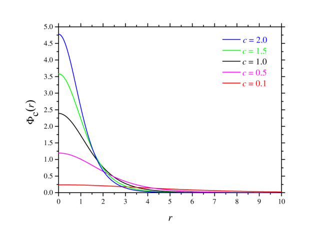
where the $\theta$ is a given inclined angle of the solution. From this form, it is easy to see that the solution is just a trivial embedding of the KdV soliton into two spatial dimensions. Here we would like to find the solutions to (3) keeping circular symmetry other than (5). In order to find it, we introduce cylindrical coordinate and rewrite the equation as

$$\frac{1}{r}\frac{d}{dr}\biggl{(}r\frac{d\Phi_{c}}{dr}\biggr{)}=c\Phi_{c}-\Phi_{c}^{2}\,,~{}~{}~{}~{}\Phi_{c}:=\Phi_{c}(r)\,,$$ (6)

where $r:=\sqrt{\tilde{x}^{2}+y^{2}}$. We are able to find a family of solutions to (6) with the boundary condition $\Phi_{c}\to 0$ as $r\to\infty$ in terms of a simple numerical study. The solutions form one parameter family of $c$ such as $\Phi_{c}(r):=cF(\sqrt{c}r)$. The result is shown in Fig.1. As is expected, the solution propagate in positive $x$ direction without any dissipation because of the character from the KdV like property.

Although the ZK equation (3) has the soliton-like solutions given above, the equation admits only a finite number of integrals of motion as shown in Kuznetsov et al. (1986), which are

$$M:=\int M(y)dy=\int\phi dxdy,\ M(y):=\int\phi dx,$$ (7)

$$P:=\int\frac{1}{2}\phi^{2}dxdy\,,$$ (8)

$$H:=\int\biggl{[}\frac{1}{2}(\nabla\phi)^{2}-\frac{1}{6}\phi^{3}\biggr{]}dxdy\,,$$ (9)

$$\bm{I}:=\int\bm{r}\phi dxdy-t\bm{e}_{x}\int\frac{1}{2}\phi^{2}dxdy\,,$$ (10)

where $\bm{r}$ and $\bm{e}_{x}$ are the two-dimensional position vector and the unit vector in the $x$-direction. Here $M$ is interpreted as the “Mass” of the solution, and $M(y)$ itself is conserved similarly to the KdV equation, respectively. We, therefore, conclude that the ZK equation is not an integrable system in the manner of ordinary soliton equations.

Figure 1: The circularly symmetric solutions of the ZK equation (3), which are quasi solitary wave solutions with the wave velocity $c$.

II.2 Intermediate geostrophic regime and Williams-Yamagata-Flierl equation

Several classes of geophysical fluid dynamics in two-dimensional approximation have been studied: the quasi-geostrophic (QG; small-scale), the planetary geostrophic (PG; long-scale) and intermediate geostrophic (IG; medium-scale) motions. For the IG regime, Williams and Yamagata proposed the governing equation for the vortices on the planetary atmosphere with the zonal currents, which are obtained from the standard shallow water system on the $\beta$-plane of coordinates $x,y$ Charney and Flierl (1981); Williams and Yamagata (1984). The equation is defined as

$$\frac{\partial\eta}{\partial T}-\frac{E}{S}\eta\frac{\partial\eta}{\partial x}-S\frac{\partial}{\partial x}(\nabla^{2}\eta)+2y\frac{\partial\eta}{\partial x}+EJ[\nabla^{2}\eta,\eta]=0\,,~{}~{}~{}~{}\eta:=\eta(x,y,T)\,,$$ (11)

where the Jacobian $J[A,~{}B]:=\partial_{x}A\partial_{y}B-\partial_{y}A\partial_{x}B$ and the Laplacian $\nabla^{2}:=\partial_{x}^{2}+\partial_{y}^{2}$. Here, the long time scale $T$ is related with the standard time coordinate $t$ as $T:=\hat{\beta}t,~{}~{}\hat{\beta}\ll 1,$ and it denotes the slow time coordinate that describes the long-term evolution of the vortices, see Appendix A. As the authors of Williams and Yamagata (1984) numerically shown, the equation (11) have a Gaussian shaped vortex solutions supposed to simulate a candidate for Jupiter’s red spot, which is considered to be an anti-cyclonic vortex. Though the results were sound, the discussions lack the mathematical discussions for the governing equation, i.e., scope of how the solutions are to be stable in terms of effects of the nonlinearity and the background shear flow. In particular, we will analyze here the nonlinear evolution equation under the influence of numerous background, or external flows, given in (11). We confirm that the equation (11) has well-localized solutions with sufficient longevity like solitons in completely integrable systems as mentioned in Introduction.

Figure 2:  Long-term simulation of the profile of the vortex $\eta(x,y,T)$ in $(f_{0},f_{1})=(0.0,1.2)$ for the iteration number: (a) $0$, (b) $1004\times 10^{4}$, (c) $4999\times 10^{4}$, (d) $9991\times 10^{4}$, respectively. We chose the time where the vortex is located at around the middle of the computational area. The initial condition is the circular symmetric Gaussian: $\xi_{\rm init}=3.0\times\exp\{-x^{2}-(y-1)^{2}\}$.

Figure 3:  Long-term simulation of the profile of the vortex $\eta(x,y,T)$ in $(f_{0},f_{1})=(0.0,1.2)$ for the iteration number: (a) $0$, (b) $1005\times 10^{4}$, (c) $5011\times 10^{4}$, (d) $9999\times 10^{4}$, respectively. The initial condition is the ZK profile of $c=1$ (see Fig.1).

In (11), the parameters $E$ and $S$ are of $O(1)$, which defines the scales of the vortices. Mathematically they can be removed with redefinition of the field and the coordinate such as

$$\eta\to\eta^{\prime}=\frac{1}{2}S^{-2/3}E\eta\,,~{}~{}~{}~{}x\to x^{\prime}=S^{-1/3}x\,.$$ (12)

The equation (11) reduces to

$$\frac{\partial\eta}{\partial T}-2\eta\frac{\partial\eta}{\partial x^{\prime}}-\frac{\partial}{\partial x^{\prime}}(\nabla^{\prime 2}\eta)+2y\frac{\partial\eta}{\partial x^{\prime}}+2J[\nabla^{\prime 2}\eta,\eta]=0\,.$$ (13)

Henceforth, we omit the prime for simplicity. As shown in Williams and Yamagata (1984), the WYF equation (11) has anti-cyclonic ($\eta>0$) Gaussian shaped vortex solutions when the appropriate background flow, or zonal currents, $u^{0}(y)$ are applied. For implementing the effect, we introduce a new variable

$$\xi(x,y,T):=\eta(x,y,T)+\int^{y}_{0}u^{0}(y^{\prime})dy^{\prime}\,.$$ (14)

Substituting this into (13), we obtain

$$\frac{\partial\xi}{\partial T}-2\xi\frac{\partial\xi}{\partial x}-P(y)\frac{\partial}{\partial x}(\nabla^{2}\xi)+2Q(y)\frac{\partial\xi}{\partial x}+2J[\nabla^{2}\xi,\xi]=0\,,$$ (15a)

$$P(y):=1+2u^{0}(y)\,,~{}~{}~{}~{}Q(y):=y+\frac{\partial^{2}u^{0}}{\partial y^{2}}+\int^{y}_{0}u^{0}(y^{\prime})dy^{\prime}\,.$$ (15b)

The $P,Q$ are regular functions providing the background shear flow or zonal currents. (15) is our central concern in this paper. Though the $u^{0}$ can be arbitrary chosen, we employ a linear approximation for the zonal current to simplify the discussion,

$$u^{0}(y)=f_{0}+f_{1}y,\qquad f_{0}\,,\;f_{1}\in\mathbb{R}\,.$$ (16)

For the case $f_{0}=0$ and $f_{1}=1$, the equation reduces to the original WYF equation (13). On the other hand, when we choose $f_{0}=-1$ and $f_{1}=0$ and omit the Jacobian term, the equation (15) reduces to the ZK type equation (3). Thus, it should have a stable cyclonic solution: $\xi(x,y):=-\phi(x,y),~{}(\phi>0)$. In a general choice of $u^{0}(y)$, a large class of solutions would exist other than that we will search for in this paper.

At this stage, we observe the “incomplete” integrable structure of the DSI equation, which is a coupled equation of a complex dynamical field $q(x,y,t)$ and a “mean flow” or a potential $\varphi(x,y,t)$,

$$i\frac{\partial q}{\partial t}+\nabla^{2}q-\left(\frac{\partial\varphi}{\partial x}+\frac{\partial\varphi}{\partial y}\mp|q|^{2}\right)q=0\,,$$ (17a)

$$2\frac{\partial^{2}\varphi}{\partial x\partial y}=\pm\left(\frac{\partial}{\partial x}+\frac{\partial}{\partial y}\right)|q|^{2}\,,$$ (17b)

where $\nabla^{2}$ is the two-dimensional Laplacian as in the WYF equation. The DSI equation (17) is not a completely integrable system in the sense that it does not have a sufficient number of conserved quantities Kaup (1993). However, the DSI equation has numerous well-localized solutions in all spatial directions, the dromions Fokas and Santini (1990); Hietarinta (1990); Nishinari and Yajima (1994), provided that the boundary conditions for the mean flow are appropriately fixed. The prescribed boundary conditions are, of course, not dynamical and considered to be a continuous supply of external flow in which the dromions can be alive stably. Thus, we can regard the proper external flow, or force, as an ingredient of the integrability of the DSI equation, although the integrability is quite deficient. The DSI equation is an autonomous equation, meaning that the interaction with an external flow is incorporated only in the boundary conditions. On the other hand, in the WYF equation (11), the effect of the external flow is given through the non-autonomous terms with the functions $P(y)$ and $Q(y)$ in (15) involving free parameters as (16). We will show that there exist the critical values of external flow, i.e., the parameters $f_{0}$ and $f_{1}$, to stabilize a localized solution in the WYF equation. This suggests that the interaction between the dynamical systems and the suitable supply of external flow gives rise to a stable soliton-like structure even if the dynamical system is not integrable. We refer to such a system as a “mock integrable system” hereafter.

We analyze the WYF equation in a region periodic in $x$-direction and bounded in $y$-direction, i.e., solving the equation in a rectangular domain $-L_{x}\leqq x\leqq L_{x},-L_{y}\leqq y\leqq L_{y}$. We employ a stretched region $L_{x}=20,L_{y}=10$. Explicitly, the periodic boundary condition in $x$ and the free-slip condition for the $y$ boundary are written as

$$\xi(-L_{x},y)=\xi(L_{x},y),~{}~{}y\in[-L_{y},L_{y}]\,,~{}~{}~{}~{}\frac{\partial\xi(x,y)}{\partial y}\biggl{|}_{y=\pm L_{y}}=0,~{}~{}x\in[-L_{x},L_{x}]\,.$$ (18)

The velocity field is defined as

$$v_{x}:=-\frac{\partial\eta}{\partial y}=-\frac{\partial\xi}{\partial y}+u^{0}(y)-u^{0}(0)\,,~{}~{}~{}~{}v_{y}:=\frac{\partial\eta}{\partial x}=\frac{\partial\xi}{\partial x}\,.$$

The boundary conditions (18) support that $x$ component of the velocity of the vortex smoothly connects to the external flow at the $y$-boundary.

Figure 4: The peak amplitudes of the $\xi(x,y,T)$ of the shear flow $(f_{0},f_{1})=(0.0,1.2)$ and also the shear flow with the uniform flow $(f_{0},f_{1})=(-1.0,1.2)$. We also plot the profiles at $T\sim 1000,5000$.

Figure 5:   The peak amplitudes of the $\xi(x,y,T)$ of the shear flow $(f_{0},f_{1})=(0.0,1.2)$ of the initial conditions of the ZK and the Gaussian $\xi_{\rm init}=3.0\times\exp\{-x^{2}-(y-1)^{2}\}$ profiles. We also plot the profiles at $T\sim 5000$.

II.3 A conservation nature of the integrals of motion in the WYF equation

As in the case of the ZK equation, several known (semi-)integrable systems always possess a few (or infinite) conserved quantities and their existence strongly support the stability of the solutions. Although the WYF equation has a similar structure to the ZK equation in part, the existence of the Jacobian term breaks conservation laws that the ZK has. We briefly describe the situation. For example, the conservation of the counterpart of the first quantity $M$ (7) in the equation (15) becomes

$$\frac{d\tilde{M}}{dT} =\frac{d}{dT}\int\xi dxdy$$

$$=\int dy\biggl{[}\xi^{2}+P(y)\nabla^{2}\xi-2Q(y)\xi-2\nabla^{2}\partial_{y}\xi\biggr{]}^{L_{x}}_{-L_{x}}+2\int dx\biggl{[}\nabla^{2}\xi\partial_{x}\xi\biggr{]}^{L_{y}}_{-L_{y}}\,.$$ (19)

The last term in the first integral and the second integral come from the Jacobian. All terms are the surface terms and then possibly to be zero caused by the boundary conditions. The first integral becomes zero because of the periodic boundary condition of (18). For the second term, we rewrite it by using the field $\eta$

$$\int dx\biggl{[}\nabla^{2}\xi\partial_{x}\xi\biggr{]}^{L_{y}}_{-L_{y}}=\int dx\biggl{[}\Bigl{(}\partial_{x}^{2}\eta+\partial_{y}^{2}\eta+f_{1}\Bigr{)}\partial_{x}\eta\biggr{]}^{L_{y}}_{-L_{y}}\,.$$ (20)

There is no boundary condition which kills this term. However, when the vortex is located at far from the boundary and moving to $x$ direction, the notable modulation of $\eta$ at the $y$ boundary may be almost ignored, i.e.,

$$\partial_{x}\eta=\partial_{x}^{2}\eta=\cdots=0\,,\qquad\partial^{2}_{y}\eta=\cdots=0\,,$$

which recovers the conservation of the quantity $\tilde{M}$ as the ZK does. The point is that, when the shear flow $f_{1}$ is finite, the value (20) may grows as the flow becomes stronger. Physically, we may say the shear flow supplies some influx to the system, which stabilize or destabilize the vortex.

On the other hand, the counterpart of the second quantity $P$ (8) is apparently not conserved, unfortunately. It becomes

$$\frac{d\tilde{P}}{dT} =\frac{d}{dT}\int\frac{1}{2}\xi^{2}dxdy$$

$$=\int dy\biggl{[}\frac{2}{3}\xi^{3}+P(y)\xi\partial_{x}^{2}\xi-Q(y)\xi^{2}-\frac{1}{2}P(y)(\partial_{x}\xi)^{2}+\frac{1}{2}P(y)\xi\partial_{y}^{2}\xi-2\xi\nabla^{2}\xi\partial_{y}\xi\biggr{]}_{-L_{x}}^{L_{x}}$$

$$~{}~{}~{}+\int dx\biggl{[}-\frac{1}{2}P(y)\partial_{x}\xi\partial_{y}\xi+\frac{1}{2}P(y)\xi\partial_{x}\partial_{y}\xi+2\xi\nabla^{2}\xi\partial_{x}\xi\biggr{]}_{-L_{y}}^{L_{y}}$$

$$~{}~{}~{}+\int dxdyf_{1}(\partial_{x}\xi\partial_{y}\xi-\xi\partial_{x}\partial_{y}\xi)\,.$$ (21)

The last term of the right hand side is not the surface term thus unless the zero shear flow, $\tilde{P}$ is not conserved.

III The numerical analysis

The equation (15) is highly non-linear and then is difficult to find any type of analytical solutions. Particularly, studies of the long-term simulation of the evolution of the vortex solutions, we need to rely on accurate and efficient numerical analysis. After describing our numerical setup, we shall show our successful numerical result where all the effects are fully incorporated.

III.1 The method

There are several numerical methods to investigate the nonlinear evolution equations, e.g. KdV equations and others  Zabusky (1981); Taha and Ablowitz (1984a, b). The semi-implicit method Li (1995), the pseudo-spectral method Fornberg and Whitham (1978); Jain et al. (1997); Muslu and Erbay (2003), with discrete Galerkin methods for the spatial mesh Bona et al. (1986); Xu and Shu (2005) have been employed so far. For our numerical analysis, we use the simple explicit finite-difference method with the uniform mesh, which are known as the primer techniques for solving partial differential equations, see Smith (1985). In order to gain accuracy, we have tried to implement the classical fourth-order Runge-Kutta method and also the Leap-frog method for the time discretization, the former has an advantage for the numerical stability. To ensure the scheme fourth-order accurate, higher order discretization scheme for the spatial grid than the usual second-order must be implemented. The fourth-order finite differences method Singer and Turkel (1998) has been used for improving the numerical stability especially for solutions of several soliton models Hassanien et al. (2005); Lee et al. (2014); Wang and Dai (2019). The derivatives of a field $u(x)$ can be expressed as follows by using the formula:

$$D_{x}u(x):=\frac{-u(x+2h)+8u(x+h)-8u(x-h)+u(x-2h)}{12h}\,,$$

$$D_{xx}u(x):=\frac{-u(x+2h)+16u(x+h)-30u(x)+16u(x-h)-u(x-2h)}{12h^{2}}\,,$$ (22)

$$D_{xxx}u(x):=\frac{u(x+2h)-2u(x+h)+2u(x-h)-u(x-2h)}{2h^{3}}\,,$$

where $h$ is a grid spacing.

Let the integers $(N_{x},N_{y})=(200,100)$ denote the number of spatial grids and $h:=2L_{x}/N_{x}=2L_{y}/N_{y}=0.2$ be the uniform grid spacing. It is well-known that a special care is required with the Jacobian, the vector nonlinear term, for the numerical stability. The Arakawa method is known for avoiding the numerical instability with conserving the several quantities such like the square of the vorticity and also the kinetic energy Arakawa (1966). Since the Arakawa method is designed in the second-order finite difference for the spatial grid, we simply extend the method with the fourth-order. In Appendix B, we present an explicit form of the fourth-order difference scheme and also of the Arakawa scheme.

Most of our numerical calculations, the time difference $\Delta t=1.0\times 10^{-4}$ is employed, then the time $T$ is estimated via

$$T=\Delta t\times\textrm{(iteration number)}.$$ (23)

For the purpose of comparing our results with the previous one Williams and Yamagata (1984), we observe the relation between the real time scale $\tilde{T}$ and $T$ are defined in the derivation of the governing equation (11) from a shallow-water equation on a $\beta$ plane of planetary physics. According to the prescription used in Williams and Yamagata (1984), it is

$$\tilde{T}:=\frac{1}{f\hat{s}\hat{\beta}^{2}}T;~{}~{}~{}~{}\hat{\beta}=\frac{\beta L}{f},~{}~{}\hat{s}=\frac{\lambda_{R}^{2}}{L^{2}}\,,~{}~{}f=2\Omega\sin\phi,~{}~{}\beta=\frac{2\Omega}{R}\cos\phi\,,$$ (24)

where $L$ is a typical size of the vortex, $R$ and $\Omega$ are a radius and a angular velocity of the planet and $\phi$ is a latitude where the vortex sits. The Rossby deformation radius $\lambda_{R}:=\sqrt{gH}/f$ is defined in terms of the height $H$ of dynamics of our concern. For typical parameters of the Jupiter’s Red spot, it gives the rough estimation of the physical time $\tilde{T}\sim 0.27\times T$.

III.2 The initial profile of vortices

In the actual simulation, a suitable initial profile has to be chosen for supporting stable behavior of the solution in the initial a few steps. We have found that the choice is also essential for the long-term behavior (longevity), which means that genuine information of nonlinearity of the system is involved in the initial condition. In this paper, we have employed two types: the standard Gaussian profile and the ZK circular symmetric solution shown in Fig.1. The Gaussian profile was used in Williams and Yamagata (1984) and this may be one of the reasons why their solutions were not so rigid. Instead, the ZK solution is more efficient for the stability because the equations share some basic features. Also, the zonal current $u^{0}(y)$ can be freely chosen and we study the two typical cases. We implement no uniform flow $f_{0}=0.0$ and a uniform flow $f_{0}=-1.0$, in which the equation has a common structure with the ZK, and in both cases with several values of positive shear flow $f_{1}$, which corresponds to the anti-cyclonic shear.

On the initial configuration of the vortices, we notice the following aspect. During the initial profiles eventually converging towards the stable configuration, some reformations or adjustments inevitably occur at the early stage. A small trick about an alignment of the initial profile by shifting upward point $y=1.0$ certainly mitigates the instability. The origin of this anisotropy in the $y$-direction should be investigated in future works.

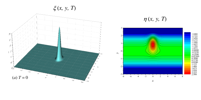
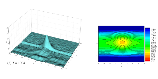
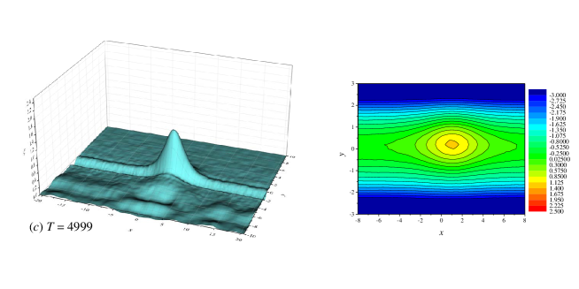
Figures 2 and 3 show the single vortex profiles $\eta(x,y,T)$ of solutions of the Gaussian and the ZK profile initial conditions with the shear flow $f_{1}=1.2$ for several time steps: $T\sim 0,1000,5000,10000$, respectively. In each case, the vortex moves to the right (positive $x$ direction) with roughly a constant speed. In the Gaussian case Fig.2, the shape is a typical oval and for later time it gradually dissipate and becomes small. On the other hand, in the ZK initial condition, the shape keeps for longer period than the Gaussian case (see Fig.3).

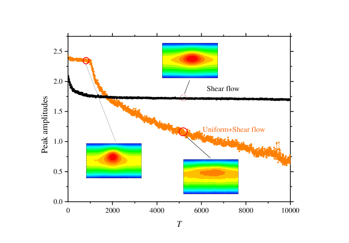
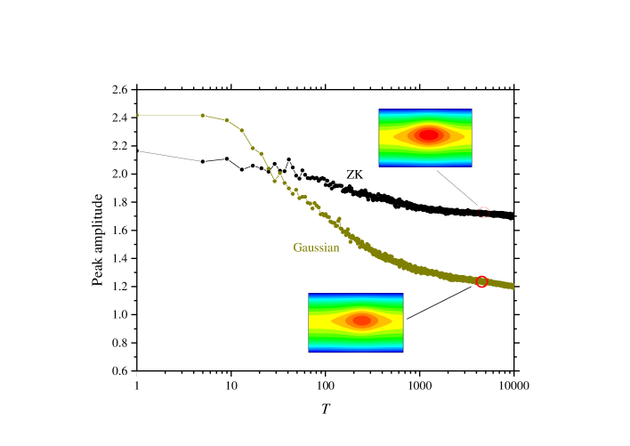
In order to see the effects of the background uniform flow, we examine evolution of the peak behavior of the solutions. Figure 4 compares peak amplitude with/without the uniform flow over the long term simulation, which shows the uniform flow destabilizes the solutions unexpectedly. Here, the initial profile is the ZK for both simulations. For $f_{0}=0.0$, after some small arrangements at the initial stage of the simulation, at $T\sim 2000$, the solution becomes more stable and this continues until the end of the simulation $T=10000$ with a very small dissipation. On the other hand, with the uniform flow $f_{0}=-1.0$, the solution keeps the shape at the beginning and then, begins to decay after $T=1000$ and slowly goes to collapse. Figure 5 shows the modulation of the peak amplitude of the vortex $\xi(x,y,T)$ for the initial conditions of the ZK and the Gaussian profile. In Williams and Yamagata (1984), the authors employed the simple cylindrical Gaussian profile for initial condition and all of their results ended in short life. Our result clearly indicates that the ZK profile has advantageous than the Gaussian. This suggests us that our solutions share some basic feature with that of the ZK equation because most of the terms in the equations are common and the WYF equation partially inherits the integrable structure of the ZK equation.

Figure 6:  $\xi(x,y,T)$ in $f_{0}=0.0$ with several $f_{1}$ in short period time evolution: $0\leq T\leq 100$. The $x$-slice solutions with $f_{1}=0.2,0.6,1.2$ are plotted. In the case $f_{1}=0.2$, the solution collapses at $T\sim 38$.

Figure 7:  $\xi(x,y,T)$ in $f_{0}=-1.0$ with several $f_{1}$ in short period time evolution: $0\leq T\leq 100$. The $x$-slice solutions with $f_{1}=0.2,0.6,1.2$ are plotted.

Figure 8:  The long-term behavior of the vortex in $f_{0}=0.0$ with $f_{1}=0.2,0.4,0.8,1.2,1.4$. The solution with $f_{1}=1.2$ is stable and has a longevity.

Figure 9:  Behaviors of the peak amplitude of the vortices in $f_{0}=0.0$ with $f_{1}=1.2,1.4,1.6,1.8$. For $f_{1}\geqq 1.4$, excited vibrations is observed but is more apparent in the case of $f_{1}=1.6,1.8$. Especially, case of $f_{1}=1.8$, the peak moves to the boundary area so we plot the value on $y\sim 1.0$.

Figure 10:  Collision of the two vortices; The profiles $\xi(x,y,T)$ in $(f_{0}.f_{1})=(0.0,1.0)$. We employ the initial condition with ZK solutions with the taller (faster) vortex $c=1.5$ and the smaller (slower) one $c=1.0$.

Figure 11:  Same as Fig.10, but here are the plots of the profiles $\eta(x,y,T)$.

Figure 12:  The long term behavior of collision of the two vortices in $f_{0}=0.0$ with $f_{1}=0.2,0.4,0.6,1.0,1.2$. The solution with $f_{1}=1.4$ rather oscillates and slightly is attenuated (similar behavior is observed in the single vortex, see Fig.8). The peaks are observed at $T\sim 15$ where the two vortices collide and merge. For solutions prior to the collisions, we plot the peak values of the larger vortex. After the collision, the solutions behave as single large vortices without large dissipation.

Figure 13:  The configurational entropy for several WYF vortices $\xi(x,y,T)$ with the various shear flows $f_{1}$. The initial condition is the ZK profile of $c=1$. We plot of the time step $T=1000,3000,5000,7000,9000$ and 10000.

Figure 14:  The configurational entropy for the two collision vortices $\xi(x,y,T)$ in $f_{0}=0.0$ with the shear flows $f_{1}=0.6,1.0$. The $f_{1}=1.0$ corresponds to Fig.10. The blue shaded areas indicate the time period where the two vortices collide.

III.3 The strength of the background flows: uniform and shear

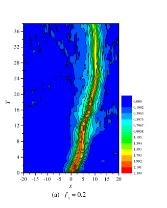
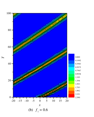
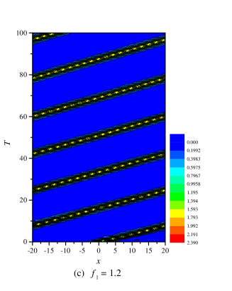
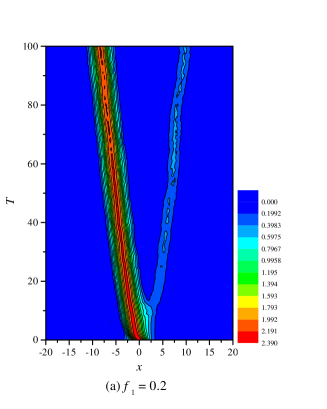
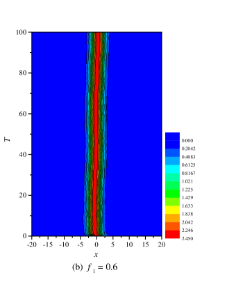
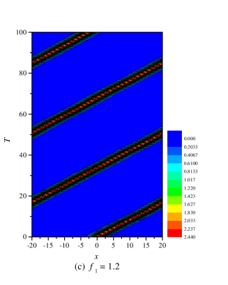
On the stability of the vortices in the WYF equation, we find the intensity of the shear flow apparently plays a dominant role. Here, we examine the time evolution of the solution with different values of strength of the shear flow. In Fig.6, we plot the time evolution of the solutions in $x$-direction at fixed $y$ value for the shear flows $f_{1}$ of the strength $0.2,0.6$ and $1.2$. The behavior of the solutions is always moderate and the vortices basically move positive $x$-direction in the effect of the shear flows. As for the speed of the vortex migration, it is higher in the strong shear flow. Then in the case of weak shear flow, $f_{1}=0.2$, the vortex becomes unstable and the life is short. The vortex tends to be swept in negative $x$ direction then genuinely the vortex moves to that direction. In the case $f_{1}=0.6$, the stability improves but still it is inclined to dissipate. We find the vortex is more likely to stay stable in the case $f_{1}=1.2$. Interestingly, a short period oscillation of the peak amplitude emerges, which we shall mention later.

Shown in Fig.7 is the cases including the uniform flow $f_{0}=-1.0$. The equation is more like the ZK equation, and consequently the solutions may look stiffer. In the weak shear flows $f_{1}=0.2$, the behavior of the solution tends to be affected by a slight modulation of the backgrounds. The solution emits a small fraction at the beginning and then moves to the left. The medium case $f_{1}=0.6$, the vortex is rather stable and seems to be balanced in position. For the stronger $f_{1}$, the vortices are more stable and they move to the positive $x$ direction. Vortex translation velocity is greater with stronger shear flow $f_{1}$ as in the cases without uniform flow.

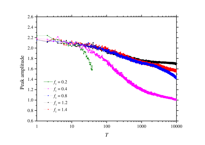
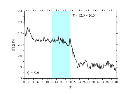
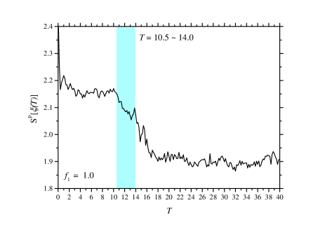
In Fig.8, we present time evolution of the peak amplitude for the several values of the shear flow $f_{1}$ without the uniform flow. As $f_{1}$ increases, the “decay rate” of the peaks gradually decreases and the solution reaches the maximum stability at $f_{1}\sim 1.2$. Above this value, the decay rate grows again as the case $f_{1}=1.4$ shows. The instability of the solutions at the larger $f_{1}$, where the decay of peak amplitude of the solution corresponds here, is indicated in Fig.9, in which we find the oscillation of the peak amplitude begins and the decay rate increases when $f_{1}\geq 1.4$. There is nothing special at $f_{1}=1.2$ shown in Fig.9 (upper left). For larger $f_{1}$, as in Figs.9, we observe the oscillating behaviors of the peak amplitude. The solution of $f_{1}=1.8$ is unstable and the peak quickly moves to one of the $y$ boundaries, for this reason the lower right panel in Fig.9 plots the peak at $y\sim 1$. These results suggest that the instability of the vortices is caused by the breakdown in the balance of the influx from the background flows and the dissipation of the energy.

We have thus confirmed that a constant shear flow with suitable value provides the longevity of vortices, and a uniform flow disturbs it.

III.4 The vector nonlinearity and vortex fusion

The stability of the vortices in the present model is due to several distinct effects: the strength of the background shear flows and the particular type of nonlinearities. In the equation (11), there are two different nonlinear terms: the KdV like term and the Jacobian term, are referred to as the scalar nonlinear term and the vector nonlinear term, respectively. Both the nonlinear terms affect with the same order of intensity, i.e., controlled by the $O(1)$ parameters $E$ and $S$.

Naive consideration from soliton theory indicates that the single vortices would collapse within a short time period when the nonlinear terms are absent due to the dispersive nature of the model, and the nonlinearity would stabilize them. For the models in two-dimensional space, however, the situation becomes considerably complicated at the collisions of multi-solitons because of their non-integrability. For example, the two solitons of the ZK equation (3) collide inelastically such that the taller soliton gets more amplitude and the smaller one becomes smaller with ripples generated Iwasaki et al. (1990).

Although the instability at the soliton collisions is expected in those two-dimensional models, we now see another kind of stability in the WYF model caused by vector nonlinearity. In Williams and Yamagata (1984), the authors extensively studied the two vortex collision process and observed that after the collision the two vortices are merged with each other. Here we reproduce the two vortex collision with the simple superposition of the two ZK initial profiles $\Phi_{c}(\tilde{r})$ of $c=1.5$ and $c=1.0$

$$\eta_{\rm init}(x,y,T=0)=\Phi_{c=1.5}(r_{1})+\Phi_{c=1}(r_{2})\,,$$

$$\hskip 56.9055ptr_{1}:=\sqrt{(x+5)^{2}+(y-1)^{2}}\,,~{}~{}r_{2}:=\sqrt{(x-5)^{2}+(y-1)^{2}}\,,$$ (25)

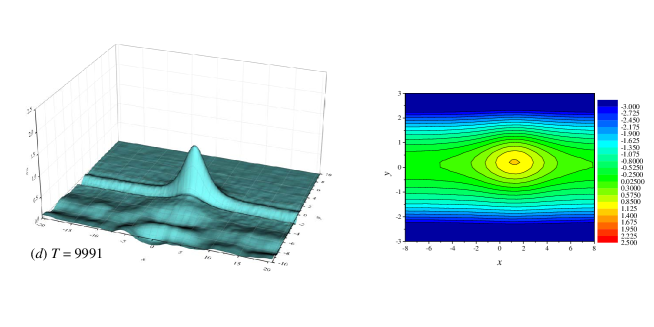
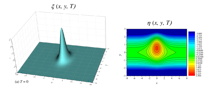
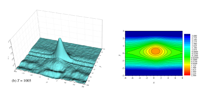
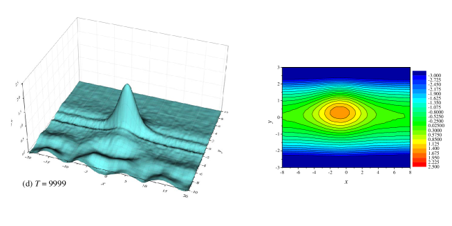
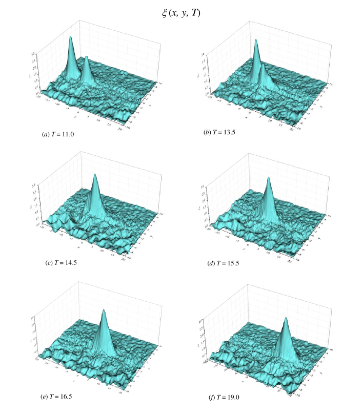
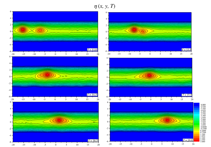
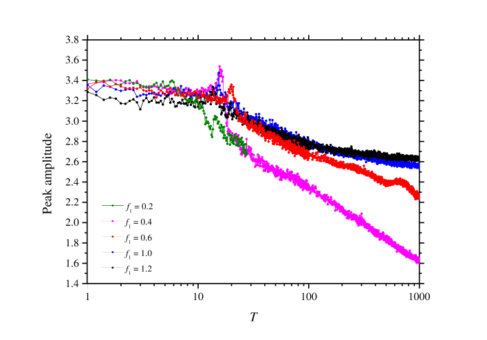
and show that the merged vortex is sufficiently stable. Fig.11 and Fig. 10 show the behavior in the collision of the profiles in contour plot and 3-dimensional plot, respectively. We find the two individual vortices on the same $y$-location with different amplitude and $x$-velocity are merged into one single vortex. The stability or longevity of the vortex after the fusion is depicted in Fig. 12 with several values of shear flow. The result shows the long-term stability of the single vortex after the fusion in the case of shear value $f_{1}=1.2$, which is consistent with the single vortex cases in the previous subsection. In fact, such a merging process has repeatedly been observed in the atmosphere of Jupiter.

III.5 Fourier analysis: the configurational entropy

Having seen the fusion phenomena of vortices in the WYF model, it is necessary to find a measure of the soliton excitation for further analysis on these non-linear systems. So far, we have mostly examined the peak amplitude of the vortices as the characteristic quantity of the soliton-like excitations. In the rest of this section, we will try to define the qualitative indicator for the transmutation of the solutions. To obtain further information on the dissipative behavior of the solutions, analysis using the Fourier transform may be efficient particularly. For this purpose, as an indicator we apply the so called configurational entropy (CE) Gleiser and Stamatopoulos (2012), which is essentially a measure of spatial complexity of solitonic objects, i.e., “shape information of a soliton”. The CE tells us many aspects of a soliton solution of a given physical system of our concern. It describes intrinsic structural change or it detects a bifurcation point of stable/unstable nature, and also it is expected to bring us an knowledge of longevity of the object Gleiser et al. (2018); Gleiser and Krackow (2019, 2020). The measure has been applied to many physical systems for the solitons in field theoretical context so far, and in this subsection, we employ it for the WYF vortices and see how the longevity is attained. Although this is an attempt to define an index of the soliton-like excitations and their lifetime at present, we hope the CE would be a promising measure for this kind of analysis.

We have studied the longevity of the WYF vortex with transition of the peak amplitude. It is worth investigating if property concerning the dissipation becomes more apparent by the use of Fourier analysis. Inspired by Shannon’s information entropy $S_{\rm Shannon}=-\sum p_{i}\log p_{i}$, where $\{p_{i}\},i=1,\cdots,N$ gives a discrete probability distribution, the CE has been introduced in the following manner. The Shannon’s entropy represents an absolute limit on the best possible lossless compression of any communication. Gleiser and his collaborators extended the notion into configurations of the field theoretical models as providing their informational content. If our solutions are described by the set of square-integrable bounded functions $f(\bm{x})\in L^{2}(\mathbb{R}^{d})$ and in terms of their Fourier transforms $F(\bm{k})$, we define the modal fraction

$$\mathfrak{f}(\bm{k})=\frac{F(\bm{k})}{\int F(\bm{k})d^{d}\bm{k}}\,.$$ (26)

The configurational entropy for the non-periodic solitonic object $S_{C}^{\textrm{NP}}$ is defined in terms of $f(\bm{k})$

$$S^{\textrm{NP}}[f]=-\int\tilde{f}(\bm{k})\log[\tilde{f}(\bm{k})]d^{d}k\,,$$ (27)

where $\tilde{f}(\bm{k})=\mathfrak{f}(\bm{k})/\mathfrak{f}(\bm{k})_{\textrm{max}}$ and $\mathfrak{f}(\bm{k})_{\textrm{max}}$ is the maximum fraction. For the periodic functions where a Fourier series is defined, $\mathfrak{f}(\bm{k})$ turns out to be $f_{n}=|A_{n}|^{2}/\sum|A_{n}|^{2}$, where $A_{n}$ is the coefficient of the $n$-th Fourier mode. In this case, the configurational entropy $S^{\textrm{P}}_{C}$ is defined as

$$S^{\textrm{P}}_{C}[f]=-\sum_{n}f_{n}\log[f_{n}]\,.$$ (28)

We expect the configurational entropy to behave that: (i) It promotes informational content of given configurations. (ii) It detects bifurcation of stable/unstable branch, where the entropy takes the maximal value. (iii) It reflects the structural change of the configuration. At the boundary of the domain, the entropy exhibits the extremum, often the minimum. (iv) It foresees the longevity of a configuration. In Gleiser and Stamatopoulos (2012), the authors gave the case of a Gaussian in $d$ dimension $f(r)=N\exp(-\alpha r^{2})$ as an example. Eq. (27) gives

$$S^{\textrm{NP}}(\alpha)=\frac{d}{2}(2\pi\alpha)^{d/2}\,.$$ (29)

For a very expanded Gaussian, $\alpha\to 0,~{}~{}S^{\textrm{NP}}\to 0$, while for a sharp peaked one $\alpha\to\infty,~{}~{}S^{\textrm{NP}}\to\infty$. $S^{\textrm{NP}}$ estimates the information content required in $k$-space to build the function $f(r)$. It is a useful estimate because it gives a good insight into the CE concerning the dissipative property of a soliton. During a time evolution of a soliton, if it dissipates with releasing some ripples the CE should decreases, while if the soliton is stable against decay the CE tends to be constant. From this point of view, we shall examine the CE of our vortex solutions.

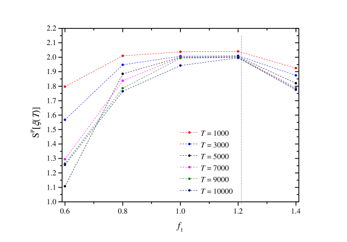
In general, the evaluation is performed for an energy density or a charge density of a given field theoretical model in the analysis of CE, from which we extract the informational contents via the energy or the topological charge structure of the model. Since our concern is how much the longevity of the soliton-like objects is achieved by both intrinsic and external effects, we evaluate the CE for the function $\xi(x,y,T)$ defined in (14) instead of the subject in the original analysis. To analyze the CE, we should evaluate the modal fraction (26) and then the non-periodic function (27), taking account of the boundary condition (18) being periodic and free-slip on $x$ and $y$ boundaries, respectively. However, it is not an easy task to implement them because of the property of this particular boundary conditions. At a glance at our numerical results, the dissipation in $y$ is relatively small and behavior of $x$ direction is almost responsible for the long-term stability so that we evaluate the CE for the $x$ section of the solutions in this paper. The Fourier series is directly obtained in the periodic boundary condition in $x$ (18), and the CE is computed using (28). Figure 13 is the CE of the WYF vortices with the ZK initial condition for varying shear flow $f_{1}$ for several time steps. The CE always takes the maximal value at $f_{1}=1.2$. As shown in Gleiser and Sowinski (2013); Gleiser and Jiang (2015), in the cases of $Q$-balls/boson stars, the maximum of the CE often detects a bifurcation point of the stable/unstable branch. The present result seems to be consistent with the previous criterion, that is, $f_{1}=1.2$ is the bifurcation point between the stable/unstable solutions. With increasing time, all the CE decay but the change is smallest at the case $f_{1}=1.2$. As a result, the solution of $f_{1}=1.2$ carries the largest informational content, which means the less dissipative, at the full-time scale.

We also examine the CE during the process of the two vortex collision in Fig.14 corresponding to Fig.12. Immediately after the collision, the CE rapidly decreases, which shows there is a release of the small fractions and slight dissipation occurs. After that, the CE quickly ceased to decrease and in fact, it stays almost constant. It means the vortex remains stable after such a collision and a merging process.

However, particularly for the tangled two-body process, the Fourier transformation in the entire two-dimension would be required for accomplishing the rigorous considerations. Such an analysis will be the next topic of this research.

IV Conclusion

We have presented two-dimensional vortex solutions in the modified Williams-Yamagata-Flierl equation (15). The equation was originally proposed in the context of geophysical fluid dynamics of the atmosphere of Jupiter and the solutions were the possible candidate for the great red spot. The model is not integrable in any sense: It has no conserved quantities and then the soliton-like stability of the solutions is not the consequence of such mathematical origin. We have found therefore the existence of solitonic objects is caused by the cooperation of several origins including external effects, i.e., the scalar/vector nonlinearities, and the shear flow. The scalar nonlinearity is equipped in Zakharov-Kuznetsov equation, which has relatively stable soliton solutions and the stability is realized by the underlying KdV dynamics. We have used the semi-analytical solutions of the Zakharov-Kusnetsov equation as an initial condition and it keeps the stability of the solution. On the other hand, the vector nonlinearity, i.e., Jacobian term has the role for the merging of two vortices upon collision, as well as the long-term stability of the single vortex of the model.

In this paper, we focused on the longevity of the vortex in terms of these effects. We carried out extremely long-term simulations and clarified how the longevity of the solutions is attained. We compared the distinct initial conditions, the ZK vortex, and the standard Gaussian function. The ZK is more stable with longevity, which means that the scalar nonlinearity has effects on the stability. Another important issue has been the background shear flows. We have performed the long-term simulation for various shear flows. The principal result of this paper is that we found the sweet spot of the value of the shear flow for stabilizing the vortex. It remains a question, however, that what is the mechanism behind the determination of this special value. We will clarify it in the subsequent paper. Another subject considered is the configurational entropy which detects the stable/unstable bifurcation point of a given solution. In terms of CE, we found that the sweet spot corresponds to the bifurcation point. It is consistent with the numerical observation. For larger $f_{1}$, apparently, the solutions become unstable.

There would be many variants to nonlinear models in higher spatial dimensions which have quasi-stable localized objects. They would have diverse types of nonlinear and external effects such as shear flows and other contents that make the solutions stable. We expect the study for such mock integrable systems will develop a fertile perspective of nonlinear dynamical systems. We will inform the results in the subsequent papers in due course.

Appendix A  The $\beta$-plane model and Williams-Yamagata-Flierl equation in the intermediate geostrophic regime

We derive the Williams-Yamagata-Flierl equation (11) for the stream function $\eta$ from the following non-dimensional “shallow water $\beta$-plane model”,

$$\hat{\varepsilon}\frac{D}{Dt}u-(1+\hat{\beta}y)v=-\frac{\partial\eta}{\partial x}\,,$$ (A.1 a)

$$\hat{\varepsilon}\frac{D}{Dt}v+(1+\hat{\beta}y)u=-\frac{\partial\eta}{\partial y}\,,$$ (A.1 b)

$$\frac{\hat{\varepsilon}}{\hat{s}}\frac{D}{Dt}\eta+\frac{\partial u}{\partial x}+\frac{\partial v}{\partial y}+\frac{\hat{\varepsilon}}{\hat{s}}\eta\left(\frac{\partial u}{\partial x}+\frac{\partial v}{\partial y}\right)=0\,,$$ (A.1 c)

where the total-derivative, or Lagrange-derivative, is defined as

$$\frac{D}{Dt}:=\frac{\partial}{\partial t}+u\frac{\partial}{\partial x}+v\frac{\partial}{\partial y}\,.$$ (A.2 )

In this model, the dimensionless parameters $\hat{\beta},\;\hat{\varepsilon}$ and $\hat{s}$ are the so-called sphericity, Rossby and stratification parameters, respectively. We apply the reductive perturbation method for the system (A.1) in terms of the sphericity parameter $\hat{\beta}\ll 1$. For this purpose, we expand the dynamical variables $u,v$ and $\eta$ in $\hat{\beta}$,

$$u=u^{(0)}+\hat{\beta}u^{(1)}+\hat{\beta}^{2}u^{(2)}+\cdots\,,$$ (A.3 a)

$$v=v^{(0)}+\hat{\beta}v^{(1)}+\hat{\beta}^{2}v^{(2)}+\cdots\,,$$ (A.3 b)

$$\eta=\eta^{(0)}+\hat{\beta}\eta^{(1)}+\hat{\beta}^{2}\eta^{(2)}+\cdots\,,$$ (A.3 c)

and substitute into (A.1). We now assume the order of the parameters as $\hat{\varepsilon}\sim\hat{\beta}^{2}$ and $\hat{s}\sim\hat{\beta}$. This parameter range is known to characterize the dynamical length scale of phenomena between the smallest scale with respect to the radius of a planet, i.e., the quasi-geostrophic (QG) scale, and the largest, i.e., the planetary-geostrophic (PG) scale, so that we refer to the scale as the intermediate-geostrophic (IG) scale. Hereafter, we introduce $O(1)$ parameters $E$ and $S$ as $\hat{\varepsilon}=E\hat{\beta}^{2}$ and $\hat{s}=S\hat{\beta}$.

First of all, we find the $O(1)$ equations in $\hat{\beta}$ of (A.1) give the relation

$$\left\{\begin{array}[]{l}\displaystyle{-v^{(0)}=-\frac{\partial\eta^{(0)}}{\partial x}}\\ \\ \displaystyle{u^{(0)}=-\frac{\partial\eta^{(0)}}{\partial y}}\end{array}\right.\ \Rightarrow\ \frac{\partial u^{(0)}}{\partial x\ }+\frac{\partial v^{(0)}}{\partial y\ }=0,$$ (A.7 )

known as the geostrophic balance. Next, the equations in $O(\hat{\beta})$ read

$$-v^{(1)}-yv^{(0)}=-\frac{\partial\eta^{(1)}}{\partial x}\,,$$ (A.8 a)

$$-u^{(1)}+yu^{(0)}=-\frac{\partial\eta^{(1)}}{\partial y}\,,$$ (A.8 b)

$$\frac{E}{S}\frac{D^{(0)}}{Dt}\eta^{(0)}+\frac{\partial u^{(1)}}{\partial x\ }+\frac{\partial v^{(1)}}{\partial y\ }+\frac{E}{S}\eta^{(0)}\left(\frac{\partial u^{(0)}}{\partial x\ }+\frac{\partial v^{(0)}}{\partial y\ }\right)=0\,,$$ (A.8 c)

where

$$\frac{D^{(0)}}{Dt}:=\frac{\partial}{\partial t}+u^{(0)}\frac{\partial}{\partial x}+v^{(0)}\frac{\partial}{\partial y}\,.$$ (A.9 )

From (A.8 a) and (A.8 b), we find

$$\frac{\partial v^{(1)}}{\partial y\ }+y\frac{\partial v^{(0)}}{\partial y\ }+v^{(0)}=\frac{\partial^{2}\eta^{(1)}}{\partial x\partial y\ }\,,$$ (A.10 )

$$\frac{\partial u^{(1)}}{\partial x\ }+y\frac{\partial u^{(0)}}{\partial x\ }\qquad=-\frac{\partial^{2}\eta^{(1)}}{\partial x\partial y\ }\,,$$ (A.11 )

which lead to

$$\frac{\partial u^{(1)}}{\partial x\ }+\frac{\partial v^{(1)}}{\partial y\ }=-v^{(0)}=-\frac{\partial\eta^{(0)}}{\partial x}.$$ (A.12 )

Substituting (A.12) into (A.8 c), a linear wave equation for $\eta^{(0)}$

$$\left(\frac{\partial}{\partial t}-\frac{S}{E}\frac{\partial}{\partial x}\right)\eta^{(0)}=0\,,$$ (A.13 )

is obtained. We therefore find that the dynamics at this order is given by a “left-moving” stationary wave packet of velocity $S/E$,

$$\eta^{(0)}=f(t+(E/S)x)\,,$$ (A.14 )

where $f$ is an arbitrary function characterizing the shape of the wave packet. We now assume that the dynamics can be decomposed into the stationary carrier wave of the form (A.14) and the other slowly moving motion. For this purpose, we introduce another time $T$ which describes the slow movement by substituting the time derivative as

$$\frac{\partial}{\partial t}\ \longrightarrow\ \frac{\partial}{\partial t}+\hat{\beta}\frac{S}{E}\frac{\partial}{\partial T}\,,$$ (A.15 )

and suppose that the zeroth order stream function $\eta^{(0)}$ is a function of $\xi:=x+(S/E)t,~{}y$ and $T$.

With these prescription, we find the equation in $O(\hat{\beta}^{2})$ are

$$E\frac{D^{(0)}}{Dt}u^{(0)}-v^{(2)}-yv^{(1)}=-\frac{\partial\eta^{(2)}}{\partial x}\,,$$ (A.16 )

$$E\frac{D^{(0)}}{Dt}v^{(0)}+u^{(2)}+yu^{(1)}=-\frac{\partial\eta^{(2)}}{\partial y}\,,$$ (A.17 )

$$\frac{E}{S}\frac{D^{(0)}}{Dt}\eta^{(1)}+\frac{\partial}{\partial T}\eta^{(0)}+\frac{\partial u^{(2)}}{\partial x}+\frac{\partial v^{(2)}}{\partial y}$$

$$+\frac{E}{S}\left\{\eta^{(0)}\left(\frac{\partial u^{(1)}}{\partial x}+\frac{\partial v^{(1)}}{\partial y}\right)+\eta^{(1)}\left(\frac{\partial u^{(0)}}{\partial x}+\frac{\partial v^{(0)}}{\partial y}\right)\right\}=0\,.$$ (A.18 )

Differentiating (A.16) and (A.17) with respect to $y$ and $x$, respectively, and eliminating $\eta^{(2)}$, reads

$$\frac{\partial u^{(2)}}{\partial x}+\frac{\partial v^{(2)}}{\partial y}=-E\left(\frac{\partial}{\partial t}\nabla^{2}\eta^{(0)}+\frac{\partial\eta^{(0)}}{\partial x}\frac{\partial}{\partial y}\nabla^{2}\eta^{(0)}-\frac{\partial\eta^{(0)}}{\partial y}\frac{\partial}{\partial x}\nabla^{2}\eta^{(0)}\right)$$

$$+y\frac{\partial\eta^{(0)}}{\partial x}-v^{(1)}$$

$$=-E\left(\nabla^{2}\frac{\partial\eta^{(0)}}{\partial x}+J(\eta^{(0)},\nabla^{2}\eta^{(0)})\right)+2y\frac{\partial\eta^{(0)}}{\partial x}-\frac{\partial\eta^{(1)}}{\partial x}\,,$$ (A.19 )

where the zeroth and the first order equations (A.7) and (A.8 a) are used, and the Laplacian is defined as

$$\nabla^{2}:=\frac{\partial^{2}}{\partial x^{2}}+\frac{\partial^{2}}{\partial y^{2}}\,.$$ (A.20 )

In the final expression, we have defined the Jacobian as

$$J(a,b) :=\frac{\partial a}{\partial x}\frac{\partial b}{\partial y}-\frac{\partial b}{\partial x}\frac{\partial a}{\partial y}\,.$$ (A.21 )

Substituting (A.19) into (A.18), we finally find the wave equation for $\eta^{(1)}$

$$\frac{E}{S}\left(\frac{\partial}{\partial t}-\frac{S}{E}\frac{\partial}{\partial x}\right)\eta^{(1)}=-\frac{\partial\eta^{(0)}}{\partial T}+S\nabla^{2}\frac{\partial\eta^{(0)}}{\partial x}+EJ(\eta^{(0)},\nabla^{2}\eta^{(0)})$$

$$-2y\frac{\partial\eta^{(0)}}{\partial x}+\frac{E}{S}\eta^{(0)}\frac{\partial\eta^{(0)}}{\partial x}\,.$$ (A.22 )

This is a wave equation for the $O(\hat{\beta})$ correction to the stream function $\eta^{(1)}$ with right-hand-side as a “forced oscillation” given by $\eta^{(0)}$. From (A.13), we find that the dispersion relation of $\eta^{(1)}$ is exactly the same as that of $\eta^{(0)}$, if we consider the homogeneous equation. Thus, there would be occurring a resonance for $\eta^{(1)}$ at the same frequency of the $O(1)$ wave $\eta^{(0)}$ concerning for the original time $t$, which strongly be a conflict with the assumption of the perturbation expansion. In order to avoid this, the right-hand-side, namely the secular term, have to vanish. We therefore find that the IG equation for $\eta^{(0)}$ with respect to the “slow time” $T$ is

$$-\frac{\partial\eta^{(0)}}{\partial T}+S\nabla^{2}\frac{\partial\eta^{(0)}}{\partial x}+EJ(\eta^{(0)},\nabla^{2}\eta^{(0)})+\frac{E}{S}\eta^{(0)}\frac{\partial\eta^{(0)}}{\partial x}-2y\frac{\partial\eta^{(0)}}{\partial x}=0\,,$$ (A.23 )

which is exactly the Williams-Yamagata-Flierl equation (11).

Appendix B  The fourth order finite difference scheme

The explicit form of the fourth order differentials for (15) are defined as follows: for the field $\xi_{i,j}\equiv\xi(x,y)$ with the grid spacing $h\equiv\Delta x,~{}\ell\equiv\Delta y$,

$$\biggl{(}\frac{\partial\xi}{\partial x}\biggr{)}_{ij}=\frac{1}{12h}\Bigl{(}-\xi_{i+2j}+8\xi_{i+1j}-8\xi_{i-1j}+\xi_{i-2j}\Bigr{)}+O(h^{5})\,,$$

$$\biggl{(}\frac{\partial^{2}\xi}{\partial x^{2}}\biggr{)}_{ij}=\frac{1}{12h^{2}}\Bigl{(}-\xi_{i+2j}+16\xi_{i+1j}-30\xi_{ij}+16\xi_{i-1j}-\xi_{i-2j}\Bigr{)}+O(h^{5})\,,$$ (B.1 )

$$\biggl{(}\frac{\partial^{3}\xi}{\partial x^{3}}\biggr{)}_{ij}=\frac{1}{2h^{3}}\Bigl{(}\xi_{i+2j}-2\xi_{i+1j}+2\xi_{i-1j}-\xi_{i-2j}\Bigr{)}+O(h^{5})\,.$$

From these, we are able to write down the mixed integral

$$\biggl{(}\frac{\partial^{3}\xi}{\partial x\partial^{2}y}\biggr{)}_{ij}=\frac{1}{144h\ell^{2}}\Bigl{[} -\Bigl{(}-\xi_{i+2j+2}+16\xi_{i+2j+1}-30\xi_{i+2j}+16\xi_{i+2j-1}-\xi_{i+2j-2}\Bigr{)}$$

$$+8\Bigl{(}-\xi_{i+1j+2}+16\xi_{i+1j+1}-30\xi_{i+1j}+16\xi_{i+1j-1}-\xi_{i+1j-2}\Bigr{)}$$

$$-8\Bigl{(}-\xi_{i-1j+2}+16\xi_{i-1j+1}-30\xi_{i-1j}+16\xi_{i-1j-1}-\xi_{i-1j-2}\Bigr{)}$$

$$+\Bigl{(}-\xi_{i-2j+2}+16\xi_{i-22j+1}-30\xi_{i-2j}+16\xi_{i-2j-1}-\xi_{i-2j-2}\Bigr{)}\Bigr{]}\,.$$ (B.2 )

For the advection term, we employ the Arakawa form which is given in the following finite difference form  Arakawa (1966)

$$J^{DD}_{ij}(\zeta,\xi):=\frac{1}{4h\ell}\Bigl{[}(\zeta_{i+1j}-\zeta_{i-1j})(\xi_{ij+1}-\xi_{ij-1})-(\zeta_{ij+1}-\zeta_{ij-1})(\xi_{i+1j}-\xi_{i-1j})\Bigr{]}\,,$$

$$J^{DC}_{ij}(\zeta,\xi):=\frac{1}{4h\ell}\Bigl{[}\zeta_{i+1j}(\xi_{i+1j+1}-\xi_{i+1j-1})-\zeta_{i-1j}(\xi_{i-1j+1}-\xi_{i-1j-1})$$

$$\hskip 113.81102pt-\zeta_{ij+1}(\xi_{i+1j+1}-\xi_{i-1j+1})+\zeta_{ij-1}(\xi_{i+1j-1}-\xi_{i-1j-1})\Bigr{]}\,,$$ (B.3 )

$$J^{CD}_{ij}(\zeta,\xi):=-J^{DC}(\xi,\zeta):=\frac{1}{4h\ell}\Bigl{[}\zeta_{i+1j+1}(\xi_{ij+1}-\xi_{i+1j})-\zeta_{i-1j-1}(\xi_{i-1j}-\xi_{ij-1})$$

$$\hskip 113.81102pt-\zeta_{i-1j+1}(\xi_{ij+1}-\xi_{i-1j})+\zeta_{i+1j-1}(\xi_{i+1j}-\xi_{ij-1})\Bigr{]}\,,$$

$$\zeta:=\nabla^{2}\xi\,,$$

and

$$J(\zeta,\xi)_{ij}:=\frac{1}{3}\Bigl{[}J^{DD}_{ij}(\zeta,\xi)+J^{DC}_{ij}(\zeta,\xi)+J^{CD}_{ij}(\zeta,\xi)\Bigr{]}\,.$$ (B.4 )

Therefore, the fourth order differential’s version can be extended via

$$J^{DD}_{ij}(\zeta,\xi):=\frac{1}{144h\ell}\Bigl{[}(-\zeta_{i+2j}+8\zeta_{i+1j}-8\zeta_{i-1j}+\zeta_{i-2j})(-\xi_{ij+2}+8\xi_{ij+1}-8\xi_{ij-1}+\xi_{ij-2})$$

$$\hskip 56.9055pt-(-\zeta_{ij+2}+8\zeta_{ij+1}-8\zeta_{ij-1}+\zeta_{ij-2})(-\xi_{i+2j}+8\xi_{i+1j}-8\xi_{i-1j}+\xi_{i-2j})\Bigr{]}\,,$$

$$J^{DC}_{ij}(\zeta,\xi):=\frac{1}{144h\ell}\Bigl{[}-\zeta_{i+2j}(-\xi_{i+2j+2}+8\xi_{i+2j+1}-8\xi_{i+2j-1}+\xi_{i+2j-2})$$

$$\hskip 113.81102pt+8\zeta_{i+1j}(-\xi_{i+1j+2}+8\xi_{i+1j+1}-8\xi_{i+1j-1}+\xi_{i+1j-2})$$

$$\hskip 113.81102pt-8\zeta_{i-1j}(-\xi_{i-1j+2}+8\xi_{i-1j+1}-8\xi_{i-1j-1}+\xi_{i-1j-2})$$

$$\hskip 113.81102pt+\zeta_{i-2j}(-\xi_{i-2j+2}+8\xi_{i-2j+1}-8\xi_{i-2j-1}+\xi_{i-2j-2})$$

$$\hskip 113.81102pt+\zeta_{ij+2}(-\xi_{i+2j+2}+8\xi_{i+1j+2}-8\xi_{i-1j+2}+\xi_{i-2j+2})$$

$$\hskip 113.81102pt-8\zeta_{ij+1}(-\xi_{i+2j+1}+8\xi_{i+1j+1}-8\xi_{i-1j+1}+\xi_{i-2j+1})$$

$$\hskip 113.81102pt+8\zeta_{ij-1}(-\xi_{i+2j-1}+8\xi_{i+1j-1}-8\xi_{i-1j-1}+\xi_{i-2j-1})$$

$$\hskip 113.81102pt-\zeta_{ij-2}(-\xi_{i+2j-2}+8\xi_{i+1j-2}-8\xi_{i-1j-2}+\xi_{i-2j-2})\,,$$ (B.5 )

$$J^{CD}_{ij}(\zeta,\xi):=-J^{DC}_{ij}(\xi,\zeta)\,.$$

References

- Ablowitz and Segur (1981) Mark J. Ablowitz and Harvey Segur, Solitons and the Inverse Scattering Transform (Society for Industrial and Applied Mathematics, 1981) https://epubs.siam.org/doi/pdf/10.1137/1.9781611970883 .
- Ablowitz and Clarkson (1991) M. A. Ablowitz and P. A. Clarkson, Solitons, Nonlinear Evolution Equations and Inverse Scattering, London Mathematical Society Lecture Note Series (Cambridge University Press, 1991).
- T.Miwa (2000) E.Date T.Miwa, M.Jimbo, Solitons: differential equations, symmetries and infinite dimensional algebras, Cambridge tracts in mathematics No. 135 (Cambridge University Press, 2000).
- Hirota (2004) Ryogo Hirota, The Direct Method in Soliton Theory, edited by Atsushi Nagai, Jon Nimmo, and Claire Gilson, Cambridge Tracts in Mathematics (Cambridge University Press, 2004).
- B.B.Kadomtsev and V.I.Petviashivilli (1970) B.B.Kadomtsev and V.I.Petviashivilli, “On the stability of solitary waves in weakly dispersive media,” Sov. Phys. Dokl 15, 539–541 (1970).
- Manakov et al. (1977) S.V. Manakov, V.E. Zakharov, L.A. Bordag, A.R. Its, and V.B. Matveev, “Two-dimensional solitons of the Kadomtsev-Petviashvili equation and their interaction,” Physics Letters A 63, 205–206 (1977).
- Davey and Stewartson (1974) A. Davey and Keith Stewartson, “On three-dimensional packets of surface waves,” Proceedings of the Royal Society of London. A. Mathematical and Physical Sciences 338, 101–110 (1974).
- Fokas and Santini (1990) A.S. Fokas and P.M. Santini, “Dromions and a boundary value problem for the davey-stewartson 1 equation,” Physica D: Nonlinear Phenomena 44, 99–130 (1990).
- Hietarinta (1990) Jarmo Hietarinta, “One-dromion solutions for genetic classes of equations,” Physics Letters A 149, 113–118 (1990).
- Nishinari and Yajima (1994) Katsuhiro Nishinari and Tetsu Yajima, “Numerical studies on stability of dromion and its collisions,” Journal of the Physical Society of Japan 63, 3538–3541 (1994), https://doi.org/10.1143/JPSJ.63.3538 .
- Ishimori (1984) Yuji Ishimori, “Multi-Vortex Solutions of a Two-Dimensional Nonlinear Wave Equation,” Progress of Theoretical Physics 72, 33–37 (1984), https://academic.oup.com/ptp/article-pdf/72/1/33/19572888/72-1-33.pdf .
- Kawahara et al. (1992) Takuji Kawahara, Keisuke Araki, and Sadayoshi Toh, “Interactions of two-dimensionally localized pulses of the regularized-long-wave equation,” Physica D: Nonlinear Phenomena 59, 79–89 (1992).
- Gao et al. (2022) Xin-Yi Gao, Yong-Jiang Guo, and Wen-Rui Shan, “Taking into consideration an extended coupled (2+1)-dimensional burgers system in oceanography, acoustics and hydrodynamics,” Chaos, Solitons and Fractals 161, 112293 (2022).
- Kaup (1981) D. J. Kaup, “The lump solutions and the bäcklund transformation for the three-dimensional three-wave resonant interaction,” Journal of Mathematical Physics 22, 1176–1181 (1981).
- Imai and Nozaki (1996) Kenji Imai and Kazuhiro Nozaki, “Lump Solutions of the Ishimori-II Equation,” Progress of Theoretical Physics 96, 521–526 (1996), https://academic.oup.com/ptp/article-pdf/96/3/521/5414710/96-3-521.pdf .
- Zhang and Ma (2017) Hai-Qiang Zhang and Wen-Xiu Ma, “Lump solutions to the 2+1-dimensional sawada-kotera equation,” Nonlinear Dynamics 87, 2305–2310 (2017).
- Zou et al. (2018) Li Zou, Zong-Bing Yu, Shou-Fu Tian, Lian-Li Feng, and Jin Li, “Lump solutions with interaction phenomena in the (2+1)-dimensional ito equation,” Modern Physics Letters B 32, 1850104 (2018), https://doi.org/10.1142/S021798491850104X .
- Anker et al. (1978) D. Anker, N. C. Freeman, and Keith Stewartson, “On the soliton solutions of the Davey-Stewartson equation for long waves,” Proceedings of the Royal Society of London. A. Mathematical and Physical Sciences 360, 529–540 (1978).
- Boiti et al. (1995) M. Boiti, L. Martina, and F. Pempinelli, “Multidimensional localized solitons,” Chaos, Solitons and Fractals 5, 2377–2417 (1995).
- Larichev and Reznik (1976) V. Larichev and G. Reznik, “Two-dimensional solitary Rossby waves,” Doklady Akademii nauk SSSR 231, 1077–1079 (1976).
- Hasegawa and Mima (1978) Akira Hasegawa and Kunioki Mima, “Pseudo-three-dimensional turbulence in magnetized nonuniform plasma,” The Physics of Fluids 21, 87–92 (1978).
- Hasegawa et al. (1979) Akira Hasegawa, Carol G. Maclennan, and Yuji Kodama, “Nonlinear behavior and turbulence spectra of drift waves and Rossby waves,” The Physics of Fluids 22, 2122–2129 (1979).
- Zakharov and Kuznetsov (1974) V. Zakharov and E A. Kuznetsov, “Three-dimensional solitons,” Soviet Physics JETP 29, 594–597 (1974).
- Petviashvili (1981) Vladimir I. Petviashvili, “Multidimensional and dissipative solitons,” Physica D: Nonlinear Phenomena 3, 329–334 (1981).
- Toh et al. (1989) Sadayoshi Toh, Hiroshi Iwasaki, and Takuji Kawahara, “Two-dimensionally localized pulses of a nonlinear equation with dissipation and dispersion,” Phys. Rev. A 40, 5472–5475 (1989).
- Melkonian and Maslowe (1989) S. Melkonian and S.A. Maslowe, “Two-dimensional amplitude evolution equations for nonlinear dispersive waves on thin films,” Physica D: Nonlinear Phenomena 34, 255–269 (1989).
- V.I.Petviashvili (1980) V.I.Petviashvili, “Red spot of Jupiter and the drift soliton in a plasma,” JETP Lett. 32, 619–621 (1980).
- Nozaki (1981) K. Nozaki, “Vortex solitons of drift waves and anomalous diffusion,” Phys. Rev. Lett. 46, 184–187 (1981).
- Xu and Shu (2005) Yan Xu and Chi-Wang Shu, “Local discontinuous galerkin methods for two classes of two-dimensional nonlinear wave equations,” Physica D: Nonlinear Phenomena 208, 21–58 (2005).
- Lannes et al. (2013) David Lannes, Felipe Linares, and Jean-Claude Saut, “The cauchy problem for the euler–poisson system and derivation of the zakharov–kuznetsov equation,” in Studies in Phase Space Analysis with Applications to PDEs, edited by Massimo Cicognani, Ferruccio Colombini, and Daniele Del Santo (Springer New York, New York, NY, 2013) pp. 181–213.
- Klein et al. (2021) Christian Klein, Svetlana Roudenko, and Nikola Stoilov, “Numerical study of Zakhavor-Kuznetsov equations in two dimensions,” Journal of Nonlinear Science 31, 1–28 (2021).
- Iwasaki et al. (1990) Hiroshi Iwasaki, Sadayoshi Toh, and Takuji Kawahara, “Cylindrical quasi-solitons of the Zakharov-Kuznetsov equation,” Physica D: Nonlinear Phenomena 43, 293–303 (1990).
- Charney and Flierl (1981) Jule G. Charney and Glenn R. Flierl, “Oceanic analogues of large-scale atmospheric motions,” Evolution of physical oceanography 504, 548 (1981).
- Bouchet and Venaille (2012) Freddy Bouchet and Antoine Venaille, “Statistical mechanics of two-dimensional and geophysical flows,” Physics reports 515, 227–295 (2012).
- Constantin (2009) Adrian Constantin, “On the relevance of soliton theory to tsunami modelling,” Wave Motion 46, 420–426 (2009).
- Constantin and Henry (2009) Adrian Constantin and David Henry, “Solitons and tsunamis,” Zeitschrift für Naturforschung A 64, 65–68 (2009).
- Constantin (2011) Adrian Constantin, Nonlinear water waves with applications to wave-current interactions and tsunamis (SIAM, 2011).
- Ibragimov et al. (2013) Ranis Ibragimov, Grace Jefferson, and John Carminati, “Invariant and approximately invariant solutions of non-linear internal gravity waves forming a column of stratified fluid affected by the earth’s rotation,” International Journal of Non-Linear Mechanics 51, 28–44 (2013).
- Ibragimov and Ibragimov (2013) Nail H. Ibragimov and Ranis N. Ibragimov, “Nonlinear whirlpools versus harmonic waves in a rotating column of stratified fluid,” Mathematical Modelling of Natural Phenomena 8, 122–131 (2013).
- Ibragimov and Lin (2017) R.N. Ibragimov and G. Lin, “Nonlinear analysis of perturbed rotating whirlpools in the ocean and atmosphere,” Mathematical Modelling of Natural Phenomena 12, 94–114 (2017).
- Nezlin and Sutyrin (1989) M.V. Nezlin and G.G. Sutyrin, “Long-lived solitary anticyclones in the planetary atmospheres and oceans, in laboratory experiments and in theory,” in Elsevier oceanography series, Vol. 50 (Elsevier, 1989) pp. 701–719.
- Nezlin et al. (1993) M. V. Nezlin, E. N. Snezhkin, A. Dobroslavsky, and A. Pletnev, Rossby vortices, spiral structures, solitons : astrophysics and plasma physics in shallow water experiments, Springer series in nonlinear dynamics (Springer-Verlag, 1993).
- Williams and Yamagata (1984) Gareth Williams and Toshio Yamagata, “Geostrophic Regimes, Intermediate Solitary Vortices and Jovian Eddies,” Journal of The Atmospheric Sciences - J ATMOS SCI 41, 453–478 (1984).
- Charney (1963) Jule G. Charney, “A note on large-scale motions in the tropics,” Journal of Atmospheric Sciences 20, 607 – 609 (1963).
- Calogero and Degasperis (1978) F. Calogero and Ao Degasperis, “Exact solution via the spectral transform of a generalization with linearly x-dependent coefficients of the modified korteweg-de-vries equation,” Lett. Nuovo Cim 22, 270–273 (1978).
- Brugarino and Pantano (1980) T. Brugarino and P. Pantano, “The integration of burgers and korteweg-de vries equations with nonuniformities,” Physics Letters A 80, 223–224 (1980).
- Joshi (1987) Nalini Joshi, “Painlevé property of general variable-coefficient versions of the korteweg-de vries and non-linear schrödinger equations,” Physics Letters A 125, 456–460 (1987).
- Hlavatỳ (1988) Ladislav Hlavatỳ, “Painlevé analysis of nonautonomous evolution equations,” Physics Letters A 128, 335–338 (1988).
- Brugarino and Greco (1991) Tommaso Brugarino and Antonio M. Greco, “Painlevé analysis and reducibility to the canonical form for the generalized kadomtsev–petviashvili equation,” Journal of mathematical physics 32, 69–71 (1991).
- Gao and Tian (2001) Yi-Tian Gao and Bo Tian, “Variable-coefficient balancing-act algorithm extended to a variable-coefficient mkp model for the rotating fluids,” International Journal of Modern Physics C 12, 1383–1389 (2001).
- Kobayashi and Toda (2005) Tadashi Kobayashi and Kouichi Toda, “A generalized kdv-family with variable coefficients in (2+ 1) dimensions,” IEICE Transactions on Fundamentals of Electronics, Communications and Computer Sciences 88, 2548–2553 (2005).
- Kobayashi and Toda (2006) Tadashi Kobayashi and Kouichi Toda, “The painlevé test and reducibility to the canonical forms for higher-dimensional soliton equations with variable-coefficients,” SIGMA. Symmetry, Integrability and Geometry: Methods and Applications 2, 063 (2006).
- Honda and Choptuik (2002) Ethan P. Honda and Matthew W. Choptuik, “Fine structure of oscillons in the spherically symmetric phi**4 Klein-Gordon model,” Phys. Rev. D 65, 084037 (2002), arXiv:hep-ph/0110065 .
- Bogolyubsky and Makhankov (1976) I. L. Bogolyubsky and V. G. Makhankov, “Lifetime of Pulsating Solitons in Some Classical Models,” Pisma Zh. Eksp. Teor. Fiz. 24, 15–18 (1976).
- Gleiser (1994) Marcelo Gleiser, “Pseudostable bubbles,” Phys. Rev. D 49, 2978–2981 (1994), arXiv:hep-ph/9308279 .
- Copeland et al. (1995) Edmund J. Copeland, M. Gleiser, and H. R. Muller, “Oscillons: Resonant configurations during bubble collapse,” Phys. Rev. D 52, 1920–1933 (1995), arXiv:hep-ph/9503217 .
- Fodor et al. (2008) Gyula Fodor, Peter Forgacs, Zalan Horvath, and Arpad Lukacs, “Small amplitude quasi-breathers and oscillons,” Phys. Rev. D 78, 025003 (2008), arXiv:0802.3525 [hep-th] .
- Fodor et al. (2009) Gyula Fodor, Peter Forgacs, Zalan Horvath, and Mark Mezei, “Oscillons in dilaton-scalar theories,” JHEP 08, 106 (2009), arXiv:0906.4160 [hep-th] .
- Gleiser and Stamatopoulos (2012) Marcelo Gleiser and Nikitas Stamatopoulos, “Entropic Measure for Localized Energy Configurations: Kinks, Bounces, and Bubbles,” Phys. Lett. B 713, 304–307 (2012), arXiv:1111.5597 [hep-th] .
- Petviashvili and Yan’kov (1982) V. I. Petviashvili and V. V. Yan’kov, “Bilayer vortices in rotating stratified fluid,” Dokl. Akad. Nauk SSSR 267, 825–828 (1982).
- Kuznetsov et al. (1986) E.A. Kuznetsov, A.M. Rubenchik, and V.E. Zakharov, “Soliton stability in plasmas and hydrodynamics,” Physics Reports 142, 103–165 (1986).
- Kaup (1993) D. J. Kaup, “Asymptotic expansions for the transmission coefficients of the so-called davey-stewartson i system,” Inverse Problems 9, 417–432 (1993).
- Zabusky (1981) Norman J. Zabusky, “Computational synergetics and mathematical innovation,” Journal of Computational Physics 43, 195–249 (1981).
- Taha and Ablowitz (1984a) Thiab R Taha and Mark I Ablowitz, “Analytical and numerical aspects of certain nonlinear evolution equations. ii. numerical, nonlinear schroedinger equation,” Journal of Computational Physics 55, 203–230 (1984a).
- Taha and Ablowitz (1984b) Thiab R. Taha and Mark I. Ablowitz, “Analytical and numerical aspects of certain nonlinear evolution equations. iii. numerical, korteweg-de vries equation,” Journal of Computational Physics 55, 231–253 (1984b).
- Li (1995) Ping-Wah Li, “On the numerical study of the kdv equation by the semi-implicit and leap-frog method,” Computer Physics Communications 88, 121–127 (1995).
- Fornberg and Whitham (1978) B. Fornberg and Gerald Beresford Whitham, “A numerical and theoretical study of certain nonlinear wave phenomena,” Philosophical Transactions of the Royal Society of London. Series A, Mathematical and Physical Sciences 289, 373–404 (1978), https://royalsocietypublishing.org/doi/pdf/10.1098/rsta.1978.0064 .
- Jain et al. (1997) P.C. Jain, Rama Shankar, and Dheeraj Bhardwaj, “Numerical solution of the korteweg-de vries (kdv) equation,” Chaos, Solitons and Fractals 8, 943–951 (1997).
- Muslu and Erbay (2003) G.M. Muslu and H.A. Erbay, “A split-step fourier method for the complex modified korteweg-de vries equation,” Computers and Mathematics with Applications 45, 503–514 (2003).
- Bona et al. (1986) Jerry L. Bona, Vassilios A. Dougalis, and Ohannes A. Karakashian, “Fully discrete galerkin methods for the korteweg-de vries equation,” Computers and Mathematics with Applications 12, 859–884 (1986).
- Smith (1985) G.D. Smith, Numerical Solution of Partial Differential Equations: Finite Difference Methods, Oxford applied mathematics and computing science series (Clarendon Press, 1985).
- Singer and Turkel (1998) I. Singer and Eli Turkel, “High order finite difference methods for the helmholtz equation,” Comput. Meth. Appl. Mech. Eng. 163 (1998).
- Hassanien et al. (2005) I.A. Hassanien, A.A. Salama, and H.A. Hosham, “Fourth-order finite difference method for solving burgers?equation,” Applied Mathematics and Computation 170, 781–800 (2005).
- Lee et al. (2014) Chaeyoung Lee, Darae Jeong, Jaemin Shin, Yibao Li, and Junseok Kim, “A fourth-order spatial accurate and practically stable compact scheme for the cahn-hilliard equation,” Physica A: Statistical Mechanics and its Applications 409, 17–28 (2014).
- Wang and Dai (2019) Xiaofeng Wang and Weizhong Dai, “A conservative fourth-order stable finite difference scheme for the generalized rosenau-kdv equation in both 1d and 2d,” Journal of Computational and Applied Mathematics 355, 310–331 (2019).
- Arakawa (1966) Akio Arakawa, “Computational design for long-term numerical integration of the equations of fluid motion: Two-dimensional incompressible flow. Part I,” Journal of Computational Physics 1, 119–143 (1966).
- Gleiser et al. (2018) Marcelo Gleiser, Michelle Stephens, and Damian Sowinski, “Configurational entropy as a lifetime predictor and pattern discriminator for oscillons,” Phys. Rev. D 97, 096007 (2018), arXiv:1803.08550 [hep-th] .
- Gleiser and Krackow (2019) Marcelo Gleiser and Max Krackow, “Resonant configurations in scalar field theories: Can some oscillons live forever?” Phys. Rev. D 100, 116005 (2019), arXiv:1906.04070 [hep-th] .
- Gleiser and Krackow (2020) Marcelo Gleiser and Max Krackow, “Configurational entropic study of the enhanced longevity in resonant oscillons,” Phys. Lett. B 805, 135450 (2020), arXiv:2003.10899 [hep-th] .
- Gleiser and Sowinski (2013) Marcelo Gleiser and Damian Sowinski, “Information-Entropic Stability Bound for Compact Objects: Application to Q-Balls and the Chandrasekhar Limit of Polytropes,” Phys. Lett. B 727, 272–275 (2013), arXiv:1307.0530 [hep-th] .
- Gleiser and Jiang (2015) Marcelo Gleiser and Nan Jiang, “Stability Bounds on Compact Astrophysical Objects from Information-Entropic Measure,” Phys. Rev. D 92, 044046 (2015), arXiv:1506.05722 [gr-qc] .