Streaming Approximation Scheme for Minimizing Total Completion Time on Parallel Machines Subject to Varying Processing Capacity

Abstract

We study the problem of minimizing total completion time on parallel machines subject to varying processing capacity. In this paper, we develop an approximation scheme for the problem under the data stream model where the input data is massive and cannot fit into memory and thus can only be scanned for a few passes. Our algorithm can compute the approximate value of the optimal total completion time in one pass and output the schedule with the approximate value in two passes.

[inst1]organization = Department of Computer Science, addressline = University of Texas Rio Grande Valley, city = Edinburg, state = TX, postcode=78539, country=USA

[inst2]organization = Department of Computer Science, addressline = College of Staten Island, CUNY, city = Staten Island, state = NY, postcode=10314, country=USA

[inst3]organization = Department of Computer Science, addressline = Purdue University Northwest, city = Hammond, state = IN, postcode=46323, country=USA

1 Introduction

In 1980, Baker and Nuttle [4] studied the problem of scheduling $n$ jobs that require a single resource whose availability varies over time. This model was motivated by the situations in which machine availability may be temporarily reduced to conserve energy or interrupted for scheduled maintenance. It also applies to situations in which processing requirements are stated in terms of man-hours and the labor availability varies over time. One example application is rotating Saturday shifts, where a company only maintains a fraction, for example 33%, of the workforce every Saturday.

In 1987, Adiri and Yehudai [1] studied the scheduling problem on single and parallel machines where the service rate of a machine remains constant while a job is being processed and may only be changed upon its completion. A simple application example is a machine tool whose performance is a function of the quality of its cutters which can be replaced only upon completion of one job.

In 2016, Hall et. al [12] proposed a new model of multitasking via shared processing which allows a team to continuously work on its main, or primary tasks while a fixed percentage of its processing capacity may be allocated to process the routinely scheduled activities such as administrative meetings, maintenance work or meal breaks. In these scenarios, a working team can be viewed as a machine with reduced capacity in some periods for processing primary jobs. A manager needs to decide how to schedule the primary jobs on these shared processing machines so as to optimize some performance criteria. In [12], the authors studied the single machine environment only. They assumed that the processing capacity allocated to all the routine jobs is a constant $e$ that is strictly less than 1.

Similar models also occur in queuing system where the number of servers can change, or where the service rate of each server can change. In [20], Teghem defined these models as the vacation models and the variable service rate models, respectively. As Doshi pointed out in [7], queuing systems where the server works on primary and secondary customers arise naturally in many computer, communication and production systems. From the point of the primary customers’ view, the server working on the secondary customers is equivalent to the server taking a vacation and not being available to the primary customers during this period.

In this paper, we extend the research on scheduling subject to varying machine processing capacity and study the problems under parallel machine environment so as to optimize some objectives. In our model, we allow different processing capacity during different periods and the change of the processing capacity is independent of the jobs. Although in some aspects the problems have been intensively studied, such as scheduling subject to unavailability constraint, this work is targeting on a more general model compared with all the above mentioned research. This generalized model apparently has a lot of applications which have been discussed in the above literature. Due to historic reasons and different application contexts, different terms have been used in literature to refer to similar concepts, including service rate [1][20], processing capacity [2][5][14], machine capacity[12], sharing ratio[12], etc. In this paper, we will adopt the term processing capacity to refer to the availability of a machine for processing the jobs.

For the proposed general model, in [9] we have studied some problems under the traditional data model where all data can be stored locally and accessed in constant time. In this paper, we will study the proposed model under the data stream environment where the input data is massive and cannot be read into memory. Specifically, we study the data stream model of our problem where the number of jobs is so big that jobs’ information cannot be stored but can only be scanned in one or more passes. This research, as in many other research areas, caters to the need for providing solutions under big data that also emerges in the area of scheduling.

As Muthukrishnan wrote in his paper [18], in the modern world, with more and more data generated, the automatic data feeds are needed for many tasks in the monitoring applications such as atmospheric, astronomical, networking, financial, sensor-related fields, etc. These tasks are time critical and thus it is important to process them in almost real time mode so as to accurately keep pace with the rate of stream updates and reflect rapidly changing trends in the data. Therefore, the researchers are facing the questions under the current and future trend of more demands of data streams processing: what can we (not) do if we are given a certain amount of resources, a data stream rate and a particular analysis task?

A natural approach to dealing with large amount of data of these time critical tasks involves approximations and developing data stream algorithms. Streaming algorithms were initially studied by Munro and Paterson in 1978 ([17]), and then by Flajolet and Martin in 1980s ([8]). The model was formally established by Alon, Matias, and Szegedy in  [3] and has received a lot of attention since then.

In this work our goal is to design streaming algorithms for our proposed problem to approximate the optimal solution in a limited number of passes over the data and using limited space. Formally, streaming algorithms are algorithms for processing the input where some or all of of the data is not available for random access but rather arrives as a sequence of items and can be examined in only a few passes (typically just one). The performance of streaming algorithms is measured by three factors: the number of passes the algorithm must run over the stream, the space needed and the update time of the algorithm.

1.1 Problem Definition

Formally our scheduling model can be defined as follows. There is a set $N=\{1,\cdots,n\}$ of $n$ jobs and $m$ parallel machines where the processing capacity of machines varies over time. Each job $j\in N$ has a processing time $p_{j}$ and can be processed by any one of the machines uninterruptedly. Associated with each machine $M_{i}$ are $l_{i}$ continuous intervals during which the processing capacity of $M_{i}$ are $\alpha_{i,1}$, $\alpha_{i,2}$, $\ldots$, $\alpha_{i,l_{i}}$, respectively, see Figure 1 for an example.

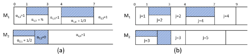
Figure 1: (a) Two machines with varying processing capacity, (b) A schedule of the 5 jobs, where $p_{1}=1$, $p_{2}=p_{3}=2$, $p_{4}=3$, $p_{5}=4$.

If the machine $M_{i}$ has full availability during an interval, we say the machine’s processing capacity is $1$ and a job, $j$, can be completed in $p_{j}$ time units; otherwise, if the machine $M_{i}$’s processing capacity is less than $1$, for example $\alpha$, then $j$ can be completed in $p_{j}/\alpha$ time units.

The objective is to minimize the total completion time of all jobs. For any schedule $S$, let $C_{j}(S)$ be the completion time of the job $j$ in $S$. If the context is clear, we use $C_{j}$ for short. The total completion time of the schedule $S$ is $\sum_{1\leq j\leq n}C_{j}$.

In this paper, we study our scheduling problem under data stream model. The goal is to design streaming algorithms to approximate the optimal solution in a limited number of passes over the data and using limited space. Using the three-field notation introduced by Graham et al. [11], our problem is denoted as $P_{m},\alpha_{i,k}\mid stream\mid\sum C_{j}$; if for all intervals, the processing capacity is greater than or equal to a constant $\alpha_{0}$, $0<\alpha_{0}\leq 1$, our problem is denoted as $P_{m},\alpha_{i,k}\geq\alpha_{0}\mid stream\mid\sum C_{j}$.

1.2 Literature Review

We first review the related work under the traditional data model. The first related work is done by Baker and Nuttle [4] in 1980. They studied the problems of sequencing $n$ jobs for processing by a single resource to minimize a function of job completion times subject to the constraint that the availability of the resource varies over time. Their work showed that a number of well-known results for classical single-machine problems can be applied with little or no modification to the corresponding variable-resource problems. Adiri and Yehudai [1] studied the problem on single and parallel machines with the restrictions such that if a job is being processed, the service rate of a machine remains constant and the service rate can be changed only when the job is completed. In 1992, Hirayama and Kijima [13] studied this problem on single machine where the machine capacity varies stochastically over time.

In 2016, Hall et. al. in [12] studied similar problems in multitasking environment, where a machine does not always have the full capacity for processing primary jobs due to previously scheduled routine jobs. In their work, they assume there is a single machine whose processing capacity is either 1 or a constant $e$ during an interval. They showed that the total completion time can be minimized by scheduling the jobs in non-decreasing order of the processing time, but it is unary NP-Hard for the objective function of total weighted completion time.

Another widely studied model is scheduling subject to machine unavailability constraint where the machine has either full capacity, or zero capacity so no jobs can be processed. Various performance criteria and machine environments have been studied under this model, see the survey papers [19] and [15] and the references therein. Among the results, for the objective of minimizing total completion time on parallel machines, the problem is NP-hard.

Other scheduling models with varying processing capacity are also studied in the literature where variation of machine availability are related with the jobs that have been scheduled. These models include scheduling with learning effects (see the survey paper [14] by Janiak et al. and the references therein), scheduling with deteriorating effects (see the paper [5] by Cheng et al.), and interdependent processing capacitys (see the paper [2] by Alidaee et al. and the references therein), etc.

In our model, there are multiple machines, the processing capacity of each machine can change between 0 and 1 from interval to interval and the capacity change can happen while a job is being processed. The goal is to find a schedule to minimize total completion time. In [9] we have showed that there is no polynomial time approximation algorithm unless $P=NP$ if the processing capacities are arbitrary for all machines. Then for the problem where the sharing ratios on some machines have a constant lower bound, we analyzed the performance of some classical scheduling algorithms and developed a polynomial time approximation scheme when the number of machines is a constant.

We now review the related work under the data stream model. Since the streaming algorithm model was formally established by Alon, Matias, and Szegedy in  [3], it has received a lot of attention. While streaming algorithms have been studied in the field of statistics, optimization, and graph algorithms (see surveys by Muthukrishnan [18] and McGregor [16]) and some research results have been obtained, very limited research on streaming algorithms ([6] [10]) has been done in the field of sequencing and scheduling so far. For the proposed model, in [10] we developed a streaming algorithm for the problem with the objective of makespan minimization.

1.3 New Contribution

In this paper, we present the first efficient streaming algorithm for the problem $P_{m},\alpha_{i,k}\geq\alpha_{0}\mid stream\mid\sum C_{j}$ . Our streaming algorithm can compute an approximation of the optimal value of the total completion time in one pass, and output a schedule that approximates the optimal schedule in two passes.

2 A PTAS for $P_{m},\alpha_{i,j}\geq\alpha_{0}\mid stream\mid\sum C_{j}$

In this section, we develop a streaming algorithm for our problem when the processing capacities on all machines have a positive constant lower bound, that is, $P_{m},\alpha_{i,k}\geq\alpha_{0}\mid stream\mid\sum C_{j}$. The algorithm is a PTAS and uses sub-linear space when $m$ is a constant.

At the conceptual level, our algorithm has the following two stages:

• Stage 1: Generate a sketch of the jobs while reading the input stream.

• Stage 2: Compute an approximation of the optimal value based on the sketch.

In the following two subsections, we will describe each stage in detail.

2.1 Stage 1: Sketch Generation from the Input Stream

In this step we read the job input stream $N=\{i:1\leq i\leq n\}$ and generate a sketch of $N$ using rounding technique. The idea of the procedure in this stage is to split the jobs into large jobs and small jobs and round the processing time of the large jobs so that the number of distinct processing times is reduced. Specifically, the sketch is a set of pairs where each pair contains a rounded processing time and the number of jobs with this rounded processing time. Let $p_{max}=\max_{j\in N}{p_{j}}$. The sketch of $N$ can be formally defined as follows:

Definition 1.

Given the error parameter $\epsilon$ and the lower bound of processing capacity of the machines $\alpha_{0}$, let $N_{L}=\{j\in N:p_{j}\geq\tfrac{\epsilon\alpha_{0}}{3n^{2}}p_{max}\}$ denote the set of large jobs. Let $\tau=\tfrac{\epsilon\alpha_{0}}{15}$, for each job $j$ of $N_{L}$, we round up its processing time such that if $p_{j}\in[(1+\tau)^{k-1},(1+\tau)^{k})$, then its rounded processing time is $rp_{k}=\left\lfloor(1+\tau)^{k}\right\rfloor$. We denote the sketch of $N$ by $N^{\prime}_{L}=\{(rp_{k},n_{k}):k_{0}\leq k\leq k_{1}\}$, where $n_{k}$ is the number of jobs whose rounded processing time is $rp_{k}$ and $k_{0}$ and $k_{1}$ are the integers such that $\tfrac{\epsilon\alpha_{0}}{3n^{2}}p_{max}\in[(1+\tau)^{k_{0}-1},(1+\tau)^{k_{0}})$ and $p_{max}\in[(1+\tau)^{k_{1}-1},(1+\tau)^{k_{1}})$ respectively.

When $n$ and $p_{max}$ are known before reading the job stream, one can generate the sketch from the job input stream with the following simple procedure: Whenever a job $j$ is read, if it is a small job, skip it and continue. Otherwise, it is a large job. Suppose that $p_{j}\in[(1+\tau)^{k-1},(1+\tau)^{k})$, we update the pair $(rp_{k},n_{k})$ by increasing $n_{k}$ by 1, where $rp_{k}=\left\lfloor(1+\tau)^{k}\right\rfloor$.

In reality, however, $n$ and $p_{max}$ may not be obtained accurately without scanning all the jobs. Meanwhile, in many practical scenarios, the estimation of $n$ and $p_{max}$ could be obtained based on priori knowledge. Specifically, an upper bound of $n$, $n^{\prime}$, could be given such that $n\leq n^{\prime}\leq c_{1}n$ for some $c_{1}\geq 1$; and a lower bound of $p_{max}$, $p^{\prime}_{max}$, could be given such that $1\leq p_{max}^{\prime}\leq p_{max}\leq c_{2}p_{max}^{\prime}$ for some $c_{2}\geq 1$. Depending on whether $n^{\prime}$ and $p^{\prime}_{max}$ are known beforehand, we have four cases: (1) both $n^{\prime}$ and $p^{\prime}_{max}$ are known; (2) only $p^{\prime}_{max}$ is known; (3) only $n^{\prime}$ is known; (4) neither $n^{\prime}$ nor $p^{\prime}_{max}$ is known.

For all four cases, we can follow the same procedure below to get the sketch of the job input stream. The main idea is as we read each job $j$, we dynamically update the maximum processing time, $p_{curMax}$, the total number of jobs, $n_{cur}$, the threshold of processing time for large jobs, $p_{minL}$, and the sketch if needed. For convenience, in the following procedure we treat $\infty$ as a number, and $1/\infty$ as $0$.

Algorithm for constructing sketch $N^{\prime}_{L}$

1. Let $\tau=\tfrac{\epsilon\alpha_{0}}{15}$

2. if $n^{\prime}$ is not given, set $n^{\prime}=\infty$

3. if $p^{\prime}_{max}$ is not given, set $p^{\prime}_{max}=1$

4. $p_{minL}=\max\{\tfrac{\epsilon\alpha_{0}}{3(n^{\prime})^{2}}p^{\prime}_{max},1\}$,

5. Initialize $p_{curMax}=0$, $n_{cur}=0$, and $N^{\prime\prime}_{L}=\emptyset$

6. Construct $N^{\prime\prime}_{L}$ while repeatedly reading next $p_{j}$

   1. $n_{cur}=n_{cur}+1$

   2. If $p_{j}>p_{curMax}$

   3. $p_{curMax}=p_{j}$

   4. if $p_{minL}<\tfrac{\epsilon\alpha_{0}}{3(n^{\prime})^{2}}\cdot p_{curMax}$, $p_{minL}=\tfrac{\epsilon\alpha_{0}}{3(n^{\prime})^{2}}\cdot p_{curMax}$

   5. If $p_{j}\geq p_{minL}$

      1. $rp=\left\lfloor(1+\tau)^{k}\right\rfloor$ where $p_{j}\in[(1+\tau)^{k-1},(1+\tau)^{k})$

      2. if there is a tuple $(rp_{k},n_{k})\in N^{\prime\prime}_{L}$ where $rp_{k}=rp$,

      3. then update $n_{k}=n_{k}+1$

      4. else

      5. $N^{\prime\prime}_{L}=N^{\prime\prime}_{L}\cup\{(rp,1)\}$

7. $p_{max}=p_{curMax}$, $n=n_{cur}$, $p_{minL}=\tfrac{\epsilon\alpha_{0}}{3n^{2}}p_{max}$

8. Let $N^{\prime}_{L}=\{(rp_{k},n_{k}):(rp_{k},n_{k})\in N^{\prime\prime}_{L},\text{ and }rp_{k}>p_{minL}\}$

While the above procedure can be used for all four cases, we need different data structures and implementations in each case to achieve time and space efficiency. For cases (1) and (2) where $p^{\prime}_{max}$ is known, since $1\leq p_{max}^{\prime}\leq p_{max}\leq c_{2}p_{max}^{\prime}$ for some constant $c_{2}$, there are at most $\log_{1+\tau}{c_{2}p^{\prime}_{max}}$ distinct rounded processing times, and thus we can use an array to store $N^{\prime\prime}_{L}$. For cases (3) and (4) where no information about $p^{\prime}_{max}$ is known, we can use a B-tree to store the elements of $N^{\prime\prime}_{L}$. Each node in the tree corresponds to an element $(rp_{k},n_{k})$ with $rp_{k}$ as the key. With $p_{curMax}$ being dynamically updated, there are at most $\log_{1+\tau}{p_{curMax}}$ distinct rounded processing times, and thus at most $\log_{1+\tau}{p_{curMax}}$ nodes in the B-tree at any time. As each job $j$ is read in, we may need to insert a new node to B-tree. If $p_{j}>p_{curMax}$, $p_{curMax}$ needs to be updated and so does $p_{minL}$, which is the threshold of processing time for large jobs. Hence the nodes with the key less than $p_{minL}$ should be removed. To minimize the worst case update time for each job, each time when a new node is inserted, we would delete the node with the smallest key if it is less than $p_{minL}$.

The following lemma gives the space and time complexity for computing sketch $N^{\prime}_{L}$ from the job input stream for all four cases.

Lemma 2.

Let $\alpha_{0}$ and $\epsilon$ be real numbers in $(0,1]$. We can compute the sketch $N^{\prime}_{L}$ of job input stream in one pass with the following performance:

1. Given both an upper bound $n^{\prime}$ for $n$ and a lower bound $p^{\prime}_{max}$ for $p_{max}$ such that $n\leq n^{\prime}\leq c_{1}n$ and $1\leq p_{max}^{\prime}\leq p_{max}\leq c_{2}p_{max}^{\prime}$ for some $c_{1}$ and $c_{2}$, then it takes $O(1)$ update time and $O(\tfrac{1}{\epsilon\alpha_{0}}\min(\log n+\log\tfrac{c_{1}c_{2}}{\epsilon\alpha_{0}},\log p_{max}+\log c_{2}))$ space to process each job from the stream.

2. Given only a lower bound $p^{\prime}_{max}$ for $p_{max}$ where $1\leq p_{max}^{\prime}\leq p_{max}\leq c_{2}p_{max}^{\prime}$, then it takes $O(1)$ update time and $O(\tfrac{1}{\epsilon\alpha_{0}}(\log p_{max}+\log c_{2}))$ space to process each job in the stream.

3. Given only an upper bound $n^{\prime}$ for $n$ such that $n\leq n^{\prime}\leq c_{1}n$, then it takes $O(\log(\tfrac{1}{\epsilon\alpha_{0}})+\min(\log(\log n+\log\tfrac{c_{1}}{\epsilon\alpha_{0}})),\log\log p_{max})$ update time, and $O(\tfrac{1}{\epsilon\alpha_{0}}\min(\log n+\log\tfrac{c_{1}}{\epsilon\alpha_{0}},\log p_{max}))$ space to process each job in the stream.

4. Given no information about $n$ and $p_{max}$, then it takes $O(\log(\tfrac{1}{\epsilon\alpha_{0}}+\log\log p_{max}))$ update time, and $O(\tfrac{1}{\epsilon\alpha_{0}}\log p_{max})$ space to process each job in the stream.

Proof.

We give the proof for four cases separately as follows:

Case 1: Both $n^{\prime}$ and $p^{\prime}_{max}$ are given such that $n\leq n^{\prime}\leq c_{1}n$, and $1\leq p_{max}^{\prime}\leq p_{max}\leq c_{2}p_{max}^{\prime}$ for some $c_{1}>1$ and $c_{2}>1$.

From the algorithm, the processing time of a large job is at most $c_{2}p^{\prime}_{max}$ and at least $p_{minL}=\max\{\tfrac{\epsilon\alpha_{0}}{3(n^{\prime})^{2}}p^{\prime}_{max},1\}$. Thus, the number of distinct processing times after rounding is at most $n^{\prime\prime}=\min(\log_{1+\tau}\tfrac{c_{2}\cdot 3(n^{\prime})^{2}}{\epsilon\alpha_{0}},\log_{1+\tau}{c_{2}p^{\prime}_{max}})$. We use an array of size $n^{\prime\prime}$ to store the elements of $N^{\prime\prime}_{L}$ and we have

$$n^{\prime\prime} =\min(\log_{1+\tau}\tfrac{c_{2}\cdot 3(n^{\prime})^{2}}{\epsilon\alpha_{0}},\log_{1+\tau}c_{2}p^{\prime}_{max})$$

$$=\log_{1+\tau}\min(\tfrac{c_{2}\cdot 3(n^{\prime})^{2}}{\epsilon\alpha_{0}},c_{2}p_{max})$$

$$\leq\log_{1+\tau}\min(\tfrac{c_{2}\cdot 3c_{1}^{2}n^{2}}{\epsilon\alpha_{0}},c_{2}p_{max})$$

$$=O(\tfrac{1}{\tau}\min(\log n+\log\tfrac{c_{1}c_{2}}{\epsilon\alpha_{0}},\log p_{max}+\log c_{2}))$$

$$=O(\tfrac{1}{\epsilon\alpha_{0}}\min(\log n+\log\tfrac{c_{1}c_{2}}{\epsilon\alpha_{0}},\log p_{max}+\log c_{2})).$$

It is easy to see that the update time for each job is $O(1)$ time.

Case 2: Only $p^{\prime}_{max}$, $p_{max}^{\prime}\leq p_{max}\leq c_{2}p_{max}^{\prime}$, is given.

From the algorithm, the processing time of a large job is between $p_{minL}=1$ and $c_{2}p^{\prime}_{max}$, thus the number of distinct processing time in $N^{\prime\prime}_{L}$ is at most $n^{\prime\prime}=\left\lfloor\log_{1+\tau}c_{2}p^{\prime}_{max}\right\rfloor\leq\left\lfloor\log_{1+\tau}c_{2}p_{max}\right\rfloor=O(\tfrac{1}{\epsilon\alpha_{0}}(\log p_{max}+\log c_{2}))$.

With the array of $n^{\prime\prime}$ elements to store the elements of $N^{\prime\prime}_{L}$, the update time for each job is $O(1)$.

Case 3: Only $n^{\prime}$, $n\leq n^{\prime}\leq c_{1}n$, is given.

We use a B-tree to store the elements of $N^{\prime\prime}_{L}$. Since $n^{\prime}$ is given, we can calculate $p_{minL}$ based on the updated $p_{curMax}$, $p_{minL}=\max\{\tfrac{\epsilon\alpha_{0}}{3(n^{\prime})^{2}}p_{curMax},1\}$. So the number of nodes in the B-tree is bounded by $\tfrac{p_{curMax}}{p_{minL}}$, which is

$$\min(\log_{1+\tau}\tfrac{3n^{\prime 2}}{\epsilon\alpha_{0}},\log_{1+\tau}p_{max})) =\log_{1+\tau}(\min(\tfrac{3n^{\prime 2}}{\epsilon\alpha_{0}},p_{max}))$$

$$\leq\log_{1+\tau}(\min(\tfrac{3c_{1}^{2}n^{2}}{\epsilon\alpha_{0}},p_{max}))$$

$$=O(\tfrac{1}{\tau}\min(\log n+\log{c_{1}\over\epsilon\alpha_{0}},\log p_{max}))$$

$$=O(\tfrac{1}{\epsilon\alpha_{0}}\min(\log n+\log\tfrac{c_{1}}{\epsilon\alpha_{0}},\log p_{max})).$$

For each large job, we need to perform at most three operations: a search operation, possibly an insertion and a deletion. The time for each operation is at most the height of the tree:

$$\log(O(\tfrac{1}{\epsilon\alpha_{0}}\min(\log n+\log\tfrac{c_{1}}{\epsilon\alpha_{0}},\log p_{max})))$$

$$= O(\log(\tfrac{1}{\epsilon\alpha_{0}})+\min(\log(\log n+\log\tfrac{c_{1}}{\epsilon\alpha_{0}}),\log\log p_{max}))$$

Case 4: No information about $p_{max}$ and $n$ is known beforehand. We still use B-tree as Case 3. However, without information of $n$, $p_{minL}$ is always 1, the total number of nodes stored in the B-tree is at most $O(\log_{1+\tau}p_{max})=O(\tfrac{1}{\epsilon\alpha_{0}}\log p_{max})$. The update time is thus $O(\log(\log_{1+\tau}p_{max}))=O(\log\tfrac{1}{\epsilon\alpha_{0}}+\log\log p_{max})$. ∎

2.2 Stage 2: Approximation Computation based on the Sketch

In this stage, we will find an approximate value of the minimum total completion time for our scheduling problem based on the sketch $N^{\prime}_{L}=\{(rp_{k},n_{k}):k_{0}\leq k\leq k_{1}\}$ that is obtained from the first stage. The idea is to assign large jobs in the sketch $N^{\prime}_{L}$ group by group in SPT order to $m$ machines where group $k$, $k_{0}\leq k\leq k_{1}$, corresponds to pair $(rp_{k},n_{k})$ in sketch $N^{\prime}_{L}$. After all groups of jobs are scheduled, we find the minimum total completion time among the remaining schedules, and return an approximate value.

To schedule each group of jobs, we perform two operations:

• Enumerate: enumerate all assignments of the jobs in the group to $m$ machines that satisfy certain property, and

• Prune: prune the schedules so that only a limited number of schedules are kept.

During the Enumerate operation, we enumerate the assignments of $n_{k}$ jobs from group $k$ to $m$ machines using $(\delta,m)$-partition as defined below.

Definition 3.

For two positive integers $b$ and $m$, and a real $\delta>0$, a $(\delta,m)$-partition of $b$ is an ordered tuple $(b_{1},b_{2},\cdots,b_{m})$ such that each $b_{i}$ is non-negative integer, $b=\sum_{1\leq i\leq m}b_{i}$, and there are at least $(m-1)$ integers $b_{i}$ is either $0$ or $\left\lfloor(1+\delta)^{q}\right\rfloor$ for some integer $q$.

For example, for $\delta=1$, to schedule a group of $b=9$ jobs to $m=3$ machines, we enumerate those assignments corresponding to $(1,3)$-partitions of $9$. From the definition, some examples of $(1,3)$-partitions of 9 are $\{2,2,5\}$, $\{0,9,0\}$, $\{0,1,8\}$. Corresponding to the partition $\{2,2,5\}$, we schedule 2 jobs on the first machine, 2 jobs on the second machine and the remaining 5 jobs on the last machine. By definition, $\{2,2,5\}$ and $\{2,5,2\}$ are two different partitions corresponding to two different schedules.

During the Prune operation, we remove some schedules so that only a limited number of schedules are kept. Let $S$ be a schedule of the jobs on $m$ machines, we use $P_{i}(S)$ to denote the total processing time of the jobs assigned to machine $M_{i}$ in $S$; and use $\sigma_{i}(S)$ to denote the total completion time of the jobs scheduled to $M_{i}$ in $S$. The schedules are pruned so that no two schedules are “similar”, where “similar” schedules are defined as follows.

Definition 4.

Two schedules $S_{1}$, $S_{2}$ are “similar” with respect to a given parameter $\delta$ if for every $1\leq i\leq m$, $P_{i}(S_{1})$ and $P_{i}(S_{2})$ are both in an interval $[(1+\delta)^{x},(1+\delta)^{x+1})$ for some integer $x$, and $\sigma_{i}(S_{1})$ and $\sigma_{i}(S_{2})$ are both in an interval $[(1+\delta)^{y},(1+\delta)^{y+1})$ for some integer $y$. We use $S_{1}\overset{\delta}{\approx}S_{2}$ to denote $S_{1}$ and $S_{2}$ are “similar” with respect to $\delta$.

Our complete algorithm for stage 2 is formally presented below in which the Enumerate and Prune operations are performed in Step (3.3.b) and (3.3.c), respectively.

Algorithm for computing the approximate value

Input: $N^{\prime}_{L}=\{(rp_{k},n_{k}):k_{0}\leq k\leq k_{1}\}$

Output: An approximate value of the minimum total completion time for jobs in $N$

Steps

1. let $\delta$ be a positive real such that $\delta<\tfrac{\epsilon\cdot\alpha_{0}}{24(k_{1}-k_{0}+1)}$

2. $U_{k_{0}-1}=\emptyset$

3. Compute $U_{k}$, $k_{0}\leq k\leq k_{1}$, which is a set of schedules of jobs from the groups $k_{0}$ to $k$

   1. let $U_{k}=\emptyset$

   2. for each $(\delta,m)$-partition of $n_{k}$

      1. for each schedule $S_{k-1}\in U_{k-1}$

      2. schedule the jobs of the group $k$ to the end of $S_{k-1}$ based

      3. on the partition and let the new schedule be $S_{k}$

      4. $U_{k}=U_{k}\cup\{S_{k}\}$

   3. prune $U_{k}$ by repeating the following until $U_{k}$ can’t be reduced

      1. if there are two schedules $S_{1}$ and $S_{2}$ in $U_{k}$ such that $S_{1}\overset{\delta}{\approx}S_{2}$

      2. $U_{k}=U_{k}\setminus\{S_{2}\}$

4. Let $S^{\prime}\in U_{k_{1}}$ be the schedule that has the minimum total completion time, $\sigma(S^{\prime})=\Sigma_{1\leq i\leq m}\sigma_{i}(S^{\prime})$.

5. return $(1+{\epsilon}/{3})(1+{\epsilon}/{15})\sigma(S^{\prime})$ as an approximate value of the minimum total completion time of the jobs in $N$.

Before we analyze the performance of the above procedure, we first consider a special case of our scheduling problem: all jobs have equal processing time and there is a single machine that has the processing capacity at least $\alpha_{0}$ at any time. Suppose that the jobs are continuously scheduled on the machine. The following lemma shows how the total completion time of these jobs changes if we shift the starting time of these jobs and/or insert additionally a small number of identical jobs at the end of these jobs.

Lemma 5.

Let $S_{x}$ be a schedule of $x$ identical jobs of processing time $p$ starting from time $t_{0}$ on a single machine whose processing capacity is at least $\alpha_{0}$ at any time. Then we have the following cases:

1. $x\cdot t_{0}+\tfrac{x(1+x)}{2}p\leq\sigma(S_{x})\leq x\cdot t_{0}+\tfrac{x(1+x)}{2\cdot\alpha_{0}}p$.

2. If we shift all jobs in $S_{x}$ so the first job starts at $(1+\delta)t_{0}$ and get a new schedule $S_{x}^{1}$, then $\sigma(S_{x}^{1})\leq(1+\tfrac{\delta}{\alpha_{0}})\sigma(S_{x})$.

3. If we add additional $\left\lfloor x\delta\right\rfloor$ identical jobs at the end of $S_{x}$ and get a new schedule $S_{x}^{2}$, then its total completion time is $\sigma(S_{x}^{2})\leq(1+\tfrac{3\delta}{\alpha_{0}})\sigma(S_{x})$.

4. Let $S_{x}^{3}$ be a schedule of $(x+\left\lfloor x\delta^{\prime}\right\rfloor)$ identical jobs of processing time $p$ starting from time $(1+\delta^{\prime\prime})t_{0}$ then $\sigma(S_{x}^{3})\leq(1+\tfrac{\delta^{\prime\prime}}{\alpha_{0}})(1+\tfrac{3\delta^{\prime}}{\alpha_{0}})\sigma(S_{x})$

Proof.

We will prove (1)-(4) one by one in order.

1. First it is easy to see that $x\cdot t_{0}+\tfrac{x(1+x)}{2}p$ is the total completion time of the jobs when the machine’s processing capacity is always 1, which is obviously a lower bound of $\sigma(S_{x})$. When the machine’s processing capacity is at least $\alpha_{0}$, then it takes at most $p/\alpha_{0}$ time to complete each job, thus the total completion time is at most $x\cdot t_{0}+\tfrac{x(1+x)}{2\cdot\alpha_{0}}p$.

2. When we shift the jobs so that the first job starts $\delta t_{0}$ later, then the completion time of each job is increased by at most $\tfrac{\delta t_{0}}{\alpha_{0}}$. Therefore,

   $$\sigma(S_{x}^{1})\leq\sigma(S_{x})+x\cdot\tfrac{\delta\cdot t_{0}}{\alpha_{0}}\leq(1+\tfrac{\delta}{\alpha_{0}})\sigma(S_{x})\enspace.$$

3. Suppose the last job in $S_{x}$ completes at time $t$. Then $t\leq t_{0}+\tfrac{xp}{\alpha_{0}}$. When we add additional $\left\lfloor x\delta\right\rfloor$ jobs starting from $t$, by (1), the total completion time of the additional jobs is at most $(x\delta\cdot t+\tfrac{x\delta(1+x\delta)}{2\cdot\alpha_{0}}p)$. Therefore,

   $$\sigma(S_{x}^{2}) \leq \sigma(S_{x})+x\delta\cdot t+\tfrac{x\delta(1+x\delta)}{2\cdot\alpha_{0}}p$$

   $$\leq \sigma(S_{x})+x\delta\cdot(t_{0}+\tfrac{xp}{\alpha_{0}})+\tfrac{\delta}{\alpha_{0}}\tfrac{x(1+x\delta)}{2}p$$

   $$\leq \sigma(S_{x})+\tfrac{\delta}{\alpha_{0}}(x\cdot t_{0}+\tfrac{x(1+x)}{2}p)+x\delta\cdot\tfrac{xp}{\alpha_{0}}$$

   $$\leq \sigma(S_{x})+\tfrac{\delta}{\alpha_{0}}\sigma(S_{x})+\tfrac{2\delta}{\alpha_{0}}\sigma(S_{x})$$

   $$\leq (1+\tfrac{3\delta}{\alpha_{0}})\sigma(S_{x})\enspace.$$

4. Follows from (2) and (3).

∎

Now we analyze the performance of our algorithm. In step 3.3.b, we only consider the schedules of the $n_{k}$ jobs corresponding to $(\delta,m)$-partitions. Let $S$ be any schedule of the jobs in sketch $N^{\prime}_{L}$, we will show that at the end of step 3.3.b there is a schedule $S_{\delta}\in U_{k}$ that is $\delta_{k}$-close to $S$. Let $n_{i,k}(S)$ be the number of jobs from group $k$ that are scheduled on machine $M_{i}$ in $S$. The $\delta_{k}$-close schedule to $S$ is defined as follows.

Definition 6.

Let $k$ be an integer such that $k_{0}\leq k\leq k_{1}$. We say a schedule $S_{\delta}$ is a $\delta_{k}$-close schedule to $S$ if for the jobs in group $k$, the following conditions hold: (1) In $S_{\delta}$, the schedule of jobs from the group $k$ form a $(\delta,m)$ partition of $n_{k}$; (2) For at least $m-1$ machines, either $n_{i,k}(S_{\delta})=0$ or $\left\lceil\log_{1+\delta}n_{i,k}(S_{\delta})\right\rceil=\left\lceil\log_{1+\delta}n_{i,k}(S)\right\rceil$.

By definition, if $S_{\delta}$ is $\delta_{k}$-close to $S$, then $n_{i,k}(S_{\delta})\leq(1+\delta)n_{i,k}(S)$ for all $i$, $1\leq i\leq m$.

The following lemma shows that there is always a schedule $S_{\delta}\in U_{k}$ at the end of step 3.3.b that is $\delta_{k}$-close to $S$.

Lemma 7.

For any schedule $S$, there exists a $\delta_{k}$-close schedule $S_{\delta}\in U_{k}$ at the end of step 3.3.b that is $\delta_{k}$-close to $S$.

Proof.

The existence of $S_{\delta}$ can be shown by construction. We initialize $S_{\delta}$ to be any schedule from $U_{k-1}$. Then we schedule the jobs from group $k$ to $M_{i}$, starting from $i=1$. Suppose there are $n_{i,k}(S)>0$ jobs scheduled on $M_{i}$ in $S$, and $(1+\delta)^{q-1}<n_{i,k}(S)\leq(1+\delta)^{q}$ for some integer $q\geq 0$, then if there are less than $\left\lfloor(1+\delta)^{q}\right\rfloor$ jobs unscheduled in this group, assign all the remaining jobs to machine $M_{i}$; otherwise, assign $\left\lfloor(1+\delta)^{q}\right\rfloor$ jobs to machine $M_{i}$ and continue to schedule the jobs of this group to the next machine.

It is easy to see that the constructed schedule of jobs from group $k$ form a $(\delta,m)$-partition that would be added to $U_{k}$ in step 3.3.b. By definition, the constructed schedule $S_{\delta}$ is a $\delta_{k}$-close schedule to $S$ . ∎

We now analyze step 3.3.c of our algorithm where “similar” schedules are pruned after a group of jobs in $N^{\prime}_{L}$ are scheduled. We will need the following notations:

$\sigma_{i,k}(S)$: the total completion time of jobs from group $k$ that are scheduled on $M_{i}$ in $S$.

$\mathcal{T}_{i,k}(S)$: the largest completion time of the jobs from group $k$ that are scheduled on $M_{i}$ in $S$.

$P_{i,k}(S)$: the total processing time of jobs from group $k$ that are scheduled to machine $M_{i}$ in $S$.

For any optimal schedule $S^{*}$ of the jobs in $N^{\prime}_{L}$, let $S_{k}^{*}$ be the partial schedule of jobs from groups $k_{0}$ to $k$ with the processing time at most $rp_{k}$ in $S^{*}$. Our next lemma shows that there is a schedule $S_{k}\in U_{k}$ that approximates the partial schedule $S_{k}^{*}$.

Lemma 8.

For any optimal schedule $S^{*}$ of the jobs in $N^{\prime}_{L}$, let $S_{k}^{*}$ be the partial schedule in $S^{*}$ of the jobs from groups $k_{0}$ to $k$. Let $\mu=k_{1}-k_{0}+1$, then after some schedules in $U_{k}$ are pruned at step (3.3.c), there exists a schedule $S_{k}\in U_{k}$ such that

1. $P_{i}(S_{k})\leq(1+\delta)^{k-k_{0}+2}P_{i}(S^{*}_{k})$ for $1\leq i\leq m$, and

2. $\sigma_{i}(S_{k})\leq(1+\delta)^{k-k_{0}+1}(1+\tfrac{2\mu\delta}{\alpha_{0}})(1+\tfrac{3\delta}{\alpha_{0}})\sigma_{i}(S^{*}_{k})$ for $1\leq i\leq m$.

Proof.

We prove by induction on $k$. First consider $k=k_{0}$. By Lemma 7, at the end of step 3.3.b there is a schedule $S^{\delta}_{k_{0}}\in U_{k_{0}}$ that is $\delta_{k_{0}}$-close to $S^{*}_{k_{0}}$, and $n_{i,k_{0}}(S^{\delta}_{k_{0}})\leq(1+\delta)n_{i,k_{0}}(S^{*}_{k_{0}})$ for all $i$, $1\leq i\leq m$ which implies $p_{i,k_{0}}(S^{\delta}_{k_{0}})\leq(1+\delta)p_{i,k_{0}}(S^{*}_{k_{0}})$. In both schedules $S^{\delta}_{k_{0}}$ and $S^{*}_{k_{0}}$, the jobs are scheduled from time 0 on each machine, by Lemma 5 Case (3), for each machine $M_{i}$, we have $\sigma_{i}(S^{\delta}_{k_{0}})\leq(1+\tfrac{3\delta}{\alpha_{0}})\sigma_{i}(S^{*}_{k_{0}})$. If $S^{\delta}_{k_{0}}$ is pruned from $U_{k_{0}}$ at step 3.3.c, then there must be a schedule $S_{k_{0}}$ such that $S_{k_{0}}\in U_{k_{0}}$ and $S^{\delta}_{k_{0}}\overset{\delta}{\approx}S_{k_{0}}$, so for each machine $M_{i}$, $1\leq i\leq m$, we have

$$P_{i}(S_{k_{0}})\leq(1+\delta)P_{i}(S^{\delta}_{k_{0}})\leq(1+\delta)^{2}P_{i}(S^{*}_{k_{0}})=(1+\delta)^{k-k_{0}+2}P_{i}(S^{*}_{k_{0}})$$

and

$$\sigma_{i}(S_{k_{0}})\leq(1+\delta)\sigma_{i}(S^{\delta}_{k_{0}})\leq(1+\delta)(1+\tfrac{3\delta}{\alpha_{0}})=(1+\delta)^{k-k_{0}+1}(1+\tfrac{3\delta}{\alpha_{0}})\sigma_{i}(S^{*}_{k_{0}}).$$

Assume the induction hypothesis holds for some $k\geq k_{0}$. So after schedules in $U_{k}$ are pruned, there is a schedule $S_{k}$ in $U_{k}$ that satisfies the inequalities (1) and (2). Now by the way that we construct schedules and by Lemma 7, in $U_{k+1}$, there must be a schedule $S_{k+1}^{\delta}\in U_{k+1}$ that is the same as $S_{k}$ for the jobs from groups $k_{0}$ to $k$, and is $\delta_{k+1}$-close to $S_{k+1}^{*}$ for the jobs of group $(k+1)$.

Then for each machine $M_{i}$ we have

$$P_{i}(S^{\delta}_{k+1}) =P_{i}(S_{k})+P_{i,k+1}(S^{\delta}_{k+1})$$

$$\leq(1+\delta)^{k-k_{0}+2}P_{i}(S^{*}_{k})+(1+\delta)P_{i,k+1}(S^{*}_{k+1})$$

$$\leq(1+\delta)^{k-k_{0}+2}P_{i}(S^{*}_{k+1})$$

And compared with $S^{*}_{k+1}$, on each machine $M_{i}$, the first job from group $(k+1)$ group in $S^{\delta}_{k+1}$ is delayed by at most $\frac{P_{i}(S_{k})-P_{i}(S^{*}_{k})}{\alpha_{0}}\leq\frac{(1+\delta)^{k-k_{0}+2}-1}{\alpha_{0}}\cdot P_{i}(S^{*}_{k})$. By Lemma 5 Case (4), for the jobs from group $k+1$ on each machine $M_{i}$, we have $\sigma_{i,k+1}(S^{\delta}_{k+1})\leq(1+\frac{(1+\delta)^{k-k_{0}+2}-1}{\alpha_{0}})(1+\tfrac{3\delta}{\alpha_{0}})\sigma_{i,k+1}(S^{*}_{k+1})$ and

$$\sigma_{i}(S^{\delta}_{k+1})$$

$$= \sigma_{i}(S_{k})+\sigma_{i,k+1}(S^{\delta}_{k+1})$$

$$\leq \sigma_{i}(S_{k})+(1+\tfrac{(1+\delta)^{k-k_{0}+2}-1}{\alpha_{0}})(1+\tfrac{3\delta}{\alpha_{0}})\cdot\sigma_{i,k+1}(S^{*}_{k+1})$$

$$\leq \sigma_{i}(S_{k})+(1+\tfrac{(1+\delta)^{\mu}-1}{\alpha_{0}})(1+\tfrac{3\delta}{\alpha_{0}})\cdot\sigma_{i,k+1}(S^{*}_{k+1})$$

$$\leq \sigma_{i}(S_{k})+(1+\tfrac{2\mu\delta}{\alpha_{0}})(1+\tfrac{3\delta}{\alpha_{0}})\cdot\sigma_{i,k+1}(S^{*}_{k+1})$$

$$\leq (1+\delta)^{k-k_{0}+1}(1+\tfrac{2\mu\delta}{\alpha_{0}})(1+\tfrac{3\delta}{\alpha_{0}})(\sigma_{i}(S^{*}_{k})+(1+\tfrac{2\mu\delta}{\alpha_{0}})(1+\tfrac{3\delta}{\alpha_{0}})\cdot\sigma_{i,k+1}(S^{*}_{k+1})$$

$$\leq (1+\delta)^{k-k_{0}+1}(1+\tfrac{2\mu\delta}{\alpha_{0}})(1+\tfrac{3\delta}{\alpha_{0}})\cdot(\sigma_{i}(S^{*}_{k})+\sigma_{i,k+1}(S^{*}_{k+1}))$$

$$\leq (1+\delta)^{k-k_{0}+1}(1+\tfrac{2\mu\delta}{\alpha_{0}})(1+\tfrac{3\delta}{\alpha_{0}})\cdot\sigma_{i}(S^{*}_{k+1})$$

Then after the “similar” schedules are pruned in our procedure, there is a schedule $S_{k+1}$ that is “similar” to $S^{\delta}_{k+1}$, so for each machines $M_{i}(1\leq i\leq m)$ we have

$$P_{i}(S_{k+1})\leq(1+\delta)P_{i}(S^{\delta}_{k+1})\leq(1+\delta)^{(k+1)-k_{0}+2}P_{i}(S^{*}_{k+1})$$

and

$$\sigma_{i}(S_{k+1})\leq(1+\delta)\sigma_{i}(S^{\delta}_{k+1})\leq(1+\delta)^{(k+1)-k_{0}+1}(1+\tfrac{2\mu\delta}{\alpha_{0}})(1+\tfrac{3\delta}{\alpha_{0}})\sigma_{i}(S^{*}_{k+1}).$$

This completes the proof. ∎

After all groups of jobs are scheduled, our algorithm finds the schedule $S^{\prime}$ that has the smallest total completion time among all generated schedules, and then returns the value $(1+{\epsilon}/{3})(1+{\epsilon}/{15})\sigma(S^{\prime})$. In the following we will show that the returned value is an approximate value of the optimal total completion time for the job set $N$.

Lemma 9.

Let $S^{*}$ be the optimal schedule for jobs in $N$, $(1+{\epsilon}/{3})(1+\epsilon/15)\sigma(S^{\prime})\leq(1+\epsilon)\sigma(S^{*})$.

Proof.

We first construct a schedule of jobs in $N$ based on the schedule $S^{\prime}$ of jobs in the sketch $N^{\prime}_{L}$ using the following two steps:

1. Replace each job in $S^{\prime}$ with the corresponding job from $N$, let the schedule be $S^{\prime\prime}$

2. Insert all small jobs from $N\setminus N_{L}$ to $M_{1}$ starting at time 0 to $S^{\prime\prime}$, and let the schedule be $S$

For each job $j$ with processing time $(1+\tau)^{k-1}\leq p_{j}<(1+\tau)^{k}$, its rounded processing time is $rp_{k}=\left\lfloor(1+\tau)^{k}\right\rfloor\geq p_{j}$, so when we replace $rp_{k}$ with $p_{j}$ to get $S^{\prime\prime}$, the completion time of each job will not increase, and thus the total completion time of jobs in $S^{\prime\prime}$ is at most that of $S^{\prime}$. That is, $\sigma(S^{\prime\prime})\leq\sigma(S^{\prime})$.

All the small jobs have processing time at most $\tfrac{\epsilon\alpha_{0}}{3n^{2}}p_{max}$, so the total length is at most $n\cdot\tfrac{\epsilon\alpha_{0}}{3n^{2}}p_{max}$. Inserting them to $M_{1}$, the completion time of the last small job in $S$ is at most $n\cdot p_{max}\tfrac{\epsilon\alpha_{0}}{3n^{2}}\cdot\tfrac{1}{\alpha_{0}}$, and the other jobs’ completion time is increased by at most $n\cdot\tfrac{\epsilon\alpha_{0}}{3n^{2}}p_{max}\cdot\tfrac{1}{\alpha_{0}}$. The total completion time of all the jobs is at most

$$\sigma(S)\leq\sigma(S^{\prime\prime})+n^{2}\cdot\tfrac{\epsilon\alpha_{0}}{3n^{2}}p_{max}\cdot\tfrac{1}{\alpha_{0}}\leq\sigma(S^{\prime\prime})+\tfrac{\epsilon}{3}\sigma(S^{\prime\prime})\leq(1+\tfrac{\epsilon}{3})\sigma(S^{\prime\prime})\leq(1+\tfrac{\epsilon}{3})\sigma(S^{\prime}).$$

By Lemma 8, there is a schedule $S_{k_{1}}\in U_{k_{1}}$ that corresponds to the schedule of the large jobs obtained from $S^{*}$. Furthermore, $\sigma(S_{{k_{1}}})\leq(1+\delta)^{\mu}(1+\tfrac{2\mu\delta}{\alpha_{0}})(1+\tfrac{3\delta}{\alpha_{0}})\sigma(S^{*}_{k_{1}})$ where $\mu=k_{1}-k_{0}+1=\log_{1+\tau}\tfrac{3n^{2}}{\epsilon\alpha_{0}}$. For schedule $S^{\prime}$, we have $\sigma(S^{\prime})\leq\sigma(S_{{k_{1}}})$. Thus,

$$\sigma(S) \leq (1+\tfrac{\epsilon}{3})\sigma(S^{\prime})$$

$$\leq (1+\tfrac{\epsilon}{3})(1+\delta)^{\mu}(1+\tfrac{2\mu\delta}{\alpha_{0}})(1+\tfrac{3\delta}{\alpha_{0}})\sigma(S^{*}_{k_{1}})$$

$$\leq (1+\tfrac{\epsilon}{3})(1+\tfrac{2\mu\delta}{\alpha_{0}})(1+\tfrac{2\mu\delta}{\alpha_{0}})(1+\tfrac{3\delta}{\alpha_{0}})\sigma(S^{*})$$

$$\leq (1+\tfrac{\epsilon}{3})(1+\tfrac{\epsilon}{12})^{2}(1+\tfrac{3\epsilon}{24\mu})\sigma(S^{*})\hskip 14.45377pt\text{plug in }\delta=\tfrac{\epsilon\alpha_{0}}{24\mu}\text{ and }\mu=\log_{1+\tau}\tfrac{3n^{2}}{\epsilon\alpha_{0}}$$

$$\leq (1+\tfrac{\epsilon}{3})(1+\tfrac{\epsilon}{12})^{2}(1+\tfrac{\epsilon}{8})\sigma(S^{*})$$

$$\leq (1+\epsilon))\cdot\sigma(S^{*})$$

∎

Lemma 10.

The Algorithm in stage 2 runs in

$$O((k_{1}-k_{0}+1)(m{\log_{1+\delta}n})^{(m-1)}({\log_{1+\delta}\tfrac{\sum p_{j}}{\alpha_{0}}})^{m}({\log_{1+\delta}(n\tfrac{\sum p_{j}}{\alpha_{0}})})^{m})$$

time using $O(({\log_{1+\delta}\tfrac{\sum p_{j}}{\alpha_{0}}})^{m}({\log_{1+\delta}(n\tfrac{\sum p_{j}}{\alpha_{0}})})^{m}))$ space.

Proof.

For each rounded processing time $rp_{k}$ and for each of $(m-1)$ machines, the number of possible jobs assigned is either $0$, or $\left\lfloor(1+\delta)^{l}\right\rfloor$, $1\leq l\leq{\log_{1+\delta}n_{k}}$, so there are $O({\log_{1+\delta}n})$ values. The remaining jobs will be assigned to the last machine. There are at most $O(m({\log_{1+\delta}n})^{m-1})$ ways to assign the jobs of a group to the $m$ machines.

For each schedule in $U_{k}$, the largest completion time is bounded by $L=\sum_{1\leq j\leq n}p_{j}/\alpha_{0}$, and its total completion time is bounded by $nL$. Since we only keep non-similar schedules, there are at most $O((\log_{1+\delta}{L})^{m}(\log_{1+\delta}{nL})^{m})$ schedules. ∎

Combining Lemma 2, Lemma 9, and Lemma 10, we get the following theorem.

Theorem 11.

Let $\alpha_{0}$ and $\epsilon$ be a real in $(0,1]$. For $P_{m},\alpha_{i,k}\geq\alpha_{0}\mid stream\mid\sum C_{j}$, there is a one-pass $(1+\epsilon)$-approximation scheme with the following time and space complexity:

1. Given both an upper bound $n^{\prime}$ for the number of jobs $n$ and a lower bound $p^{\prime}_{max}$ for the largest processing time of job $p_{max}$ such that $n\leq n^{\prime}\leq c_{1}n$ and $1\leq p_{max}^{\prime}\leq p_{max}\leq c_{2}p_{max}^{\prime}$ for some $c_{1}$ and $c_{2}$, then it takes $O(1)$ update time and $O(\tfrac{1}{\epsilon\alpha_{0}}\min(\log n+\log\tfrac{c_{1}c_{2}}{\epsilon\alpha_{0}},\log p_{max}+\log c_{2}))$ space to process each job from the stream.

2. Given only a lower bound $p^{\prime}_{max}$ for $p_{max}$ where $1\leq p_{max}^{\prime}\leq p_{max}\leq c_{2}p_{max}^{\prime}$, then it takes $O(1)$ update time and $O(\tfrac{1}{\epsilon\alpha_{0}}(\log p_{max}+\log c_{2}))$ space to process each job in the stream.

3. Given only an upper bound $n^{\prime}$ for $n$ such that $n\leq n^{\prime}\leq c_{1}n$, then it takes $O(\log(\tfrac{1}{\epsilon\alpha_{0}})+\min(\log(\log n+\log\tfrac{c_{1}}{\epsilon\alpha_{0}})),\log\log p_{max})$ update time, and $O(\tfrac{1}{\epsilon\alpha_{0}}\min(\log n+\log\tfrac{c_{1}}{\epsilon\alpha_{0}},\log p_{max}))$ space to process each job in the stream.

4. Given no information about $n$ and $p_{max}$, then it takes $O(\log(\tfrac{1}{\epsilon\alpha_{0}}+\log\log p_{max}))$ update time, and $O(\tfrac{1}{\epsilon\alpha_{0}}\log p_{max})$ space to process each job in the stream.

5. After processing the input stream, to compute the approximation value, it takes

   $$O({\epsilon\alpha_{0}}\cdot(\tfrac{360}{\epsilon^{2}\alpha_{0}^{2}}\log\tfrac{n}{\epsilon\alpha_{0}})^{3m}\cdot(m\log n)^{m-1}\cdot(\log\tfrac{\sum p_{j}}{\alpha_{0}}\cdot\log\tfrac{n\sum p_{j}}{\alpha_{0}})^{m})$$

   time using $O((\log\tfrac{n}{\epsilon\alpha_{0}})^{2m}({\log(\tfrac{\sum p_{j}}{\alpha_{0}})\log(n\tfrac{\sum p_{j}}{\alpha_{0}})})^{m})$ .

Note that our algorithm only finds an approximate value for the optimal total completion time, and it does not generate the schedule of all jobs. If the jobs can be read in a second pass, we can return a schedule of all jobs whose total completion time is at most $(1+\epsilon)\sigma(S^{*})$ where $S^{*}$ is an optimal schedule. Specifically, after the first pass, we store $n_{i,k}(S^{\prime})$, $1\leq i\leq m$, $k_{0}\leq k\leq k_{1}$, which is the number of large jobs from group $k$ that are assigned to machine $M_{i}$ in $S^{\prime}$. Based on the selected schedule $S^{\prime}$, we get $t_{i,k}$ that is the starting time for jobs from group $k$, $k_{0}\leq k\leq k_{1}$, on each machine $M_{i}$, $1\leq i\leq m$. We add group $k_{0}-1$ that includes all the small jobs and will be scheduled at the beginning on machine $M_{1}$, that is, initially $t_{1,k_{0}-1}=0$. For all $t_{1,k}$, $k_{0}\leq k\leq k_{1}$, we update it by adding $n\tfrac{\epsilon\alpha_{0}}{3n^{2}}\tfrac{p_{max}}{\alpha_{0}}$. In the second pass, for each job $j$ scanned, if it is a large job and its rounded processing time is $rp_{k}$ for some $k_{0}\leq k\leq k_{1}$, we schedule it to a machine $M_{i}$ with $n_{i,k}(S^{\prime})>0$ at $t_{i,k}$ and then update $n_{i,k}(S^{\prime})$ by decreasing by 1 and update $t_{i,k}$ accordingly; otherwise, job $j$ is a small job, and we schedule this job at $t_{1,k_{0}-1}$ on machine $M_{1}$ and update $t_{1,k_{0}-1}$ accordingly. The total space needed in the second pass is for storing $t_{i,k}$ and $n_{i,k}(S^{\prime})$ for $1\leq i\leq m$ and $k_{0}\leq k\leq k_{1}$, which is $O(m(k_{1}-k_{0}+1))=O(\tfrac{m}{\epsilon\alpha_{0}}\log\tfrac{n}{\epsilon\alpha_{0}})$.

Theorem 12.

There is a two-pass $(1+\epsilon)$-approximation streaming algorithm for $P_{m},\alpha_{i,k}\geq\alpha_{0}\mid stream\mid\sum C_{j}$. In the first pass, the approximate value can be obtained with the same metrics as Theorem 11; and in the second pass, a schedule with the approximate value can be returned with $O(1)$ processing time and $O(\tfrac{m}{\epsilon\alpha_{0}}\log\tfrac{n}{\epsilon\alpha_{0}})$ space for each job.

3 Conclusions

In this paper we studied a generalization of the classical identical parallel machine scheduling model, where the processing capacity of machines varies over time. This model is motivated by situations in which machine availability is temporarily reduced to conserve energy or interrupted for scheduled maintenance or varies over time due to the varying labor availability. The goal is to minimize the total completion time.

We studied the problem under the data stream model and presented the first streaming algorithm. Our work follows the study of streaming algorithms in the area of statistics, graph theory, etc, and leads the research direction of streaming algorithms in the area of scheduling. It is expected that more streaming algorithms based big data solutions will be developed in the future.

Our research leaves one unsolved case for the studied problems: Is there a streaming approximation scheme when one of the machines has arbitrary processing capacities? For the future work, it is also interesting to study other performance criteria under the data stream model including maximum tardiness, the number of tardy jobs and other machine environments such as uniform machines, flowshop, etc.

References

- [1] Adiri, I., and Yehudai, Z. Scheduling on machines with variable service rates. Computers & Operations Research 14, 4 (1987), 289–297.
- [2] Alidaee, B., Wang, H., Kethley, B., and Landram, F. G. A unified view of parallel machine scheduling with interdependent processing rates. Journal of Scheduling (2019), 1–17.
- [3] Alon, N., Matias, Y., and Szegedy, M. The space complexity of approximating the frequency moments. Journal of Computer and System Sciences 58, 1 (1999), 137–147.
- [4] Baker, K. R., and Nuttle, H. L. W. Sequencing independent jobs with a single resource. Naval Research Logistics Quarterly 27 (1980), 499–510.
- [5] Cheng, T. C. E., Lee, W.-C., and Wu, C.-C. Single-machine scheduling with deteriorating functions for job processing times. Applied Mathematical Modelling 34 (2010), 4171–4178.
- [6] Cormode, G., and Veselý, P. Streaming algorithms for bin packing and vector scheduling. Theory of Computing Systems 65 (2021), 916–942.
- [7] Doshi, B. T. Queueing systems with vacations—a survey. Queueing Syst. Theory Appl. 1, 1 (jan 1986), 29–66.
- [8] Flajolet, P., and Nigel Martin, G. Probabilistic counting algorithms for data base applications. Journal of Computer and System Sciences 31, 2 (1985), 182–209.
- [9] Fu, B., Huo, Y., and Zhao, H. Multitasking scheduling with shared processing, 2022. Manuscript under review.
- [10] Fu, B., Huo, Y., and Zhao, H. Streaming algorithms for multitasking scheduling with shared processing, 2022. Manuscript under revision.
- [11] Graham, R., Lawler, E., Lenstra, J., and Kan, A. Optimization and approximation in deterministic sequencing and scheduling: a survey. In Discrete Optimization II, P. Hammer, E. Johnson, and B. Korte, Eds., vol. 5 of Annals of Discrete Mathematics. Elsevier, 1979, pp. 287–326.
- [12] Hall, N. G., Leung, J. Y.-T., and lun Li, C. Multitasking via alternate and shared processing: Algorithms and complexity. Discrete Applied Mathematics 208 (2016), 41–58.
- [13] Hirayama, T., and Kijima, M. Single machine scheduling problem when the machine capacity varies stochastically. Operations Research 40 (1992), 376–383.
- [14] Janiak, A., Krysiak, T., and Trela, R. Scheduling problems with learning and ageing effects: A survey. Decision Making in Manufacturing and Services 5, 1 (Oct. 2011), 19–36.
- [15] Ma, Y., Chu, C., and Zuo, C. A survey of scheduling with deterministic machine availability constraints. Computers & Industrial Engineering 58, 2 (2010), 199–211. Scheduling in Healthcare and Industrial Systems.
- [16] Mcgregor, A. Graph stream algorithms: a survey. SIGMOD Record 43 (2014), 9–20.
- [17] Munro, J., and Paterson, M. Selection and sorting with limited storage. Theoretical Computer Science 12, 3 (1980), 315–323.
- [18] Muthukrishnan, S. Data streams: Algorithms and applications. Foundations and Trends in Theoretical Computer Science 1, 2 (aug 2005), 117–236.
- [19] Schmidt, G. Scheduling with limited machine availability1this work has been partially supported by intas grant 96-0812.1. European Journal of Operational Research 121, 1 (2000), 1–15.
- [20] Teghem, J. Control of the service process in a queueing system. European Journal of Operational Research 23, 2 (1986), 141–158.