Streaming Algorithms for
Multitasking Scheduling with Shared Processing

Abstract

In this paper, we design the first streaming algorithms for the problem of multitasking scheduling on parallel machines with shared processing. In one pass, our streaming approximation schemes can provide an approximate value of the optimal makespan. If the jobs can be read in two passes, the algorithm can find the schedule with the approximate value. This work not only provides an algorithmic big data solution for the studied problem, but also gives an insight into the design of streaming algorithms for other problems in the area of scheduling.

[inst1]organization = Department of Computer Science, addressline = University of Texas Rio Grande Valley, city = Edinburg, state = TX, postcode=78539, country=USA

[inst2]organization = Department of Computer Science, addressline = College of Staten Island, CUNY, city = Staten Island, state = NY, postcode=10314, country=USA

[inst3]organization = Department of Computer Science, addressline = Purdue University Northwest, city = Hammond, state = IN, postcode=46323, country=USA

1 Introduction

In recent years, with more and more data generated in all applications, the dimension of the computation increases rapidly. As in many other research areas, the need for providing solutions under big data also emerges in the area of scheduling. In this paper, we study the data stream model of multitasking scheduling problem. Under this data model, the input data is massive and cannot be read into memory; the goal is to design streaming algorithms to approximate the optimal solution in a few passes (typically just one) over the data and using limited space.

As Muthukrishnan addressed in his paper [24], traditionally, data are fed from the memory and one can modify the underlying data to reflect the updates; real time queries are also simple by looking up a value in the memory, as we see in banking and credit transactions; as far as complex analyses are concerned, such as trend analysis, forecasting, etc., operations are usually performed offline. However, in the modern world, with more and more data generated in the monitoring applications such as atmospheric, astronomical, networking, financial, sensor-related fields, etc., the automatic data feeds are needed for many tasks. For example, large amount of data need to be fed and processed in a short time to monitor complex correlations, track trends, support exploratory analyses and perform complex tasks such as classification, harmonic analysis etc. These tasks are time critical and thus it is important to process them in near-real time to accurately keep pace with the rate of stream updates and reflect rapidly changing trends in the data. With more data generated and more demands of data streams processing for now and in the future, the researchers are facing the questions: Given a certain amount of resources, a data stream rate and a particular analysis task, what can we (not) do?

While some methods are available for processing large amount of data of these time critical tasks, such as making things parallel, controlling data rate by sampling or shedding updates, rounding data structures to certain block boundaries, using hierarchically detailed analysis, etc., these approaches are ultimately limiting.

A natural approach to dealing with data streams involves approximations and developing algorithmic principles for data stream algorithms. Streaming algorithms were initially studied by Munro and Paterson in 1978 ([23]), and then by Flajolet and Martin in 1980s ([9]). The model was formally established by Alon, Matias, and Szegedy in  [2] and has received a lot of attention since then. Formally, streaming algorithms are algorithms for processing the input where some or all of of the data is not available for random access but rather arrives as a sequence of items and can be examined in only a few passes (typically just one). The performance of streaming algorithms is measured by three factors: the number of passes the algorithm must run over the stream, the space needed and the updating time of the algorithm.

In this paper, we study the streaming algorithms for the problem of multitasking scheduling with shared processing. Over the past couple of decades, the problem of multitasking scheduling has attracted a lot of attention in the service industries where workers frequently perform multiple tasks by switching from one task to another. For example, in health care, 21% of hospital employees spend their working time on more than one activity [25], and in consulting where workers usually engage in about 12 working spheres per day [11]. Although in the literature some research has been done on the effect of multitasking ([11], [28], [6], [26]), the study on multitasking in the area of scheduling is still very limited ([15], [16], [27], [29]).

Hall, Leung and Li ( [16] ) proposed a multitasking scheduling model that allows a team to continuously work on its main, or primary tasks while a fixed percentage of its processing capacity may be allocated to process the routinely scheduled activities as they occur. Some examples of the routinely scheduled activities are administrative meetings, maintenance work, or meal breaks. In these scenarios, some team members need to be assigned to perform these routine activities while the remaining team members still focus on the primary tasks. Since the routine activities are essential to the maintenance of the overall system in many situations, they are usually managed separately and scheduled independently of the primary jobs. When these multitasking problems are modeled in the scheduling theory, a working team is viewed as a machine which may have some periods during which routine jobs and primary jobs share the processing capacity.

In [16], it is assumed that there is only a single machine and the machine capacity allocated to routine jobs is the same for all routine jobs. In this paper, we generalize this model to parallel machine environment and allow the machine capacity allocated to routine jobs to vary from one to another. In practice, it is not uncommon that different number of team members are needed to perform different routine jobs during different time periods.

In many circumstances, it is necessary to have service continuously available for primary jobs, such as in many companies’ customer service and technical support departments, the service must be continuous for answering customers’ calls and for troubleshooting the customers’ product failures. So at least one member from the team is needed to provide these service at any time while the size of a team is typically of ten or fewer members as recommended by Dotdash Meredith Company in their management research. To model this, we allow the capacities allocated for primary jobs on some machines to have a constant lower bound.

1.1 Problem Definition

Formally, our problem can be defined as follows. We are given $m$ identical machines $\{M_{1},M_{2},\ldots,M_{m}\}$ and a set $N=\{1,\ldots,n\}$ of primary jobs that are all available for processing at time 0. Each primary job $j\in N$ has a processing time $p_{j}$ and can be processed by any one of the machines uninterruptedly. Each machine $M_{i}$ has $k_{i}$ shared processing intervals during which only a fraction of machine capacity can be allocated to these primary jobs due to the fact some capacity has been pre-allocated to routine jobs. We use “sharing ratio” to refer the fraction of the capacity allocated to the primary jobs. The total number of these intervals is $\tilde{n}=\sum_{1\leq i\leq m}k_{i}$. For simplicity, we will treat those intervals with full capacity as intervals with sharing ratio 1. Apparently, each machine $M_{i}$ has $O(k_{i})$ intervals in total. Without loss of generality, we assume that these intervals are given in sorted order, denoted as $I_{i,1}=(0,t_{i,1}]$, $I_{i,2}=(t_{i,1},t_{i,2}]$, $\ldots$, and their corresponding sharing ratios are $e_{i,1}$, $e_{i,2}$, $\ldots$, all of which are in the range of $(0,1]$, see Figure 1(a) for an illustration of machine intervals and Figure 1(b) for an illustration of a schedule of primary jobs in these intervals. For any schedule $S$, let $C_{j}(S)$ be the completion time of the primary job $j$ in $S$. If the context is clear, we use $C_{j}$ for short. The makespan of the schedule $S$ is $\max_{1\leq j\leq n}\{C_{j}\}$. The objective is to find a schedule of the primary jobs to minimize the makespan.

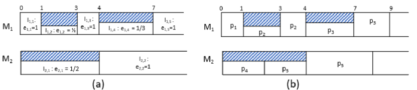
Figure 1: An example of multitasking scheduling on 2 machines with shared processing, 3 routine jobs are shown as shaded intervals. (a) The intervals and the sharing ratios; (b) A schedule of five primary jobs: $p_{1}=1$, $p_{2}=2$, $p_{3}=3$, $p_{4}=1$, $p_{5}=5$.

In this paper, we consider the above scheduling problem under the data stream model. Specifically, we study the problem that the number of primary jobs is so big that jobs’ information cannot be stored in the memory but can only be scanned in one or more passes. Extending the three-field $\alpha\mid\beta\mid\gamma$ notation introduced by Graham et al. [12], our problem is denoted as $P_{m}\mid\text{stream, share}\mid C_{max}$ if the sharing ratios are arbitrary; and if the sharing ratio is at least $e_{0}$ for the intervals on the first $m_{1}$ ($1\leq m_{1}\leq m-1$) machines but arbitrary for other $(m-m_{1})$ machines, our problem is denoted as $P_{m}\mid\text{stream, share, }e_{i,k}\geq e_{0}\text{ for }i\leq m_{1}\mid C_{max}$. The corresponding problems under the traditional data model will be denoted as $P_{m}\mid\text{share}\mid C_{max}$ and $P_{m}\mid\text{share, }e_{i,k}\geq e_{0}\text{ for }i\leq m_{1}\mid C_{max}$, respectively.

1.2 Literature Review

Various models of shared processing scheduling have been studied in the literature. In the model studied by [7], [17], [8], jobs have their own private processors and can also be processed by other processors which are shared by other jobs to reduce the job’s completion time due to processing time overlap. In the model studied by Baker and Nuttle [3], all the resources together are viewed as one machine which has varying availability over time and jobs are scheduled on this single machine with varying capacity. The authors showed that a number of well-known results for classical single-machine problems can be applied with little or no modification to the corresponding variable-resource problems. Then Hirayama and Kijima [18] studied this problem when the machine capacity varies stochastically over time. Adiri and Yehudai [1] studied the problem on single and parallel machines such that the service rate of a machine can only be changed when a job is completed.

The shared processing multitasking model studied in this paper was first proposed by Hall et. al. in [16]. In this model, machine may have reduced capacity for processing primary jobs in some periods where routine jobs are scheduled and share the processing with primary jobs. They studied this model in the single machine environment and assumed that the sharing ratio is a constant $e$ for all the shared intervals. For this model, it is easy to see that the makespan is the same for all schedules that have no unnecessary idle time. The authors in [16] showed that the total completion time can be minimized by scheduling the jobs in non-decreasing order of the processing time, but it is unary NP-Hard for the objective function of total weighted completion time. When the primary jobs have different due dates, the authors gave polynomial time algorithms for maximum lateness and the number of late jobs.

For our studied problems, if $e_{i,k}=1$ for all time intervals, that is, there are no routine jobs, the problem becomes the classical parallel machine scheduling problem $P_{m}\mid\mid C_{max}$. For this problem, Graham studied the performance of List Scheduling rule ([13]) and Longest Processing Time ([14]) rule. When the number of machines $m$ is fixed, Horowitz and Sahni [20] developed a fast approximation scheme. Later, Hochbaum and Shmoys [19] designed a approximation scheme for this problem when $m$ is arbitrary.

On the other hand, if $e_{i,k}\in\{0,1\}$ for all time intervals, i.e. at any time the machine is either processing a primary job or a routine job but not both, then our problem reduces to the problem of parallel machine scheduling with availability constraint. This problem is also NP-hard and approximation algorithms are developed in [21] and [22].

For the general problem, $P_{m}\mid share\mid C_{max}$, i.e., the sharing ratios $e_{i,k}$ are arbitrary values in $(0,1]$, Fu, et al. [10] showed that there is no approximation algorithm for the problem unless $P=NP$. Then they studied $P_{m}\mid share,e_{i,k}\geq e_{0}\mid C_{max}$ and $P_{m}\mid share,e_{i,k}\geq e_{0}\text{ for }i\leq m_{1}\mid C_{max}$, where $e_{0}$ is a constant. They analyzed the performance of some classical heuristics for the two problems. Finally, they developed an approximation scheme for the problem $P_{m}\mid share,e_{i,k}\geq e_{0}\text{ for }i\leq m_{1}\mid C_{max}$.

All the above results are for the problems under the traditional data model where all data can be stored in memory. There is no result for the studied problems under the data stream model where the input data is massive and cannot be read into memory.

While streaming algorithms have been studied in the field of statistics, optimization, and graph algorithms (see surveys by Muthukrishnan [38] and McGregor [37]) in the last twenty years, very little research is conducted in the area of scheduling and operations research in general. In [4], Beigel and Fu developed a randomized streaming approximation scheme for the bin packing problem such that it needs only constant updating time and constant space, and outputs an $(1+\epsilon)$-approximation in $(1/\epsilon)^{O(1/\epsilon)}$. In [5], Cormode and Veselý designed a streaming asymptotic $(1+\epsilon)$-approximation algorithms for bin packing and $(d+\epsilon)$-approximation for vector bin packing in $d$ dimensions. For the related vector scheduling problem, they showed how to construct an input summary in space $\widetilde{O}(d^{2}\cdot m/\epsilon^{2})$ that preserves the optimum value up to a factor of $(2-1/m+\epsilon)$, where $m$ is the number of identical machines.

1.3 New Contribution

In this work, we develop the first steaming algorithms for the generalized multitasking shared processing scheduling problems. We assume the machine information is known beforehand, but all the job information including the number of jobs and the processing times are unknown until they are read. Our streaming algorithms are approximation schemes. In one pass, for any positive constant $\epsilon$, the algorithms return a value that is at most $(1+\epsilon)$ times the optimal value of the makespan and it takes constant updating time to process each job in the stream. If the jobs can be input in two passes, the algorithms can generate the schedule with constant processing time for each job in the stream. We show that if an estimate of the maximum processing time can be obtained from priori knowledge, the approximation scheme can be implemented more efficiently. It should be noted that the approximation scheme given by Fu, et al. [10] does not work under the data stream model. So in this paper, we develop a different approximation scheme.

2 Streaming Algorithms

In this section, we will present our streaming algorithms for the multitasking scheduling problem $P_{m}\mid\text{stream, share, }\ e_{i,k}\geq e_{0}\text{ for }i\leq m_{1}\mid C_{\max}$.

We first design an approximation scheme for the studied scheduling problem under the tradition model where can be stored in the memory. We then adapt this algorithm for the following three cases, respectively: (1) the maximum job processing time, $p_{max}$, is given; (2) an estimate of $p_{max}$ is given; (3) no information about $p_{max}$ is given. In all these cases, the number of jobs is not known until all jobs are read.

2.1 An Approximation Scheme under Traditional Data Model

In [10], an approximation scheme has been developed for the studied scheduling problem under traditional data model, where the main idea is to enumerate all assignments for large jobs, prune the similar assignments, schedule the small jobs to all the obtained large job assignments, and finally pick the best schedule. This approximation scheme requires storing all the jobs information and cannot be applied to the data stream model.

So in this subsection we develop a different approximation scheme for the traditional data model but can be adapted to work under the data stream model as well. The idea of the approximation algorithm is to find the best assignment of large jobs and then generate a single schedule based on this large job assignment.

We first introduce a notation before describing our algorithm. For any time $t$, we let $A_{i}(t)$ denote the total amount of processing time of the jobs that can be processed during $(0,t]$ on machine $M_{i}$. Formally, $A_{i}(t)={t}\cdot{e_{i,1}}$ if $t\in I_{i,1}=(0,t_{i,1}]$, and $A_{i}(t)=A_{i}(t_{i,k})+{(t-t_{i,k})}\cdot{e_{i,k+1}}$ if $t\in I_{i,k+1}=(t_{i,k},t_{i,k+1}]$. By the definition of $A_{i}(t)$, if $N_{i}$ is a set of jobs assigned to machine $M_{i}$ and $\sum_{j\in N_{i}}p_{j}\leq A_{i}(t)$, then the jobs in $N_{i}$ can be completed before time $t$ on machine $M_{i}$. Let $A(t)$ be the total amount of processing time of the jobs that can be processed during $(0,t]$ on all machines, i.e., $A(t)=\sum_{i=1}^{m}A_{i}(t)$. Our algorithm is outlined as follows.

Algorithm 1

Input:

• Parameters $m$, $m_{1}$, $e_{0}$, and $\epsilon$

• The intervals $(0,t_{i,1}]$, $(t_{i,1},t_{i,2}]$, $\ldots$ on machine $M_{i}$, $1\leq i\leq m$, and their sharing ratios $e_{i,1}$, $e_{i,2}$, $\ldots$

• The number of jobs $n$, and the jobs’ processing time $p_{j}$, $1\leq j\leq n$.

Output: A schedule of $n$ jobs

Steps:

1. Identify the set of large jobs, $JS$, which is constructed below:

   1. Choose $\gamma_{0}$ and $N_{0}$ as follows:

      $$2^{\gamma_{0}} = \left\lceil\frac{m+m_{1}-1}{\tfrac{\epsilon}{2}\cdot m_{1}\cdot e_{0}}\right\rceil$$ (1)

      $$N_{0} = \left\lceil\frac{m(m+m_{1}-1)}{\tfrac{\epsilon}{4}\cdot e_{0}\cdot m_{1}}\right\rceil$$ (2)

   2. Let $p_{max}$ be the largest processing time of all the jobs. Define $\gamma_{0}+2$ continuous intervals, $IH_{-1}=(0,2^{q_{0}}]$, $IH_{0}=(2^{q_{0}},2^{q_{0}+1}]$, $\ldots$,$IH_{k}=(2^{q_{0}+k},2^{q_{0}+k+1}]$, $\ldots$ , $IH_{\gamma_{0}}=(2^{q_{0}+\gamma_{0}},2^{q_{0}+\gamma_{0}+1}]$, such that $p_{max}\in IH_{\gamma_{0}}$, i.e., $2^{q_{0}+\gamma_{0}}<p_{max}\leq 2^{q_{0}+\gamma_{0}+1}$. Correspondingly, partition the jobs in $N=\{1,2,\cdots,n\}$ into $\gamma_{0}+2$ groups, $H_{-1}$, $H_{0}$, $H_{1}$, …, $H_{\gamma_{0}}$, based on their processing time: if $p_{j}\in IH_{k}$, then add job $j$ to $H_{k}$.

   3. Let $k_{L}$, $0\leq k_{L}\leq\gamma_{0}$ be the largest index of the group that contains at least $N_{0}$ jobs; if no such group exists, i.e. all the groups have less than $N_{0}$ jobs, we let $k_{L}=-1$. Let $JS=\cup_{k>k_{L}}H_{k}$ be the set of large jobs, and the remaining jobs are considered as small jobs.

2. For each possible assignment of jobs in $JS$, find a time $t$ such that

   1. Both of the following conditions hold for $t$: (a) $A(t)\geq\sum_{i=1}^{n}p_{i}$ and (b) for $1\leq i\leq m$, $A_{i}(t)\geq P^{L}_{i}$ where $P^{L}_{i}$ is the total processing time of the large jobs assigned on $M_{i}$.

   2. At least one of (a) and (b) doesn’t hold when $t$ is replaced by ${\tfrac{t}{1+\epsilon/2}}$;

3. Among all the assignments of jobs in $JS$, we pick the one that is associated with the smallest $t$ and do the following:

   1. Assign the small jobs in any order to the machines so that at most one job finishes at or after $t$ on each machine $M_{i}$

   2. Remove the small jobs that finishes after $t$ on machine $M_{i}$, $i>m_{1}$ and schedule them to the first $m_{1}$ machines so that there are at most $\left\lceil\tfrac{m-1}{m_{1}}\right\rceil$ jobs finishing after $t$ on $M_{i}$, $i\leq m_{1}$.

4. Return the obtained schedule.

Lemma 1.

Algorithm 1 outputs a $(1+\epsilon)$-approximation for the scheduling problem $P_{m}|\text{share, }\ e_{i,k}\geq e_{0}\text{ for }i\leq m_{1}|C_{\max}$.

Proof.

First let us look at the assignment of the jobs in $JS$ that is the same as the optimal schedule. In step 2 of the algorithm, we find the time $t^{*}$ associated with this large job assignment such that both (a) and (b) hold for $t^{*}$, but either (a) or (b) doesn’t hold when $t^{*}$ is replaced by ${\tfrac{t^{*}}{1+\epsilon/2}}$, which means that $\tfrac{t^{*}}{1+\epsilon/2}<C_{max}^{*}$, i.e., $t^{*}\leq(1+\tfrac{\epsilon}{2})C_{max}^{*}$. In step 3 of the algorithm, the large job assignment associated with the smallest $t$ is selected, and we have $t\leq t^{*}\leq(1+\tfrac{\epsilon}{2})C_{max}^{*}$.

For the selected large job assignment in step 3 of the algorithm, by condition (b), all large jobs are finished before or at $t$. By condition (a), $A(t)\geq\sum_{i=1}^{n}p_{i}$, there must be at most $(m-1)$ small jobs that finish after $t$ in step 3(i), and thus in step 3(ii) we can distribute them onto the first $m_{1}$ machines so that at most $\left\lceil\tfrac{m-1}{m_{1}}\right\rceil$ small jobs on each of these machines finish after $t$. Hence, the job with the largest completion time must be on one of the first $m_{1}$ machines.

Let $j$ be the job such that $C_{j}=C_{max}$, and assume $j$ is scheduled on machine $M_{i}$, $i\leq m_{1}$. Let $U$ be the set of jobs on $M_{i}$ that finish after $t$. As the sharing ratio is at least $e_{0}$ on $M_{i}$, $C_{j}\leq t+\sum_{u\in U}\tfrac{p_{u}}{e_{0}}$. Note that all jobs in $U$ are small jobs, i.e. $p_{u}\leq 2^{q_{0}+k_{L}+1}$ for each job $u\in U$. From the analysis above, $|U|\leq\left\lceil\tfrac{m-1}{m_{1}}\right\rceil$. So,

$$C_{max}=C_{j}\leq t+\left\lceil\frac{m-1}{m_{1}}\right\rceil\cdot\frac{1}{e_{0}}\cdot 2^{q_{0}+k_{L}+1}.$$ (3)

If $k_{L}>-1$, there are at least $N_{0}$ jobs in $H_{k_{L}}$, and each of which has a processing time in the range of $(2^{q_{0}+k_{L}},2^{q_{0}+k_{L}+1}]$. Therefore, we have $C_{max}^{*}\geq\tfrac{N_{0}\cdot 2^{q_{0}+k_{L}}}{m}$, which implies $2^{q_{0}+k_{L}+1}\leq\tfrac{2mC_{max}^{*}}{N_{0}}$. Thus, we have

$$C_{max}=C_{j} \leq t+\left\lceil\frac{m-1}{m_{1}}\right\rceil\cdot\frac{1}{e_{0}}\cdot 2^{q_{0}+k_{L}+1}$$

$$\leq t+\left\lceil\frac{m-1}{m_{1}}\right\rceil\cdot\frac{1}{e_{0}}\cdot\frac{2mC_{max}^{*}}{N_{0}}$$

$$\leq t+\frac{m+m_{1}-1}{m_{1}}\cdot\frac{1}{e_{0}}\cdot\frac{2mC_{max}^{*}}{N_{0}}$$

$$\leq \left(1+\frac{\epsilon}{2}\right)C_{max}^{*}+\frac{m+m_{1}-1}{m_{1}}\cdot\frac{1}{e_{0}}\cdot\frac{2mC_{max}^{*}}{N_{0}}\text{ \hskip 7.22743pt by Equation }(\ref{select-N0-ineqn})$$

$$\leq (1+\epsilon)C_{max}^{*}\enspace.$$

Otherwise, $k_{L}=-1$, using $2^{q_{0}+\gamma_{0}}<p_{max}\leq 2^{q_{0}+\gamma_{0}+1}$, we have $2^{q_{0}+k_{L}+1}=2^{q_{0}}\leq\tfrac{p_{max}}{2^{\gamma_{0}}}\leq\tfrac{C_{max}^{*}}{2^{\gamma_{0}}}$. Therefore, we can get

$$C_{max}=C_{j} \leq t+\left\lceil\frac{m-1}{m_{1}}\right\rceil\cdot\frac{1}{e_{0}}\cdot 2^{q_{0}+k_{L}+1}$$

$$= t+\left\lceil\frac{m-1}{m_{1}}\right\rceil\cdot\frac{1}{e_{0}}\cdot 2^{q_{0}}$$

$$\leq t+\left\lceil\frac{m-1}{m_{1}}\right\rceil\cdot\frac{1}{e_{0}}\cdot\frac{C_{max}^{*}}{2^{\gamma_{0}}}$$

$$\leq t+\frac{m+m_{1}-1}{m_{1}}\cdot\frac{1}{e_{0}}\cdot\frac{C_{max}^{*}}{2^{\gamma_{0}}}$$

$$\leq \left(1+\frac{\epsilon}{2}\right)C_{max}^{*}+\frac{m+m_{1}-1}{m_{1}}\cdot\frac{1}{e_{0}}\cdot\frac{C_{max}^{*}}{2^{\gamma_{0}}}\text{ \hskip 7.22743pt by Equation }(\ref{select-gamma0-ineqn})$$

$$\leq (1+\epsilon)C_{max}^{*}\enspace.$$

So in both cases, we have $C_{max}\leq(1+\epsilon)C_{max}^{*}$. ∎

Now we analyze the running time of Algorithm 1. Let

$$t_{1}(m,m_{1},\tilde{n},\epsilon,e_{0}))=\left(m^{O(\tfrac{m^{2}}{\epsilon e_{0}m_{1}}\log\tfrac{m}{\epsilon e_{0}m_{1}})}\left(\log(\tfrac{1}{\epsilon}\log\tfrac{m}{e_{0}})\cdot\sum_{1\leq i\leq m}\log k_{i}\right)\right)\enspace,$$ (4)

then we have the following lemma for the running time of Algorithm 1.

Lemma 2.

Let $\epsilon$ be a real number in $(0,1)$, Algorithm 1 runs in time

$$O\left(n+\tilde{n}+t_{1}(m,m_{1},\tilde{n},\epsilon,e_{0}))\right),$$

which is linear $O(n+\tilde{n})$ when $m$ is constant.

Proof.

In Step 1, we find the set of large jobs $JS$ which can be done in $O(n)$ time. The number of jobs in $JS$ is at most $N_{0}(\gamma_{0}+1)$.

In step 2, we consider all possible assignments of jobs in $JS$, and there are $O(m^{O(N_{0}\gamma_{0})})$ of them. By Equation (2), we have $N_{0}=O\left(\tfrac{m(m+m_{1}-1)}{\epsilon e_{0}\cdot m_{1}}\right)=O\left(\tfrac{m^{2}}{\epsilon e_{0}\cdot m_{1}}\right)$. By Equation  (1), we have $\gamma_{0}=O\left(\log{\tfrac{m+m_{1}-1}{\epsilon e_{0}\cdot m_{1}}}\right)=O\left(\log{\tfrac{m}{\epsilon e_{0}\cdot m_{1}}}\right).$

Let $P=\sum_{i=1}^{n}p_{i}$, then the time $t$ associated with each assignment of jobs in $JS$ is between the lower bound $LB=P/m$ and the upper bound $UB=\tfrac{P}{e_{0}}=LB\cdot\tfrac{m}{e_{0}}$. It takes $O(\log(UB-LB))$ time to search the exact smallest $t$ such that both (a) and (b) hold. To speed up the algorithm, instead of searching the exact smallest $t$, we search $t$ with a $(1+\epsilon/2)$-approximation in step 2(ii). Specifically, we only need to consider those time points whose values are $LB\times(1+\tfrac{\epsilon}{2})^{x}$, where $0\leq x\leq\log_{1+\epsilon/2}\tfrac{UB}{LB}=O\left(\tfrac{1}{\epsilon}\log\tfrac{m}{e_{0}}\right)$. In this way, we can use binary search to find the corresponding $x$ in $O\left(\log(\tfrac{1}{\epsilon}\log\tfrac{m}{e_{0}})\right)$ iterations.

In each iteration of binary search, for the specific $t=LB\cdot(1+\tfrac{\epsilon}{2})^{x}$, we need to calculate $A_{i}(t)$, $1\leq i\leq m$, which is the total amount of jobs that can be processed by $t$ on machine $M_{i}$. To do so, we use binary search to find the interval $(t_{i,k-1},t_{i,{k}}]$ such that $t\in(t_{i,k-1},t_{i,{k}}]$ in $O(\log k_{i})$ time, then compute $A_{i}(t)=A_{i}(t_{i,k-1})+(t-t_{i,k-1})e_{i,k}$, which can be done in constant time if $A_{i}(t_{i,k})$ is known; indeed, we can pre-calculated $A_{i}(t_{i,k})$ for all $i$ and $t_{i,k}$ in $O(\tilde{n})$ time. Once $A_{i}(t)$ is calculated for all $i$, $1\leq i\leq m$, we have $A(t)=\sum A_{i}(t)$. In total, it takes $O(\sum_{i=1}^{m}\log k_{i})$ time to calculate $A_{i}(t)$ and $A(t)$, and check conditions (a) and (b) for $t$. With the same running time, one can calculate $A_{i}({\tfrac{t}{1+\epsilon/2}})$ and check conditions (a) and (b) for ${\tfrac{t}{1+\epsilon/2}}$. Therefore, the time of finding $t$ associated with a specific large job assignment is $\left(\log(\tfrac{1}{\epsilon}\log\tfrac{m}{e_{0}})\cdot\sum_{1\leq i\leq m}\log k_{i}\right)$. The total time for all assignments would be $t_{1}(m,m_{1},\tilde{n},\epsilon,e_{0})$, which is given by Equation (4).

In step 3, we select the assignment associated with the smallest $t$ and schedule the small jobs based on this assignment. This can be done in time $O(n+\tilde{n})$.

Adding the time in all steps, we get the total time as stated in the lemma. ∎

By Lemmas 1 and  2, we have the following theorem.

Theorem 3.

Let $\epsilon$ be a real number in $(0,1)$, and $m$ be a constant. Then there is a $(1+\epsilon)$-approximation scheme for $P_{m}|\text{ share}\ e_{i,k}\geq e_{0}\text{ for }i\leq m_{1}|C_{\max}$ in time $O(n+\tilde{n})$.

Now in the following we will adapt Algorithm 1 so it works under the streaming model where the processing times of the jobs are given as a stream. In Algorithm 1, we classify jobs as large or small and then process them separately. Whether a job is large or small is determined by the parameters $\gamma_{0}$, $N_{0}$ and $q_{0}$ which in turn are determined by $m$, $m_{1}$, $e_{0}$, $\epsilon$ and $p_{max}$. While $m$, $m_{1}$, $e_{0}$ and $\epsilon$ are parts of the input, $p_{max}$ may or may not be. We will first give the streaming algorithm when $p_{max}$ is given as an input.

2.2 Streaming Algorithm When $p_{max}$ is Given

Given $P_{max}$ as part of the input, we can partition the jobs into groups and classify a job as large or small as in Algorithm 1, but the challenge is that we can not store the processing times of all jobs. For each group $H_{k}$, $-1\leq k\leq\gamma_{0}$, we maintain a triple $(n_{k},P_{k},JS_{k})$, where $n_{k}$ is the number of jobs in $H_{k}$, $P_{k}$ is the total processing time of jobs in $H_{k}$, and $JS_{k}$ contains the set of jobs in $H_{k}$ if $n_{k}<N_{0}$ and $k\geq 0$; otherwise, $JS_{k}$ is an empty set. That is, we keep the processing times of the potential large jobs only. And thus we only keep the processing times of at most $N_{0}(\gamma_{0}+1)$ large jobs. We update the triples for the groups as jobs are scanned one by one. Once all the jobs are input, we have the complete information of large jobs and can use step 2 of Algorithm 1 to find the assignment of large jobs associated with the smallest $t$. Since we are concerned with the approximate value of the optimal makespan, we don’t need to schedule the small jobs as in step 3 of Algorithm 1. Instead we can directly return the approximate value of the optimal makespan as $t+\left\lceil\tfrac{m-1}{m_{1}}\right\rceil\cdot\tfrac{1}{e_{0}}\cdot 2^{q_{0}+k_{L}+1}$. The algorithm can be described as follows.

Algorithm 2

Input:

• Parameters $m$, $m_{1}$, $e_{0}$, and $\epsilon$

• The intervals $(0,t_{i,1}]$, $(t_{i,1},t_{i,2}]$, $\ldots$ on $M_{i}$ and their sharing ratios $e_{i,1}$, $e_{i,2}$, $\ldots$, respectively ($1\leq i\leq m$)

• the maximum processing time $p_{max}$

• The jobs’ processing time $p_{j}$ (stream input), $1\leq j\leq n$.

Output: An approximate value of the optimal makespan.

Steps:

1. Identify the set of large jobs, $JS$.

   1. Choose $\gamma_{0}$, $N_{0}$, $q_{0}$ as in Algorithm 1.

   2. Read jobs one by one and do the following:

      1. if $p_{j}\leq 2^{q_{0}}$

      2. $k=-1$

      3. else

      4. $k=\left\lceil\log_{2}p_{j}\right\rceil-q_{0}-1$

      5. $P_{k}=P_{k}+p_{j}$

      6. $n_{k}=n_{k}+1$

      7. if $k=-1$ or $n_{k}\geq N_{0}$

      8. reset $JS_{k}=\emptyset$

      9. else

      10. $JS_{k}=JS_{k}\cup\{j\}$

   3. $P=\sum_{-1\leq k\leq\gamma_{0}}P_{k}$

   4. Let $k_{L}$, $0\leq k_{L}\leq\gamma_{0}$, be the largest index of the group such that $n_{k}\geq N_{0}$; if $k_{L}$ doesn’t exist, let $K_{L}=-1$. Let $JS=\cup_{k>k_{L}}JS_{k}$.

2. For each possible assignment of jobs in $JS$, find time $t$ associated with the assignment as in Algorithm 1

3. Find the smallest $t$ from the above step, and return the value $t+\left\lceil\tfrac{m-1}{m_{1}}\right\rceil\cdot\tfrac{1}{e_{0}}\cdot 2^{q_{0}+k_{L}+1}$.

Theorem 4.

Let $\epsilon$ be a real number in $(0,1)$, assume that $p_{max}$ is a given input, then Algorithm 2 is a one-pass streaming algorithm for $P_{m}\mid\text{stream, share, }\ e_{i,k}\geq e_{0}$ for $i\leq m_{1}\mid C_{\max}$ and it takes

1. $O(1)$ time for processing each job in the stream,

2. $O\left(\tilde{n}+{\frac{m^{2}}{\epsilon e_{0}m_{1}}}\cdot{\log{\frac{m}{\epsilon e_{0}}}}\right)$ space, and

3. $O(\tilde{n}+t_{1}(m,m_{1},\tilde{n},\epsilon,e_{0}))$ time

to find an approximate value of the optimal makespan by a $(1+\epsilon)$ factor.

Proof.

We first show that the returned value is an approximate value of $C_{max}^{*}$ by a $(1+\epsilon)$ factor. Since we keep all the processing times of large jobs, the selected large job assignment and the associated $t$ obtained in Algorithm 2 are exactly the same as Algorithm 1. Following the same argument in Lemma 1, we can directly return $(t+\left\lceil\tfrac{m-1}{m_{1}}\right\rceil\cdot\tfrac{1}{e_{0}}\cdot 2^{q_{0}+k_{L}+1})$ as an approximate value of the optimal makespan, which is at most $(1+\epsilon)C_{max}^{*}$.

The storage used for the streaming algorithm is mainly $O(\gamma_{0})$ triples including at most $O(N_{0}\gamma_{0})$ jobs. The total storage for these triples is $O(N_{0}\gamma_{0})=O\left({\frac{m^{2}}{\epsilon e_{0}m_{1}}}\cdot{\log{\frac{m}{\epsilon e_{0}}}}\right)$. In addition, we need to store $O(\tilde{n})$ processing sharing intervals.

As seen in step 1b, each job is processed in $O(1)$ time. After step 1, we get the set of larges jobs, $JS$, including at most $O(N_{0}\gamma_{0})$ jobs. After $A(t_{i,k})$ and $A_{i}(t_{i,k})$ are pre-calculated in $O(\tilde{n})$, the time for step 2 is the same as in Theorem 3, $t_{1}(m,m_{1},\epsilon,e_{0},n)$. ∎

If the jobs can be read in a second pass, we can return a schedule of all jobs whose makespan is at most $(1+\epsilon)C_{max}^{*}$. Specifically, in the first pass, we store the assignment of jobs in $JS$ associated with the minimum $t$ obtained from step 2 as well as the total processing time, $P_{i}$, of jobs in $JS$ that are assigned to machine $M_{i}$, $1\leq i\leq m$. In the second pass, we only need to schedule the small jobs. When a job is read, if it is a job in $JS$, we don’t need to do anything; otherwise we schedule it to the machine so that at most $\left\lceil\tfrac{m-1}{m_{1}}\right\rceil$ small jobs finishing after $t$.

Theorem 5.

There is a two-pass $(1+\epsilon)$-approximation streaming algorithm for $P_{m}\mid\text{stream, share, }\ e_{i,k}\geq e_{0}$ for $i\leq m_{1}\mid C_{\max}$ such that it takes

1. $O(1)$ time to process each job in both the first pass and the second pass,

2. $O\left(\tilde{n}+{\frac{m^{2}}{\epsilon e_{0}m_{1}}}\cdot{\log{\frac{m}{\epsilon e_{0}}}}\right)$ space, and

3. $O(\tilde{n}+t_{1}(m,m_{1},\epsilon))$ time

to return a schedule with a $(1+\epsilon)$ approximation.

2.3 Streaming Algorithm When an Estimate of $P_{max}$ is Given

Algorithm 2 works when $p_{max}$ is an input. In reality, however, $p_{max}$ may not be obtained accurately without scanning all the jobs. In many practical scenarios, however, the estimate of $p_{max}$ could be obtained based on priori knowledge. If this is the case, we can modify Algorithm 2 to get the approximate value of the optimal makespan as described below.

Let us assume that we are given $p_{max}^{E}$, an estimate of $p_{max}$, such that $p_{max}\leq p_{max}^{E}\leq\alpha*p_{max}$. And with this input, if we do the same as in Algorithm 2, we would partition the processing time range $(0,p_{max}^{E}]$ into $\gamma_{0}+2$ continuous intervals such as $IH_{-1}=(0,2^{q_{0}^{\prime}}]$, $IH_{0}=(2^{q_{0}^{\prime}},2^{q_{0}^{\prime}+1}]$ $\cdots$, $IH_{\gamma_{0}}=(2^{q_{0}^{\prime}+\gamma_{0}},2^{q_{0}^{\prime}+\gamma_{0}+1}]$, where $q_{0}^{\prime}=\left\lceil\log p_{max}^{E}\right\rceil-\gamma_{0}-1$. Comparing with the intervals obtained with the exact $p_{max}$, we have $q_{0}=\left\lceil\log p_{max}\right\rceil-\gamma_{0}-1\geq\left\lceil\log\tfrac{p_{max}^{E}}{\alpha}\right\rceil-\gamma_{0}-1\geq q_{0}^{\prime}-\left\lceil\log\alpha\right\rceil$, so we need to further split $IH_{-1}$ into $\left\lceil\log\alpha\right\rceil+1$ intervals such as $IH_{-1}=(2^{q_{0}^{\prime}-1},2^{q_{0}^{\prime}}]$, $IH_{-2}=(2^{q_{0}^{\prime}-2},2^{q_{0}^{\prime}-1}]$, $\cdots$, $IH_{-1-\left\lceil\log\alpha\right\rceil}=(0,2^{q_{0}^{\prime}-\left\lceil\log\alpha\right\rceil}]$. Correspondingly, we have the job groups $H_{-1-\left\lceil\log\alpha\right\rceil}$, $\cdots$, $H_{\gamma_{0}}$. When we scan the jobs one by one, we can add the job to the corresponding group based on its processing time as we did in Algorithm 2. After all the jobs are scanned, we can get the exact $p_{max}$ and only keep $\gamma_{0}+2$ groups as in Algorithm 2 and other parts of the algorithm will remain the same as Algorithm 2.

Corollary 6.

Let $\epsilon$ be a real number in $(0,1)$, assume that an estimate of $p_{max}$ is a given input, then for $P_{m}\mid\text{stream, share, }\ e_{i,k}\geq e_{0}$ for $i\leq m_{1}\mid C_{\max}$ there is a one-pass streaming algorithm to find an approximate value of the optimal makespan by a $(1+\epsilon)$ factor and a two-pass streaming algorithm to find a schedule with this approximate value. The algorithms have $O(1)$ time for processing each job in the stream, $O\left(\tilde{n}+{\frac{m^{2}}{\epsilon e_{0}m_{1}}}\cdot{\log{\frac{m}{\epsilon e_{0}}}}\right)$ space usage, and $O(\tilde{n}+t_{1}(m,m_{1},\tilde{n},\epsilon,e_{0}))$ running time.

2.4 Streaming Algorithm When No Information about $p_{max}$ is Given

Now we consider the case that not only the exact $p_{max}$ but also the estimate of $p_{max}$ is not given. In this case, $\gamma_{0}$ and $N_{0}$ can be calculated as before, $q_{0}$ cannot be determined until all jobs are read, thus we can not immediately determine which group a job belongs to as in Algorithm 2. To solve this problem, we need to modify Algorithm 2. When a job is read, we assign it to a group based on the information that we have so far, as more jobs are read later, we dynamically update the partition of the jobs so that we can maintain the following invariant: As in Algorithm 2, there are $(\gamma_{0}+2)$ groups of jobs, $H_{-1}$, $H_{0}$, $\ldots$, $H_{\gamma_{0}}$. If $p_{j}\leq 2^{q_{0}}$, then $j\in H_{-1}$; otherwise if $p_{j}\in(2^{q_{0}+k},2^{q_{0}+k+1}]$, $j\in H_{k}$.

To implement this efficiently, we use a B-tree (or other balanced search tree) to store information of those non-empty groups $H_{k}$ for $k\geq 0$ and additionally we maintain the total processing time of jobs in $H_{-1}$, $P_{-1}$. Each group $H_{k}$ in B-tree is represented as a quadruple $(\kappa_{k},n_{k},P_{k},JS_{k})$, where $n_{k}$, $P_{k}$, $JS_{k}$ are defined the same as in Algorithm 2; $\kappa_{k}=2^{q_{0}+k+1}$ is the key representing the processing time range $IH_{k}=(2^{q_{0}+k},2^{q_{0}+k+1}]$ of jobs in $H_{k}$ for $0\leq k\leq\gamma_{0}$. There are at most $\gamma_{0}+1$ quadruples in the B-tree. Initially, $q_{0}=0$ and the tree is empty. If a job $j$ has the processing time $p_{j}\leq 2^{q_{0}+\gamma_{0}+1}$, we update the quadruple with the key $2^{\left\lceil\log p_{j}\right\rceil}$ or insert a new quadruple with the key $2^{\left\lceil\log p_{j}\right\rceil}$ if there is no such quadruple in the tree. If $p_{j}>2^{q_{0}+\gamma_{0}+1}$, then let $q_{0}^{\prime}=\left\lceil\log p_{j}\right\rceil-\gamma_{0}-1$, delete all the quadruples with the key less than or equal to $2^{q_{0}^{\prime}}$ and update $P_{-1}$ correspondingly, insert a new quadruple with the key $2^{q_{0}^{\prime}+\gamma_{0}+1}$, and update $q_{0}=q_{0}^{\prime}$. A detailed description of the algorithm is given below.

Algorithm 3

Input:

• Parameters $m$, $m_{1}$, $e_{0}$, and $\epsilon$

• The intervals $(0,t_{i,1}]$, $(t_{i,1},t_{i,2}]$, $\ldots$ on $M_{i}$ and their sharing ratios $e_{i,1}$, $e_{i,2}$, $\ldots$, respectively ($1\leq i\leq m$)

• The jobs’ processing time $p_{j}$ (stream input), $1\leq j\leq n$.

Output: An approximate value of the optimal makespan.

Steps:

1. Identify the set of large jobs, $JS$.

   1. Choose $\gamma_{0}$ and $N_{0}$ as in Algorithm 1 and set $q_{0}=0$

   2. Create an empty B-tree to store the quadruples

   3. Read jobs one by one and do the following:

      1. Let $k=\left\lceil\log p_{j}\right\rceil-q_{0}-1$

      2. If the quadruple with the key $2^{k+q_{0}+1}$ is already in the tree, update as follows:

      3. $n_{k}=n_{k}+1$

      4. $P_{k}=P_{k}+p_{j}$

      5. if $n_{k}\leq N_{0}$, then $JS_{k}=JS_{k}\cup\{j\}$,

      6. else reset $JS_{k}=\emptyset$

      7. Else

         1. if $p_{j}\leq 2^{q_{0}}$, let $P_{-1}=P_{-1}+p_{j}$

         2. else if $p_{j}\leq 2^{q_{0}+\gamma_{0}+1}$

         3. insert a new quadruple ($2^{q_{0}+k+1},1,p_{j},\{j\}$)

         4. else (in this case, $p_{j}>2^{q_{0}+\gamma_{0}+1}$)

         5. $q_{0}^{\prime}=\left\lceil\log p_{j}\right\rceil-\gamma_{0}-1$

         6. for each $(\kappa_{k},n_{k},P_{k},JS_{k})$ in the tree where $\kappa_{k}\leq 2^{q_{0}^{\prime}}$

         7. $P_{-1}=P_{-1}+P_{k}$,

         8. delete the quadruple $(\kappa_{k},n_{k},P_{k},JS_{k})$ from the tree.

         9. insert quadruple ($2^{q_{0}^{\prime}+\gamma_{0}+1},1,p_{j},\{j\}$) in the tree;

         10. update $q_{0}=q_{0}^{\prime}$.

   4. $P=\sum_{-1\leq k\leq\gamma_{0}}P_{k}$.

   5. Let $k_{L}$, $0\leq k_{L}\leq\gamma_{0}$, be the largest index of the group such that $n_{k}\geq N_{0}$, if $k_{L}$ doesn’t exist, let $K_{L}=-1$. Let $JS=\cup_{k>k_{L}}JS_{k}$.

2. For each possible assignment of jobs in $JS$, find the time $t$ associated with it as in Algorithm 1

3. Find the smallest $t$ from previous step, and return the value $t+\left\lceil\tfrac{m-1}{m_{1}}\right\rceil\cdot\tfrac{1}{e_{0}}\cdot 2^{q_{0}+k_{L}+1}$.

Theorem 7.

Let $\epsilon$ be a real number in $(0,1)$. Then Algorithm 3 is a one-pass $(1+\epsilon)$-approximation streaming algorithm for $P_{m}\mid\text{stream, share,}\ e_{i,k}\geq e_{0}$ for $i\leq m_{1}\mid C_{\max}$ such that it takes

1. $O(1)$ time to process each job in the stream,

2. $O\left(\tilde{n}+{\frac{m^{2}}{\epsilon e_{0}m_{1}}}\cdot{\log{\frac{m}{\epsilon e_{0}}}}\right)$ space, and

3. $O(\tilde{n}+t_{1}(m,m_{1},\tilde{n},e_{0},\epsilon))$ time

to find an approximation of $C_{max}^{*}$ by a factor of $(1+\epsilon)$.

Proof.

The proof is similar to that of Theorem 6, so we only discuss the difference - the updating time for each job.

We use a B-tree (or other balanced search tree) to store the job groups where each group is represented as a quadruple. At any time, there are at most $\gamma_{0}+1=O(\log\tfrac{m}{\epsilon e_{0}})$ quadruples/keys in tree.

For each job $j$, we perform a search operation, and maybe insert or delete. Since the number of keys/quadruples in the B-tree is $O(\gamma_{0})$, all these operations can be done in $O(\log\gamma_{0})=O(\log{\log{\tfrac{m}{\epsilon e_{0}}}})$ time, which is O(1) since $m$ is a constant. ∎

Similarly, we can find the approximation schedule in two passes.

Theorem 8.

There is a two-pass $(1+\epsilon)$-approximation streaming algorithm for $P_{m}\mid\text{stream, share}\ (e_{i,k}\geq e_{0})$ for $i\leq m_{1}\mid C_{\max}$ such that it takes

1. $O(1)$ time to process each job in the stream,

2. $O\left(\tilde{n}+{\frac{m^{2}}{\epsilon e_{0}m_{1}}}\cdot{\log{\frac{m}{\epsilon e_{0}}}}\right)$ space, and

3. $O(\tilde{n}+t_{1}(m,m_{1},\epsilon))$ time

to find a $(1+\epsilon)$ approximation of the optimal makespan after receiving all jobs in the stream in the first pass, and $O(1)$ time for each job in the second pass to return a schedule for all jobs.

3 Conclusions

In this paper, we studied the multitasking scheduling problem with shared processing under the data stream model. There are multiple machines with sharing ratios varying from one interval to another, and we allow the sharing ratios on some machines have a constant lower bound. The goal is to minimize the makespan.

We designed the first streaming approximation schemes for the problem where the processing times of the jobs are input as a stream and no prior information about the number of jobs is required. This work not only provides an algorithmic big data solution for our studied scheduling problem, but also leads to one future research direction for the area of scheduling. The classical scheduling literature contains a large number of problems that remain to be studied under the data stream model presented here.

For our studied problems, it is also interesting to design streaming algorithms for other performance criteria including total completion time, maximum tardiness, and other machine environments such as uniform machines, flowshop, etc.

References

- Adiri and Yehudai [1987] I. Adiri and Z. Yehudai. Scheduling on machines with variable service rates. Computers & Operations Research, 14(4):289–297, 1987. doi: 10.1016/0305-0548(87)90066-9.
- Alon et al. [1999] Noga Alon, Yossi Matias, and Mario Szegedy. The space complexity of approximating the frequency moments. Journal of Computer and System Sciences, 58(1):137–147, 1999. doi: https://doi.org/10.1006/jcss.1997.1545.
- Baker and Nuttle [1980] Kenneth R. Baker and Henry L. W. Nuttle. Sequencing independent jobs with a single resource. Naval Research Logistics Quarterly, 27:499–510, 1980.
- Beigel and Fu [2012] Richard Beigel and Bin Fu. A dense hierarchy of sublinear time approximation schemes for bin packing. Electronic Colloquium on Computational Complexity, 18:28, 2012.
- Cormode and Veselý [2021] Graham Cormode and Pavel Veselý. Streaming algorithms for bin packing and vector scheduling. Theory of Computing Systems, 65:916–942, 2021. doi: 10.1007/s00224-020-10011-y.
- Coviello et al. [2014] Decio Coviello, Andrea Ichino, and Nicola Persico. Time allocation and task juggling. American Economic Review, 104(2):609–23, 2014. doi: 10.1257/aer.104.2.609.
- Dereniowski and Kubiak [2017] Dariusz Dereniowski and Wieslaw Kubiak. Shared multi-processor scheduling. European Journal of Operational Research, 261:503–514, 2017.
- Dereniowski and Kubiak [2020] Dariusz Dereniowski and Wieslaw Kubiak. Shared processor scheduling of multiprocessor jobs. European Journal of Operational Research, 282:464–477, 2020.
- Flajolet and Nigel Martin [1985] Philippe Flajolet and G. Nigel Martin. Probabilistic counting algorithms for data base applications. Journal of Computer and System Sciences, 31(2):182–209, 1985. doi: https://doi.org/10.1016/0022-0000(85)90041-8.
- Fu et al. [2022] Bin Fu, Yumei Huo, and Hairong Zhao. Multitasking scheduling with shared processing, 2022. Manuscript under review.
- González and Mark [2005] Víctor M. González and Gloria Mark. Managing currents of work: Multi-tasking among multiple collaborations. In European Conference of Computer-supported Cooperative Work, 2005.
- Graham et al. [1979] R.L. Graham, E.L. Lawler, J.K. Lenstra, and A.H.G.Rinnooy Kan. Optimization and approximation in deterministic sequencing and scheduling: a survey. In P.L. Hammer, E.L. Johnson, and B.H. Korte, editors, Discrete Optimization II, volume 5 of Annals of Discrete Mathematics, pages 287–326. Elsevier, 1979. doi: https://doi.org/10.1016/S0167-5060(08)70356-X.
- Graham [1966] Ronald L. Graham. Bounds for certain multiprocessing anomalies. Bell System Technical Journal, 45:1563–1581, 1966.
- Graham [1969] Ronald L. Graham. Bounds on multiprocessing timing anomalies. SIAM Journal of Applied Mathematics, 17:416–429, 1969.
- Hall et al. [2015] Nicholas G. Hall, Joseph Y.-T. Leung, and Chung lun Li. The effects of multitasking on operations scheduling. Production and Operations Management, 24:1248–1265, 2015.
- Hall et al. [2016] Nicholas G. Hall, Joseph Y.-T. Leung, and Chung lun Li. Multitasking via alternate and shared processing: Algorithms and complexity. Discrete Applied Mathematics, 208:41–58, 2016.
- Hezarkhani and Kubiak [2015] Behzad Hezarkhani and Wieslaw Kubiak. Decentralized subcontractor scheduling with divisible jobs. Journal of Scheduling, 18:497–511, 2015.
- Hirayama and Kijima [1992] Tetsuji Hirayama and Masaaki Kijima. Single machine scheduling problem when the machine capacity varies stochastically. Operations Research, 40:376–383, 1992.
- Hochbaum and Shmoys [1987] Dorit S. Hochbaum and David B. Shmoys. Using dual approximation algorithms for scheduling problems theoretical and practical results. Journal of the ACM, 34(1):144–162, 1987.
- Horowitz and Sahni [1976] Ellis Horowitz and Sartaj Sahni. Exact and approximate algorithms for scheduling nonidentical processors. Journal of the ACM, 23:317–327, 1976.
- Kellerer [1998] Hans Kellerer. Algorithms for multiprocessor scheduling with machine release times. IIE Transactions, 30:991–999, 1998.
- Lee [1991] Chung-Yee Lee. Parallel machines scheduling with nonsimultaneous machine available time. Discrete Applied Mathematics, 30:53–61, 1991.
- Munro and Paterson [1980] J.I. Munro and M.S. Paterson. Selection and sorting with limited storage. Theoretical Computer Science, 12(3):315–323, 1980. doi: https://doi.org/10.1016/0304-3975(80)90061-4.
- Muthukrishnan [2005] S. Muthukrishnan. Data streams: Algorithms and applications. Foundations and Trends in Theoretical Computer Science, 1(2):117–236, aug 2005. doi: 10.1561/0400000002.
- O’Leary et al. [2006] Kevin J. O’Leary, David M. Liebovitz, and David W. Baker. How hospitalists spend their time: insights on efficiency and safety. Journal of hospital medicine, 1:88–93, 2006.
- Sanbonmatsu et al. [2013] David M. Sanbonmatsu, David L. Strayer, Nathan Medeiros-Ward, and Jason Watson. Who multi-tasks and why? multi-tasking ability, perceived multi-tasking ability, impulsivity, and sensation seeking. PLoS ONE, 8(1), 2013.
- Sum and Ho [2015] John Sum and Kevin Ho. Analysis on the effect of multitasking. In 2015 IEEE International Conference on Systems, Man, and Cybernetics, pages 204–209, 2015. doi: 10.1109/SMC.2015.48.
- Vega et al. [2008] Vanessa Vega, Kristle I. McCracken, Clifford Nass, and Lumos Labs. Multitasking effects on visual working memory, working memory and executive control, 2008. Presentation at annual Meeting of the International Communication Association.
- Zhu et al. [2017] Zhanguo Zhu, Feifeng Zheng, and Chengbin Chu. Multitasking scheduling problems with a rate-modifying activity. International Journal of Production Research, 55:296 – 312, 2017.