Unexciting non-Abelian electric fields

Abstract

Electric fields in QED are known to discharge due to Schwinger pair production of charged particles. Corresponding electric fields in non-Abelian theory are known to discharge due to the production of gluons. Yet electric flux tubes in QCD ought to be stable to the production of charged gluons as they confine quarks. We resolve this conundrum by finding electric field configurations in pure non-Abelian gauge theory in which the Schwinger process is absent and the electric field is protected against quantum dissipation. We comment on the implications for QCD flux tubes.

I Introduction

Quantum particle production in time-dependent backgrounds continues to be a topic of great interest. The situation arises in the context of gravitational collapse and leads to Hawking radiation Hawking (1975), in cosmology where particle creation occurs due to the expansion of the universe Birrell and Davies (1984), and in Schwinger pair production Schwinger (1951) when the electric field is described in terms of a time-dependent gauge field. The production of particles implies that there is backreaction on the background, and external agencies must maintain the background or else it will dissipate. For example, black holes evaporate and capacitors discharge.

In a recent paper Vachaspati (2022) we discussed time-dependent backgrounds that are “unexciting”, i.e. time-dependent backgrounds in which there is no net production of particles. (This is connected to “shortcuts to adiabaticity (STA)” in quantum mechanical systems reviewed in Guéry-Odelin et al. (2019), and also related to certain gravitational systems discussed in Parikh et al. (2012); Parikh and Samantray (2013).) In most such backgrounds, particles are produced and then later absorbed so that the net particle production vanishes. A subset of unexciting backgrounds are those for which the particle production vanishes at all times. Such backgrounds are of interest because they are protected against quantum dissipation and no external agency is required to maintain the background. Their time-dependence is of a stationary nature. An example is that of a boosted soliton that is coupled to other quantum degrees of freedom: a boosted soliton is time-dependent but does not radiate particles.

Here we are interested in electric field backgrounds in pure non-Abelian gauge theory. Generally we would expect such electric field backgrounds to discharge due to the Schwinger pair production of gluon excitations. However, confinement suggests that electric flux tube configurations should be protected against quantum dissipation. By carefully choosing the time-dependence of the electric field it is possible to suppress particle production in a given excitation mode Kim and Schubert (2011); Vachaspati (2022), yet it is unclear what, if anything, could prevent Schwinger pair production completely. Even an exponentially suppressed pair production rate would eventually cause the electric flux tube to dissipate.

To clarify this motivation further, consider Schwinger pair production in the case of electrodynamics with a uniform electric field of strength $E$ and when the charge carriers have mass $m_{e}$ and charge $e$. The rate of particle production goes as Schwinger (1951),

$${\dot{n}}\propto e^{2}E^{2}\exp(-\pi m_{e}^{2}/eE)$$ (1)

and can be understood in different ways depending on the choice of gauge.

If one adopts Coulomb gauge, the gauge potential for a uniform electric field along the $z-$direction is

$$A^{\mu}=(-Ez,0,0,0)$$ (2)

Then the gauge potential diverges asymptotically in the $z$ direction. As discussed in Ref. Itzykson and Zuber (1980); Kim and Page (2002, 2006) for example, particle production can be viewed as a tunneling process in a potential which is infinitely negative as $z\to\infty$ (see Fig. 1) so that the produced particles escape to infinity. For an electric field in a finite but large domain, the potential does not diverge but goes to a constant as $z\to\infty$ and the particles still escape to infinity.

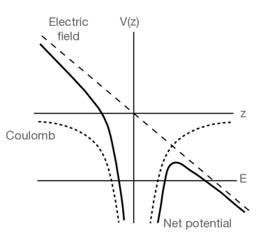
Figure 1: A sketch for the tunneling picture of Schwinger pair production. The Coulomb curves (small-dashed) show the Coulomb attractive potential between the pair of charges; the long dashed line shows the potential energy of the positive charge due to the external electric field, and the solid curves are the sum of the Coulomb and external electric potentials. Quantum fluctuations deep in the potential well with energy E can tunnel out and escape to infinity and would be interpreted as Schwinger particle pairs.

Alternatively, if one adopts temporal gauge, as we shall do, the gauge potential is

$$A^{\mu}=(0,0,0,Et)$$ (3)

Now the gauge field is spatially well-behaved but varies with time. Any quantum excitations of charged fields will obtain time-dependent frequencies, just as for a simple harmonic oscillator with a time-varying spring constant. The charged quantum modes in the vacuum will get excited due to this time-dependent background leading to pair production. The rate of particle production can be calculated using the standard machinery of Bogolyubov coefficients (e.g. Bogolyubov (1958); Birrell and Davies (1984)), or in the framework of the “classical-quantum correspondence” where quantum particle production is described in terms of solutions of the classical equations Vachaspati and Zahariade (2018, 2019).

Here we consider a pure non-Abelian SU(2) gauge theory with a background (“color”) electric field in temporal gauge. In addition, the theory contains “gluon” excitations that are massless and charged. A background electric field that is analogous to that in ordinary electrodynamics is known to pair produce gluons Matinyan and Savvidy (1978); Brown and Weisberger (1979); Yildiz and Cox (1980); Ambjorn and Hughes (1982a, b); Nayak and van Nieuwenhuizen (2005); Cooper and Nayak (2006); Cooper et al. (2008); Nair and Yelnikov (2010); Kim and Schubert (2011); Ilderton (2022); Huet et al. (2014); Ragsdale and Singleton (2017); Karabali et al. (2019); Cardona and Vachaspati (2021). One important difference from the original Schwinger calculation is that the gluons are massless and the exponential suppression in (1) is absent. In fact, there are ultraviolet and infrared divergences as discussed in Ref. Cardona and Vachaspati (2021) that are presumably controlled by asymptotic freedom and confinement. However, it appears that no matter how weak the electric field strength is, there is always some particle production and hence the electric field should decay.

If any non-Abelian electric field decays due to the Schwinger process, it would imply that any external electric charge would get shielded by gluons and the resulting long range electric field would vanish. This runs counter to the picture that QCD has electric flux tubes that confine electric charges, and we are led to the question if there can be non-Abelian electric field configurations that are immune to the Schwinger process, i.e. non-Abelian electric fields that are unexciting. Such electric flux tubes would be models for the QCD string responsible for confinement that have been discussed now for nearly half a century Kogut and Susskind (1974, 1975); Takahashi et al. (2002); Bissey et al. (2007).

A guess for an unexciting non-Abelian electric field configuration was suggested in Ref. Vachaspati (2022). One needs the electric field background to be stationary. Already we have mentioned boosted solitons as unexciting backgrounds. An alternative is to have “rotating” backgrounds. In non-Abelian gauge theories, for example when quantizing magnetic monopole backgrounds, it is known that there are rotor degrees of freedom that, when excited, endow a monopole with electric charge and convert it into a dyon. Could such rotor degrees of freedom be relevant for unexciting non-Abelian electric fields?

Approaching the problem from a different point of view, one wishes to construct “stationary” gauge fields that lead to a uniform electric field. Fortunately this problem has been analyzed in detail in Ref. Brown and Weisberger (1979) and it is found that there are two gauge inequivalent classes of gauge fields that lead to the same non-Abelian electric field. One of these ways is analogous to the Abelian gauge potential, while the second one is necessarily due to the non-Abelian nature of the model. We will explain this in more detail in Sec. III but suffice it to say that this second description of the electric field corresponds precisely to the uniform rotation of a rotor degree of freedom with quantized angular momentum (Sec. V). The analysis of Sec. IV shows explicitly that this gauge background is stationary and does not lead to particle production, and consequently is protected against quantum dissipation. Quantum excitations on top of the classical background will settle into some ground state which is very difficult to determine because of the strongly coupled nature of the system but, whatever the state may be, it will be stationary. In Sec. VII we discuss the simpler quantization of the homogeneous modes in the linearized approximation. Even this limited analysis has some novel features. Most of our analysis is done for a uniform electric field as this is simpler but in Sec. VI we remark on strategies to determine the profile of a flux tube. We start our discussion with a motivating illustration of an unexciting electric field in 1+1D in Sec. II and summarize our conclusions in Sec. VIII.

II An illustrative example in 1+1D

An example of an electric field configuration without Schwinger pair production is already known in massless QED in 1+1 dimensions Chu and Vachaspati (2010); Gold et al. (2021) with action,

$$S=\int d^{2}x\left[{\bar{\psi}}\gamma^{\mu}(i\partial_{\mu}+eA_{\mu})\psi-\frac{1}{4}F_{\mu\nu}F^{\mu\nu}\right]$$ (4)

where $\psi$ is a fermion field, $A_{\mu}$ is a U(1) gauge field, and $F_{\mu\nu}$ is the field strength.

An unexciting electric field background is given by Chu and Vachaspati (2010),

$$F_{01} = Q(\Theta(x+L/2)-\Theta(x-L/2))$$ (5)

$$+g(f(x+L/2)-f(x-L/2))$$

where $g=e/\sqrt{\pi}$ and $Q$ is the external charge on a capacitor with plate separation $L$, and

$$f(x)=-\frac{Q}{2g}{\rm sgn}(x)\left(1-e^{-g|x|}\right).$$ (6)

The terms proportional to $Q$ in (5) give the electric field of the classical capacitor, while the last two terms give the contribution of a quantum condensate of fermions. Quantum effects provide extra sources that screen some of the classical electric field, resulting in a net electric field in which there is no Schwinger pair production.

Similarly in the non-Abelian case discussed below, we consider an electric field configuration that solves the classical equations of motion only in the presence of some sources (see Sec. IV). These sources can be external or be generated internally by quantum effects due to higher order interactions.

III Uniform electric field

As discussed in Brown and Weisberger (1979), a homogeneous non-Abelian electric field can be derived from several gauge inequivalent potentials. Say we want the gauge potentials for an electric field in the third isospin direction and pointing along the $z$ direction, i.e. $E\equiv E^{3}_{z}=W^{3}_{0z}$ where $W^{a}_{\mu}$ are gauge potentials from which the field strength $W^{a}_{\mu\nu}$ is derived in the usual way,

$$W^{a}_{\mu\nu}=\partial_{\mu}W^{a}_{\nu}-\partial_{\nu}W^{a}_{\mu}+\epsilon^{abc}W^{b}_{\mu}W^{c}_{\nu}$$ (7)

where we have set the gauge coupling to unity since we will only be considering non-interacting quantum fluctuations on an electric field background.

The first “trivial” way to obtain $E^{3}_{z}$ is to take,

$$W^{a}_{\mu}=-E\,t\delta^{a3}\partial_{\mu}z$$ (8)

Then

$$E^{a}_{i}\equiv-(\partial_{t}W^{a}_{i}-\partial_{i}W^{a}_{t}+\epsilon^{abc}W^{b}_{t}W^{c}_{i})=E\delta^{a3}\delta_{iz}$$ (9)

A second way to obtain $E^{3}_{z}$ is to take Brown and Weisberger (1979),

$$W^{1}_{\mu}=(\Omega,0,0,0),\ \ W^{2}_{\mu}=(0,0,0,-E/\Omega),\ \ W^{3}_{\mu}=0$$ (10)

where $\Omega$ is a constant (that will turn out to be quantized in Sec. V.) With (10) we also obtain

$$E^{a}_{i}=E\delta^{a3}\delta_{iz}.$$ (11)

Even though the gauge potentials in Eqs. (8) and (10) yield the same field strength, they are gauge inequivalent, as are the gauge fields for different values of $\Omega$, as can be seen by computing other gauge invariant quantities such as Brown and Weisberger (1979),

$$(D_{\nu}W^{\mu\nu})^{a}(D_{\sigma}W^{\ \sigma}_{\mu})^{a}=-E^{2}\left(\Omega^{2}-\frac{E^{2}}{\Omega^{2}}\right)$$ (12)

where

$$(D_{\nu}W^{\mu\nu})^{a}\equiv\partial_{\nu}W^{\mu\nu a}+\epsilon^{abc}W_{\nu}^{b}W^{\mu\nu c}.$$ (13)

Since the gauge invariant quantity on the left-hand side of (12) depends on $\Omega$, gauge fields for different $\Omega$ values are gauge inequivalent. However, the energy density of the configuration is independent of $\Omega$, since the electric field does not depend on $\Omega$.

In the context of “unexciting” backgrounds discussed in Vachaspati (2022), we would like to work in temporal gauge and set $W^{a}_{0}=0$. A gauge transformation yields,

$${\bf W}^{\prime}_{\mu}=U^{-1}{\bf W}_{\mu}U+iU^{-1}\partial_{\mu}U$$ (14)

where now ${\bf W}_{\mu}\equiv W^{a}_{\mu}T^{a}=W^{a}_{\mu}\sigma^{a}/2$, $T^{a}$ are the generators of SU(2) normalized to ${\rm Tr}(T^{a}T^{b})=\delta^{ab}/2$ and $\sigma^{a}$ are the Pauli spin matrices. The gauge transformation $U$ that takes us to temporal gauge is given by,

$$U=e^{i\sigma^{1}\Omega t/2}$$ (15)

Using the identities,

$$e^{i\hat{n}\cdot\sigma\theta} = \cos\theta+i\hat{n}\cdot\sigma\sin\theta$$

$$e^{i\hat{n}\cdot{\vec{\sigma}}\theta}{\vec{\sigma}}e^{-i\hat{n}\cdot{\vec{\sigma}}\theta} = {\vec{\sigma}}\cos(2\theta)+{\hat{n}}\times{\vec{\sigma}}\sin(2\theta)$$ (16)

$$+{\hat{n}}\,{\hat{n}}\cdot{\vec{\sigma}}(1-\cos(2\theta))$$

we find

$$W^{1}_{\mu}{}^{\prime} = 0$$

$$W^{2}_{\mu}{}^{\prime} = -\frac{E}{\Omega}\cos(\Omega t)\partial_{\mu}z,$$

$$W^{3}_{\mu}{}^{\prime} = -\frac{E}{\Omega}\sin(\Omega t)\partial_{\mu}z.$$ (17)

A global SU(2) rotation can be used to bring the gauge fields to a form that we will use

$$W^{1}_{\mu} = -\frac{E}{\Omega}\cos(\Omega t)\partial_{\mu}z,$$

$$W^{2}_{\mu} = -\frac{E}{\Omega}\sin(\Omega t)\partial_{\mu}z,$$

$$W^{3}_{\mu} = 0$$ (18)

and we have dropped the primes for convenience.

Ref. Brown and Weisberger (1979) wrote the gauge field in the form of (10) to show that the same electric field can be obtained with a one parameter ($\Omega$) family of gauge inequivalent gauge fields. We are only interested in a fixed value of $\Omega$ and it is more convenient to write the non-vanishing components as

$$W^{1}_{\mu}=-\epsilon\cos(\Omega t)\partial_{\mu}z,\ W^{2}_{\mu}=-\epsilon\sin(\Omega t)\partial_{\mu}z.$$ (19)

Then the electric field is given by

$$E=\Omega\epsilon.$$ (20)

Equivalently, we can work with $W^{\pm}_{\mu}\equiv W^{1}_{\mu}\pm iW^{2}_{\mu}$,

$$W^{\pm}_{\mu}=-\epsilon e^{\pm i\Omega t}\partial_{\mu}z,\ \ W^{3}_{\mu}=0.$$ (21)

Defining

$$W_{\mu\nu}^{\pm}=W_{\mu\nu}^{1}\pm iW_{\mu\nu}^{2}$$ (22)

we find

$$W_{\mu\nu}^{\pm}=\partial_{\mu}W_{\nu}^{\pm}-\partial_{\nu}W_{\mu}^{\pm}\pm i(W_{\mu}^{3}W_{\nu}^{\pm}-W_{\nu}^{3}W_{\mu}^{\pm})$$ (23)

and

$$W_{\mu\nu}^{3}=\partial_{\mu}W_{\nu}^{3}-\partial_{\nu}W_{\mu}^{3}+\frac{i}{2}(W_{\mu}^{+}W_{\nu}^{-}-W_{\nu}^{+}W_{\mu}^{-}).$$ (24)

For the background in (18) we get,

$$W_{\mu\nu}^{\pm}=\mp iE(\partial_{\mu}t\,\partial_{\nu}z-\partial_{\nu}t\,\partial_{\mu}z)e^{\pm i\Omega t},\ \ W_{\mu\nu}^{3}=0$$ (25)

The Lagrangian density for the non-Abelian gauge sector is

$${\cal L}_{g}=-\frac{1}{4}\left[W_{\mu\nu}^{+}W^{\mu\nu-}+W_{\mu\nu}^{3}W^{\mu\nu 3}\right]$$ (26)

The full model will necessarily include a Lagrangian density for external sources and their couplings to the gauge fields as we will discuss in Sec. IV.

The important lesson of this section is that in non-Abelian gauge theories we have several gauge inequivalent choices for the gauge potential corresponding to an electric field background. The gauge potential of interest to us is time-dependent only because it is rotating in gauge field space as in (21).

IV Expansion around a flux tube background

We now consider the electric field configuration in (18) as a background and denote it by $A_{\mu}$. We assume it is produced by some unspecified external sources, and we wish to determine if it leads to Schwinger pair creation. We write

$$W_{\mu}^{\pm}=A_{\mu}^{\pm}+e^{\pm i\Omega t}Q_{\mu}^{\pm},\ \ W_{\mu}^{3}=A_{\mu}^{3}+Q_{\mu}^{3}$$ (27)

where now $A_{\mu}^{a}$ includes an unspecified radial profile function, $f(r)$, ($r=\sqrt{x^{2}+y^{2}}$),

$$A^{\pm}_{\mu}=-\epsilon e^{\pm i\Omega t}f(r)\,\partial_{\mu}z,\ \ A^{3}_{\mu}=0,$$ (28)

and $Q_{\mu}^{a}$ are quantum excitations around the background. More explicitly,

$$W_{\mu}^{\pm}=e^{\pm i\Omega t}\left(-\epsilon f(r)\,\partial_{\mu}z+Q_{\mu}^{\pm}\right),\ \ W_{\mu}^{3}=Q_{\mu}^{3}$$ (29)

Then

$$W_{\mu\nu}^{\pm} = e^{\pm i\Omega t}\bigl{[}{\mathscr{A}}_{\mu\nu}^{\pm}+({\mathscr{D}}_{\mu}Q_{\nu}^{\pm}-{\mathscr{D}}_{\nu}Q_{\mu}^{\pm})$$ (30)

$$\hskip 56.9055pt\pm i(Q_{\mu}^{3}Q_{\nu}^{\pm}-Q_{\nu}^{3}Q_{\mu}^{\pm})\bigr{]}$$

where

$${\mathscr{A}}_{\mu\nu}^{\pm} \equiv \pm iEf(r)(\partial_{\mu}z\partial_{\nu}t-\partial_{\nu}z\partial_{\mu}t)$$ (31)

$$\hskip 42.67912pt+\epsilon f^{\prime}(r)(\partial_{\mu}z\partial_{\nu}r-\partial_{\nu}z\partial_{\mu}r),$$

$${\mathscr{D}}_{\mu}Q_{\nu}^{\pm}\equiv\partial_{\mu}Q_{\nu}^{\pm}\pm i\Omega\partial_{\mu}t\,Q_{\nu}^{\pm}\pm i\epsilon f(r)\partial_{\mu}z\,Q_{\nu}^{3}.$$ (32)

We also have

$$W_{\mu\nu}^{3}={\mathscr{D}}_{\mu}Q_{\nu}^{3}-{\mathscr{D}}_{\nu}Q_{\mu}^{3}+\frac{i}{2}(Q_{\mu}^{+}Q_{\nu}^{-}-Q_{\nu}^{+}Q_{\mu}^{-})$$ (33)

with

$${\mathscr{D}}_{\mu}Q_{\nu}^{3} \equiv \partial_{\mu}Q_{\nu}^{3}+i\frac{\epsilon}{2}f(r)\partial_{\mu}z\,Q_{\nu}^{+}-i\frac{\epsilon}{2}f(r)\partial_{\mu}z\,Q_{\nu}^{-}$$ (34)

$$= \partial_{\mu}Q_{\nu}^{3}-\epsilon f(r)\partial_{\mu}zQ_{\nu}^{2}$$

The Lagrangian density for $Q^{a}_{\mu}$ is evaluated from (26),

$${\cal L}_{g} = -\frac{1}{4}\biggl{|}{\mathscr{A}}_{\mu\nu}^{+}+({\mathscr{D}}_{\mu}Q_{\nu}^{+}-{\mathscr{D}}_{\nu}Q_{\mu}^{+})$$ (35)

$$\hskip 71.13188pt+i(Q_{\mu}^{3}Q_{\nu}^{+}-Q_{\nu}^{3}Q_{\mu}^{+})\biggr{|}^{2}$$

$$\hskip-14.22636pt-\frac{1}{4}\biggl{|}{\mathscr{D}}_{\mu}Q_{\nu}^{3}-{\mathscr{D}}_{\nu}Q_{\mu}^{3}+\frac{i}{2}(Q_{\mu}^{+}Q_{\nu}^{-}-Q_{\nu}^{+}Q_{\mu}^{-})\biggr{|}^{2}$$

The Lagrangian density (35) describes the interaction of $Q_{\mu}^{a}$ with the background $A_{\mu}$. Even at this stage it is clear that there can be no particle production: the background dependent terms in (35), for example ${\mathscr{A}}_{\mu\nu}^{\pm}$ and in ${\mathscr{D}}_{\mu}Q_{\nu}^{a}$, are all independent of time and there is no $z-$dependence either. For Schwinger pair production, the gauge field background should either have non-trivial time-dependence or it should have non-trivial spatial dependence, as discussed in Sec. I. The interactions of $Q_{\mu}^{a}$ with the background will lead to a non-trivial ground state wavefunctional but without any time-dependent excitations. Hence the electric-magnetic field background in (31) is “unexciting”.

We will now examine the system more explicitly by expanding the Lagrangian density in powers of $Q$.

IV.1 First order Lagrangian density

The Lagrangian density up to linear order terms in $Q$ is,

$${\cal L}_{g}^{(1)} = -\frac{1}{4}\mathscr{A}_{\mu\nu}^{+}\bigl{(}{\mathscr{D}}^{\mu}Q^{\nu+}-{\mathscr{D}}^{\nu}Q^{\mu+}\bigr{)}^{*}+{\rm c.c.}$$ (36)

$$\to +\frac{1}{2}({\mathscr{D}}^{\mu}\mathscr{A}_{\mu\nu}^{+})Q^{\nu-}+{\rm c.c.}$$

where in the second line we have dropped total derivative terms. The linear order variation doesn’t vanish; neither do they for the illustrative example in (5) since there are external sources for the electric field and quantum effects induce a condensate of sources. Here we simply supplement this linear order Lagrangian density with a source term that couples external currents, $j_{\mu}^{a}$, to $W_{\mu}^{a}$,

$${\cal L}_{s}=j_{\mu}^{a}W^{\mu a}=j_{\mu}^{a}A^{\mu a}+e^{\pm i\Omega t}j_{\mu}^{\mp}Q^{\mu\pm}+j_{\mu}^{3}Q^{\mu 3}$$ (37)

The external current includes sources that are necessary to generate the background net flux of electric field. The currents can also contain effective quantum contributions that arise due to higher order interactions as these backreact at the linear level (see Sec. II). Here we simply assume the existence of such a current without any dynamical explanation.

Requiring that the linear order terms vanish up to total derivatives gives,

$$j_{\mu}^{\pm} = -\frac{\epsilon}{2}e^{\pm i\Omega t}\left(f^{\prime\prime}+\frac{f^{\prime}}{r}+\Omega^{2}f\right)\partial_{\mu}z,$$

$$j_{\mu}^{3} = -\Omega\epsilon^{2}f^{2}\,\partial_{\mu}t.$$ (38)

These currents do not include the external sources located at $z=\pm\infty$. To see this it is most transparent to consider the Abelian case of a homogeneous electric field with field strength tensor

$$F_{\mu\nu}=E(\partial_{\mu}t\partial_{\nu}z-\partial_{\nu}t\partial_{\mu}z).$$ (39)

Insertion into Maxwell’s equations gives

$$j_{\mu}=-\partial^{\nu}F_{\nu\mu}=0$$ (40)

and the charged capacitor plates at $z=\pm\infty$ are not included in $j_{\mu}$.

Since the currents in (38) do not include the asymptotic sources, they must arise entirely as a quantum condensate similar to the second line in (5). To show that such a condensate arises due to the strong interactions is difficult but some progress may be made in the semiclassical approximation. We start with the equation of motion for the gauge fields,

$$D_{\nu}W^{\nu\mu a}=0$$ (41)

where the covariant derivative is defined in (13). We then substitute

$$W_{\mu}^{a}=A_{\mu}^{a}+q_{\mu}^{a}$$ (42)

in (41) where $A^{\mu a}$ is classical while $q^{\mu a}$ is quantum. The operator equation (41) is replaced by its ground state expectation value. If we assume that expectation values of odd powers of $q^{\mu a}$ vanish, some algebra yields,

$$D_{\nu}^{(A)}A^{\nu\mu a}=-j^{\mu a}$$ (43)

where $D_{\nu}^{(A)}A^{\nu\mu a}$ is as in (13) with $W$ replaced by $A$ and

$$j^{\mu a} \equiv \epsilon^{abc}\langle\partial_{\nu}q^{\nu b}q^{\mu c}-q^{\nu b}\partial^{\mu}q_{\nu}^{c}+2q^{\nu b}\partial_{\nu}q^{\mu c}\rangle_{R}$$ (44)

$$+A_{\nu}^{b}\langle q^{\nu a}q^{\mu b}-2q^{\nu b}q^{\mu a}\rangle_{R}+A_{\nu}^{a}\langle q^{\nu b}q^{\mu b}\rangle_{R}$$

$$+A^{\mu b}\langle q^{b}_{\nu}q^{\nu a}\rangle_{R}-A^{\mu a}\langle q_{\nu}^{b}q^{\nu b}\rangle_{R}$$

The symbol $\langle\cdot\rangle_{R}$ refers to the renormalized vacuum expectation value. One possible renormalization scheme would be to subtract out the expectation value in the trivial vacuum with zero electric field,

$$\langle{\cal O}\rangle_{R}=\langle{\cal O}\rangle-\langle{\cal O}\rangle_{\epsilon=0}$$ (45)

for any quantum operator ${\cal O}$. To illustrate how the current might result in a charge condensate, consider the $\mu=0$, $a=3$ component of (44). Since we are working in temporal gauge and $q_{\mu}^{a}$ is defined in terms of $Q_{\mu}^{a}$ using (27), the expression simplifies, and we get

$$j^{(3)}_{0} = \Omega\langle(Q_{i}^{(1)})^{2}+(Q_{i}^{(2)})^{2}\rangle_{R}$$ (46)

$$+\langle Q_{i}^{(1)}{\dot{Q}}_{i}^{(2)}-Q_{i}^{(2)}{\dot{Q}}_{i}^{(1)}\rangle_{R}$$

Assuming the ground state of $Q_{\mu}^{a}$ has zero “angular momentum” (also see Sec. VII), we get a charge density,

$$j^{(3)}_{0}=\Omega\langle(Q_{i}^{(1)})^{2}+(Q_{i}^{(2)})^{2}\rangle_{R}.$$ (47)

This can be compared to (38) and for a homogeneous electric field ($f=1$) we have,

$$\epsilon^{2}=-\langle(Q_{i}^{(1)})^{2}+(Q_{i}^{(2)})^{2}\rangle_{R}.$$ (48)

Note that the right-hand side can be positive due to the definition in (45).

In summary, the background need not satisfy the classical equations of motion; instead it is more realistic to ask if the background satisfies the semiclassical equations of motion. By examining the semiclassical equations, we discover that quantum effects can indeed provide appropriate sources for the electric field background under consideration.

IV.2 Second order Lagrangian density

The quadratic order Lagrangian density is,

$${\cal L}_{g}^{(2)} = -\frac{1}{4}\bigl{|}{\mathscr{D}}_{\mu}Q_{\nu}^{+}-{\mathscr{D}}_{\nu}Q_{\mu}^{+}\bigr{|}^{2}-\frac{1}{4}\bigl{|}{\mathscr{D}}_{\mu}Q_{\nu}^{3}-{\mathscr{D}}_{\nu}Q_{\mu}^{3}\bigr{|}^{2}$$ (49)

$$+\frac{i}{4}\left[\mathscr{A}_{\mu\nu}^{+}(Q^{\mu 3}Q^{\nu-}-Q^{\nu 3}Q^{\mu-})-c.c.\right].$$

or, explicitly,

$$\hskip-21.33955pt{\cal L}_{g}^{(2)}=$$ (50)

$$\frac{1}{2}({\dot{Q}}^{(1)}_{i}-\Omega Q^{(2)}_{i})^{2}+\frac{1}{2}({\dot{Q}}^{(2)}_{i}+\Omega Q^{(1)}_{i})^{2}+\frac{1}{2}({\dot{Q}}^{(3)}_{i})^{2}$$

$$- \frac{1}{4}(\partial_{i}Q^{(1)}_{j}-\partial_{j}Q^{(1)}_{i})^{2}$$

$$- \frac{1}{4}(\partial_{i}Q^{(2)}_{j}-\partial_{j}Q^{(2)}_{i}+\epsilon f({\hat{z}}_{i}Q^{(3)}_{j}-{\hat{z}}_{j}Q^{(3)}_{i}))^{2}$$

$$- \frac{1}{4}(\partial_{i}Q^{(3)}_{j}-\partial_{j}Q^{(3)}_{i}-\epsilon f({\hat{z}}_{i}Q^{(2)}_{j}-{\hat{z}}_{j}Q^{(2)}_{i}))^{2}$$

$$+ \epsilon f^{\prime}({\hat{z}}_{i}{\hat{r}}_{j}-{\hat{z}}_{j}{\hat{r}}_{i})Q^{(2)}_{i}Q^{(3)}_{j}$$

where $Q^{\pm}_{i}=Q^{(1)}_{i}\pm iQ^{(2)}_{i}$, ${\hat{z}}_{i}$, ${\hat{r}}_{i}$ are unit vectors in the $z-$ and $r-$ directions, and the contraction of spatial indices is with the Kronecker delta, e.g. $({\dot{Q}}^{(3)}_{i})^{2}={\dot{Q}}^{(3)}_{i}{\dot{Q}}^{(3)}_{i}$.

Denoting the momentum conjugate to $Q^{a}_{i}$ by $P^{a}_{i}$, the Hamiltonian density corresponding to ${\cal L}_{g}^{(2)}$ is,

$$\hskip-21.33955pt{\cal H}_{g}^{(2)}=\frac{1}{2}(P^{(a)}_{i})^{2}+\frac{1}{4}(\partial_{i}Q^{(1)}_{j}-\partial_{j}Q^{(1)}_{i})^{2}$$ (51)

$$+ \frac{1}{4}(\partial_{i}Q^{(2)}_{j}-\partial_{j}Q^{(2)}_{i}+\epsilon f({\hat{z}}_{i}Q^{(3)}_{j}-{\hat{z}}_{j}Q^{(3)}_{i}))^{2}$$

$$+ \frac{1}{4}(\partial_{i}Q^{(3)}_{j}-\partial_{j}Q^{(3)}_{i}-\epsilon f({\hat{z}}_{i}Q^{(2)}_{j}-{\hat{z}}_{j}Q^{(2)}_{i}))^{2}$$

$$- \epsilon f^{\prime}({\hat{z}}_{i}{\hat{r}}_{j}-{\hat{z}}_{j}{\hat{r}}_{i})Q^{(2)}_{i}Q^{(3)}_{j}+{\cal J}$$

where,

$${\cal J}=\Omega(Q^{(2)}_{i}P^{(1)}_{i}-Q^{(1)}_{i}P^{(2)}_{i})$$ (52)

is an “angular momentum” term.

To check that the background is unexciting, we simply note that the Hamiltonian density does not have any time-dependence. If we decompose the field into eigenmodes, the amplitude of each eigenmode is a quadratic variable that behaves like a simple harmonic oscillator variable with possibly an angular momentum contribution to the Hamiltonian (see Sec. VII).

One potential complication is if the diagonalization of the second order Hamiltonian density, ${\cal H}_{g}^{(2)}$, leads to modes that have imaginary frequencies, i.e. are simple harmonic oscillators with inverted potentials. An analysis of the spectrum of frequencies was carried out in Ref. Bazak and Mrowczynski (2022) for the special choice $\Omega=\sqrt{E}$ and the authors found some unstable modes. These unstable modes imply that the quantum ground state of the $Q^{a}_{i}$ will be something other than the simple harmonic oscillator ground states (at least for this choice of $\Omega$). The instability will be tamed by the higher order interactions. Since the higher order Lagrangian density is also time-independent (see Subsection. IV.3 below), there can be no particle production and the electric field background is protected against quantum dissipation. However the danger is that the expectation value of the quantum excitations might not vanish and then the separation between the classical background, $A_{\mu}^{a}$, and the quantum excitations becomes unclear. The idea behind postulating $A_{\mu}^{a}$ as a background is that the quantum excitations are small and their expectation values vanish. For this to happen, the background should not have any instabilities. The stability analysis deserves to be investigated for the entire range of parameters.

To evaluate the quantum state of the $Q^{a}_{i}$ in the full interacting theory is beyond the scope of the present work, but we discuss the simpler problem of the quantum state for homogeneous modes in the quadratic Hamiltonian in Sec. VII.

IV.3 Higher order Lagrangian density

For completeness we also give the cubic and quartic order terms in the Lagrangian density,

$${\cal L}_{g}^{(3+4)} = \frac{i}{4}\biggl{[}({\mathscr{D}}_{i}Q_{j}^{+}-{\mathscr{D}}_{j}Q_{i}^{+})(Q_{i}^{3}Q_{j}^{-}-Q_{j}^{3}Q_{i}^{-})$$ (53)

$$\hskip-28.45274pt+\frac{1}{2}({\mathscr{D}}_{i}Q_{j}^{3}-{\mathscr{D}}_{j}Q_{i}^{3})(Q_{i}^{+}Q_{j}^{-}-Q_{j}^{+}Q_{i}^{-})-c.c.\biggr{]}$$

$$\hskip-49.79231pt-\frac{1}{4}\bigl{|}Q_{i}^{3}Q_{j}^{+}-Q_{j}^{3}Q_{i}^{+}\bigr{|}^{2}-\frac{1}{16}\bigl{|}Q_{i}^{+}Q_{j}^{-}-Q_{j}^{+}Q_{i}^{-}\bigr{|}^{2}$$

To summarize Sec. IV, the electric field background (28) is unexciting. There will be quantum fluctuations around this background and they will be in some stationary quantum ground state but particle production will be absent. For this reason, the electric field background is stable to quantum dissipation.

V Symmetry and quantization

As discussed in the introduction, a static soliton can be boosted to give a time-dependent background but this will not lead to particle production. This is because the static soliton has translational symmetry and a boosted soliton provides time dependence to the background but the excitation frequencies are still time-independent. In other words, the boosted soliton is a “stationary” background. Similarly, there should be a symmetry of the non-Abelian gauge theory, and the electric field background we have been discussing should be due to a time-dependence in the symmetry variables. The situation is very similar to the symmetries of monopoles and the rotor degree of freedom that leads to dyons, discussed for example in Refs. Julia and Zee (1975); Callan (1982) and extensively in Section 2.7 of Preskill (1987).

Consider the global gauge transformation

$$W_{\mu}^{\pm}\to W^{\prime}_{\mu}{}^{\pm}=e^{\pm i\theta}W_{\mu}^{\pm},\ \ W_{\mu}^{3}\to W^{\prime}_{\mu}{}^{3}=W_{\mu}^{3}$$ (54)

where $\theta$ is a constant parameter. The boosted soliton background corresponds in this case to promoting the rotor degree of freedom: $\theta\to\theta(t)$.

Next let

$$W_{\mu}^{\pm}=e^{\pm i\theta}v_{\mu}^{\pm},\ \ W_{\mu}^{3}=v_{\mu}^{3}$$ (55)

where $v_{0}^{a}=0$ in temporal gauge and we also assume that the $v_{\mu}^{a}$ background is static (just like the static soliton). The angular variable $\theta$ is assumed to only depend on time. Substituting (55) in the Lagrangian for $W_{\mu}^{a}$ (i.e. (26) integrated over space) gives the Lagrangian for $\theta$,

$$L_{\theta}=\frac{1}{2}I{\dot{\theta}}^{2}$$ (56)

where the “moment of inertia” is

$$I=\int d^{3}x|v_{i}^{+}|^{2}.$$ (57)

Solving for the quantum dynamics of $\theta$ is straightforward and leads to the quantization of angular momentum and correspondingly

$$\Omega={\dot{\theta}}=\frac{l}{I},\ \ l=0,\pm 1,\pm 2,\ldots$$ (58)

Thus the parameter $\Omega$ is quantized. The electric field strength is also quantized as

$$E=\Omega\epsilon=\frac{\epsilon}{I}l.$$ (59)

The quantum number $l$ has the interpretation of the number of charge quanta. To see this we evaluate the total charge, $q^{a}$, by integrating the $\mu=0$ component of (38) over a volume $V$ for the homogeneous case ($f=1$). This gives

$$q^{a}=-V\Omega\epsilon^{2}\delta^{a3}=-l\delta^{a3}$$ (60)

in units where the gauge coupling constant $g=1$ and we have used (58) and $I=\epsilon^{2}V$.

VI Flux tube profile

The quantum state of the fluctuations $Q^{a}_{i}$ will depend on the profile $f(r)$. If we know the quantum state, we can calculate the expectation value of the Hamiltonian, $\langle H\rangle$, for the choice of $f(r)$. If $\langle H\rangle$ is minimized for some $f(r)$, subject to a suitable constraint on the background electric field, it would specify the profile of the electric field flux tube and its tension. We can define the background electric flux as

$$\Phi^{\pm}\equiv\int d^{2}x\,{\mathscr{A}}_{0z}^{\pm}=\mp iEe^{\pm i\Omega t}\int d^{2}x\,f(r),$$ (61)

with ${\mathscr{A}}_{\mu\nu}^{\pm}$ given in (31) and $\Phi^{3}=0$. The flux itself is not gauge invariant but, having chosen a fixed form of the background gauge fields, one can restrict the class of functions in this background gauge. This amounts to exploring profile functions for which the integral on the right-hand side of (61) is unity,

$$2\pi\int dr\,rf(r)=1.$$ (62)

Unfortunately, there is no simple way to find the quantum state of $Q^{a}_{i}$ for given $f(r)$, especially as the fluctuations are strongly interacting. The only hope seems to be to determine $f(r)$ numerically, using lattice techniques.

VII Quantum state of the homogeneous modes

We now consider the Hamiltonian density in (51) for homogeneous excitations on a uniform electric field background. Then $\partial_{i}Q^{a}_{j}=0$ and $f=1$, and the Hamiltonian is related to the Hamiltonian density by suitable factors of the spatial volume $V$,

$$\hskip-21.33955ptH_{g}^{(2)}=\frac{1}{2V}(P^{(a)}_{i})^{2}+\frac{\epsilon^{2}V}{4}({\hat{z}}_{i}Q^{(3)}_{j}-{\hat{z}}_{j}Q^{(3)}_{i})^{2}$$

$$\hskip-24.18501pt+\frac{\epsilon^{2}V}{4}({\hat{z}}_{i}Q^{(2)}_{j}-{\hat{z}}_{j}Q^{(2)}_{i})^{2}+\Omega(Q^{(2)}_{i}P^{(1)}_{i}-Q^{(1)}_{i}P^{(2)}_{i})$$ (63)

The Hamiltonian then can be written as a sum of six sub-Hamiltonians,

$$H_{1} = \frac{1}{2V}(P^{(1)}_{x})^{2}+\frac{1}{2V}(P^{(2)}_{x})^{2}+\frac{\epsilon^{2}V}{2}(Q^{(2)}_{x})^{2}$$ (64)

$$\hskip 28.45274pt+\Omega(Q^{(2)}_{x}P^{(1)}_{x}-Q^{(1)}_{x}P^{(2)}_{x})$$

$$H_{2} = \frac{1}{2V}(P^{(3)}_{x})^{2}+\frac{\epsilon^{2}V}{2}(Q^{(3)}_{x})^{2}$$ (65)

$$H_{3} = \frac{1}{2V}(P^{(1)}_{y})^{2}+\frac{1}{2V}(P^{(2)}_{y})^{2}+\frac{\epsilon^{2}V}{2}(Q^{(2)}_{y})^{2}$$ (66)

$$\hskip 28.45274pt+\Omega(Q^{(2)}_{y}P^{(1)}_{y}-Q^{(1)}_{y}P^{(2)}_{y})$$

$$H_{4} = \frac{1}{2V}(P^{(3)}_{y})^{2}+\frac{\epsilon^{2}V}{2}(Q^{(3)}_{y})^{2}$$ (67)

$$H_{5} = \frac{1}{2V}(P^{(1)}_{z})^{2}+\frac{1}{2V}(P^{(2)}_{z})^{2}$$ (68)

$$\hskip 28.45274pt+\Omega(Q^{(2)}_{z}P^{(1)}_{z}-Q^{(1)}_{z}P^{(2)}_{z})$$

$$H_{6} = \frac{1}{2V}(P^{(3)}_{z})^{2}$$ (69)

The Hamiltonians $H_{2}$ and $H_{4}$ correspond to simple harmonic oscillators, while $H_{6}$ is that of a free particle. Their eigenstates are well-known; the simple harmonic oscillators states are all bound, while the free particle only has continuum states. $H_{5}$ is the Hamiltonian for a free particle in two dimensions but with an additional angular momentum term, while $H_{1}$ and $H_{3}$ are identical in structure and can also be thought of as a particle in two dimensions with an angular momentum term plus an anisotropic potential. Thus we only need to consider $H_{1}$ and $H_{5}$.

Let us consider $H_{5}$ first and write it in a less cumbersome way,

$$H_{5}\to\frac{1}{2}\pi_{x}^{2}+\frac{1}{2}\pi_{y}^{2}+\Omega(y\pi_{x}-x\pi_{y})$$ (70)

where $\pi_{x}$ and $\pi_{y}$ are momenta conjugate to $x$ and $y$, and we have also chosen units so that $V=1$. One can check that

$$[y\pi_{x}-x\pi_{y},H_{5}]=0$$ (71)

and there are simultaneous eigenstates of the angular momentum operator, $y\pi_{x}-x\pi_{y}$, and $H_{5}$. Defining polar coordinates in the usual way

$$x=r\,\cos\theta,\ \ y=r\,\sin\theta$$ (72)

the energy eigenstates (up to an overall normalization factor) are given in terms of Bessel functions,

$$\psi(r,\theta,t)=Ce^{-i{\cal E}t}J_{l}\left(\sqrt{2({\cal E}+\Omega m)}\,r\right)e^{im\theta},$$ (73)

with $m=0,\pm 1,\pm 2,\ldots$, $C$ is a normalization constant, and the energy, ${\cal E}$, is constrained by ${\cal E}+\Omega m\geq 0$.

An interesting point is that ${\cal E}$ can be negative. In fact, for $\Omega>0$ and $m\to\infty$, ${\cal E}$ can be arbitrarily negative. We expect that when the quartic interactions are taken into account, the energy may get bounded from below. For example, if the interactions effectively provide a mass to the homogeneous mode, we could consider a rotationally symmetric simple harmonic oscillator in 2D with an additional angular momentum term

$$H_{\rm e.g.}=\frac{1}{2}\pi_{x}^{2}+\frac{1}{2}\pi_{y}^{2}+\frac{\mu^{2}}{2}(x^{2}+y^{2})+\Omega(y\pi_{x}-x\pi_{y}),$$ (74)

As the system has rotational symmetry, the angular momentum is still conserved. The Schrodinger problem can be solved in polar coordinates by elementary means to obtain the energy eigenvalues,

$$E_{nm} = (n+|m|+1)\mu-\Omega m,$$ (75)

$$n=0,1,2,\ldots;\ \ m=0,\pm 1,\pm 2,\ldots$$

Consider the case $\Omega>0$. Then, for fixed $n$ and $m\to+\infty$, we have $E_{nm}\to(\mu-\Omega)m$, and the energy is bounded from below only if $\mu\geq\Omega$. Considering that $\Omega$ can have either sign, the condition for the energy to be bounded from below is,

$$\mu\geq|\Omega|$$ (76)

and then the ground state is for $n=m=0$ with energy $\mu$.

In the notation of (70), $H_{1}$ can be written as

$$H_{1}\to\frac{1}{2}\pi_{x}^{2}+\frac{1}{2}\pi_{y}^{2}+\Omega(y\pi_{x}-x\pi_{y})+\frac{\epsilon^{2}}{2}y^{2}$$ (77)

The last term breaks rotational symmetry in the $xy-$plane and the angular dependence will not be given by angular momentum eigenstates as in (73). The wavefunction will now be peaked on the $x-$axis; it will be bounded in the $y-$direction while remaining unbounded in the $x-$direction.

In principle, we can also treat the case of inhomogeneous excitations since the Hamiltonian is quadratic. However, the diagonalization will be technically difficult and the angular momentum term may resist complete diagonalization as in the case of (77).

In this section we have discussed quantum aspects of the homogeneous quantum excitations. The energy spectrum for some of these homogeneous excitations is unbounded from below. If higher order interaction terms effectively give masses to these excitation modes, the spectrum gets bounded provided the mass is greater than $|\Omega|$ (see (76)).

VIII Conclusions

We have found that an electric field in pure non-Abelian SU(2) gauge theory can be stable against quantum dissipation to Schwinger pair production. (Similar constructions can be embedded in theories with larger gauge groups.) This is because the gauge fields underlying the electric field can be chosen as a stationary background in which a rotor degree of freedom is rotating with fixed, quantized, angular momentum in internal space. The quantum state of excitations on this stationary background is also stationary and there is no particle production and no dissipation. This resolves a conundrum that one might intuit from the case of Abelian electric fields, where the electric field dissipates due to pair production, even if at an exponentially suppressed rate. If the same conclusion applied to non-Abelian electric fields, QCD flux tubes would be susceptible to decay due to Schwinger pair production of gluons. Thus we conjecture that QCD flux tubes should be described by gauge fields as given in Eq. (28). If we start with a non-Abelian electric field that is in the Abelian configuration of (8), a guess is that it would evolve into the unexciting non-Abelian configuration of (28).

The existence of stable non-Abelian electric fields opens up a number of related questions. One issue we faced is that we had to postulate classical external charges to source the background electric field. At present it is not known whether such sources need to be external or if they can arise due to the strong interactions as discussed in Sec. IV.1. The key open question is to determine properties of the ground state of quantum excitations around the background electric field. In Sec. IV.2 we have already pointed out the danger posed by unstable modes as then the separation between a classical background and quantum fluctuations is not clear. Assuming that there is a range of parameters where there are no unstable modes, there will be a well-defined ground state which will depend on the profile of the electric field flux tube. Perhaps there are lattice techniques that can determine the optimum flux tube profile for which the overall energy is minimized. The quantum state can also settle the question whether the sources necessary for the stationary background can arise from the internal dynamics of quantum excitations. These are fascinating but difficult questions that we hope to examine in the future.

Another system of interest is that of dyons that carry non-Abelian electric charge, as these can also arise as stationary solutions of non-Abelian Yang-Mills-Higgs theories. We expect such dyons to be stable to Schwinger particle production of non-Abelian gauge bosons but a detailed analysis might yield surprises especially for large $\Omega$, as in the discussion in Sec. VII.