Growth at high substrate coverage can decrease the grain boundary roughness of 2D materials

Abstract

Grain boundary roughness can affect electronic and mechanical properties of two-dimensional materials. This roughness depends crucially on the growth process by which the two-dimensional material is formed. To investigate the key mechanisms that govern the roughness, we have performed kinetic Monte Carlo simulations of a simple model that includes particle attachment, detachment, and diffusion. We have studied the closure of the gap between two flakes during growth, and the subsequent formation of the grain boundary (GB) for a broad range of model parameters. The well known near-equilibrium (attachment-limited) and unstable (diffusion-limited) growth regimes are identified, but we also observe a third regime when the precursor flux is sufficiently high to fully cover the gap between the edges. This high coverage regime forms GBs with spatially uncorrelated roughness, which quickly relax to smoother configurations. Extrapolating the numerical results (with support from a theoretical approach) to edge lengths and gap widths of some micrometers, we confirm the advantage of this regime to produce GBs with minimal roughness faster than near-equilibrium conditions. This suggests an unexpected route towards efficient growth of two-dimensional materials with smooth GBs.

1 Introduction

The variety of applications of two-dimensional (2D) materials such as graphene and transition metal dichalcogenides has motivated several studies of their growth kinetics in the last two decades [1, 2, 3, 4, 5]. The growth of large grains is frequently desired to reduce the effects of grain boundaries (GBs) on the electronic and mechanical properties. However, in some materials, a large GB density may be a minor problem; this is the case for the integration of ultrathin $\text{Mo}\text{S}_{2}$ films with Si substrates in some devices that require low temperature deposition [6]. Moreover, large GB densities may be beneficial for some applications of 2D materials, such as $\text{W}\text{S}_{2}$ in sensors of Hg [7] and $\text{Mo}\text{S}_{2}$ in the production of memtransistors [8]. GBs of $\text{W}\text{S}_{2}$ may also be useful as high conductivity channels [9].

Beyond the GB density, the GB roughness may also affect the properties of 2D materials in nontrivial ways. Sinusoidal graphene GBs are advantageous over atomically flat GBs because they increase the mechanical strength and improve electronic properties [10]. The fractures of $\text{Re}\text{S}_{2}$ monolayers more easily occur at GBs parallel to Re chains [11], so that disordered GBs may improve their properties. In the case of graphene, there is also evidence that the grain size at the micrometer scale does not have relevant effects on the electric conductivity [12] and that the mechanical strength is not reduced in the presence of GBs [13].

The GB morphology is strongly related to the growth conditions and several models were already proposed to explain this relation [1, 3]. For sufficiently slow graphene growth, the so-called attachment limited (or near-equilibrium) conditions are observed, which usually lead to formation of smooth GBs. Models of step flow describe the edge propagation [14] and the GB structure can be determined by the misorientation angle [15] in these conditions. Similar models and other multi-scale approaches are used to describe the growth of 2D metal dichalcogenides [16, 17, 18]. However, fast growth is frequently important for applications. In this case, the so-called diffusion limited regime is frequently observed, in which GBs significantly deviate from a straight profile. Experiments, phase field models, and kinetic Monte Carlo (kMC) simulations show formation of grains with fractal or dendritic morphologies that reproduce experimental observations [19, 20, 21, 3, 22, 23, 17].

The recurrent observation of similar relations between the GB morphology and the growth conditions in a wide variety of materials is a motivation for the study of models that only contain the essential physico-chemical mechanisms that are needed to explain those relations. This reasoning has already been successful in the description of the morphology of homoepitaxial metal and semiconductor films by means of generic models including adatom diffusion and attachment/detachment from islands and terraces [24, 25, 26, 27, 28, 29].

In this work, we introduce a model for the propagation of two grain edges and for the relaxation of the GB formed after the collision of those edges. The aim of the model is to identify the generic consequences of elementary microscopic processes such as adatom surface diffusion, attachment, and detachment from edges and GBs of a variety of 2d materials, in contrast with approaches that focus on particular applications [16, 30, 31, 15]. This modelling approach allows one to investigate the effects of the variations of the rates of those processes over several orders of magnitude using kinetic Monte Carlo (KMC) simulations.

The simulation results reproduce the main features of the regimes limited by attachment and diffusion described above, respectively for low and high fluxes. However, if the precursor flux is sufficiently high to produce full coverage between the grain edges when they begin to grow, the onset of a nontrivial regime is observed: after an uncorrelated growth of the edges, relatively smoother GBs are formed at relatively shorter times compared to the other regimes. From the simulation results at nanoscale and the support of a theoretical approach, extrapolations to micrometer sized edges separated by micrometer sized gaps are performed. They show the possible advantages of deposition with high coverages for reducing GB roughness.

2 Model and Methods

2.1 Model for deposition, diffusion, and aggregation

The solid structure is modelled by a square lattice, which differs from the geometry of most 2D materials, but is amenable to computational and analytical calculations. The substrate below this square lattice is assumed to be inert. Each lattice site may be empty or occupied by a particle, which may represent a graphene atom or a metal dichalcogenide molecule. The lattice constant is denoted as $a$.

Two solid grains have initially flat interfaces (edges) of length $L$ along the $x$ direction and are separated by a gap of width $l$, as illustrated in Fig. 1(a). Periodic boundaries are considered in the $x$ direction. The model does not describe the process of grain nucleation and growth that lead to this initial condition because its aim is to focus on the late stages of edge propagation and on the coarsening of the GBs formed after their collision. Once they are incorporated in one of the grains, the particles are labelled with a index, A or B, that depends on the grain. These indices are kept even after the complete filling of the gap, so that the two grains do not coalesce into a single grain. This approach does not reproduce the details of the anisotropy and atomic rearrangements within the grain. However, it aims at catching basic features of the growth of the edges, as well as the slow reshaping of the GBs after their collision. These basic features should also be present in the case of grains with different crystallographic orientations or with some mismatch that prevents coalescence; note that imperfect match of 2D grains may also occur when they have the same orientation, as observed in $\text{W}\text{S}_{2}$ growth on sapphire [18].

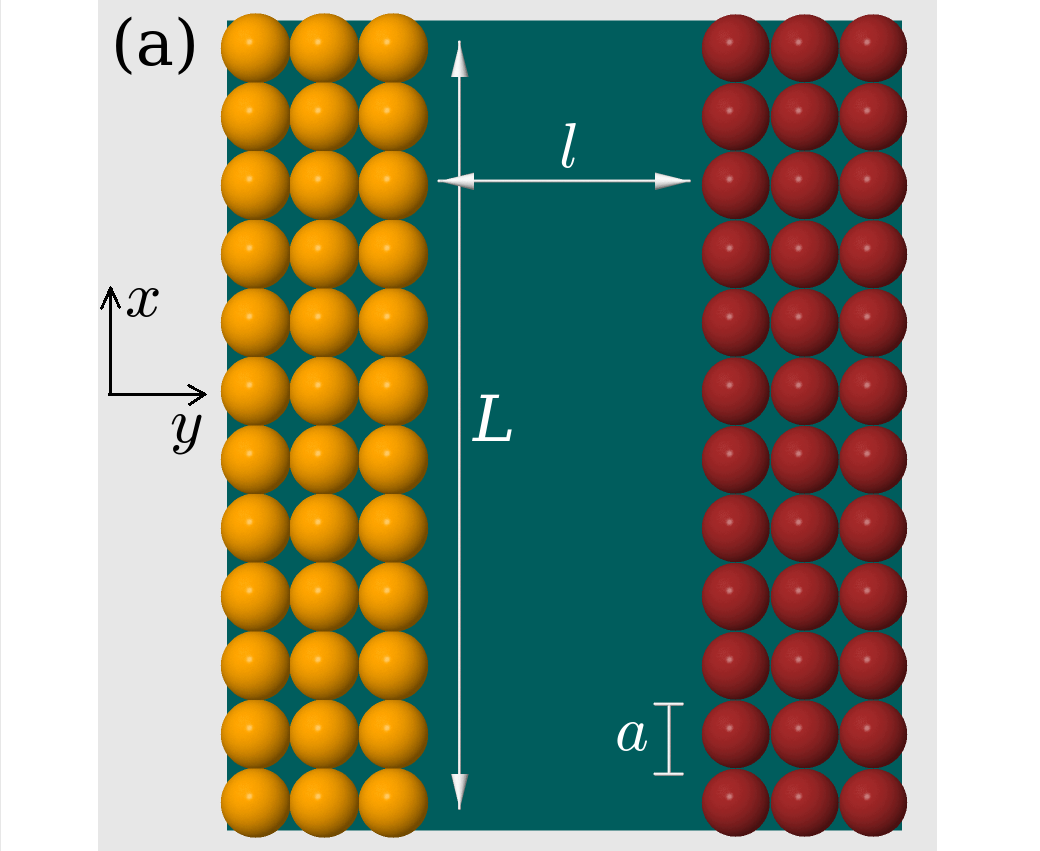
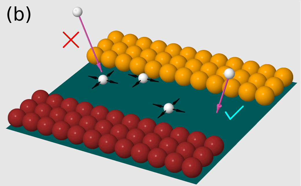
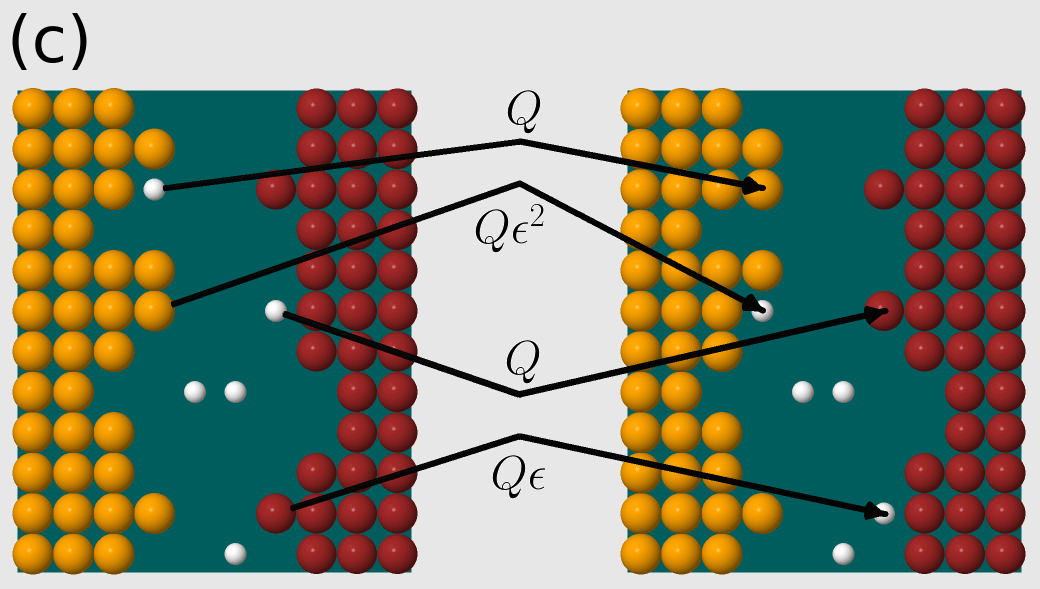
Figure 1: (a) Initial configuration of the grains A (yellow) and B (red). (b) Two particles incide at the gap (magenta arrows), the right one is accepted and the left one is rejected (excluded volume). Possible hops of particles already deposited in the gap are also indicated (black arrows). (c) Rates of the processes that bring the configuration at the left to the configuration at the right.

The external particle flux $F$ is the number of incident particles per site per unit time. If the incident particle reaches an empty site above the substrate, it becomes a mobile particle at that position; however, if it reaches an occupied site, the deposition attempt is rejected. This process is illustrated in Fig. 1(b).

The mobile particles can diffuse on the substrate, with a hopping rate to nearest neighbor (NN) sites per unit time equal to $D$. A hop attempt is executed only if the target site is empty, otherwise the mobile particle remains in the same position. The process is also illustrated in Fig. 1(b). The corresponding tracer diffusion coefficient is $Da^{2}/4$. The assumption that the excluded volume is the only type of interaction between mobile particles implies that other islands or grains are not formed in the gap.

The grains evolve via the attachment and detachment of particles. To facilitate the connection with kinetic roughening theory and other analytical approaches, these processes in each grain are restricted to the topmost point in each lateral coordinate $x$ (this is called the Solid-On-Solid constraint in the kMC and kinetic roughening literature). When a mobile particle is at the site immediately above the topmost grain particle, its attachment to the grain occurs with rate $Q$. Simultaneously, a topmost particle can detach from a grain with rate $Q\epsilon^{n}$, where $n$ is the number of NNs of that grain and $\epsilon<1$ is termed the detachment probability per NN. These processes are illustrated in Fig. 1(c). With these rules, the attachment rate does not depend on the local configuration of the grain edge. However, the detachment is facilitated at edge tips ($n=1$) and is more difficult at flat regions of the edges ($n=3$).

After the edge collision, the boundary between the grains A and B is formed. The above rules for attachment and detachment are maintained and the interactions between particles of different grains are restricted to excluded volume interactions. This means that the formation of bonds between NN particles of different grains is neglected. This may be a reasonable approximation if the actual inter-grain bonds of a material are sufficiently weak in comparison with the intra-grain bonds. In this approximation, the characteristic time scales of the grain edge dynamics are not much different before and after the collision.

The diffusion and detachment of particles are expected to be temperature activated processes, so that the rates $D$ and $\epsilon$ increase as the temperature increases. In many systems, the attachment is also activated, so $Q$ also increases with the temperature. These parameters may then be written in Arrhenius forms (see Sec. S.I of the Supplementary Material). It defines a true thermodynamic equilibrium in the model without deposition, which is enforced by detailed balance. However, since our aim is to address possible properties of several 2D materials, we do not choose a set of activation energies for the simulations, but study a large variety of possible relations between those rates and the flux $F$.

2.2 Simulations and quantities of interest

Simulations were performed in lattices with edge length $L$ varying from $128a$ to $1024a$; most results are obtained for $L=512a$. The initial gap width $l$ varies between $16a$ and $128a$. The model rates in the simulations are measured in terms of the flux rate $F$. The ratios $F/D$ and $F/Q$ vary from ${10}^{-8}$ to ${10}^{4}$; these limiting values respectively represent very low and very high fluxes for a given temperature. Most simulations are performed with $\epsilon=0.1$, which implies that the detachment rates have a weak dependence on the coordination number $n$; this is reasonable only at high temperatures for most materials ($k_{B}T\approx 0.43$ times the activation energy per NN). Additional simulations were performed with $0.01\leq\epsilon\leq 0.07$ to analyze the effects of this parameter.

For most parameter sets, average quantities are calculated over $100$ different configurations, but in some cases ${10}^{3}{\text{--}}2\times{10}^{3}$ configurations are considered. The kinetic Monte Carlo algorithm developed for these simulations is similar to that of previous works on submonolayer growth [32, 33, 34].

The main quantity calculated here is the roughness of the grain edges. Letting $h\left(x,t\right)$ to denote the height of an edge at position $x$ and time $t$ measured relatively to its initial position, the roughness is defined as

$$W\equiv{\langle\;{\overline{{\left(h-\overline{h}\right)}^{2}}}\;\rangle}^{1/2},$$ (1)

where the overbars denote a spatial average (over the values of $x$ in a given sample) and the angular brackets denote a configurational average (over different samples). Due to the symmetry of the grains A and B, our configurational average also includes averaging over the two grains of each growing sample.

We also measure the gap coverage, which is the fraction of the initial gap covered by deposited particles:

$$\theta=\frac{N_{d}}{\left(L/a\right)\left(l/a\right)},$$ (2)

where $N_{d}$ is the total number of deposited particles. Observe that particle attachment and detachment do not affect this quantity.

To characterize the transition from edge growth (when attachment dominates over detachment) to GB relaxation (when the grains evolve with balanced attachment and detachment), we define an average collision time $t_{c}$. For each position $x$ and a given configuration of evolving grains, the local collision time $t_{c}^{\left(local\right)}\left(x\right)$ is defined as the first time in which grains A and B occupy NN sites at position $x$ (with any value of $y$). Observe that the GB is not frozen after collision, so particles may detach from one of the grains, move to NN sites, or reattach to one of the two grains. The value of $t_{c}$ is obtained by averaging $t_{c}^{\left(local\right)}$ over all positions $x$ and over different configurations of evolving grains; this averaging also gives the standard deviation of the collision times, $\Delta t_{c}$.

3 Results and Discussion

3.1 Morphological evolution

Figs. 2(a)-(c) show snapshots of the deposits grown with different values of the incident flux but with constant values of $D$, $Q$, and $\epsilon$, which are set to $Q/D={10}^{-1}$ and $\epsilon=0.1$. This is expected to mimic constant temperature conditions with variable precursor fluxes. The growth times are shown in dimensionless units of $Dt$.

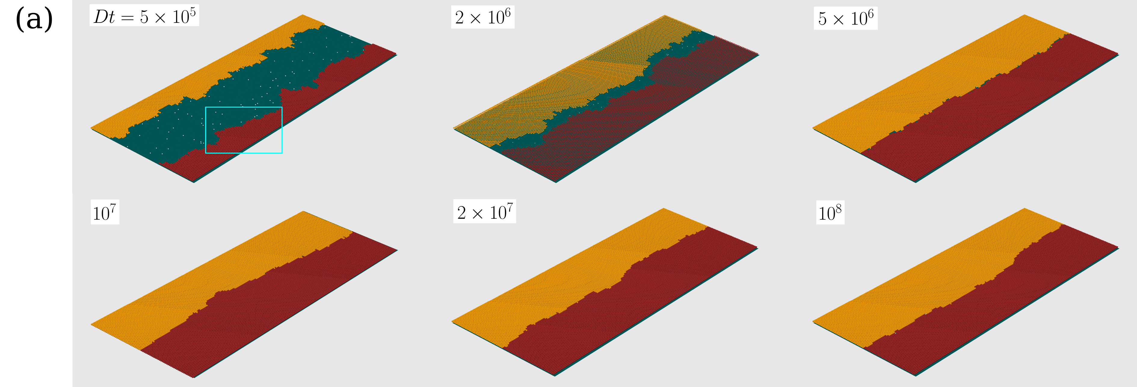
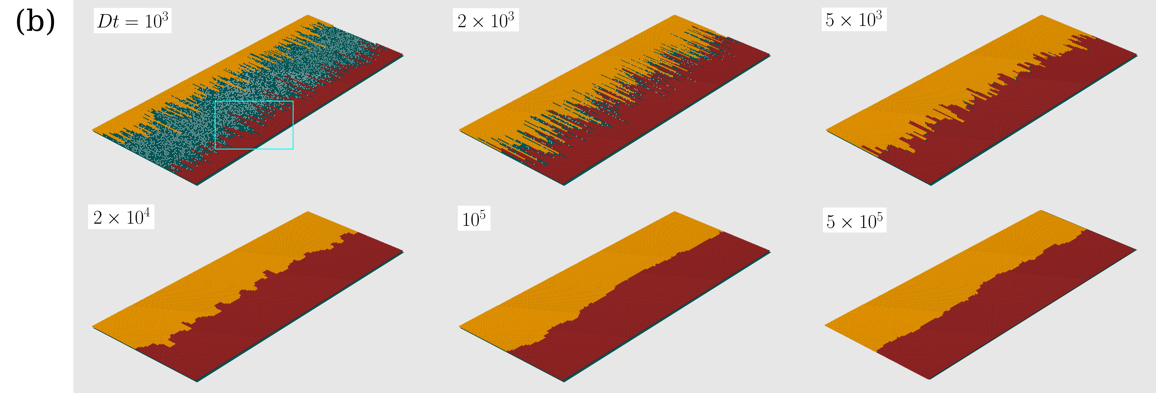
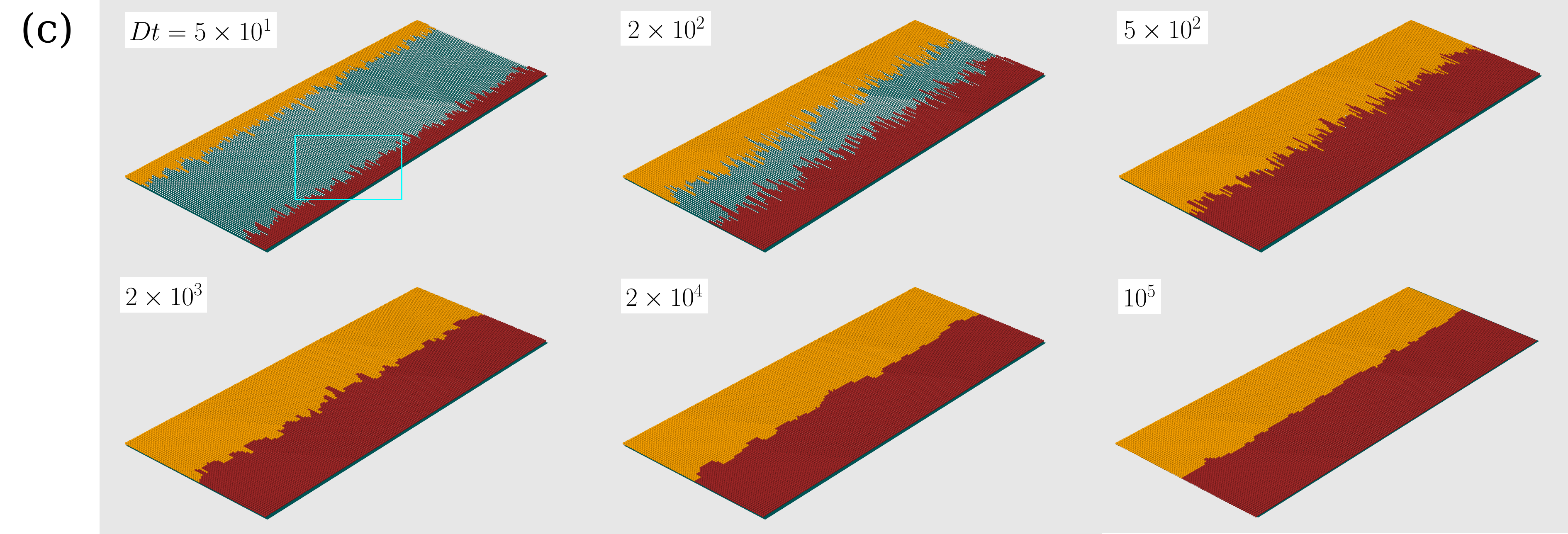
Figure 2: Snapshots of parts of the deposits grown with $Q/D={10}^{-1}$, $\epsilon=0.1$, $L=1024a$, and $l=128a$: (a) $F/D={10}^{-6}$; (b) $F/D={10}^{-3}$; (c) $F/D=10$. Light blue rectangles indicate the regions highlighted in Fig. 3.

For the lowest flux ($F/D={10}^{-6}$), Fig. 2(a) shows that the roughness of the growing edges is dominated by long wavelength fluctuations. The mounds and valleys evolve from typical sizes $10a{\text{--}}30a$ at $Dt=5\times{10}^{5}$ to sizes larger than $30a$ at $Dt=2\times{10}^{6}$, but no significant change in the edge roughness is visible. The particle density in the gap is very small until the grain collision; this is confirmed by the magnified view in Fig. 3(a) of the region highlighted in Fig. 2(a). Similar evolution is observed for larger diffusion coefficients of the particles in the gap, i.e. when $Q/D$ and $F/D$ decrease by the same factor, as shown in Sec. S.II of the Supplementary Material. These features are representative of the attachment limited growth regime in this model.

As the gap is closed and a GB is formed, there is a drastic decrease of the boundary roughness. This decrease is also observed in models of collisions of uncorrelated interfaces that propagate with finite velocities and is independent of the detailed physics of their short range interactions [35]. After the collision, the GB evolves slowly by detachment of particles from one edge followed by reattachment to the other, with apparently small changes in the roughness.

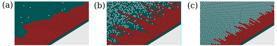
Figure 3: (a), (b), and (c) show zooms of the regions indicated in Figs. 2(a), 2(b), and 2(c), respectively.

For the intermediate value of the flux ($F/D={10}^{-3}$), but the same ratio $Q/D$, Fig. 2(b) shows spikes at the grain edges since early times. At $Dt={10}^{3}$, a high particle density is already present in the gap. note that this time is much shorter than that of the first panel of Fig. 2(a). The magnified view in Fig. 3(b) shows that the particle density is depleted only near the valleys of the grain edges. For this reason, the spikes grow faster than the valleys, as noticeable by comparing the snapshots at $Dt={10}^{3}$ and $2\times{10}^{3}$ in Fig. 2(b). This is characteristic of unstable growth in a diffusion-limited regime.

The spikes that result from the unstable growth are particular features of this model. They contrast with the fractal or dendritic shapes observed in experiments and in other models with unstable growth [3, 17]. This difference is a consequence of the condition that particle attachment occurs only at the topmost site at each $x$, which prevents the lateral attachment responsible for more complex morphologies.

When the gap is completely filled, the spikes remain, so the GB roughness is initially large. At $Dt=2\times{10}^{4}$, Fig. 2(b) shows that the spikes are transformed to shorter and thicker structures. A smooth GB is achieved at $Dt={10}^{5}$, which is a much shorter time than that of the attachment-limited mode shown in Fig. 2(a).

Fig. 2(c) shows results for much higher flux, $F/D=10$, again with the same $Q/D$. Now the particle attachment is very slow compared to the incoming flux. At a short time, $Dt=5\times{10}^{1}$, the gap is fully covered [see the magnified view in Fig. 3(c)] and so it remains until the two edges collide and form a GB. This contrasts with the diffusion-limited regime, in which the density was depleted near the edge valleys. In the present situation, the mobile particles are effectively static. The attachment to the grain edges is consequently uncorrelated since short times because all points of the edge (at valleys or crests) are in contact with one of those particles. Fig. 2(c) also shows edges with spikes, but they are thinner and less protuberant than those of the diffusion-limited regime [Fig. 2(b)].

The GB is formed at $Dt\sim{10}^{3}$ with a non-negligible roughness. The relaxation of the GB leads to its smoothening. This process is comparably faster than that reported in Fig. 2(b), although the only relevant parameters, $Q$ and $\epsilon$, are the same. Indeed, at $Dt=2\times{10}^{4}$, the surface roughness in Fig. 2(c) is much smaller than that observed in Fig. 2(b).

In Sec. S.II of the Supplementary Material, we show that similar morphologies are obtained if the ratio $Q/D$ decreases by a factor ${10}^{2}$, corresponding to a larger particle diffusivity. A full coverage of the gap is also attained at short times for a high value of the flux, which corresponds to the same ratio $F/Q={10}^{2}$ of Fig. 2(c).

Thus, an apparently different growth regime is observed when the precursor flux is sufficiently high to produce full surface coverage before a significant edge displacement. In this high coverage regime, the GB may have an initially large roughness, but it attains smooth configurations in shorter times than those observed in diffusion-limited and attachment-limited regimes.

3.2 Roughness, coverage, and edge collision time

Fig. 4(a) shows the time evolution of the roughness $W$ of the grain edges for $Q/D={10}^{-1}$, $\epsilon=0.1$, initial gap width $l=64a$, edge length $L=512a$, and several values of $F/D$. For most of the flux values, Fig. 4(a) also indicates the typical ranges of collision times, which indicate the GB formation. Fig. 4(b) shows the coverage $\theta$ as a function of time for the same parameter sets.

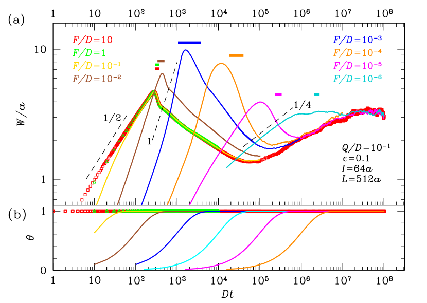
Figure 4: (a) Roughness evolution for constant $Q/D={10}^{-1}$ and variable flux. Dashed lines with the indicated slopes are drawn for comparison with the slopes of the plots. Horizontal bars at $W/a\lesssim 1$ indicate the edge collision times (average plus and minus one standard deviation). (b) Evolution of the gap coverage for the same parameter sets, with the same color code of (a).

In all cases, $W$ increases during edge growth, as expected for any kinetic roughening process starting from a flat configuration [36, 37]. In most cases, $W$ attains a maximal value near the average collision time (the only exception is the case with the lowest flux, in which $W$ seems to saturate after the initial increase). That result parallels the previous observation of a decrease of the roughness during the collision of interfaces propagating with constant velocities, independently of their short range interactions [35]. The smoothening or roughening processes that take place after the formation of the GB depend on the flux.

The lowest flux in Fig. 4(a), $F/D={10}^{-6}$, corresponds to the snapshots in Fig. 2(a). The plot shows that the initial near-equilibrium growth occurs with $W\sim t^{1/4}$. This is the roughening described by the Edwards-Wilkinson (EW) equation [38] at coarse grained scale, in which the surface tension and an uncorrelated noise are the main mechanisms. The relative fluctuation of the collision time is not large, as inferred by the width of the indicative bar in Fig. 4(a). After the GB formation, there are small changes in the roughness, which indicate that the GB attains a stationary regime.

The stationary regime can actually be mapped to a true thermodynamic equilibrium state, in which the roughness depends only on the detachment probability $\epsilon$ and on the edge length $L$; see details in Sec. S.III of the Supplementary Material. For all values of the model rates ($F$, $D$, and $Q$) and of the initial gap width, the roughness is expected to converge to the same stationary value at sufficiently long times. Thus, depending on the maximal roughness attained before the grain collision, $W$ may increase or decrease after formation of the GB. For instance, Fig. 4(a) shows that $W$ increases towards the stationary value for $F/D={10}^{-5}$ and $F/D={10}^{-4}$; however, Sec. S.IV of the Supplementary Material shows that $W$ decreases towards the stationary value when the gap width is smaller.

For the intermediate flux, $F/D={10}^{-3}$, Fig. 4(a) shows that the initial increase of the roughness is faster than linear; it corresponds to the snapshots in Fig. 2(b). The explosive increase of height fluctuations confirms the unstable growth which is expected in a diffusion-limited regime. The range of collision times is broader in this case, as a consequence of the large dispersion in the local heights of the two edges. When the edges collide, $W$ decreases and can reach much smaller values as the GB relaxes. After reaching a minimal value, $W$ increases again (it is expected to converge to the stationary value at long times). In previous studies of sudden changes from a first kinetics that produces faster roughening to a second kinetics that produces slower roughening, similar results were obtained, viz. rapid smoothening after the change and subsequent slow roughening [39, 40].

For the largest flux ($F/D=10$), the roughness in Fig. 4(a) approximately increases as $W\sim t^{1/2}$; the corresponding snapshots are in Fig. 2(c). This is consistent with random uncorrelated deposition at both grain edges [36]. Fig. 4(b) shows that full substrate coverage is attained long before the collision time, in contrast with the other regimes, in which the coverage is $1$ only at times near the collision. This confirms that the separated grain edges grow with a fully covered gap. The maximal $W$ is also attained as the edges collide and the subsequent decrease is associated with the GB formation. However, the range of collision times is small compared to the unstable regime. After the GB is formed, the roughness attains a minimum value which is smaller than the values obtained in the near-equilibrium and in the diffusion-limited regimes. Moreover, this mininum value is attained in a shorter time compared to those regimes, as previously suggested by the snapshots of Figs. 2(a)-(c).

A common feature of the regimes limited by attachment and by diffusion is that the time of GB formation (the average collision time) is roughly proportional to the reciprocal of the flux rate: $t_{c}\sim 3/F$. The initial gap width and the mechanisms of particle diffusion, attachment, and detachment determine the edge morphology. However, in the high coverage regime (obtained with the highest fluxes), the time of GB formation depends on the rate $Q$ but not on the flux $F$; for instance, compare the data for $F/D=1$ and $F/D=10$ in Fig. 4(a). After the gap is (rapidly) filled, the attachment rate $Q$ controls the edge propagation, with negligible effect of the diffusion rate because the particle positions are effectively frozen. Thus, the collision time is inversely proportional to $Q$ and proportional to the gap width $l$; see details in Sec. S.V of the Supplementary Material.

Between the three regimes described above, the roughness evolution shows crossover features. In Fig. 4(a), $F/D={10}^{-5}$ and ${10}^{-4}$ represent the crossover between the attachment-limited and the diffusion-limited regimes, whereas $F/D={10}^{-2}$ and ${10}^{-1}$ represent the crossover from the latter to the high coverage regime.

Qualitatively similar results are obtained for other ratios $Q/D$. Fig. 5(a) shows the roughness evolution for several values of the flux $F$ when $Q/D={10}^{3}$, which represents systems with very slow surface diffusion in comparison with the attachment and detachment rates; the other parameters remain the same as in Fig. 4(a) and the time scale of diffusion is also used for the data presentation. The main difference here is that the diffusion-limited (unstable) regime spans a broader range of $F$, since the slow diffusion favors the particle depletion near the edge valleys. For this reason, the attachment-limited regime is not observed in Fig. 5(a). However, or $F/D={10}^{4}$ (corresponding to $F/Q=10$), the features of the high coverage regime are also observed: the edges initially show the $W\sim t^{1/2}$ scaling of uncorrelated growth, while the coverage has already reached the full value $1$, as shown in Fig. 5(b); after the GB formation, $W$ reaches a minimal value smaller than those attained in the other regimes, and this occurs at a shorter time.

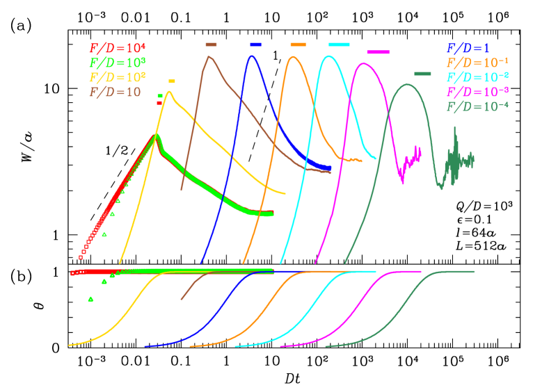
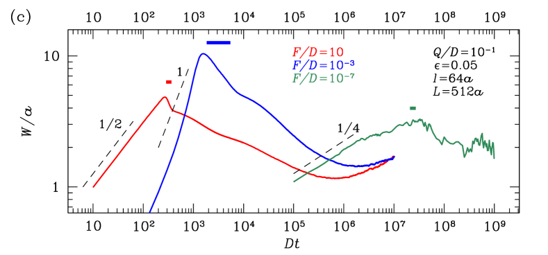
Figure 5: (a), (c) Roughness evolution for constant $Q/D$ and variable flux. Dashed lines with the indicated slopes are drawn for comparison with the slopes of the plots. Horizontal bars at $W/a\lesssim 1$ indicate the edge collision times (average plus and minus one standard deviation). (b) Coverage evolution for the same parameters in (a), with the same color code.

Much larger diffusion coefficients (compared to the attachment rate) facilitate the particle redistribution in the gap and permit the observation of the attachment-limited regime, but suppress the unstable regime (diffusion-limited). However, for the largest flux rates, the features of the high coverage regime are still observed because the diffusion is not effective in this case. This is illustrated in Sec. S.VI of the Supplementary Material for $Q/D={10}^{-3}$.

Changes in the gap width $l$ affect the crossover between the diffusion-limited and the attachment-limited regimes, but do not change the features of the very high flux regime. For smaller $l$, the unstable growth may not have sufficient time to develop, so the EW roughening of the edges is observed for slightly larger fluxes; see Sec. S.IV of the Supplementary Material. Instead, for larger $l$, the unstable regime extends to smaller fluxes because the instability has longer time to develop before the edges collide.

Changes in the detachment probability $\epsilon$ (which relates the detachment rates with the number of NNs) lead to some relevant changes in the roughness evolution, as shown in Fig. 5(c) for $\epsilon=0.05$ and the other parameters kept the same as in Fig. 4(a). First, a smaller $\epsilon$ pushes the diffusion-limited regime to lower fluxes because the detachment kinetics of the edges is slower, but the attachment does not change. For this reason, a clear EW scaling of the roughness is observed only for $F/D={10}^{-7}$ [in contrast with $F/D={10}^{-6}$ for $\epsilon=0.1$; Fig. 4(a) ]. Second, for the intermediate and the largest fluxes, the smaller detachment rates leads to slower decays of the roughness after the GB formation. Despíte these differences, the high coverage regime obtained with the highest flux ($F/D=10$) still provides the smallest GB roughness during the relaxation.

For the largest flux in Fig. 5(c) ($F/D=10$), a nontrivial feature is the appearance of shoulders in the decay of the GB roughness. The decrease of the roughness upon the collision is a stochastic effect characteristic of interface collisions [35]. After that, the roughness decreases by the elimination of the thinnest spikes of the GB, which requires the detachment of particles with $n=1$ NN, whose rate is $Q\epsilon$. For small $\epsilon$, this rate is much smaller than that of the initial growth ($Q$); the first shoulder is a consequence of the longer time scale associated to this process. Further relaxation of the GB depends on kink detachment (see Sec. S.III of the Supplementary Material), whose rate is $Q\epsilon^{2}$. This is smaller than the rate of spike elimination by the factor $\epsilon$, which explains the second shoulder. These features become more pronounced for smaller $\epsilon$, as shown in Sec. S.VII of the Supplementary Material; however, the high coverage regime still provides the minimal roughness in a shorter time than the other growth regimes.

3.3 Phase diagram of grain edge growth

In our simulations, we identify three regimes of edge growth, i.e. before the edges begin to interact. The attachment-limited or near-equilibrium regime is charaterized by slopes of the $\log{W}\times\log{\left(Dt\right)}$ plots near the EW value $1/4$. The diffusion-limited or unstable regime is characterized by slopes larger than $1$ at some time interval before the maximal $W$. Finally, the very high flux or random growth regime is characterized by slopes near $1/2$. Other behaviors are considered as crossovers. Fig. 6 shows the phase diagram obtained with these criteria for $\epsilon=0.1$ and gap widths $l=32a$ and $64a$. For 2D materials such as graphene or metal dichalcogenides, the lattice constant is $\sim 0.3$ nm, so those values correspond to widths $\sim 10{\text{--}}20$ nm.

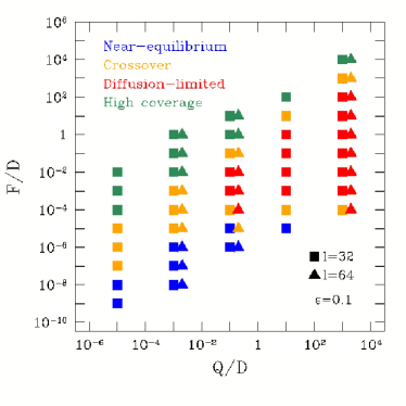
Figure 6: Grain growth regimes as function of the kinetic parameters for $\epsilon=0.1$ and two gap widths.

For very slow attachment-detachment kinetics in comparison with diffusion (very small $Q/D$), the unstable growth is not observed because the mobile particles are uniformly distributed in the gap. The unstable growth is typically observed for $F/Q\lesssim 0.1$ (to avoid the rapid uncorrelated growth), $F/D\gtrsim{10}^{-3}$ (to avoid very slow deposition, which favors near-equilibrium growth), and $Q/D\gtrsim 1$ (fast interface kinetics compared to diffusion).

However, these conditions change as the gap width $l$ or the detachment probability $\epsilon$ change. For wider gaps, the instability has longer time to develop before the edge collision, so it can be observed for smaller values of $F/D$. As $\epsilon$ decreases, particle detachment becomes slower, which also favors the instabilities; thus, the unstable regime can also be observed for smaller values of $F/D$.

The high coverage regime is more robust against changes in the physical or chemical parameters. It typically appears for $F/Q\gtrsim 10$, which is a condition in which the gap is almost completely filled before the attachment of a single layer of particles at each edge. As explained before, the diffusion coefficient $D$ is not important in this regime because the particles in the gap cannot move to the occupied NNs.

3.4 The minimal GB roughness

In the simulations of growth with high precursor coverage ($F/Q\gtrsim 10$), we measured the minimal value of the roughness obtained during the GB relaxation, $W_{min}$, and the time in which this minimum was attained, $t_{min}$.

$W_{min}$ does not depend on the parameters $F$, $Q$, $D$, and $L$; it is affected only by the detachment rate $\epsilon$ and the gap width $l$. Fig. 7(a) shows $W_{min}/a$ as a function of the scaling variable $\epsilon l/a$, i.e. the dimensionless product of the above parameters. Since the time of the minimal roughness rapidly increases as $\epsilon$ decreases and the simulations become slower as $l$ increases, we considered restricted ranges for those variables ($0.05\leq\epsilon\leq 0.1$ and $16\leq l\leq 64$) to obtain accurate estimates of $W_{min}$. The linear fit in Fig. 7(a) gives the relation

$$W_{min}\approx 0.87{\left(\epsilon a^{3}l\right)}^{0.25}.$$ (3)

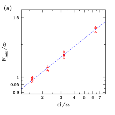
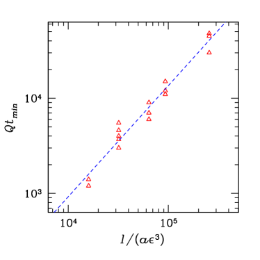
Figure 7: (a) Minimal roughness in the high coverage regime as a function of $\epsilon l/a$. The dashed line is a least squares fit with slope $0.25$. (b) Scaled time of the minimal roughness as a function of $l/\left(a\epsilon^{3}\right)$. The dashed line is a least squares fit with slope $0.16$.

The dependence of $W_{min}$ on $l$ can be explained by simple scaling arguments [39, 40]. From the initial flat edge condition to the edge collision, each of the grains is displaced by an average length $l/2$; thus, the average number of particles attached to each column $x$ of a grain is $N=(l/2)/a$. The uncorrelated growth in this regime leads to a maximal roughness of order [36]

$$W_{max}\sim a\sqrt{N}=\sqrt{\frac{al}{2}};$$ (4)

the characteristic rate of this growth is $Q$. As the GB is formed, there is a sudden change from this uncorrelated growth to a correlated kinetics. If the characteristic rate of attachment and detachment of the final kinetics is the same as the initial one, the uncorrelated fluctuations are rapidly suppressed and the roughness rapidly reaches the same time evolution of the final kinetics starting from a flat interface (see e.g. Fig. 6 of Ref. [39]); here, this would be the case of $\epsilon\sim 1$. The GB kinetics is EW (Sec. S.III of the Supplementary Material), in which the growth from a flat interface leads to $W\sim aN^{1/4}$, where a prefactor of order $1$ is excluded [38, 36]. The minimal roughness is then obtained by substituting the value of $N$ at the collision time in this relation, which gives $W_{min}\sim l^{1/4}$.

However, to describe the GB relaxation with smaller $\epsilon$, a more powerful approach has to be used. We developed a Langevin model [41] which assumes that the GB evolution is controlled by kink site detachment from one grain (with characteristic rate $Q\epsilon^{2}$) and attachment to the other grain. In Sec. S.III of the Supplementary Material, this model is solved for an initial surface configuration with uncorrelated roughness $W_{max}$ and predicts

$$W_{min}^{\left(\text{Lang}\right)}={\left[\frac{1}{\pi(1-\epsilon)^{2}}\right]}^{1/4}{\left(a^{3}l\epsilon\right)}^{1/4}.$$ (5)

Since $1-\epsilon\approx 1$ is a reasonable approximation in our simulations, Eq. (5) leads to the same scaling in $l$ and $\epsilon$ of Eq. (3); the approximation gives a prefactor $0.75$, which is not distant from the numerical estimate $0.87$ in Eq. (3).

The Langevin approach also predicts that the minimum roughness is attained at

$$t_{min}^{\left(\text{Lang}\right)}=\frac{l}{2aQ}\left[1+\frac{(1-\epsilon^{2})}{8\epsilon^{3}}\right],$$ (6)

where the first term accounts for the uncorrelated growth of the edges of independent grains and the second one accounts for the coarsening of the GB. For $\epsilon\ll 1$, the first term is negligible in comparison with the second one, which gives $t_{min}^{\left(\text{Lang}\right)}\approx l/\left(16aQ\epsilon^{3}\right)$; this is expected to be a reasonable approximation even for $\epsilon=0.1$, which was considered in most simulations. Guided by this analytical result, Fig. 7(b) shows $Qt_{min}$ as a function of $l/\left(a\epsilon^{3}\right)$, which reasonably fits a straight line. The slope of that fit is $0.16$, which is larger than, but of the same order of the theoretical slope $1/16$.

3.5 Possible application to 2D materials growth

Here we discuss the application of the growth in the high coverage regime to produce 2D materials with small GB roughness.

Eqs. (3) and (5) show that decreasing the growth temperature (so that $\epsilon$ decreases) is advantageous for obtaining a smaller GB roughness. However, Eq. (6) shows that it is disadvantageous for increasing the time to attain this minimal roughness because $Q$ and $\epsilon$ decrease. Evidence on this disadvantage is provided by the comparison of Figs. 4(a) ($\epsilon=0.1$) and 4(c) ($\epsilon=0.05$) with Fig. S.6 of the Supplementary Material ($\epsilon=0.01$). The advantage involves a factor $\epsilon^{1/4}$ and the disadvantage involves a factor $1/\left(Q\epsilon^{3}\right)$, so we generally expect that higher temperatures will be more favorable for obtaining smoother GBs. This implies that $\epsilon$ and $Q$ are large. However, the condition $F/Q\gtrsim 10$ is also necessary to allow the initial uncorrelated growth of the separated grain edges (Sec. 3.3).

For the application to a particular 2D material, it is necessary that isolated grains nucleate and grow to a configuration with smooth boundaries, which is the initial condition considered here; observe that the formation of this initial configuration is not addressed by our model. In such configuration, a common situation is that the grains cover a fraction of the substrate $\lesssim 0.1$. The inspection of microscopy images with visible and isolated islands (grains) of 2D materials supports this estimate [1, 42, 43, 44, 45, 46]. Instead, with coverages $\sim 1$, coalescence of several islands may be observed. Thus, if the separated grains have typical boundary length $L$, the gap width $l$ is expected to be of a similar order of magnitude; for simplicity, the approximation $l\approx L$ is considered here.

Following the reasoning in the paragraphs above, we also assume that: edge lengths $L$ and initial gap widths $l$ are $\sim 10\mu{\text{m}}$; the lattice constant of the material is $a\approx 0.3$ nm (which differs $\lesssim 20\%$ from graphene and several metal dichalcogenides); $\epsilon=0.1$, meaning kink detachment rate $10^{2}$ times smaller than the attachment rate; the condition $F/Q\leq 10$ is fulfilled.

From Eq. (4), the maximal roughness of the grain edges in these conditions is $\sim 40$ nm. However, Eq. (3) predicts that the minimal roughness attained by the GB is $\sim 2$ nm, corresponding to a decrease by a factor $\sim 20$. The time to attain the minimal roughness can be determined from Eq. (6) in terms of the attachment rate: $Qt_{min}\sim 4\times{10}^{6}$.

For comparison, if near-equilibrium growth conditions are chosen and the GB relaxes to its equilibrium configuration, the approach of Sec. S.III of the Supplementary Material predicts the GB roughness

$$W_{eq}=\sqrt{\frac{\epsilon aL}{6}}\left(\frac{1}{1-\epsilon}\right).$$ (7)

With the above parameters, we obtain $W_{eq}\sim 7$ nm, which is $3.5$ times larger than the expected minimal roughness. The time of crossover to the equilibrium roughness is obtained from the EW kinetics of the GB in Sec. S.III of the Supplementary Material:

$$Qt_{eq}=\frac{\pi}{144}{\left(\frac{L}{a}\right)}^{2}\frac{1}{\epsilon^{2}}\left(\frac{1+\epsilon}{1-\epsilon}\right).$$ (8)

It gives $Qt_{eq}\sim 3\times{10}^{9}$, which exceeds by three orders of magnitude the time to obtain the minimal roughness in the high coverage regime.

This comparison clearly shows that the advantages of growing 2d materials in the high coverage regime can be extrapolated from our nanoscale simulations to more typical experimental conditions with microscale grains. The decrease of the GB roughness up to the minimum can be observed in a much shorter time than that necessary for the GB to reach its equilibrium value, which is larger than that minimum.

Our model has the limitation that the mobile particle attachment is restricted to the topmost point of each column $x$. We noted that leads to unstable patterns that look very different from those of experiments and of models for specific applications. However, we believe that this limitation does not have significant effect on our prediction of a minimal roughness for the high coverage regime. If that condition for the attachment is relaxed, then the aggregation of mobile particles to the sides of the rough edges may lead to overhang formation. Such overhangs will encapsulate mobile particles, but these particles are effectively static in the high coverage condition. Thus, these particles will eventually attach at the same position and fill the overhang. It is possible that this process creates some lateral correlations along the edges, but such fluctuations, which are correlated at very small scales, can be suppressed approximately in the same way as the totally uncorrelated fluctuations considered here.

4 Conclusion

A model for the propagation of two grain edges of a 2d material and for the relaxation of the grain boundary formed after the collision of those edges was proposed. The model considers simple kinetic rules for attachment and detachment of particles from the edges and for particle diffusion while there is a gap between them. This allowed to perform kinetic Monte Carlo (KMC) simulations for broad ranges of model parameters and investigate their consequences on the geometry of the grain edges.

Besides the well known near-equilibrium (attachment-limited) and unstable (diffusion-limited) growth regimes, we observe the existence of a distinct third regime when the precursor flux is sufficiently high to fully cover the gap between the edges before they begin to grow. In this high covered regime, an uncorrelated growth of the edges is observed until they collide. Although this may produce an initial grain boundary with large roughness, we show that this boundary relaxes to configurations with a roughness smaller than those of the other regimes in a shorter time. Numerical predictions of the minimal roughness and of the time to attain such configuration are in good agreement with a theoretical approach for the grain boundary relaxation of the model.

To investigate the possible extension of the above results to real grains of 2d materials, the simulation results (obtained at nanoscale) were extrapolated to edges and gaps sizes $\sim 10\mu{\text{m}}$. It shows that the high coverage regime can produce grain boundaries with minimal roughness $\sim 2$ nm, which is $\sim 3.5$ times smaller than the roughness obtained in a near-equilibrium, stationary state. Moreover, the time to obtain that minimal roughness is three orders of magnitude smaller than the expected time for the grain boundary to reach that stationary state. Thus, if the control of the growth conditions of a 2d material permits to reach an initial high coverage condition and a relaxation dynamics as proposed here, it is possible that a novel route for efficient growth of that material with very smooth grain boundaries can be developed. Recent advances in microscopy methods allow accurate measurements of nanoscale fluctuations of GBs and may help such studies [47, 48].

Supplementary Material

The Supplementary Material shows the possible temperature dependences of the model parameters, additional images of the evolution of the grain boundaries, additional plots of the roughness evolution, the Langevin model for grain boundary dynamics, and the scaling of collision times in near-equilibrium and unstable regimes.

S.I Temperature dependence of model parameters

The diffusion coefficient of particles that are not bonded to the grains can be written as

$$D=a^{2}\nu\exp{\left(-E_{s}/k_{B}T\right)}$$ (S1)

where $\nu$ is a frequency, $E_{s}$ is an activation energy, $k_{B}$ is the Boltzmann constant and $T$ is the temperature. In the deposition model of Clarke and Vvedensky [49], $\nu$ is proportional to the temperature. However, several simulation works consider a constant value $\nu\sim{10}^{12}{\text{s}}^{-1}$ and, under this assumption, obtain results in good agreement with experiments on deposition of metals and semiconductors [27]. Typical values of $E_{s}$ for those materials are on the orders $0.1{\text{--}}1$ eV.

The attachment rate of particles at the edge borders may be written as

$$Q=Q_{0}\exp{\left(-E_{a}/k_{B}T\right)}$$ (S2)

where $Q_{0}$ is an attempt frequency and $E_{a}$ is the activation energy for that process. These values are strongly dependent on the type of interaction between the atoms or molecules of the growing material. In some cases, $Q$ may be considered as temperature independent, so $E_{a}=0$; this is the case of several models of deposition of metal and semiconductor films [27].

The detachment probability can be written as

$$\epsilon=\exp{\left(-J/k_{B}T\right)},$$ (S3)

where $J$ denotes the bond energy with a NN.

S.II Morphological evolution with $Q/D={10}^{-3}$

Fig. S1(a) shows snapshots of parts of the deposits grown with $F/D={10}^{-8}$, $Q/D={10}^{-3}$, $\epsilon=0.1$, $l=64a$, and $L=1024a$. In this parameter set, the value of $D$ is ${10}^{2}$ times larger than that of Fig. 2a of the main text, with the other parameters kept at the same values. It is an example of edge growth in the attachment-limited regime.

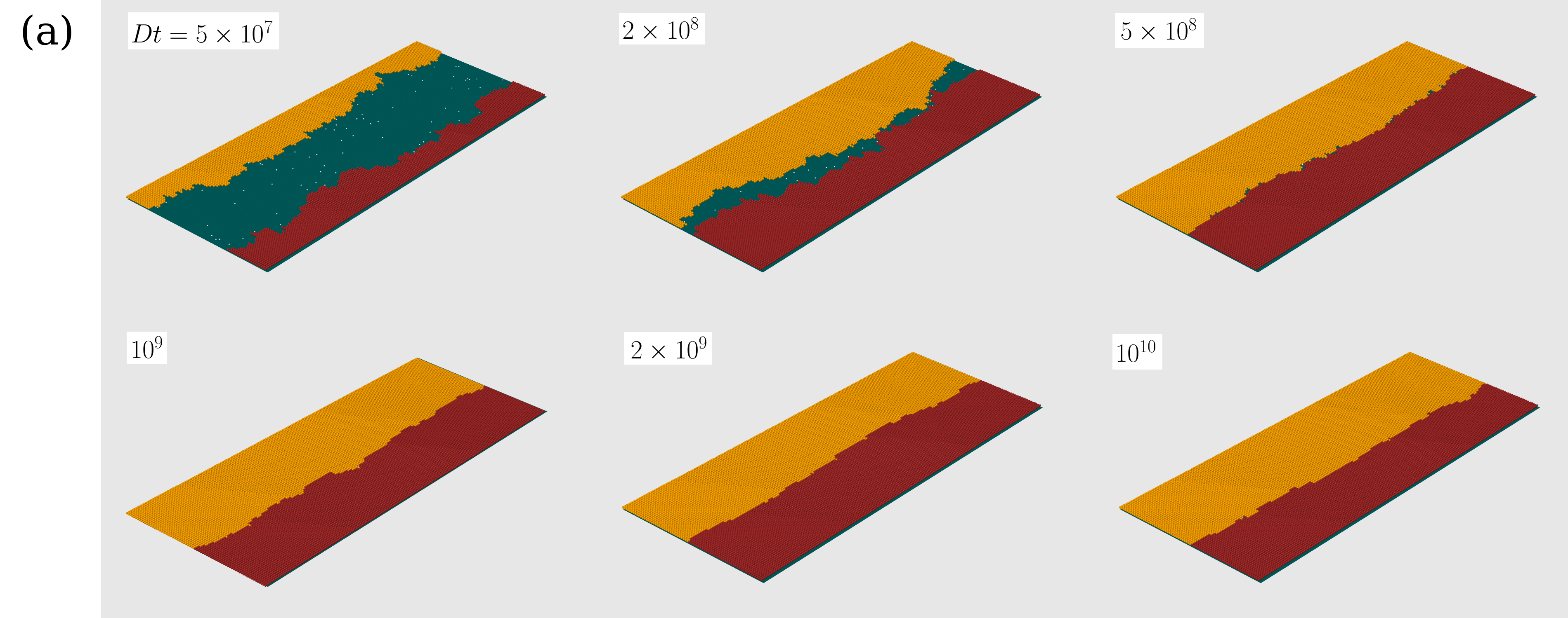
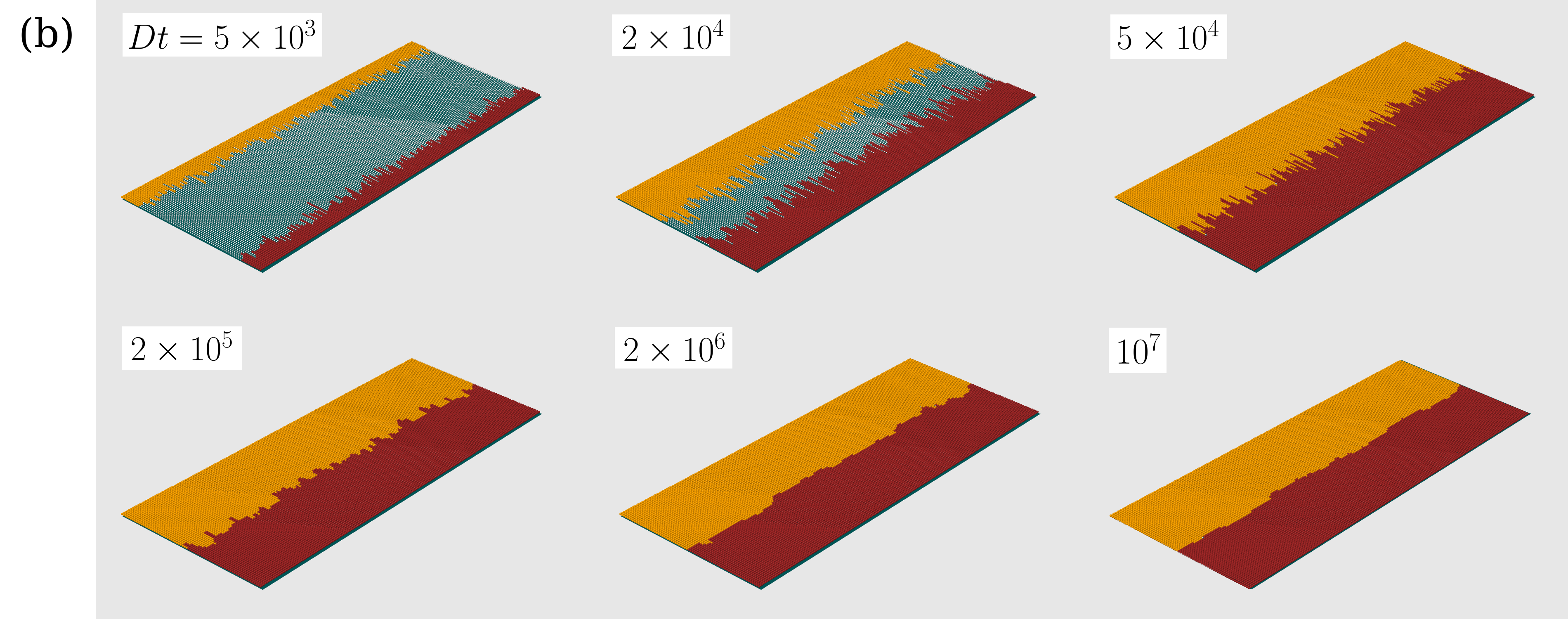
Figure S1: Snapshots of parts of the deposits grown with $Q/D={10}^{-3}$, $\epsilon=0.1$, $L=1024$, and $l=128$: (a) $F/D={10}^{-8}$; (b) $F/D={10}^{-1}$.

Fig. S1(b) shows snapshots of the deposits grown with $F/D={10}^{-1}$, $Q/D={10}^{-3}$, $\epsilon=0.1$, $l=64$, and $L=1024$. The value of $D$ is ${10}^{2}$ times larger than that of Fig. 2c of the main text, with the other parameters kept at the same values. It is an example of edge growth in the high coverage regime.

S.III Langevin model for GB dynamics

In this section, we propose a Langevin model for the dynamics of the GB, when all sites are occupied by atoms from the two grains. The dynamics is well described by two types of rates. The first one accounts for the rate $R_{+}$ at which an atom detaches from the upper crystal and reattaches to the lower crystal. Since the detachment rate is $\epsilon^{4-n}$ where $n$ is the number of in-plane nearest neighbors with the lower crystal, and the attachment rate is $Q/2$, we have

$$R_{+}(n) =\frac{Q}{2}\epsilon^{4-n}.$$ (S4)

Similarly, the rate of detachment from the lower crystal and attachment to the upper crystal is

$$R_{-}(n) =\frac{Q}{2}\epsilon^{n}.$$ (S5)

S.III.1 Derivation from Einstein’s relation

Since atomic steps are 1D systems with short range interactions, they are always in a high-temperature phase, i.e., they are always rough and cannot undergo a low-temperature facetting transition. Hence, there is always a finite concentration of kinks. At low temperatures, their concentration is small and is given by the Boltzmann weight of non-interacting excitations of energy $E_{k}$. This leads to $p_{k}=2\exp[-E_{k}/k_{B}T]$, where $E_{k}=J$ is the kink energy, and the factor $2$ comes from the existence of two types of kinks (up and down kinks when going along $+x$).

Using a model with kinks of arbitrary heights (but imposing the SOS constraint that neglects the possibility of overhangs as in KMC) the kink density reads [26]

$$p_{k}=\langle|n|\rangle=\frac{2\mathrm{e}^{-J/k_{B}T}}{1-\mathrm{e}^{-2J/k_{B}T}}=\frac{2\epsilon}{1-\epsilon^{2}}\,.$$ (S6)

In addition, the hopping rate of a kink to the left or to the right is $R_{+}(2)=R_{-}(2)=R(2)$, so that the diffusion constant of a kink along the $x$ axis parallel to the (10) direction is

$$D_{k}=a_{\parallel}^{2}R(2)=a_{\parallel}^{2}\frac{Q}{2}\epsilon^{2}\,,$$ (S7)

where we have defined the lattice parameter $a_{\parallel}$ parallel to the GB ($a_{\parallel}=a$ in our simulations). From Einstein’s relation, the mobility of a kink is

$$M_{k}=\frac{D_{k}}{k_{B}T}=\frac{a_{\parallel}^{2}R(2)}{k_{B}T}\,.$$ (S8)

In the presence of a kink chemical potential $\mu_{k}$, the velocity of a kink is assumed to obey a linear kinetic law

$$v_{k}=-M_{k}\frac{\mu_{k}}{a_{\parallel}}\,.$$ (S9)

We now wish to make link with macroscopic quantities. The macroscopic position of the GB is $h_{GB}(x,t)$. Its macroscopic velocity   then reads [50, 51]

$$\partial_{t}h_{GB}=a_{\perp}\langle v_{k}\rangle\frac{p_{k}}{a_{\parallel}},$$ (S15)

where $a_{\perp}$ is the lattice constant in the direction perperdicular to the GB. Note that Eq.(S15) was derived in Refs.[50, 51] under the assumption that all kinks have the same velocity during growth. However, this relation is also valid at equilibrium where the motion of kinks is of the diffusion type with zero average. The relation between these two approaches is an example of the usual Einstein close-to equilibrium link between mobility for macroscopic motion under under fixed external force and diffusion at equilibrium.

Since $M_{k}$ does not vary from one kink to the other, we have [28]

$$\langle v_{k}\rangle=-M_{k}\frac{\langle\mu_{k}\rangle}{a_{\parallel}}$$ (S16)

and, since the chemical potential represents the free energy gain upon the addition of a single particle, we expect that the microscopic kink chemical potential and the macroscopic chemical potential to be equal:

$$\langle\mu_{k}\rangle=\mu.$$ (S17)

In addition, we use the standard macroscopic law

$$\mu=\frac{\delta{\cal F}/\delta h_{GB}}{\delta{\cal N}/\delta h_{GB}}=\Omega\tilde{\gamma}_{GB}\kappa\approx-\Omega\tilde{\gamma}_{GB}\partial_{xx}h_{GB}\,,$$ (S18)

where: ${\cal F}$ and ${\cal N}$ are respectively the edge free energy and the number of atoms in the lower crystal; $\Omega=a_{\parallel}a_{\perp}$ is the atomic area; $\tilde{\gamma}_{GB}$ is the grain boundary stiffness, obtained by the substitution $J\rightarrow 2J$ into the usual expression of the stiffness of a lattice model with bond energy $J$ (see, e.g. Ref. [26]), leading to:

$$\tilde{\gamma}_{GB}=\frac{k_{B}Ta_{\parallel}}{2a_{\perp}^{2}}\big{(}\varepsilon^{-1/2}-\varepsilon^{1/2}\big{)}^{2}.$$ (S19)

Finally, we obtain

$$\partial_{t}h_{GB}=-\frac{a_{\perp}}{a_{\parallel}}\frac{M_{k}\mu}{a_{\parallel}}p_{k}=\frac{R(2)p_{k}}{k_{B}T}a_{\perp}\Omega\tilde{\gamma}_{GB}\partial_{xx}h_{GB}\,.$$ (S20)

Adding a Langevin force $\eta_{GB}$, we obtain an EW equation

$$\partial_{t}h_{GB}=R(2)p_{k}a_{\perp}\Gamma_{GB}\partial_{xx}h_{GB}+\eta_{GB},$$ (S21)

with $\Gamma_{GB}=\Omega\tilde{\gamma}_{GB}/\left(k_{B}T\right)$. Using again the fluctuation dissipation theorem to determine the amplitude of the equilibrium Langevin force $\eta(x,t)$ (following the same lines as in Refs. [41, 28]), we obtain the roughness of the GB as

$$W_{GB}^{2} =\frac{2}{L^{2}}\sum_{n>0}\langle|h_{q}(0)|^{2}\rangle{\rm e}^{-2R(2)p_{k}a_{\perp}\Gamma_{GB}q^{2}t}$$

$$+\frac{L\Omega}{2\pi^{2}\Gamma_{GB}}\sum_{n>0}\frac{1}{n^{2}}\left(1-{\rm e}^{-2R(2)p_{k}a_{\perp}\Gamma_{GB}q^{2}t}\right),$$ (S22)

where $h_{q}\left(t\right)$ denotes the Fourier mode with $q=2n\pi/L$. At long times, we recover the well known expression of the equilibrium (stationary) roughness [26, 28]

$$W_{eq}^{2}=\frac{\Omega L}{12\Gamma_{GB}}\,,$$ (S23)

and using Eq.(S19) we obtain

$$W_{eq}^{2}=\frac{La_{\perp}^{2}}{6a_{\parallel}}\,\frac{\epsilon}{(1-\epsilon)^{2}}\,.$$ (S24)

At short times, we find

$$W_{GB}^{2} =\frac{2}{L^{2}}\sum_{n>0}\langle|h_{q}(0)|^{2}\rangle{\rm e}^{-2R(2)p_{k}a_{\perp}\Gamma_{GB}q^{2}t}$$

$$+\Omega\left(\frac{2R(2)p_{k}a_{\perp}}{\pi\Gamma_{GB}}t\right)^{1/2}\,.$$ (S25)

The second term of this equation is the well known equilibrium EW scaling. It is e.g. in agreement with Eqs.(2.63,2.65) of Ref. [28] with the substitution $(\nu_{+}+\nu_{-})\Omega c_{eq}^{0}\rightarrow R(2)p_{k}a_{\perp}$.

We substitute the expressions of $p_{k}$ and $\tilde{\gamma}_{GB}$ as a function of $\epsilon$ and obtain

$$W_{GB}^{2} =\frac{2}{L^{2}}\sum_{n>0}\langle|h_{q}(0)|^{2}\rangle{\rm e}^{-2R(2)p_{k}a_{\perp}\Gamma_{GB}q^{2}t}$$

$$+\Omega\left(\frac{4\epsilon^{4}a_{\perp}^{2}}{\pi(1+\epsilon)(1-\epsilon)^{3}a_{\parallel}^{2}}Qt\right)^{1/2}\,.$$ (S26)

S.III.2 Minimal roughness for fast growth with coverage $\theta=1$

The roughness in Eq. (S25) can exhibit a minimum. We re-write this equation as

$$W_{GB}^{2} =\frac{2}{L^{2}}\sum_{n>0}\langle|h_{q}(0)|^{2}\rangle{\rm e}^{-bn^{2}t}+\frac{L\Omega}{2\pi\Gamma_{GB}}\left(\frac{bt}{\pi}\right)^{1/2}\,,$$ (S27)

where

$$b =2R(2)p_{k}a_{\perp}\Gamma_{GB}\left(\frac{2\pi}{L}\right)^{2}\,.$$ (S28)

The evolution of $W_{GB}^{2}$ depends on the details of the initial condition which dictates the power spectrum $\langle|h_{q}(0)|^{2}\rangle$ just after collision.

In the limit of fast growth with coverage $1$, we assume that the growth regime before collision corresponds to RD, with forward atomic moves of the two interfaces appearing with a frequency $Q$. This gives a collision time $t_{0}=l/(2a_{\perp}Q)$ and a roughness before collision $W_{1bc}^{2}=a_{\perp}^{2}Qt_{0}=a_{\perp}l/2$. As discussed in Ref. [35], the collision reduces the square roughness by a factor $2$, so that after the collision $W^{2}_{1ac}=W_{1bc}^{2}/2=a_{\perp}l/4$. In the RD regime, the roughness is spatially uncorrelated, so

$$\langle h_{ac}(x)h_{ac}(x^{\prime})\rangle=W_{1ac}^{2}a_{\parallel}\;\delta(x-x^{\prime})$$ (S29)

and, in Fourier space,

$$\langle h_{ac,q}h_{ac,q^{\prime}}\rangle=a_{\parallel}W_{1ac}^{2}\;2\pi\delta(q-q^{\prime})=a_{\parallel}W_{1ac}^{2}\;L\delta_{n+n^{\prime}}\,.$$ (S30)

As a consequence, $\langle|h_{q}(0)|^{2}\rangle=a_{\parallel}W_{1ac}^{2}\;L={\Omega}lL/4$ in Eq.(S27), leading to

$$W_{GB}^{2} =\frac{2a_{\parallel}W_{1ac}^{2}}{L}\sum_{n>0}{\rm e}^{-bn^{2}t}+\frac{L\Omega}{2\pi\Gamma_{GB}}\left(\frac{bt}{\pi}\right)^{1/2}$$

$$=\frac{2a_{\parallel}W_{1ac}^{2}}{L}\Theta_{3}({\rm e}^{-bt})+\frac{L\Omega}{2\pi\Gamma_{GB}}\left(\frac{bt}{\pi}\right)^{1/2}\,,$$ (S31)

where $\Theta_{3}$ is the Elliptic Theta function. For $t\gg 1/b$, we have ${\rm e}^{-bt}\ll 1$, $\Theta_{3}({\rm e}^{-bt})\approx{\rm e}^{-bt}$, and

$$W_{GB}^{2} =\frac{2a_{\parallel}W_{1ac}^{2}}{L}{\rm e}^{-bt}+\frac{L\Omega}{2\pi\Gamma_{GB}}\left(\frac{bt}{\pi}\right)^{1/2}\,,$$ (S32)

i.e., the sum is dominated by the slowest decaying mode $n=1$. This expression does not necessarily lead to a minimum; the condition of existence of a minimum of the function ${\rm e}^{-x}+\alpha x^{1/2}$ is that $\alpha<2^{1/2}{\rm e}^{-1/2}$. Using $x=bt$, we obtain the condition for the presence of a minimum

$$\alpha =\frac{L^{2}\Omega}{4\pi^{3/2}W_{1ac}^{2}\Gamma_{GB}a_{\parallel}}<2^{1/2}{\rm e}^{-1/2}\,,$$ (S33)

which is re-written using the relation $W^{2}_{1ac}=a_{\perp}l/4$ as

$$L<L_{\mathrm{sup}} =\left(\frac{2\pi^{3}}{\mathrm{e}}\right)^{1/4}(l\Gamma_{GB})^{1/2}$$ (S34)

$$=\left(\frac{\pi^{3}}{2\mathrm{e}}\right)^{1/4}\left(\frac{l}{a_{\perp}}\frac{(1-\epsilon)^{2}}{\epsilon}\right)^{1/2}a_{\parallel}\,.$$

In the opposite regime $bt\ll 1$, when the time is to short to allow for the relaxation of the modes with wavelength close to the system size $L$, but long enough for short wavelength modes to have decayed (so that the sum on $n$ can be taken up to infinity), one can take the continuum limit in $n$:

$$\sum_{n>0}{\rm e}^{-bn^{2}t}\approx\int_{0}^{\infty}\mathrm{d}n\;{\rm e}^{-bn^{2}t}=\frac{1}{2}\left(\frac{\pi}{bt}\right)^{1/2}$$ (S35)

up to an additive constant related to the accuracy of the continuum limit around $n=0$. This leads to

$$W_{GB}^{2} =\frac{a_{\parallel}W^{2}_{1ac}}{L}\left(\frac{\pi}{bt}\right)^{1/2}+\frac{L\Omega}{2\pi\Gamma_{GB}}\left(\frac{bt}{\pi}\right)^{1/2}$$

$$=\frac{a_{\parallel}W^{2}_{1ac}}{\tau^{1/2}}+\frac{\Omega\tau^{1/2}}{2\pi\Gamma_{GB}}\,,$$ (S36)

where $\tau=L^{2}bt/\pi$.

A minimum then is found for $\tau_{min}=2\pi\Gamma_{GB}W_{1ac}^{2}a_{\parallel}/\Omega$, leading to

$$t_{min} =\frac{W_{1ac}^{2}}{4R(2)p_{k}a_{\perp}^{2}}=\frac{l}{16R(2)p_{k}a_{\perp}}\,.$$ (S37)

Interestingly, $t_{min}$ does not depend on the stiffness $\tilde{\gamma}_{GB}$. This minimum is obtained for $bt_{min}=2\pi^{2}a_{\parallel}\Gamma_{GB}W_{1ac}^{2}/(L^{2}\Omega)=\pi^{2}\Gamma_{GB}l/\left(2L^{2}\right)\ll 1$, leading to the condition

$$L>L_{\mathrm{inf}}=\pi(\Gamma_{GB}l/2)^{1/2}.$$ (S38)

Note the close similarity between the expressions of $L_{\mathrm{inf}}$ in Eq.(S38) and $L_{\mathrm{sup}}$ in Eq.(S34), which are identical up to their prefactors [which are numerically similar: $\pi\approx 3.14$ and $(8\pi^{3}/\mathrm{e})^{1/4}\approx 3.09$]. The value of the roughness at the minimum is

$$W_{min}^{2} =\frac{2W_{1ac}(a_{\parallel}\Omega)^{1/2}}{(2\pi\Gamma_{GB})^{1/2}}=\Omega\left(\frac{l}{2\pi\Gamma_{GB}}\right)^{1/2}$$ (S39)

$$=\frac{\Omega}{1-\epsilon}\left(\frac{\epsilon la_{\perp}}{\pi a_{\parallel}^{2}}\right)^{1/2}=\left(\frac{\epsilon a_{\perp}^{3}}{\pi(1-\epsilon)^{2}}\right)^{1/2}l^{1/2}\,.$$ (S40)

As a remark, $W_{min}^{2}$ does not depend on the kinetic coefficient $R(2)$.

Finally, the total physical time for the minimum is

$$t_{M} =t_{0}+t_{min}=\frac{l}{2a_{\perp}Q}\left(1+\frac{1}{4\epsilon^{2}p_{k}}\right)$$

$$=\frac{l}{2a_{\perp}Q}\left(1+\frac{(1-\epsilon^{2})}{8\epsilon^{3}}\right)\,.$$ (S41)

Again, note that $t_{M}$ does not depend on the stiffness. We also see that $t_{M}\gg t_{0}$ for $\epsilon\ll 1$.

As a summary, for large $L$, we expect a minimum at a time $t_{M}$ that does not depend on the energetic properties of the interface, with a roughness $W_{min}^{2}$ that does not depend on the kinetics of the interface.

S.III.3 Crossover between EW regime and equilibrium

Here, we wish to evaluate the crossover time between the EW growth of the GB roughness and the equilibrium regime that occurs at long times. From Eq.(S27), the growth of the GB roughness in the EW regime reads

$$W_{GB,EW}^{2}=\Omega\left(\frac{2R(2)p_{k}a_{\perp}t_{eq}}{\pi\Gamma_{GB}}\right)^{1/2}\frac{\Omega L}{12\Gamma_{GB}}$$ (S42)

From the condition $W_{GB,EW}^{2}=W_{eq}^{2}$ at $t=t_{eq}$, and using Eq.(S24), we obtain

$$Qt_{eq}=\frac{\pi}{144}{\left(\frac{L}{a}\right)}^{2}\frac{1}{\epsilon^{2}}\,\left(\frac{1+\epsilon}{1-\epsilon}\right).$$ (S43)

An alternative definition of the crossover time is that the decay of the slowest mode $n=1$ in Eq.(S27) takes place, leading to $bt_{eq}^{*}=1$. This conditions can be rewritten as $t_{eq}^{*}=(36/\pi^{3})t_{eq}\approx 1.16t_{eq}$. As a consequence, this other definition of the crossover time is very similar to the one defined above and used in the main text.

S.IV Roughness evolution for initial gap width $l=32$

Fig. S2 shows the roughness evolution for the same deposition parameters of Fig. 4a of the main text [$Q/D={10}^{-1}$, $\epsilon=0.1$, and several flux rates $F$], but gap width $l=32$ and edge length $L=256$.

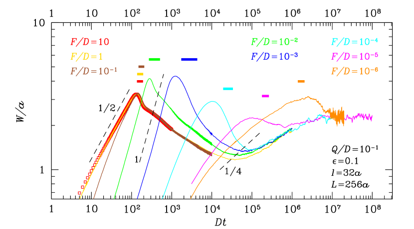
Figure S2: Roughness evolution for initial gap width $l=32$. Dashed lines have the indicated slopes and the horizontal solid bars indicate the range of collision times (average plus and minus one standard deviation).

The smaller values of the roughness before and after the formation of the GB in Fig. S2, compared with Fig. 4a of the main text, are consequences of the decrease of the gap width $l$.

The change in the edge length $L$ neither affects the initial roughening nor the relaxation after the GB formation because there are not effects of the finite lateral size in those regimes. As explained in Sec. SI.III, this length affects only the stationary roughness, which increases as $L^{1/2}$.

S.V Collision time in the high coverage regime

Fig. S3 shows the collision times scaled by the attachment rate $Q$ and by the dimensionless gap width $l/a$, as a function of $\epsilon F/D$. The data were obtained for different values of the detachment rate $0.01\leq\epsilon\leq 0.1$ and in different edge lengths $L$. This scaled plot shows that

$$t_{c}\sim 0.5\frac{l/a}{Q},$$ (S44)

independently of the other model parameters.

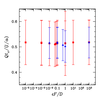
Figure S3: Scaled collision time as a function of the flux-diffusion ratio $F/D$. Different colors distinguish the different gap widths $l$.

S.VI Roughness evolution for $Q/D={10}^{-3}$

Fig. S2 shows the roughness evolution for $Q/D={10}^{-3}$ and several flux rates $F$, with the other parameters equal to those of Fig. 2a of the main text.

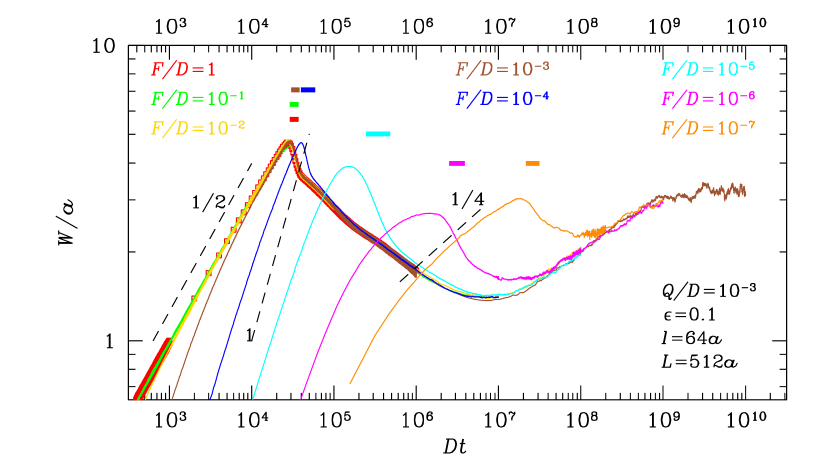
Figure S4: Roughness evolution for several values of the flux. Dashed lines have the indicated slopes and horizontal solid bars indicate the collision times (average plus and minus one standard deviation).

This is a case of large diffusion coefficient of particles in the gap in comparison with the attachment rate. It suppresses the unstable regime (diffusion-limited), as revealed by the absence of a slope larger than $1$ in those plots.

S.VII Roughness evolution for small detachment rate ($\epsilon=0.01$)

Fig. S5 shows the roughness evolution for three flux rates $F$, with the same parameters of Fig. 2a of the main text except $\epsilon=0.01$.

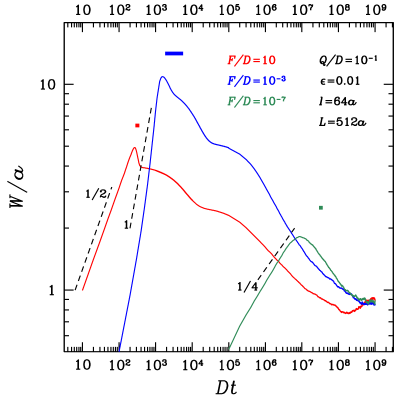
Figure S5: Roughness evolution with small detachment rate, for several values of the flux. Dashed lines have the indicated slopes.

References

- [1] Jichen Dong, Leining Zhang, and Feng Ding. Kinetics of graphene and 2D materials growth. Adv. Mater., 31:1801583, 2019.
- [2] Pinshane Y. Huang, Carlos S. Ruiz-Vargas, Arend M. Van Der Zande, William S. Whitney, Mark P. Levendorf, Joshua W. Kevek, Shivank Garg, Jonathan S. Alden, Caleb J. Hustedt, Ye Zhu, Jiwoong Park, Paul L. McEuen, and David A. Muller. Grains and grain boundaries in single-layer graphene atomic patchwork quilts. Nature, 469(7330):389–392, 2011.
- [3] Xiaozhi Xu, Zhihong Zhang, Lu Qiu, Jianing Zhuang, Liang Zhang, Huan Wang, Chongnan Liao, Huading Song, Ruixi Qiao, Peng Gao, Zonghai Hu, Lei Liao, Zhimin Liao, Dapeng Yu, Enge Wang, Feng Ding, Hailin Peng, and Kaihui Liu. Ultrafast growth of single-crystal graphene assisted by a continuous oxygen supply. Nature Nanotech., 11:930–935, 2016.
- [4] Alexandre Budiman Taslim, Hideaki Nakajima, Yung-Chang Lin, Yuki Uchida, Kenji Kawahara, Toshiya Okazaki, Kazu Suenaga, Hiroki Hibino, and Hiroki Ago. Synthesis of sub-millimeter single-crystal grains of aligned hexagonal boron nitride on an epitaxial Ni film. Nanoscale, 11:14668, 2019.
- [5] Hao Ying, Arden Moore, Jie Cui, Yaoyao Liu, Deshuai Li, Shuo Han, Yuan Yao, Zhiwei Wang, Lei Wang, and Shanshan Chen. Tailoring the thermal transport properties of monolayer hexagonal boron nitride by grain size engineering. 2D Materials, 7:015031, 2020.
- [6] Jun Lin, Scott Monaghan, Neha Sakhuja, Farzan Gity, Ravindra Kumar Jha, Emma M Coleman, James Connolly, Conor P Cullen, Lee A Walsh, Teresa Mannarino, Michael Schmidt, Brendan Sheehan, Georg S Duesberg, Niall McEvoy, Navakanta Bhat, Paul K Hurley, Ian M Povey, and Shubhadeep Bhattacharjee. Large-area growth of Mo at temperatures compatible with integrating back-end-of-line functionality. 2D Materials, 8:025008, 2021.
- [7] Lixuan Liu, Kun Ye, Changqing Lin, Zhiyan Jia, Tianyu Xue, Anmin Nie, Yingchun Cheng, Jianyong Xiang, Congpu Mu, Bochong Wang, Fusheng Wen, Kun Zhai, Zhisheng Zhao, Yongji Gong, Zhongyuan Liu, and Yongjun Tian. Grain-boundary-rich polycrystalline monolayer W film for attomolar-level sensors. Nature Commun., 12:3870, 2021.
- [8] Vinod K. Sangwan, Hong-Sub Lee, Hadallia Bergeron, Itamar Balla, Megan E. Beck, Kan-Sheng Chen, and Mark C. Hersam. Multi-terminal memtransistors from polycrystalline monolayer molybdenum disulfide. Nature, 554:500–504, 2018.
- [9] Yingqiu Zhou, Syed Ghazi Sarwat, Gang Seob Jung, Markus J. Buehler, Harish Bhaskaran, and Jamie H. Warner. Grain boundaries as electrical conduction channels in polycrystalline monolayer W. ACS Appl. Mater. Interfaces, 11:10189–10197, 2019.
- [10] Zhuhua Zhang, Yang Yang, Fangbo Xu, Luqing Wang, and Boris I. Yakobson. Unraveling the sinuous grain boundaries in graphene. Adv. Funct. Mater., 25:367–373, 2015.
- [11] Hui Zhang, Yue Yu, Xinyue Dai, Jinshan Yu, Hua Xu, Shanshan Wang, Feng Ding, and Jin Zhang. Probing atomic-scale fracture of grain boundaries in low-symmetry 2D materials. Small, 17:2102739, 2021.
- [12] Jaechul Ryu, Youngsoo Kim, Dongkwan Won, Nayoung Kim, Jin Sung Park, Eun-Kyu Lee, Donyub Cho, Sung-Pyo Cho, Sang Jin Kim, Gyeong Hee Ryu, Hae-A-Seul Shin, Zonghoon Lee, Byung Hee Hong, and Seungmin Cho. Fast synthesis of high-performance graphene films by hydrogen-free rapid thermal chemical vapor deposition. ACS Nano, 8:950–956, 2014.
- [13] Gwan-Hyoung Lee, Ryan C. Cooper, Sung Joo An, Sunwoo Lee, Arend van der Zande, Nicholas Petrone, Alexandra G. Hammerberg, Changgu Lee, Bryan Crawford, Warren Oliver, Jeffrey W. Kysar, and James Hone. High-strength chemical-vapor-deposited graphene and grain boundaries. Science, 340:1073–1076, 2013.
- [14] Vasilii I. Artyukhov, Yuanyue Liu, and Boris I. Yakobson. Equilibrium at the edge and atomistic mechanisms of graphene growth. Proc. Natl. Acad. Sci., 109:15136–15140, 2012.
- [15] Ksenia V. Bets, Vasilii I. Artyukhov, and Boris I. Yakobson. Kinetically determined shapes of grain boundaries in graphene. ACS Nano, 15:4893–4900, 2021.
- [16] Shuai Chen, Junfeng Gao, Bharathi M. Srinivasan, Gang Zhang, Ming Yang, Jianwei Chai, Shijie Wang, Dongzhi Chi, and Yong-Wei Zhang. Revealing the grain boundary formation mechanism and kinetics during polycrystalline growth. ACS Appl. Mater. Int., 11:46090–46100, 2019.
- [17] Kasra Momeni, Yanzhou Ji, Yuanxi Wang, Shiddartha Paul, Sara Neshani, Dundar E. Yilmaz, Yun Kyung Shin, Difan Zhang, Jin-Wu Jiang, Harold S. Park, Susan Sinnott, Adri van Duin, Vincent Crespi, and Long-Qing Chen. Multiscale computational understanding and growth of 2D materials: a review. npj Computational Materials, 6:22, 2020.
- [18] Danielle Reifsnyder Hickey, Nadire Nayir, Mikhail Chubarov, Tanushree H. Choudhury, Saiphaneendra Bachu, Leixin Miao, Yuanxi Wang, Chenhao Qian, Vincent H. Crespi, Joan M. Redwing, Adri C. T. van Duin, and Nasim Alem. Illuminating invisible grain boundaries in coalesced single-orientation W monolayer films. Nano Lett., 21:6487–6495, 2021.
- [19] Shu Nie, Joseph M. Wofford, Norman C. Bartelt, Oscar D. Dubon, and Kevin F. McCarty. Origin of the mosaicity in graphene grown on Cu(111). Phys. Rev. B, 84:155425, 2011.
- [20] Esteban Meca, John Lowengrub, Hokwon Kim, Cecilia Mattevi, and Vivek B. Shenoy. Epitaxial graphene growth and shape dynamics on copper: Phase-field modeling and experiments. Nano Lett., 13:5692–5697, 2013.
- [21] Ping Wu, Yue Zhang, Ping Cui, Zhenyu Li, Jinlong Yang, and Zhenyu Zhang. Carbon dimers as the dominant feeding species in epitaxial growth and morphological phase transition of graphene on different Cu substrates. Phys. Rev. Lett., 114:216102, 2015.
- [22] Jianing Zhuang, Ruiqi Zhao, Jichen Dong, Tianying Yand, and Feng Ding. Evolution of domains and grain boundaries in graphene: A kinetic Monte Carlo simulation. Phys. Chem. Chem. Phys., 18:2932–2939, 2016.
- [23] Ruoyu Yue, Yifan Nie, Lee A Walsh, Rafik Addou, Chaoping Liang, Ning Lu, Adam T Barton, Hui Zhu, Zifan Che, Diego Barrera, Lanxia Cheng, Pil-Ryung Cha, Yves J Chabal, Julia W P Hsu, Jiyoung Kim, Moon J Kim, Luigi Colombo, Robert M Wallace, Kyeongjae Cho, and Christopher L Hinkle. Nucleation and growth of : Enabling large grain transition metal dichalcogenides. 2d Mater., 4:045019, 2017.
- [24] T. Michely and J. Krug. Islands, Mounds, and Atoms. Springer, 2003.
- [25] A. Pimpinelli and J. Villain. Physics of Crystal Growth. Cambridge University Press, 1998.
- [26] Yukio Saito. Statistical Physics of Crystal Growth. World Scientific, Singapore, 1996.
- [27] J. W. Evans, P. A. Thiel, and M. C. Bartelt. Morphological evolution during epitaxial thin film growth: Formation of 2D islands and 3D mounds. Surface Science Reports, 61(1):1 – 128, 2006.
- [28] Chaouqi Misbah, Olivier Pierre-Louis, and Yukio Saito. Crystal surfaces in and out of equilibrium: A modern view. Rev. Mod. Phys., 82:981–1040, Mar 2010.
- [29] M. Einax, W. Dieterich, and P. Maass. Colloquium: Cluster growth on surfaces: Densities, size distributions, and morphologies. Rev. Mod. Phys., 85:921–939, Jul 2013.
- [30] P. Gaillard, T. Chanier, L. Henrard, P. Moskovkin, and S. Lucas. Multiscale simulations of the early stages of the growth of graphene on copper. Surf. Sci., 637-638:11–18, 2015.
- [31] Gwilym Enstone, Peter Brommer, David Quigley, and Gavin R. Bell. Enhancement of island size by dynamic substrate disorder in simulations of graphene growth. Phys. Chem. Chem. Phys., 18:15102–15109, 2016.
- [32] T. J. Oliveira and F. D. A. Aarão Reis. Scaling in reversible submonolayer deposition. Phys. Rev. B, 87:235430, Jun 2013.
- [33] Luca Gagliardi and Olivier Pierre-Louis. Controlling anisotropy in 2d microscopic models of growth. Journal of Computational Physics, 452:110936, 2022.
- [34] Yukio Saito, Matthieu Dufay, and Olivier Pierre-Louis. Nonequilibrium cluster diffusion during growth and evaporation in two dimensions. Phys. Rev. Lett., 108:245504, Jun 2012.
- [35] F. D. A. Aarão Reis and O. Pierre-Louis. Interface collisions. Phys. Rev. E, 97:040801(R), 2018.
- [36] A.-L. Barabási and H. E. Stanley. Fractal Concepts in Surface Growth. Cambridge University Press, New York, USA, 1995.
- [37] J. Krug. Origins of scale invariance in growth processes. Advances in Physics, 46(2):139–282, 1997.
- [38] S. F. Edwards and D. R. Wilkinson. The surface statistics of a granular aggregate. Proc. R. Soc. Lond. A, 381:17–31, 1982.
- [39] T. A. de Assis and F. D. A. A. Reis. Relaxation after a change in the interface growth dynamics. Phys. Rev. E, 89:062405, 2014.
- [40] T. A. de Assis and F. D. A. A. Reis. Smoothening in thin-film deposition on rough substrates. Phys. Rev. E, 92:052405, 2015.
- [41] O. Pierre-Louis and C. Misbah. Dynamics and fluctuations during MBE on vicinal surfaces. I. Formalism and results of linear theory. Phys. Rev. B, 58:2259–2275, Jul 1998.
- [42] Wenqian Yao, Bin Wu, and Yunqi Liu. Growth and grain boundaries in 2D materials. ACS Nano, 14:9320–9346, 2020.
- [43] Hui Cai, Yiling Yu, Alexander A. Puretzky Yu-Chuan Lin, David B. Geohegan, and Kai Xiao. Heterogeneities at multiple length scales in 2D layered materials: From localized defects and dopants to mesoscopic heterostructures. Nano Res., 14:1625–1649, 2021.
- [44] Jichen Dong, Leining Zhang, Bin Wu, Feng Ding, and Yunqi Liu. Theoretical study of chemical vapor deposition synthesis of graphene and beyond: Challenges and perspectives. J. Phys. Chem. Lett., 12:7942–7963, 2021.
- [45] Ziyi Han, Lin Li, Fei Jiao, Gui Yu, Wenping Hua, Zhongming Wei, and Dechao Geng. Continuous orientated growth of scaled single-crystal 2D monolayer films. Nanoscale Adv., 3:6545–6567, 2021.
- [46] Zheng Wei, Qinqin Wang, Lu Li, Rong Yang, and Guangyu Zhang. Monolayer Mo epitaxy. Nano Res., 14:1598–1608, 2021.
- [47] Emil Annevelink, Zhu-Jun Wang, Guocai Dong, Harley T. Johnson, and Pascal Pochet. A moiré theory for probing grain boundary structure in graphene. Acta Mater., 217:117156, 2021.
- [48] Kirill A. Bokai, Viktor O. Shevelev, Dmitry Marchenko, Anna A. Makarova, Vladimir Yu. Mikhailovskii, Alexei A. Zakharov, Oleg Yu. Vilkov, Maxim Krivenkov, Denis V. Vyalikh, and Dmitry Yu. Usachov. Visualization of graphene grain boundaries through oxygen intercalation. Appl. Surf. Sci., 565:150476, 2021.
- [49] S. Clarke and D. D. Vvedensky. Growth kinetics and step density in reflection high-energy electron diffraction during molecular-beam epitaxy. J. Appl. Phys., 63:2272, 1988.
- [50] R. Ghez and S. S. Iyer. The kinetics of fast steps on crystal surfaces and its application to the molecular beam epitaxy of silicon. IBM Journal of Research and Development, 32(6):804–818, 1988.
- [51] Russel E. Caflisch, Weinan E, Mark F. Gyure, Barry Merriman, and Christian Ratsch. Kinetic model for a step edge in epitaxial growth. Phys. Rev. E, 59:6879–6887, Jun 1999.