Core structure of static ferrodark solitons in a spin-1 Bose-Einstein condensate

Abstract

We develop an analytical description of static ferrodark solitons, the $\mathbb{Z}_{2}$ topological defects in the magnetic order, in the easy-plane phase of ferromagnetic spin-1 Bose-Einstein condensates. We find that the type-I ferrodark soliton has a single width while the type-II ferrodark soliton exhibits two characteristic length scales. The proposed ansatzes show excellent agreement with numerical results. Spin-singlet amplitudes, nematic tensor densities and nematic currents of ferrodark solitons are also discussed. The $\mathbb{Z}_{2}$ topological defects in the mass superfluid order, dark-dark-dark vector solitons, are obtained exactly in the parameter regime where exact ferrodark solitons exist. The dark-dark-dark vector soliton has higher excitation energy than ferrodark solitons.

I Introduction

A spin-1 Bose-Einstein condensate (BEC) is a coherent state constituted by atoms occupying hyperfine spin levels $\ket{F=1,m=+1,0,-1}$ that interact via spin-mixing collisions, exhibiting superfluidity and magnetic orders Ho (1998); Ohmi and Machida (1998); Stenger et al. (1998); Sadler et al. (2006); Stamper-Kurn and Ueda (2013); Kawaguchi and Ueda (2012). This spinor superfluid supports topological excitations that are absent in scalar and two-component BECs, adding novel features to phenomena such as the Berezinskii-Kosterlitz-Thouless transitions James and Lamacraft (2011); Kobayashi (2019) and out-of-equilibrium processes in superfluids, including Kibble-Zurek mechanism Saito et al. (2007a); Damski and Zurek (2007), phase ordering Lamacraft (2007); Mukerjee et al. (2007); Williamson and Blakie (2016a, 2017); Symes and Blakie (2017); Schmied et al. (2019a); Bourges and Blakie (2017) and thermalization processes Barnett et al. (2011); Fujimoto et al. (2019). It also provides, additional to magnetic thin films, a prominent platform for exploring quantum magnetism.

In the presence of a magnetic field along the $z$-axis, the ground state of a ferromagnetic spin-1 BEC can be in the easy-axis or broken-axisymmetry ferromagnetic phases, or the non-magnetized polar phase, each separated by a quantum phase transition Stamper-Kurn and Ueda (2013); Kawaguchi and Ueda (2012). The easy-plane phase, being the broken-axisymmetry phase with the magnetization lying in the $xy$-plane, is particularly interesting as it describes $XY$ magnetism and supports various unique topological excitations Williamson and Blakie (2016b); Turner (2009); Yu and Blakie (2021, 2022). A substantial amount of work has been devoted to studying quenches from the polar phase to the easy-plane phase by a change in the magnetic field Sadler et al. (2006); Saito et al. (2007b); Lamacraft (2007); Saito and Ueda (2005); Damski and Zurek (2007); Williamson and Blakie (2016a); Prüfer et al. (2018); Schmied et al. (2019b). Here polar core vortices are the relevant topological defects in two dimensions (2D) and determine the Kibble-Zurek scaling and the universal dynamic scaling in phase ordering at late times Williamson and Blakie (2016a). Domain wall structures also appear in the early stage of quenches due to the linear instability, but these domain walls are transient and continually decay to polar core vortices Saito et al. (2007b). In one-dimension (1D), domain walls/solitons are relevant defects and contribute the Kibble-Zurek scalings Damski and Zurek (2007); Saito et al. (2007a) and may play an important role in determining the universal scaling behaviors at later times of the quench  Prüfer et al. (2018); Schmied et al. (2019b) (i.e., the so-called non-thermal fixed point). However, little is known on the properties of the relevant domain walls/solitons in ferromagnetic spin-1 condensates.

An important question is what topological excitations are supported in the easy-plane phase of ferromagnetic spin-1 BECs ? Here the term “topological" refers to the winding number (2D) or the topological charge (1D) of the order parameter being nonzero. In a scalar BEC, vortices (2D) and dark solitons (1D) are the relevant topological excitations. In ferromagnetic spin-1 BECs, the magnetization serves as the local order parameter and quantifies the magnetic order associated with the $\textrm{SO}(3)$ rotational symmetry breaking. In the easy-plane phase, the spin vortices (defects associated with the continuous $\textrm{SO}(2)$ symmetry) are polar core vortices and Mermin-Ho vortices Stamper-Kurn and Ueda (2013); Kawaguchi and Ueda (2012); Mizushima et al. (2002); Kudo and Kawaguchi (2015), while kinks in the transverse magnetization (defects associated with the discrete $\mathbb{Z}_{2}$ symmetry) have been uncovered only recently thanks to the discovery of ferrodark solitons (FDSs) (also referred to as magnetic domain walls) Yu and Blakie (2021, 2022). The FDSs are magnetic kinks that connect transverse magnetic domains with opposite magnetizations, signified by the magnetization $\mathbf{F}$ vanishing at the core and changing its sign across the core. The superfluid density $n$ has a dip but does vanish at the core. The FDSs have two types and exhibit several distinct features, including positive inertial mass, stability against snake deformations, and oscillations in a linear potential due to the transition between the two types at the maximum speed Yu and Blakie (2021, 2022). The static profiles of FDSs have been studied in detail when $q\rightarrow 0$ Yu and Blakie (2021), where $q$ is the quadratic Zeeman energy of the atom in the magnetic field. However, at finite $q$, except for exactly solvable cases Yu and Blakie (2021, 2022), the core structure of FDSs remain unexplored.

In this paper we study the core structure of static FDSs for finite quadratic Zeeman energies ($q>0$) in the whole easy-plane phase. Accurate ansatzes are proposed and show good agreement with numerical results. In particular, we obtain the characteristic length scales analytically via consistent asymptotic analysis, finding that type-I FDS has a single length scale while type-II FDS requires two length scales to describe the width near-the-core and the width away-from-the-core, respectively. Spin-singlet amplitudes, nematic tensor densities and nematic currents of FDSs exhibit rich structure and provide a complete description of static FDSs. The dark-dark-dark vector solitons, which are the $\mathbb{Z}_{2}$ topological defects in the mass superfluid order, are also discussed.

II Spin-1 BECs

The mean-field Hamiltonian density of a spin-1 condensate reads

$${\cal H}=\frac{\hbar^{2}\left|\nabla\psi\right|^{2}}{2M}+\frac{g_{n}}{2}|\psi^{{\dagger}}\psi|^{2}+\frac{g_{s}}{2}|\psi^{{\dagger}}\mathbf{S}\psi|^{2}+q\psi^{{\dagger}}S^{2}_{z}\psi,$$ (1)

where the three-component wavefunction $\psi=(\psi_{+1},\psi_{0},\psi_{-1})^{T}$ describes the coherent atomic field in the three atomic hyperfine states $\ket{F=1,m=+1,0,-1}$, $M$ is the atomic mass, $g_{n}>0$ is the density-dependent interaction strength, $g_{s}$ is the spin-dependent interaction strength, and $S_{j=x,y,z}$ are the spin-1 matrices [$\mathbf{S}=(S_{x},S_{y},S_{z})$] Stamper-Kurn and Ueda (2013); Kawaguchi and Ueda (2012). The spin-dependent interaction terms describe spin-mixing collisions: $\ket{00}\leftrightarrow\ket{+1}\ket{-1}$, originating from the spin-dependence of the s-wave collisions Stamper-Kurn and Ueda (2013). The magnetic field is along the $z$-axis and $q$ denotes the quadratic Zeeman energy.

At the mean-field level, the dynamics of the field $\psi$ is governed by the spin-1 Gross-Pitaevskii equations (GPEs) which are obtained via the canonical equation $\partial\psi_{m}/\partial t=\delta{\cal H}/\delta(i\hbar\psi^{*}_{m})$:

$$i\hbar\frac{\partial\psi_{\pm 1}}{\partial t} =\left[H_{0}+g_{s}\left(n_{0}+n_{\pm 1}-n_{\mp 1}\right)+q\right]\psi_{\pm 1}+g_{s}\psi^{2}_{0}\psi^{*}_{\mp 1},$$ (2)

$$i\hbar\frac{\partial\psi_{0}}{\partial t} =\left[H_{0}+g_{s}\left(n_{+1}+n_{-1}\right)\right]\psi_{0}+2g_{s}\psi^{*}_{0}\psi_{+1}\psi_{-1},$$ (3)

where $H_{0}=-\hbar^{2}\nabla^{2}/2M+g_{n}n$, $n=\sum n_{m}$ is the total number density and $n_{m}=|\psi_{m}|^{2}$ is the component density.

A distinguishing feature of spin-1 BECs is that the system supports magnetic orders, with the magnetization $\mathbf{F}\equiv\psi^{{\dagger}}\mathbf{S}\psi=(F_{x},F_{y},F_{z})$ serving as the local order parameter. Here

$$F_{x} = \psi^{{\dagger}}S_{x}\psi=\frac{1}{\sqrt{2}}\left[\psi^{*}_{0}(\psi_{+1}+\psi_{-1})+{\rm H.c.}\right],$$ (4)

$$F_{y} = \psi^{{\dagger}}S_{y}\psi=\frac{i}{\sqrt{2}}\left[\psi^{*}_{0}(\psi_{+1}-\psi_{-1})-{\rm H.c.}\right],$$ (5)

$$F_{z} = \psi^{{\dagger}}S_{z}\psi=|\psi_{+1}|^{2}-|\psi_{-1}|^{2}.$$ (6)

It is convenient to introduce the transverse magnetization as the complex density

$$F_{\perp}\equiv F_{x}+iF_{y}=\sqrt{2}\left(\psi_{0}\psi^{*}_{+1}+\psi^{*}_{0}\psi_{-1}\right).$$ (7)

For ferromagnetic coupling $g_{s}<0$ (⁸⁷Rb,⁷Li), $|\mathbf{F}|>0$ and for anti-ferromagnetic coupling $g_{s}>0$ (²³Na), $\mathbf{F}=0$. At $q=0$, the system processes $\textrm{SO}(3)$ rotational symmetry and the total magnetization $\mathbf{M}=\int d\mathbf{r}\,{\mathbf{F}}$ is conserved. In the presence of a magnetic field ($q\neq 0$), the remaining symmetry is $\textrm{SO}(2)$ rotational symmetry, and yields to the conservation of the total magnetization along the $z$-axis $M_{z}=\int d\mathbf{r}F_{z}$. In contrast to binary BECs, a spin-1 BEC is not an incoherent mixture of condensates, i.e., the system does not process $\textrm{U}(1)\times\textrm{U}(1)\times\textrm{U}(1)$ symmetry Stamper-Kurn and Ueda (2013).

III Easy-plane phase

For a uniform ferromagnetic system ($g_{s}<0$) with total density $n_{b}$, the energy density is

$${\cal H}=\frac{1}{2}g_{n}n^{2}_{b}+\frac{g_{s}}{2}|\mathbf{F}|^{2}+q(n_{b}-n_{0}).$$ (8)

The uniform ground state is found by minimizing the free energy density ${\cal F}\equiv{\cal H}-p\,F_{z}$ Stenger et al. (1998); Zhang et al. (2003), where $p$ is the Lagrange multiplier. In the following we only consider $F_{z}=0$. Hence for $q>0$ the magnetization prefers to lie in the transverse plane, realizing an easy-plane ferromagnetic phase Stamper-Kurn and Ueda (2013); Kawaguchi and Ueda (2012). Plugging the wavefunction

$$\psi=\left(\sqrt{n_{+1}}e^{i\theta_{+1}},\sqrt{n_{0}}e^{i\theta_{0}},\sqrt{n_{-1}}e^{i\theta_{-1}}\right)^{T}$$ (9)

into the energy function Eq. (8), we obtain

$$E=2g_{s}n_{0}(n_{b}-n_{0})\cos^{2}\left[\theta_{0}-\frac{\theta_{+1}+\theta_{-1}}{2}\right]+\frac{g_{n}}{2}n_{b}^{2}+q(n_{b}-n_{0}).$$

The energy $E$ reaches the minimum when

$$2\theta_{0} = \theta_{+1}+\theta_{-1},$$ (11)

$$n_{0} = n^{g}_{0}=\frac{n_{b}(1+\tilde{q})}{2},$$ (12)

$$n_{\pm 1} = n^{g}_{\pm 1}=\frac{n_{b}(1-\tilde{q})}{4},$$ (13)

where $\tilde{q}\equiv-q/(2g_{s}n_{b})$. The ground-state magnetization reads

$$F_{\perp}^{g}(\tau)=n_{b}\sqrt{1-\tilde{q}^{2}}e^{i\tau},$$ (14)

where $\tau=\theta_{0}-\theta_{+1}=\theta_{-1}-\theta_{0}$ describes the orientation of the transverse magnetization [the $\textrm{SO}(2)$ rotational angle about the z axis ($e^{-i\tau S_{z}}$)], quantifying the magnetic order. The ground wavefunction can be written as

$$\psi^{g}(\theta,\tau)=\sqrt{n_{b}}e^{i\theta}e^{-i\tau S_{z}}\left(\sqrt{\frac{n^{g}_{+1}}{n_{b}}},\sqrt{\frac{n^{g}_{0}}{n_{b}}},\sqrt{\frac{n^{g}_{-1}}{n_{b}}}\right)^{T},$$ (15)

where $\theta$ describes the global U(1) phase and quantifies the mass superfluid order. Note that the choice of the global phase $\theta$ is not unique and depends on the realization of the spin rotation in spin states. For instance, for the state $e^{i\theta_{0}}\left(\sqrt{n^{g}_{+1}}e^{-i\tau},\sqrt{n^{g}_{0}},\sqrt{n^{g}_{-1}}e^{i\tau}\right)^{T}$, $\theta_{0}$ can be regarded as the global phase. Rearranging the phases in spin states, it becomes $e^{i\theta_{+1}}\left(\sqrt{n^{g}_{+1}},\sqrt{n^{g}_{0}}e^{i\tau},\sqrt{n^{g}_{-1}}e^{2\tau i}\right)^{T}$ and then $\theta=\theta_{+1}$.

The positiveness of component densities $n_{\pm 1}$ requires $q<-2g_{s}n_{b}$ which sets the parameter range of the easy-plane phase. Note that for $q<0$, under the constraint $M_{z}=0$, a fragmented state of mixed $F_{z}=n_{b}$ and $F_{z}=-n_{b}$ domains has lower energy than any uniform state Kawaguchi and Ueda (2012); Stamper-Kurn and Ueda (2013).

IV $\mathbb{Z}_{2}$ topological defects

In this section, we discuss $\mathbb{Z}_{2}$ topological defects in the easy-plane phase of a ferromagnetic BEC. Hereafter we consider 1D systems. It is useful to introduce the topological charge to characterize $\mathbb{Z}_{2}$ defects in the magnetic order

$$Q_{F_{\perp}}=\frac{1}{2|F^{g}_{\perp}|}\int^{\infty}_{-\infty}dx\,\partial_{x}F_{\perp}(x)$$ (16)

and the topological charge to characterize $\mathbb{Z}_{2}$ defects in the mass superfluid order

$$Q_{\psi}=\prod_{m=-1,0,1}Q_{\psi_{m}}$$ (17)

where

$$Q_{\psi_{m}}=\frac{1}{2|\psi^{g}_{m}|}\int^{\infty}_{-\infty}dx\,\partial_{x}\psi_{m}(x).$$ (18)

The topological charges can be also expressed in terms of relevant phases:

$$Q_{F_{\perp}}=\frac{1}{\pi}\int^{\infty}_{-\infty}dx\,\partial_{x}\tau(x),$$ (19)

and

$$Q_{\psi}=\frac{1}{\pi}\int^{\infty}_{-\infty}dx\,\partial_{x}\theta(x).$$ (20)

It should be understood that here the results are modulo 2. The $\textrm{SO}(2)$ spin rotation $e^{-i\pi S_{z}}$ and the $\textrm{U}(1)$ gauge transformation $e^{-i\pi}$ play the role of charge conjugation operators and change signs of $Q_{F_{\perp}}$ and $Q_{\psi}$, respectively. Note that the spin rotation $e^{-i\pi S_{z}}$ does not change sign of $Q_{\psi}$ and the gauge transformation $e^{-i\pi}$ keeps sign of $Q_{F_{\perp}}$ unchanged.

IV.1 $\mathbb{Z}_{2}$ defects in the magnetic order: ferrodark solitons

Let us consider two oppositely magnetized domains with $\tau=0$ and $\tau=\pi$ respectively and search for a magnetic kink $F_{\perp}(x)$ that interpolates the two domains, namely

$$F_{\perp}(-\infty)=F^{g}_{\perp}(\pi)\,\,\text{and}\,\,F_{\perp}(+\infty)=F^{g}_{\perp}(0)=-F_{\perp}(-\infty).$$ (21)

It was found that an Ising-type magnetic kink satisfies the condition Eq. (21), signified by $F_{\perp}$ vanishing at the core and changing its sign across the core. This kink was referred to as FDS Yu and Blakie (2022). Exact FDS solutions of Eqs. (2) and  (3) were found at $g_{s}=-g_{n}/2$ Yu and Blakie (2021, 2022):

$$F^{\rm I,II}_{\perp}(x) = |F_{\perp}^{g}|\tanh\left(\frac{x}{2\ell^{\rm I,II}_{\rm ex}}\right),$$ (22)

$$n^{\rm I,II}(x) = n_{b}\left[1-\frac{(1\mp\tilde{q})}{2}\operatorname{sech}^{2}\left(\frac{x}{2\ell^{\rm I,II}_{\rm ex}}\right)\right],$$ (23)

where $\ell^{\rm I,II}_{\rm ex}=\hbar/\!\sqrt{2g_{n}n_{b}M(1\mp\tilde{q})}$, and the minus and plus signs in front of $q$ are referred to as type-I and type-II FDSs, respectively. Note that $\ell^{\rm II}_{\rm ex}\leq\ell^{\rm I}_{\rm ex}$ with the equality holding at $q=0$. The corresponding wavefunctions read

$$\psi^{\rm I}_{\pm 1}(x)=\sqrt{n^{g}_{\pm 1}}\tanh\left(\frac{x}{2\ell^{\rm I}_{\rm ex}}\right),\quad\psi^{\rm I}_{0}(x)=\sqrt{n^{g}_{0}};$$ (24)

and

$$\psi^{\rm II}_{\pm 1}(x)=\sqrt{n^{g}_{\pm 1}},\quad\psi^{\rm II}_{0}(x)=\sqrt{n^{g}_{0}}\tanh\left(\frac{x}{2\ell^{\rm II}_{\rm ex}}\right).$$ (25)

At the core ($x=0$), the magnetization vanishes [$F^{\rm I,II}_{\perp}(0)=0$] while the superfluid density $n$ is finite [$n^{\rm I,II}(0)\neq 0$]. FDSs are topological defects in the magnetic order but not in the superfluid order, namely $Q_{F_{\perp}}=\pm 1$ [$Q_{F_{\perp}}=-1$ for anti-FDSs $e^{-i\pi S_{z}}\psi^{\rm I,II}(x)$] while $Q_{\psi}=0$.

The wavefunctions of FDSs Eqs. (24) and  (25) can be written as follows:

$$\psi^{\rm I}(x)=\left[|\psi^{\rm I}_{+1}|e^{-i\tau(x)},\quad|\psi^{\rm I}_{0}|,\quad|\psi^{\rm I}_{-1}|e^{i\tau(x)}\right]^{T},$$ (26)

$$\psi^{\rm II}(x)=\left[|\psi^{\rm II}_{+1}|,\quad|\psi^{\rm II}_{0}|e^{i\tau(x)},\quad|\psi^{\rm II}_{-1}|e^{i2\tau(x)}\right]^{T},$$ (27)

where $\tau(x)$ is a step function: $\tau(x<0)=-\pi$ and $\tau(x\geq 0)=0$. Hence type-I and type-II FDSs might be viewed as 1D analogies of polar core vortices and Mermin-Ho vortices, respectively.

We consider stationary excitations which satisfy $\psi_{+1}=\psi_{-1}$ [upon a $\textrm{SO}(2)$ spin rotation] and the stationary GPEs become

$$0 =\left[-\frac{\hbar^{2}}{2M}\frac{d^{2}}{dx^{2}}-\mu+2g_{n}n_{\pm 1}+(g_{n}+2g_{s})n_{0}+q\right]\psi_{\pm 1},$$ (28)

$$0 =\left[-\frac{\hbar^{2}}{2M}\frac{d^{2}}{dx^{2}}-\mu+g_{n}n_{0}+2(g_{n}+2g_{s})n_{\pm 1}\right]\psi_{0\phantom{+}},$$ (29)

where the chemical potential $\mu=(g_{n}+g_{s})n_{b}+q/2$ and the wavefunctions $\psi_{m}$ are chosen to be real. Clearly U(1) gauge transformations and $\textrm{SO}(2)$ spin rotations keep Eqs. (28) and (29) unchanged. At $g_{s}=-g_{n}/2$, Eqs. (28) and (29) become decoupled and admit exact type-I [Eq. (24)] and type-II [Eq. (25)] solutions. It is worth mentioning that the exactly solvable point is within the scope of a ⁷Li spin-1 BEC which has been prepared in a regime with a strong spin-dependent interaction Huh et al. (2020).

IV.2 $\mathbb{Z}_{2}$ defects in the mass superfluid order: dark-dark-dark vector solitons

There is another soliton solution $\psi(x)$ to the Eqs. (28) and (29) that satisfies

$$\psi(-\infty)=\psi^{g}(\pi,\tau)\,\,\text{and}\,\,\psi(+\infty)=\psi^{g}(0,\tau)=-\psi(-\infty),$$ (30)

and at $g_{s}=-g_{n}/2$:

$$\psi^{d}_{\pm 1}(x)=\sqrt{n^{g}_{\pm 1}}\tanh\left(\frac{x}{2\ell^{\rm I}_{\rm ex}}\right),\quad\psi^{d}_{0}(x)=\sqrt{n^{g}_{0}}\tanh\left(\frac{x}{2\ell^{\rm II}_{\rm ex}}\right).$$

(31)

Here we have chosen that $\tau=0$. The corresponding transverse magnetization and the total density read

$$F^{d}_{\perp}(x) = |F_{\perp}^{g}|\tanh\left(\frac{x}{2\ell^{\rm II}_{\rm ex}}\right)\tanh\left(\frac{x}{2\ell^{\rm I}_{\rm ex}}\right),$$ (32)

$$n^{d}(x) = n^{b}\left[1-\frac{1-\tilde{q}}{2}\operatorname{sech}\left(\frac{x}{2\ell^{\rm I}_{\rm ex}}\right)^{2}-\frac{1+\tilde{q}}{2}\operatorname{sech}\left(\frac{x}{2\ell^{\rm II}_{\rm ex}}\right)^{2}\right].$$

In the literature this soliton has been referred to as the dark-dark-dark (DDD) vector soliton Katsimiga et al. (2021). The DDD vector soliton is the $\mathbb{Z}_{2}$ topological defect in the mass superfluid order, characterized by changing sign of $\psi^{d}(x)$ across the core [accompanied by $n^{d}(0)=0$] and $Q_{\psi}=1$ [$Q_{\psi}=-1$ for the anti-DDD $e^{-i\pi}\psi^{d}(x)$]. The DDD vector soliton is not a topological defect in the magnetic order as the transverse magnetization $F^{d}_{\perp}$ does not change sign across the core [although $F^{d}_{\perp}(0)=0$] and $Q_{F_{\perp}}=0$. Note that the spin rotation $e^{-i\pi S_{z}}$ does not change the sign of $Q_{\psi}$, i.e., $Q_{\psi}=1$ for $e^{-i\pi S_{z}}\psi^{d}(x)$ and $Q_{\psi}=-1$ for $e^{-i\pi S_{z}}e^{-i\pi}\psi^{d}(x)$. Typical profiles of FDSs and the DDD vector soliton are shown in Fig. 1.

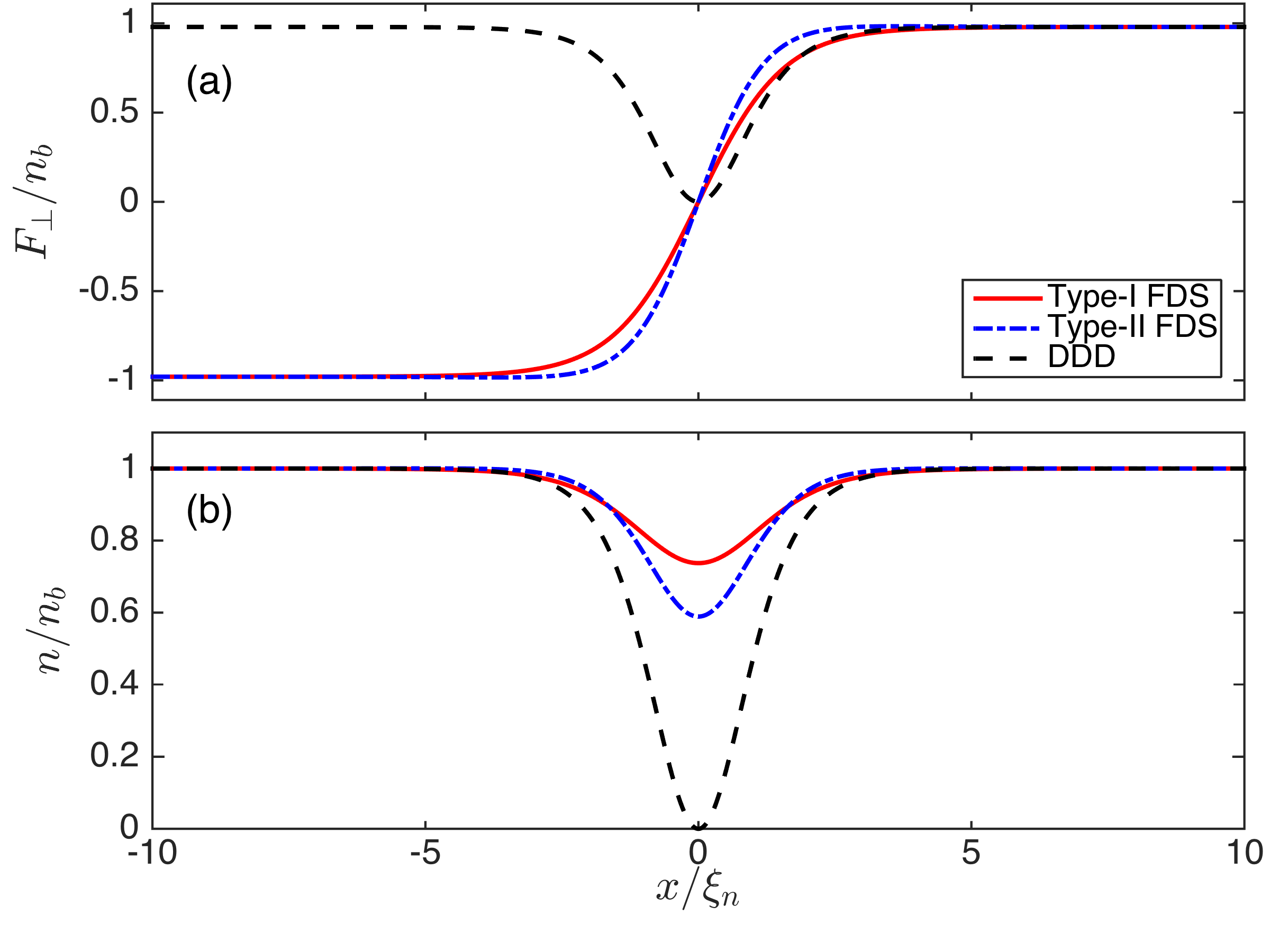
Figure 1: The transverse magnetization (a) and the density (b) of FDSs and the DDD at $g_{s}=-0.3g_{n}$ and $\tilde{q}=0.2$. Here $\xi_{n}=\hbar/\sqrt{n_{b}g_{n}M}$.

The energy of a DDD vector soliton is higher than a FDS in the parameter region where the DDD vector soliton is supported foo (a) (see Fig. 2). Here the numerical solutions are obtained using a gradient flow method Lim and Bao (2008); Bao and Lim (2008). We quantify the soliton energy as the excess grand canonical energy over that of the ground state, i.e. as $\delta K\equiv K[\psi]-K_{g}$, where

$$K[\psi]=\int dx\,\left({\cal H}[\psi]-\mu n_{b}\right),$$ (34)

and

$$K_{g}=\int dx\,\left({\cal H}[\psi^{g}]-\mu n_{b}\right)=\frac{n^{2}_{b}[g_{s}(\tilde{q}^{2}-1)-g_{n}]}{2}L.$$ (35)

Here $L$ is the system size.

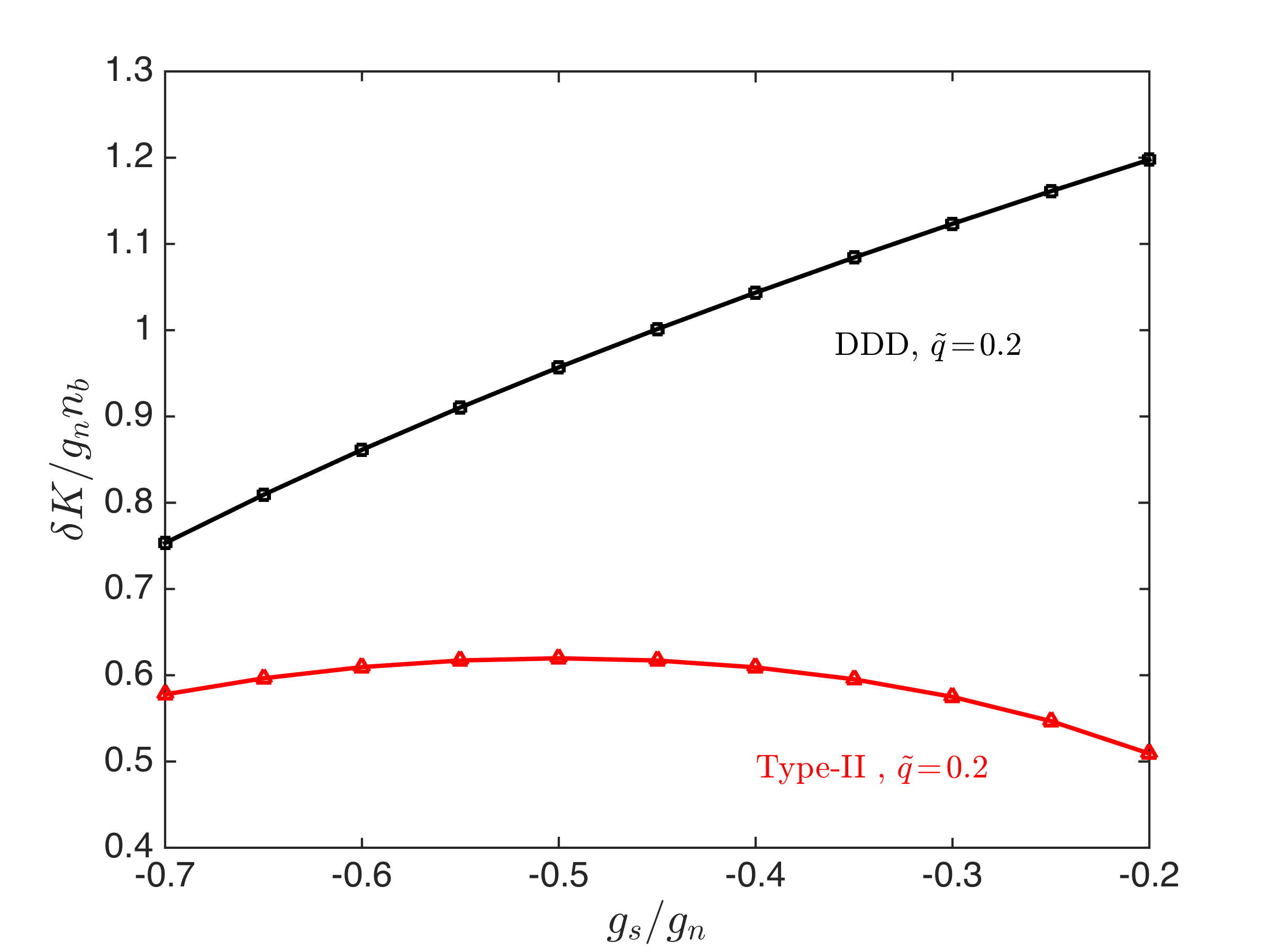
Figure 2: Numerical results for the energies of type-II FDSs (red triangles) and DDD solitons (black squares) at $\tilde{q}=0.2$. Here only the type-II FDS energy curve is presented as the type-I FDS always has lower energy (see Sec. V.3).

In the following, we focus on analyzing the core structure of FDSs away from the exactly solvable regime.

V Core structure for a finite quadratic Zeeman shift

The fundamental properties of FDSs do not qualitatively change away from the exactly solvable regime ($g_{s}/g_{n}=-1/2$, $0<q<-2g_{s}n_{b}$). However, the characteristic length scales do vary as $g_{s}$ changes and have been characterized in the $q\rightarrow 0$ limit in Ref. Yu and Blakie (2021). This limit allows us to connect, through $\textrm{SO}(3)$ spin rotations, various different degenerate forms of the FDS. At $q=0$, the core structure was conveniently analyzed using a particular rotated state referred to as the sine-Gordon representation. For $q>0$, the $\textrm{SO}(3)$ symmetry is broken by the magnetic field and the sine-Gordon like solitons are no longer stationary solutions Yu and Blakie (2021). A different scheme is therefore required to obtain the widths of FDSs.

V.1 Type-I FDSs

Away from the exactly solvable regime, we propose the following ansatz for type-I FDSs

$$\psi^{\rm I}_{\pm 1}(x) =\sqrt{n^{g}_{\pm 1}}\tanh\left(\frac{x}{2\ell^{\rm I}}\right),$$ (36)

$$\psi^{\rm I}_{0}(x) =\frac{c^{\rm I}}{g^{\rm I}+\cosh\left(\frac{x}{\ell^{\rm I}}\right)}+\sqrt{n^{g}_{0}},$$ (37)

where $\ell^{\rm I}$ is a length scale describing the core size and $g^{\rm I}$ is introduced to adjust the core structure. For $x\gg\ell^{\rm I}$, $\psi_{\pm 1}(x)\sim\sqrt{n^{g}_{\pm 1}}(1-2e^{-x/\ell^{\rm I}})$ and $\psi^{\rm I}_{0}(x)\sim 2c^{\rm I}e^{-x/\ell^{\rm I}}+\sqrt{n^{g}_{0}}$. This ansatz solves Eqs. (28) and (29) asymptotically ($x\gg\ell^{\rm I}$) if $\ell^{\rm I}$ is a physically acceptable (real and positive) root of the polynomial equation

$$4M^{2}(g_{n}+g_{s})(4g^{2}_{s}n_{b}-q^{2})y^{4}+4g_{n}g_{s}Mn_{b}\hbar^{2}y^{2}-g_{s}\hbar^{4}=0$$

(38)

and

$$c^{\rm I}=-\frac{(g_{n}+2g_{s})(2g_{s}n_{b}+q)\sqrt{2n_{b}-\frac{q}{g_{s}}}}{4\sqrt{g_{s}\left[g_{s}n_{b}^{2}(g_{n}+2g_{s})^{2}-q^{2}(g_{n}+g_{s})\right]}+2g_{n}q}.$$ (39)

Two positive roots of Eq. (38) are

$$y_{\pm}=\sqrt{\frac{g_{s}\hbar^{2}}{2M\left(g_{n}g_{s}n_{b}\pm\sqrt{g_{s}[g_{s}n_{b}^{2}(g_{n}+2g_{s})^{2}-q^{2}(g_{n}+g_{s})]}\right)}}.$$

It is easy to check that $y_{+}|_{g_{s}=-g_{n}/2}=\ell^{\rm I}_{\rm ex}$ [where $\ell^{\rm I}_{\rm ex}$ was introduced after Eq. (23)], hence we identify

$$\ell^{\rm I}=y_{+}.$$ (41)

As $g_{s}\rightarrow-g_{n}/2$, $c^{\rm I}\rightarrow 0$. Moreover $c^{\rm I}$ changes the sign when $g_{s}$ crosses the exactly solvable point $-g_{n}/2$ [Fig. 3(b)], inducing a hump or dip in $\psi_{0}$ [Fig. 4 (d) and (d^′)].

Near the core $x\sim 0$, solving Eqs. (28) and  (29) to leading order, we obtain

$$g_{n}\left(\frac{c^{\rm I}}{g^{\rm I}+1}+d\right)^{3}-\mu\left(\frac{c^{\rm I}}{g^{\rm I}+1}+d\right)+\frac{2c^{\rm I}\hbar^{2}}{4(g^{\rm I}+1)^{2}(\ell^{\rm I})^{2}M}=0,$$

(42)

which determines the value of $g^{\rm I}$. Neglecting the last term of Eq. (42), we obtain

$$g^{\rm I}=\frac{c^{\rm I}}{\sqrt{\mu/g_{n}}-\sqrt{n^{g}_{0}}}-1.$$ (43)

Evaluating the last term in Eq. (42) using the result in Eq. (43) verifies that it is small, justifying the approximation used here.

The results in Fig. 4 compare the ansatz in Eqs. (36) and (37) against numerical solution of the GPEs. This comparison shows that the ansatz we have developed provides a very good description of the core structure of the soliton over a wide range of parameters.

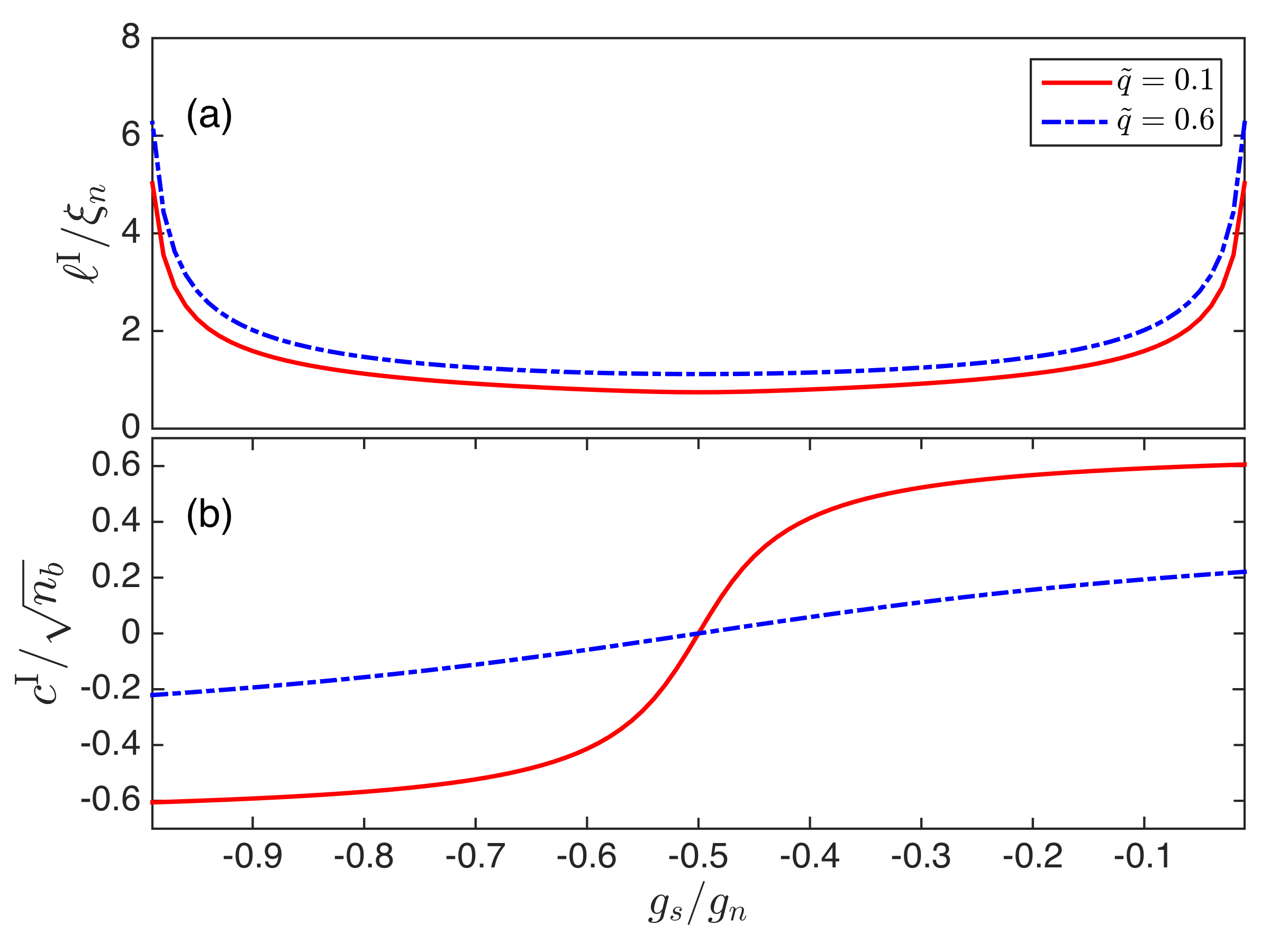
Figure 3: Key parameters in the ansatz of type-I FDSs given in Eqs. (36) and (37) as functions of $g_{s}$ for $\tilde{q}=0.1$ and $\tilde{q}=0.6$.

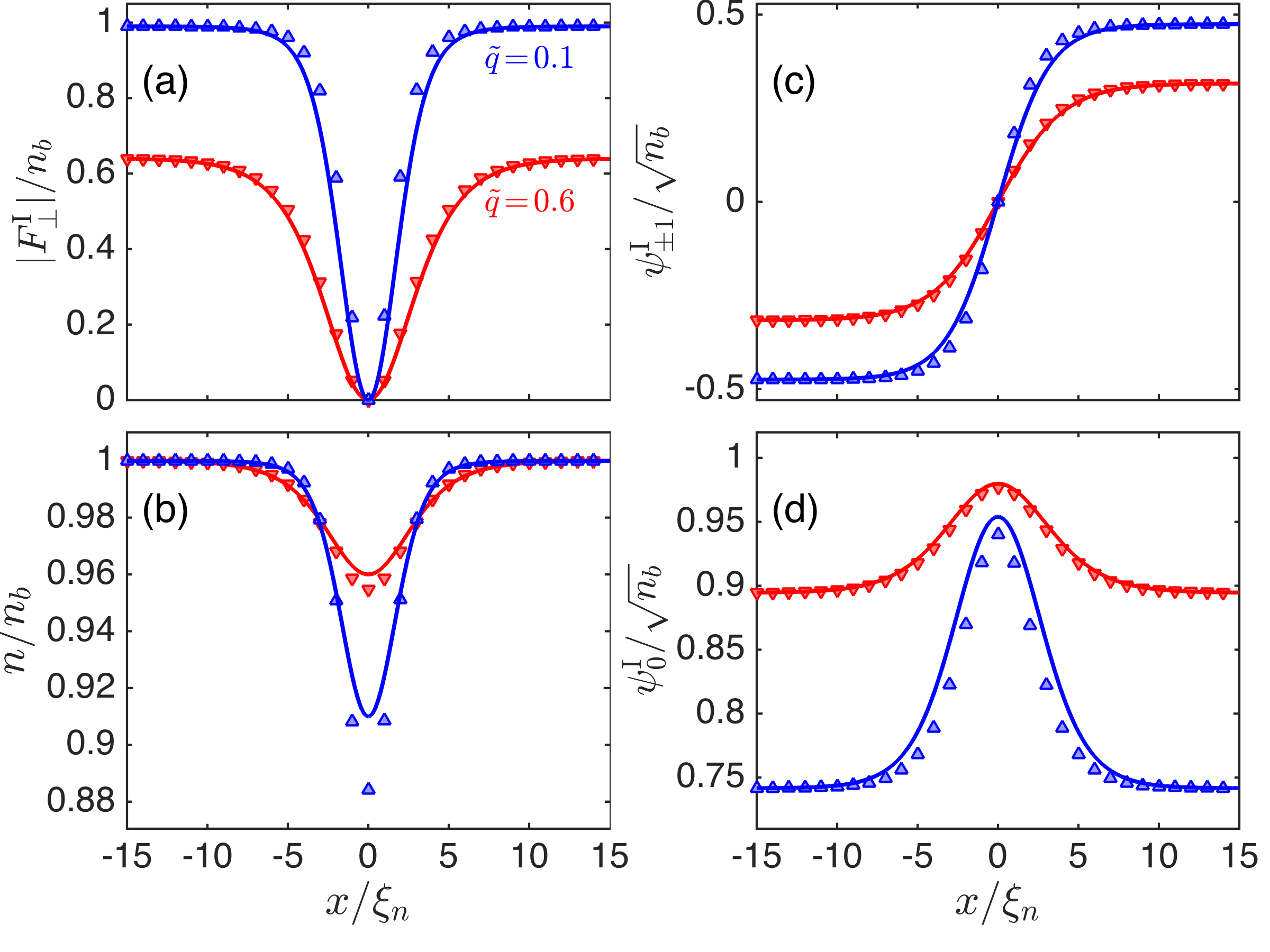
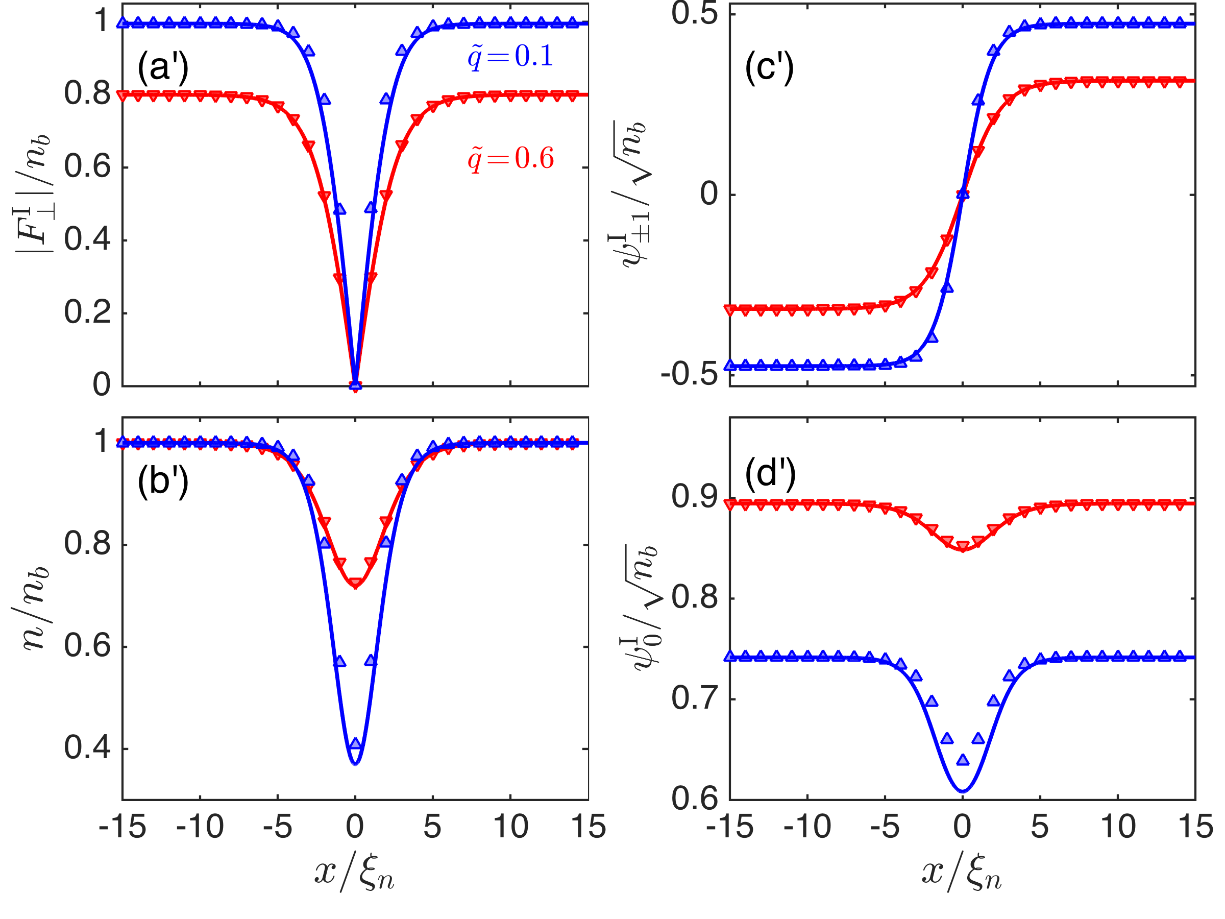
Figure 4: A comparison between analytical predictions of type-I FDSs (solid lines) and numerical results (markers) at $\tilde{q}=0.1$ and $\tilde{q}=0.6$. (a), (b), (c) and (d) are for $g_{s}/g_{n}=-0.1$ ; (a^′), (b^′), (c^′) and (d^′) are for $g_{s}/g_{n}=-0.7$.

V.2 Type-II FDSs

At the exactly solvable point Eqs. (28) and (29) admit another exact solution – the type-II soliton given in Eq. (25). Away from the exactly solvable point, the core structure of type-II FDSs exhibits additional complexity which requires two length scales to describe the core widths near and away from the center. We hence propose the following ansatz

$$\psi^{\rm II}_{0}(x) =\sqrt{n^{g}_{0}}\tanh\left(\frac{x}{2\ell^{\rm II}_{a}}\right)\left(\frac{c^{\rm II}/\kappa}{\cosh\left(\frac{x}{\ell^{\rm II}_{b}}\right)}+1\right),$$ (44)

$$\psi^{\rm II}_{\pm 1}(x) =\frac{c^{\rm II}}{\cosh\left(\frac{x}{\ell^{\rm II}_{b}}\right)}+\sqrt{n^{g}_{\pm 1}},$$ (45)

where we assume $\ell^{\rm II}_{b}>\ell^{\rm II}_{a}$. For $x\gg\ell^{\rm I}_{b}$, $\psi^{\rm II}_{0}(x)\sim\sqrt{n^{g}_{0}}\left[1+2(c^{\rm II}/\kappa)e^{-x/\ell^{\rm II}_{b}}\right]$ and $\psi^{\rm II}_{\pm 1}(x)\sim\sqrt{n^{g}_{\pm 1}}+2c^{\rm II}e^{-x/\ell^{\rm II}_{b}}$. Solving Eqs. (28) and  (29) asymptotically, we obtain that $\ell^{\rm II}_{b}$ has to be a root of Eq. (38) and

$$\kappa=\frac{g_{n}q-2g_{s}\sqrt{n_{b}^{2}(g_{n}+2g_{s})^{2}-\frac{q^{2}(g_{n}+g_{s})}{g_{s}}}}{2g_{s}(g_{n}+2g_{s})\sqrt{\frac{2q}{g_{s}}+4n_{b}}}.$$ (46)

If the core was characterized by a single length scale, the value of $\ell^{\rm II}_{b}$ could be easily set to be $y_{+}$, as it gives rise to the right value at the exactly solvable point, namely $y_{+}|_{g_{s}=-g_{n}/2}=\ell^{\rm II}_{\rm ex}$. However, when the other length scale $\ell^{\rm II}_{a}$ is introduced, a different scenario becomes possible to connect to the exactly solvable point, i.e., $c^{\rm II}\rightarrow 0$ and $\ell^{\rm II}_{a}\rightarrow\ell^{\rm II}_{\rm ex}$ as $g_{s}\rightarrow-g_{n}/2$. The appropriate choice for $\ell_{b}^{\rm II}$ to provide a consistent solution is

$$\ell^{\rm II}_{b}=y_{-}=\ell^{\rm I}.$$ (47)

Near the core $x\sim 0$, solving Eqs. (28) and  (29) to leading order, we obtain

$$\ell^{\rm II}_{a}=\sqrt{\frac{\hbar^{2}}{2M\left(2\mu-{\cal D}\right)}}$$ (48)

with

$${\cal D}=4(g_{n}+2g_{s})(c^{\rm II}+\sqrt{n_{\pm 1}})^{2}+\frac{3c^{\rm II}\hbar^{2}}{(\ell^{\rm I})^{2}M(c^{\rm II}+\kappa)},$$ (49)

where $c^{\rm II}$ is determined by the real solution of

$$2g_{n}\left(c^{\rm II}+\sqrt{n_{\pm 1}}\right)^{3}+\frac{c^{\rm II}\hbar^{2}}{2M(\ell^{\rm I})^{2}}+(q-\mu)\left(c^{\rm II}+\sqrt{n_{\pm 1}}\right)=0.$$

It is easy to check that as $g_{s}\rightarrow-g_{n}/2$, $c^{\rm II}\rightarrow 0$, ${\cal D}\rightarrow 0$ and $\ell^{\rm II}_{a}\rightarrow\ell^{\rm II}_{\rm ex}$. Consistently, the two scales we obtained indeed satisfy the working assumption $\ell^{\rm II}_{b}>\ell^{\rm II}_{a}$ [Fig. 5(a)]. The sign change of $c^{\rm II}$ across $g_{s}=-g_{n}/2$ (Fig. 5), yields a hump or a dip in $\psi_{\pm 1}$ (Fig. 6). Note that the other working assumption (i.e. $\ell^{\rm II}_{b}<\ell^{\rm II}_{a}$) does not lead to a consistent solution. A comparison of the two-scale ansatz Eqs. (44) and (45) to numerical solutions of the GPEs is presented in Fig. 6. These results validate that this ansatz effectively captures the core structure of type-II FDSs over a wide parameter regime. It is worthwhile to mention that at $q\neq 0$ stationary type-I and type-II FDSs are orthogonal, namely, the overlap $\int dx\,(\psi^{\rm I})^{{\dagger}}\psi^{\rm II}=0$. For propagating FDSs, the overlap between the two types does not vanish and reaches the maximum value at the speed limit Yu and Blakie (2022).

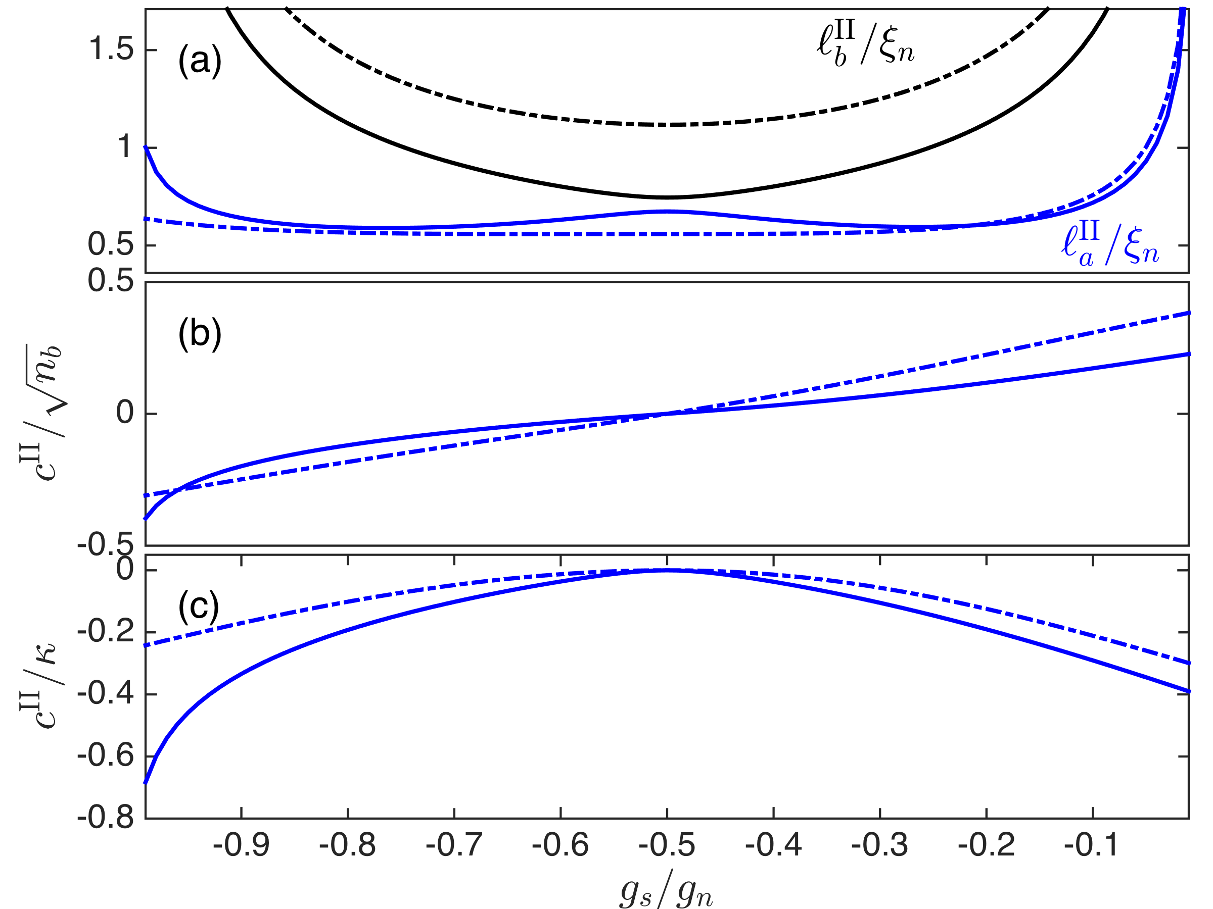
Figure 5: Key parameters in the ansatz of type-II FDSs [Eqs. (44) and (45)] as functions of $g_{s}$ for $\tilde{q}=0.1$ (solid lines) and $\tilde{q}=0.6$ (dash-dotted lines).

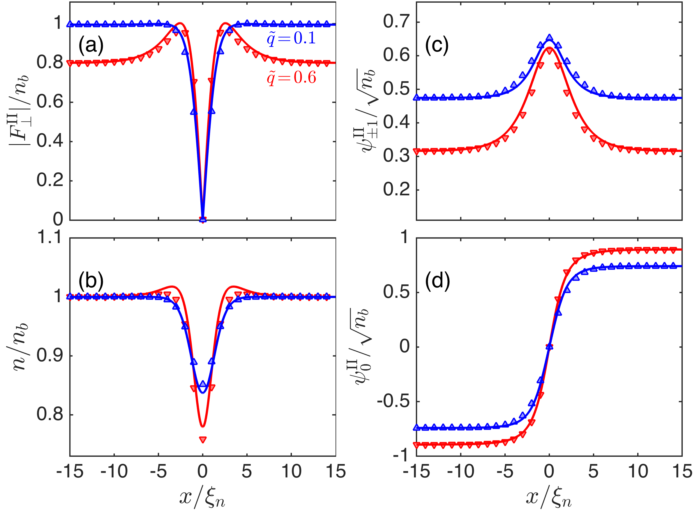
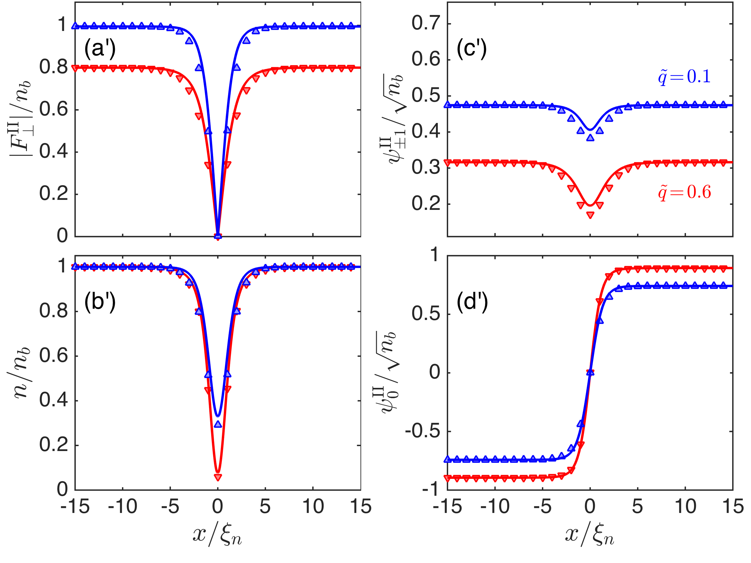
Figure 6: A comparison between analytical predictions of type-II FDSs (solid lines) and numerical results (markers) at $\tilde{q}=0.1$ and $\tilde{q}=0.6$. (a), (b),(c) and (d) are for $g_{s}/g_{n}=-0.1$ ; (a^′), (b^′), (c^′) and (d^′) are for $g_{s}/g_{n}=-0.7$.

V.3 Excitation energies

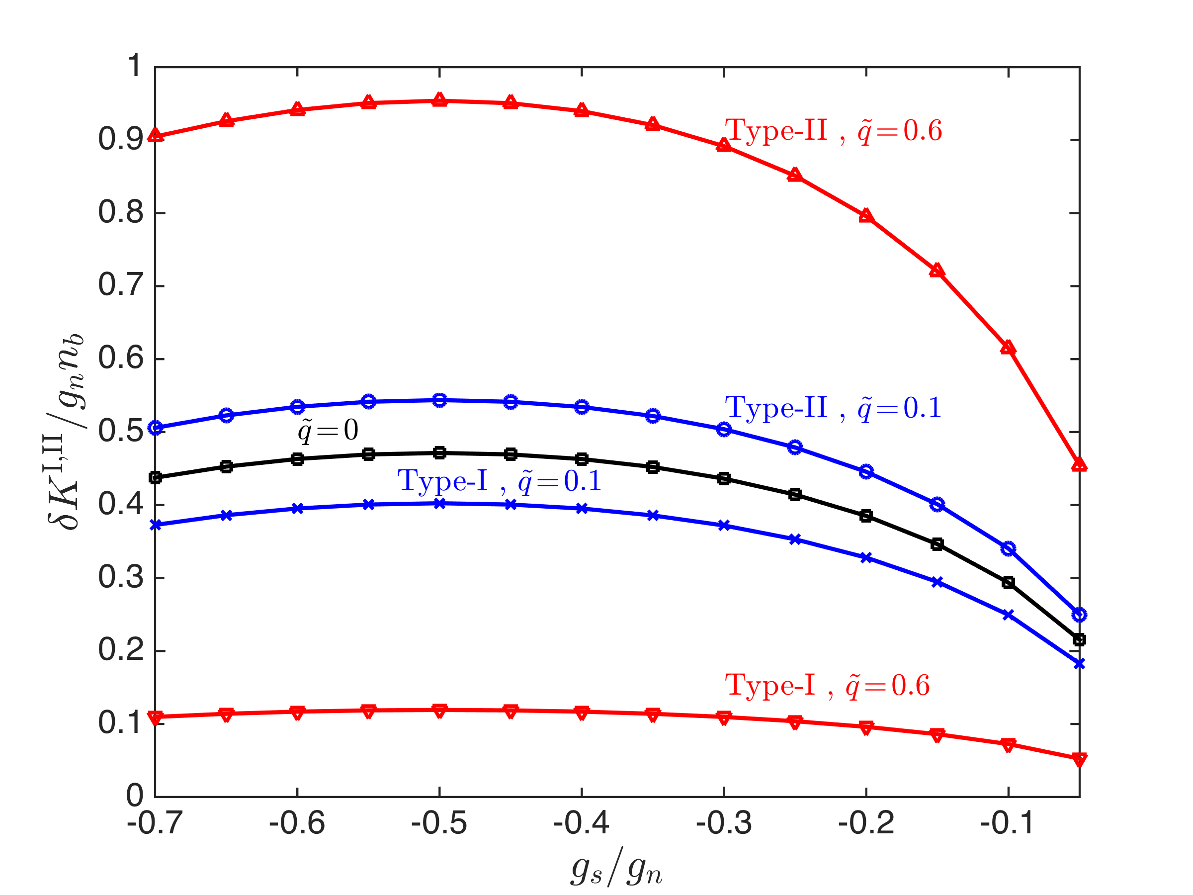
Figure 7: Numerical results of grand canonical energies for type-I and type-II FDSs at $\tilde{q}=0$, $\tilde{q}=0.1$ and $\tilde{q}=0.6$ (markers). Solid lines are guides to the eye. The soliton energy exhibits a non-monotonic behavior as a function of $g_{s}/g_{n}$ and the turning point occurs at the exactly solvable point $g_{s}/g_{n}=-0.5$. At $q=0$ (black squares), type-I and type-II FDSs are degenerate as for this case their states only differ by a $\textrm{SO}(3)$ spin rotation and a $\textrm{U}(1)$ gauge transformation Yu and Blakie (2021).

At $q=0$, type-I and type-II FDSs are degenerate and are connected by a $\textrm{SO}(3)$ spin-rotation Yu and Blakie (2021). At finite $q$ the magnetic field breaks the $\textrm{SO}(3)$ rotational symmetry and the degeneracy is lifted. We can characterize the degeneracy breaking using the soliton energy [see Eq. (34)] $\delta K^{\rm I,II}=K^{\rm I,II}-K_{g}$, where $K^{\rm I,II}=K[\psi^{\rm I,II}]$. We find that $\delta K^{\rm I}\leq\delta K^{\rm II}$ and the equality is reached only when $q=0$ (see Fig. 7).

V.4 Spin-singlet amplitudes

So far we have been focused on analyzing the structure of the order parameter $\mathbf{F}$ and the mass superfluid density $n$ which are the most relevant quantities to characterize FDSs. However, a complete description requires additional information. In general, the set $\{n,\mathbf{F},\alpha,\delta F^{2}_{z}\}$ provides a complete description of a spin-1 BEC, where

$$\alpha\equiv\psi^{2}_{0}-2\psi_{+1}\psi_{-1}$$ (51)

is the spin singlet amplitude and $\delta F^{2}_{z}\equiv\psi^{{\dagger}}S^{2}_{z}\psi=n_{+1}+n_{-1}$ couples to the quadratic Zeeman energy $q$ [see Eq. (1)]. The spin-singlet amplitude $\alpha$ is $\textrm{SO}(2)$ invariant and satisfies

$$|\mathbf{F}|^{2}+|\alpha|^{2}=n^{2}.$$ (52)

Let us consider variations that keep $\mathbf{F}$, $n$ and $\delta F^{2}_{z}$ unchanged. Such variations appear in the phase of $\alpha$. In the following we show that this particular phase change is nothing but the $\textrm{U}(1)$ phase variation which is directly related to the mass current

$$\mathbf{J}=\frac{\hbar}{2Mi}\left(\psi^{{\dagger}}\cdot\nabla\psi-\rm{H.c.}\right)$$ (53)

satisfying the continuity equation

$$\frac{\partial n}{\partial t}+\nabla\cdot\mathbf{J}=0.$$ (54)

For such variations, the deformed wavefunctions must have the form $\widetilde{\psi}_{i}=\psi_{i}e^{i\delta\theta_{i}(\mathbf{r})}$ and the corresponding transverse magnetization reads

$$\widetilde{F}_{\perp}=\sqrt{2}\left(\psi_{0}\psi^{*}_{+1}e^{i[\delta\theta_{0}(\mathbf{r})-\delta\theta_{+1}(\mathbf{r})]}+\psi^{*}_{0}\psi_{-1}e^{i[\delta\theta_{-1}(\mathbf{r})-\delta\theta_{0}(\mathbf{r})]}\right).$$ (55)

In order to keep invariant upon a global $\textrm{SO}(2)$ spin rotation, namely $\widetilde{F}_{\perp}=e^{i\phi}F_{\perp}$, the condition

$$\delta\theta_{0}(\mathbf{r})-\delta\theta_{+1}(\mathbf{r})=\delta\theta_{-1}(\mathbf{r})-\delta\theta_{0}(\mathbf{r})=\phi$$ (56)

must be satisfied, where $\phi$ is an arbitrary constant phase. Phase fluctuations satisfying Eq. (56) are captured by the spin-singlet, as $\widetilde{\alpha}=e^{2i\delta\theta_{0}(\mathbf{r})}\alpha=e^{2i[\delta\theta_{+1}(\mathbf{r})+\phi]}\alpha=e^{2i[\delta\theta_{-1}(\mathbf{r})-\phi]}\alpha$. It is also easy to see that $\delta\theta_{0}(\mathbf{r})$ or $\delta\theta_{\pm 1}(\mathbf{r})$ is an overall $\textrm{U}(1)$ phase variation and $\widetilde{\mathbf{J}}=\mathbf{J}+n\nabla\delta\theta_{0}(\mathbf{r})=\mathbf{J}+n\nabla\delta\theta_{\pm 1}(\mathbf{r})$. It is clear that a general phase variation of $\alpha$ does not necessarily have to be an overall $\textrm{U}(1)$ phase change.

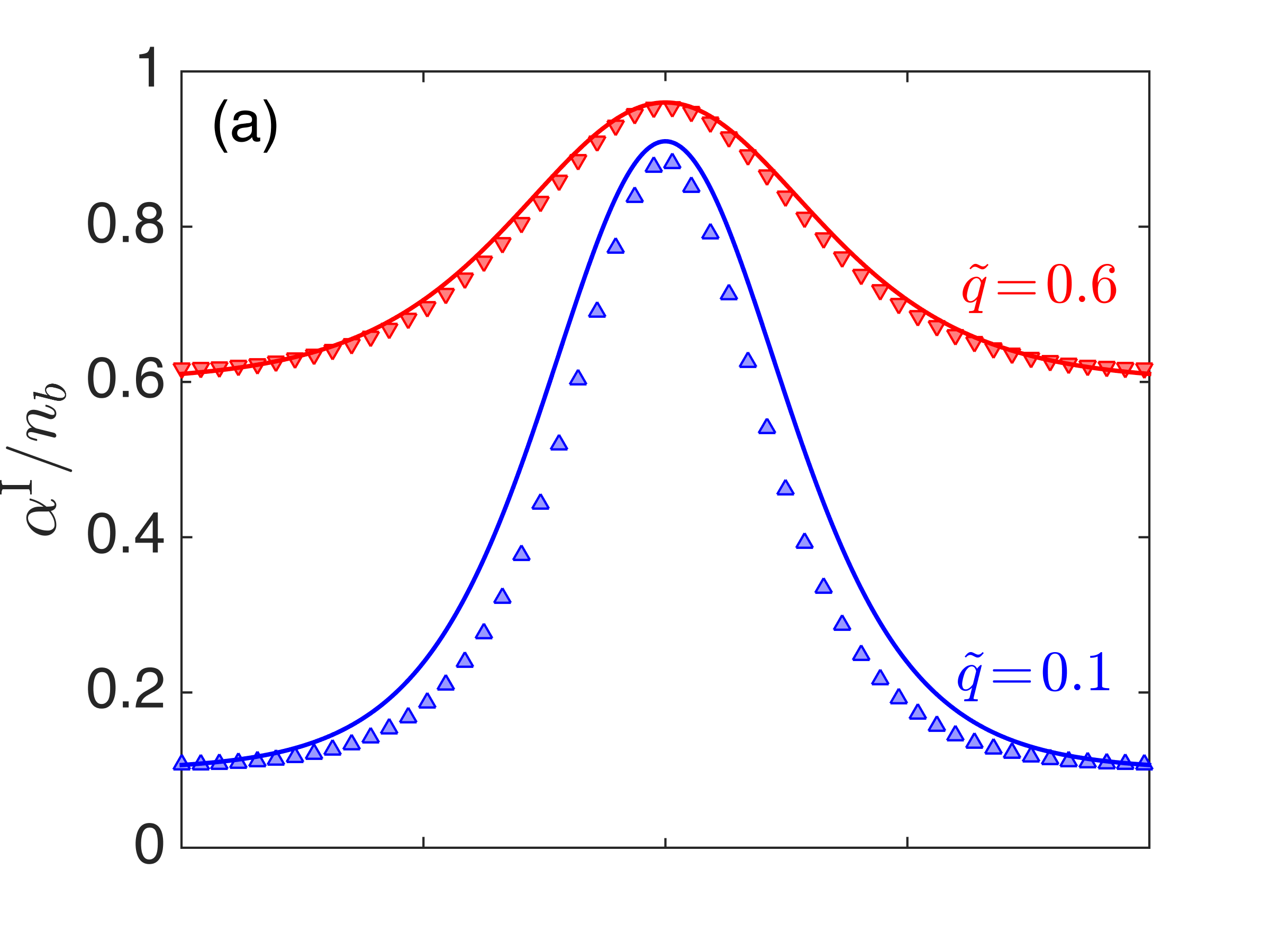
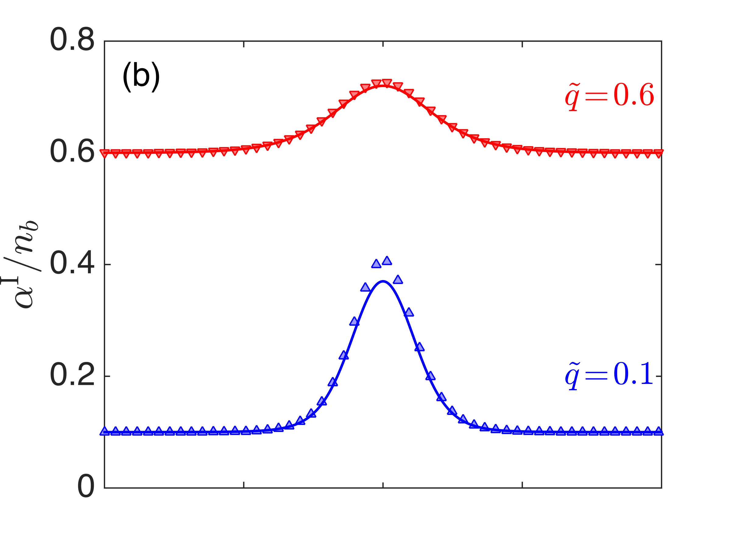
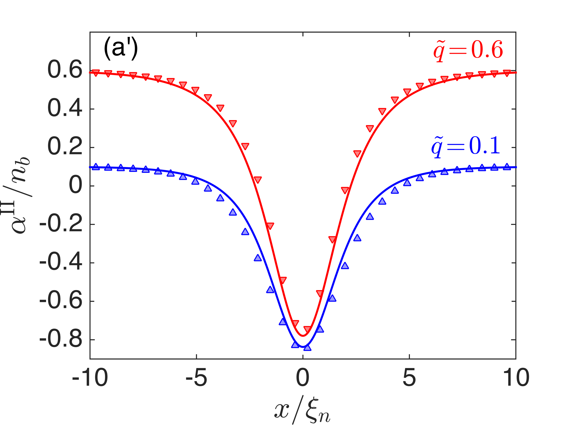
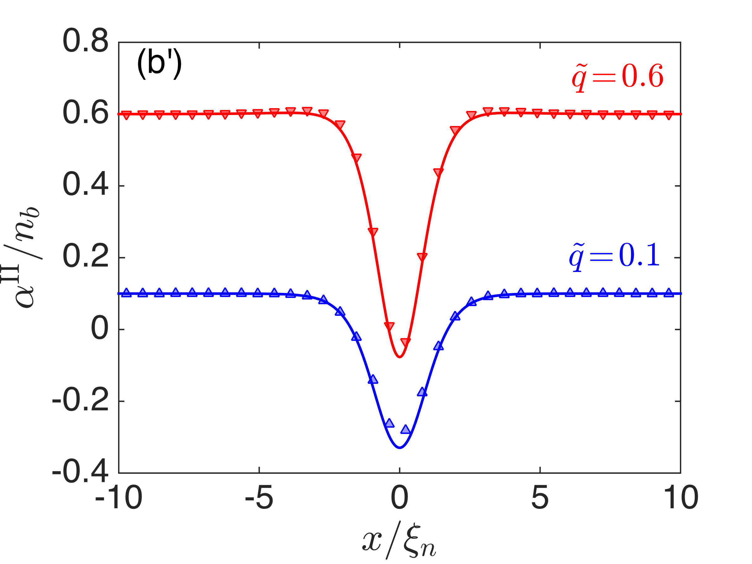
Figure 8: Analytical predictions (solid lines) and numerical results (markers) of the spin-singlet amplitude $\alpha$ for type-I [(a),(b)] and type-II [(a^′),(b^′)] FDSs at $\tilde{q}=0.1$ and $\tilde{q}=0.6$. (a) and (a^′) are for $g_{s}/g_{n}=-0.1$; (b) and (b^′) are for $g_{s}/g_{n}=-0.7$.

For FDSs, comparing to $n$, $\mathbf{F}$ and $\delta F^{2}_{z}$, the spin-singlet amplitude $\alpha$ is a more appealing quantity to distinguish type-I from type-II FDSs as it shows a hump or a dip depending on the type (Fig. 8). The measurement of $\alpha$ is in the scope of the current spin-1 BECs experiments Kunkel et al. (2019).

VI Nematic structure

It is sometimes useful to formulate the spin-1 BEC dynamics in terms of physical observables. The hydrodynamic formulation of the GPEs Eqs. (2) and (3) serves this purpose and provides a complete description of the condensate dynamics Yukawa and Ueda (2012). Such a description naturally involves nematic tensors and the corresponding currents. Although $n$, $\mathbf{F}$, $\alpha$ and $\delta F^{2}_{z}$ together also fully describe a spin-1 BEC, it is not anticipated that the construction of self-contained closed dynamical equations with these variables is achievable. In this section, we explore nematic structure of FDSs.

VI.1 General formulation

The magnetization continuity equation reads

$$\frac{\partial F_{i}}{\partial t}+\nabla\cdot J^{F}_{i}=K_{iz},$$ (57)

where the spin current density

$$J^{F}_{i}=\frac{\hbar}{2Mi}\left(\psi^{{\dagger}}S_{i}\nabla\psi-\nabla\psi^{{\dagger}}S_{i}\psi\right),$$ (58)

and the source term (or the internal current density)

$$K_{iz}=\frac{2q}{\hbar}\sum_{k}\epsilon_{izk}N_{zk}.$$ (59)

Explicitly, the components are $K_{xz}=-(2q/\hbar)N_{zy}$, $K_{yz}=(2q/\hbar)N_{zx}$ and $K_{zz}=0$, where $N_{ij}$ is the nematic (or quadrupolar) tensor density

$$N_{ij}=\psi^{{\dagger}}\hat{N}_{ij}\psi$$ (60)

with $\hat{N}_{ij}=(S_{i}S_{j}+S_{j}S_{i})/2$ and $i,j\in\{x,y,z\}$. The nematic tensor serves as an order parameter if $F_{i}=0$ Gramsbergen et al. (1986); Symes and Blakie (2017) and describes spin fluctuations in the ferromagnetic phase. It is easy to recognize that $N_{zz}=\delta F^{2}_{z}$.

The nematic continuity equation reads

$$\frac{\partial N_{ij}}{\partial t}+\nabla\cdot J^{N}_{ij}=W_{ij}+Q_{ijz},$$ (61)

where the nematic current density

$$J^{N}_{ij}=\frac{\hbar}{2Mi}\left(\psi^{{\dagger}}\hat{N}_{ij}\nabla\psi-\nabla\psi^{{\dagger}}\hat{N}_{ij}\psi\right),$$ (62)

and the source terms (or the internal current densities)

$$W_{ij} =\frac{g_{s}}{\hbar}\sum_{l,k}F_{l}\left(\epsilon_{ilk}N_{kj}+\epsilon_{jlk}N_{ki}\right),$$ (63)

$$Q_{ijz} =\frac{q}{2\hbar}\sum_{k}F_{k}\left(\epsilon_{izk}\delta_{zj}+\epsilon_{jzk}\delta_{zi}\right).$$ (64)

Since ${\rm Tr}{N}=\sum_{i}{N_{ii}}=n$, the total density continuity equation (54) can be obtained by taking the trace of Eq. (61). It is easy to see that ${\rm Tr}{W}=0$ and $Q_{iiz}=0$. Also $Q_{xzz}=Q_{zxz}=-(q/2\hbar)F_{y}$ and $Q_{yzz}=Q_{zyz}=(q/2\hbar)F_{x}$, and all the other components are zero. Hence $Q_{ijz}$ does not contain new information. The continuity equations (54), (57), (61) and the equation of motion of the mass current $\mathbf{J}$ (Euler equation) together provide a complete description of spin-1 BECs dynamics Yukawa and Ueda (2012).

Except the total number density $n$ and the total number current $\mathbf{J}$, the expressions of other densities and currents vary when applying spin-rotations. Hence it is useful to construct rotationally invariant quantities to reveal intrinsic currents. Here we find that the densities

$$F\equiv\left[\sum_{i}\left(F_{i}\right)^{2}\right]^{1/2},\quad{\cal N}\equiv\left[\sum_{ij}\left(N_{ij}\right)^{2}\right]^{1/2}$$ (65)

and the current densities

$${\cal J}_{F}\equiv \left[\sum_{i}\left(J^{F}_{i}\right)^{2}\right]^{1/2},$$

$${\cal J}_{N}\equiv \left[\sum_{ij}\left(J^{N}_{ij}\right)^{2}\right]^{1/2},$$

$${\cal W}\equiv \left[\sum_{ij}\left(W_{ij}\right)^{2}\right]^{1/2}$$ (66)

are invariant under $\textrm{SO}(3)$ spin-rotations. The source terms

$${\cal Q}\equiv\left[\sum_{ij}\left(Q_{ijz}\right)^{2}\right]^{1/2},\quad{\cal K}\equiv\left[\sum_{i}\left(K_{iz}\right)^{2}\right]^{1/2}$$ (67)

only appear in the equation of motion when $q\neq 0$, and are $\textrm{SO}(2)$ rotationally invariant.

VI.2 Nematic structure of FDSs

At the exactly solvable point $g_{s}=-g_{n}/2$, the invariant nematic densities read

$$({\cal N}^{\rm I,II})^{2} =\frac{1}{4}\left[4\left(n_{b}-\frac{g_{n}n_{b}\mp q}{g_{n}\cosh\left(\frac{x}{\ell^{\rm I,II}_{q}}\right)+g_{n}}\right)^{2}\right.$$

$$\left.+\left(n_{b}\mp\frac{q}{g_{n}}\right)^{2}\tanh^{4}\left(\frac{x}{2\ell^{\rm I,II}_{q}}\right)+\left(n_{b}\pm\frac{q}{g_{n}}\right)^{2}\right],$$

where the upper (lower) sign in front of $q$ specifies the type-I (type-II) FDS. Away from the exactly solvable point, the ansatzes also describe well the nematic densities in a wide range parameter regime (Fig.9).

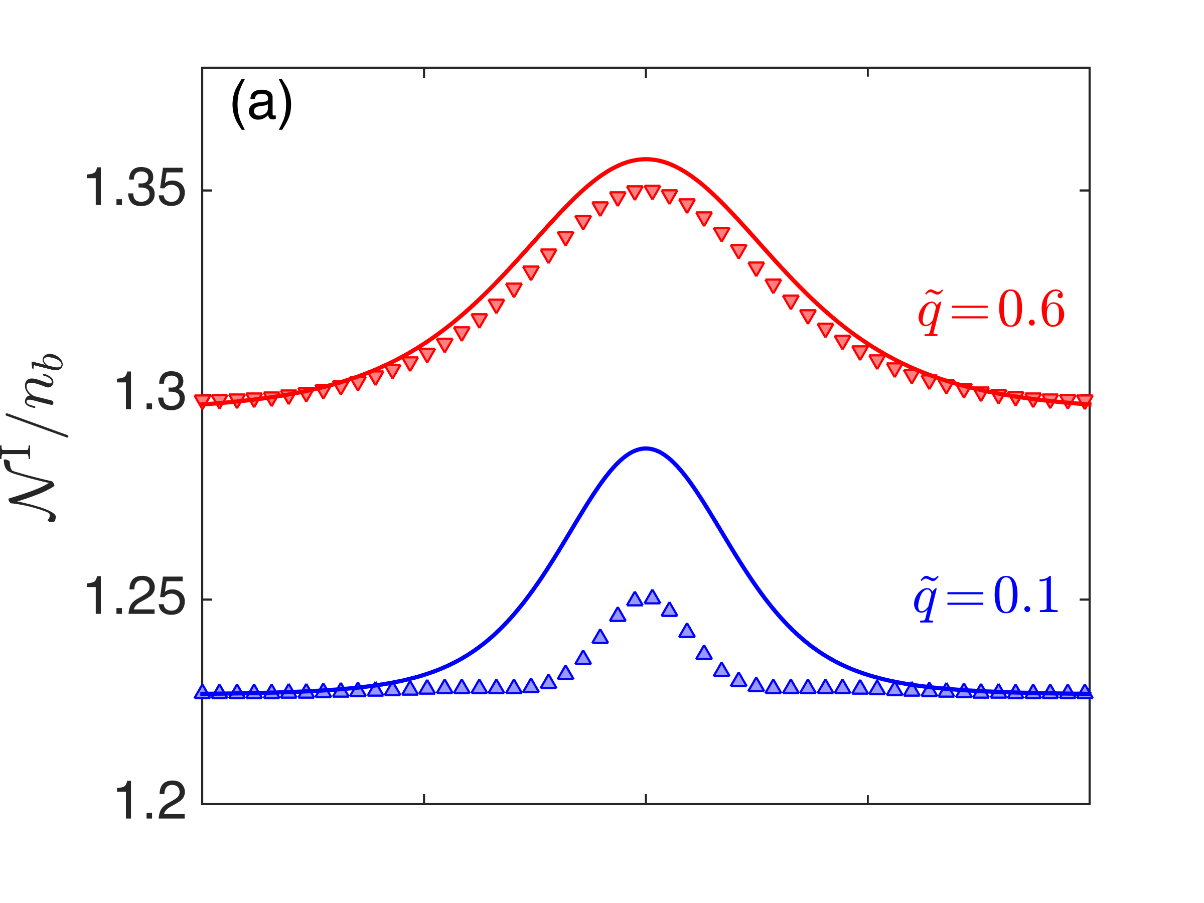
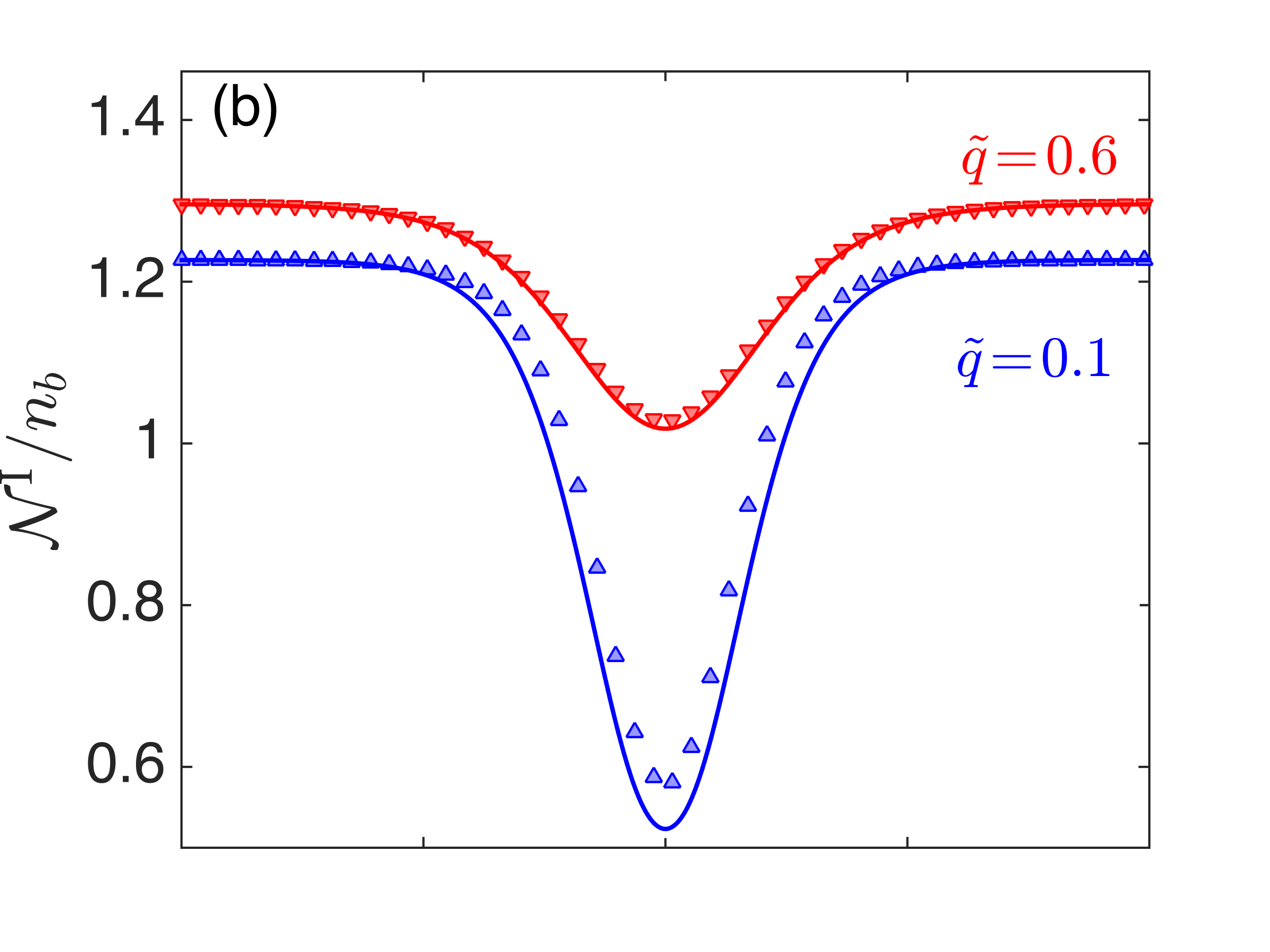
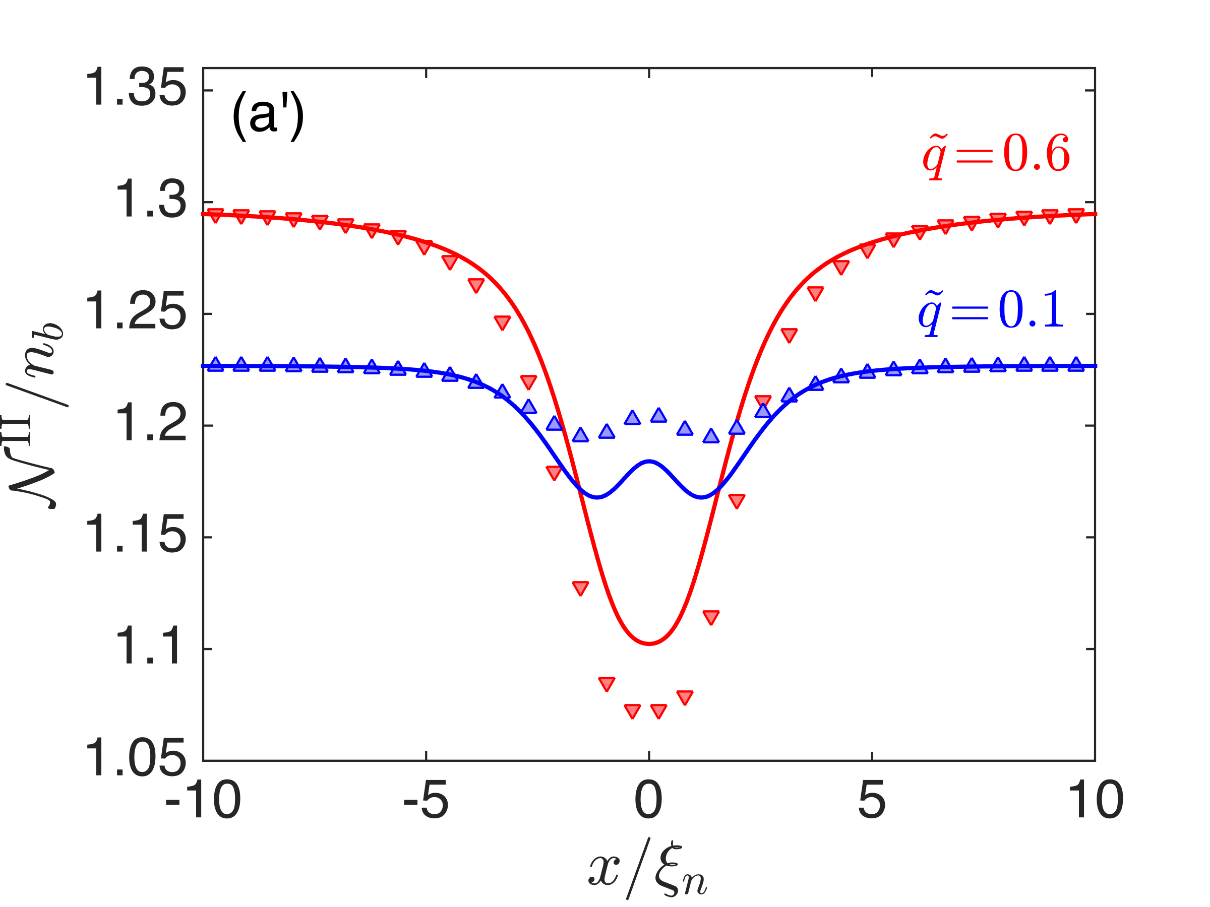
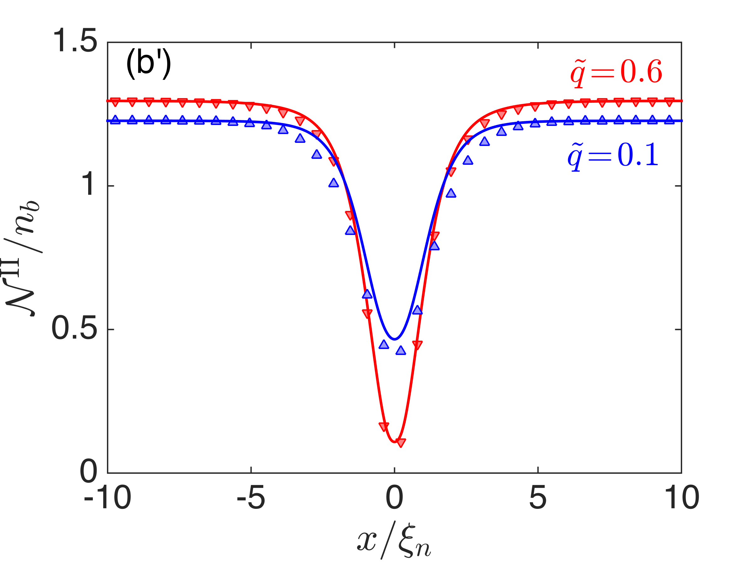
Figure 9: Analytical predictions (solid lines) and numerical results (markers) of the rotationally invariant nematic density ${\cal N}$ for type-I [(a),(b)] and type-II [(a^′),(b^′)] FDSs at $\tilde{q}=0.1$ and $\tilde{q}=0.6$. (a) and (a^′) are for $g_{s}/g_{n}=-0.1$; (b) and (b^′) are for $g_{s}/g_{n}=-0.7$.

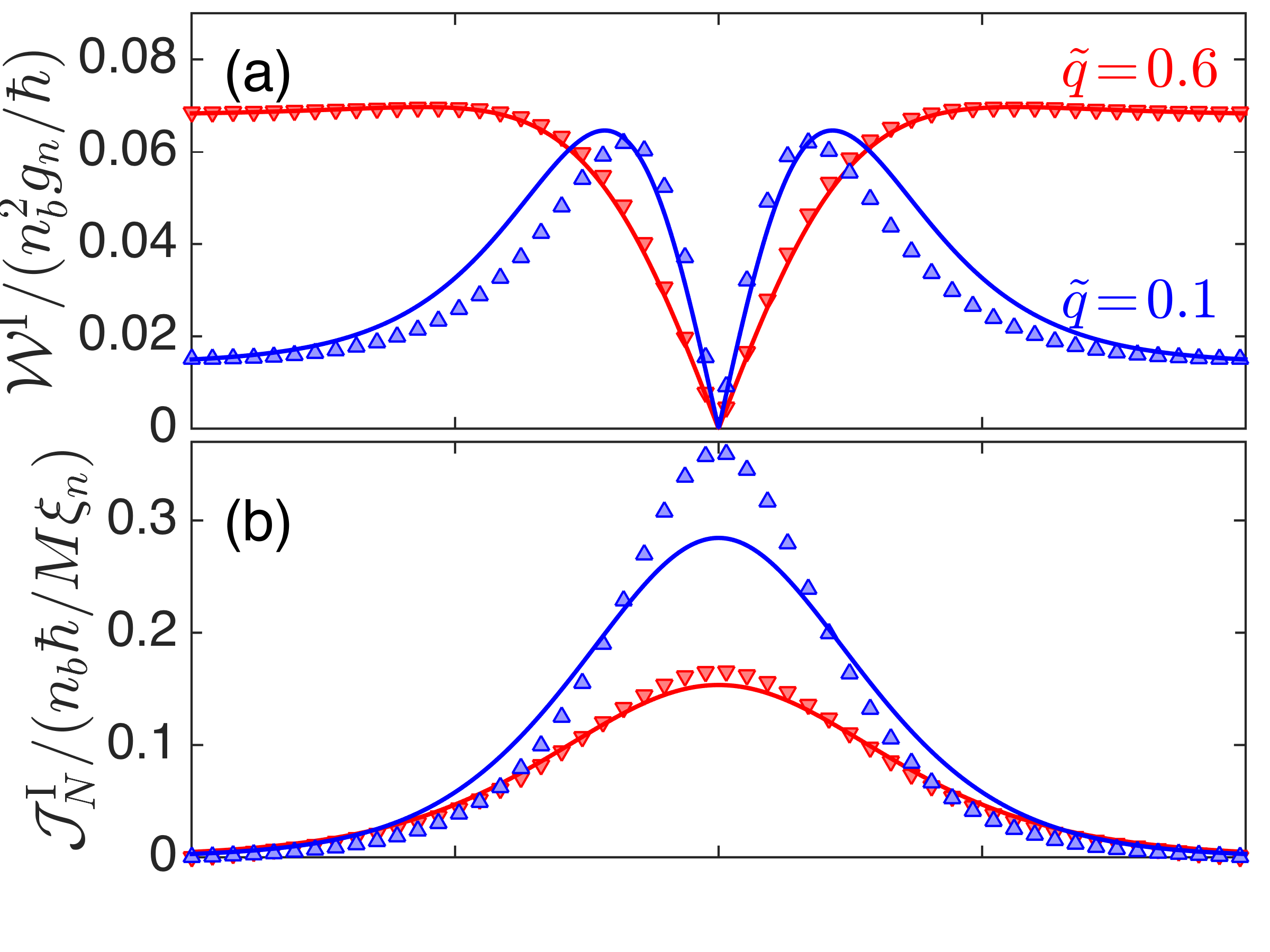
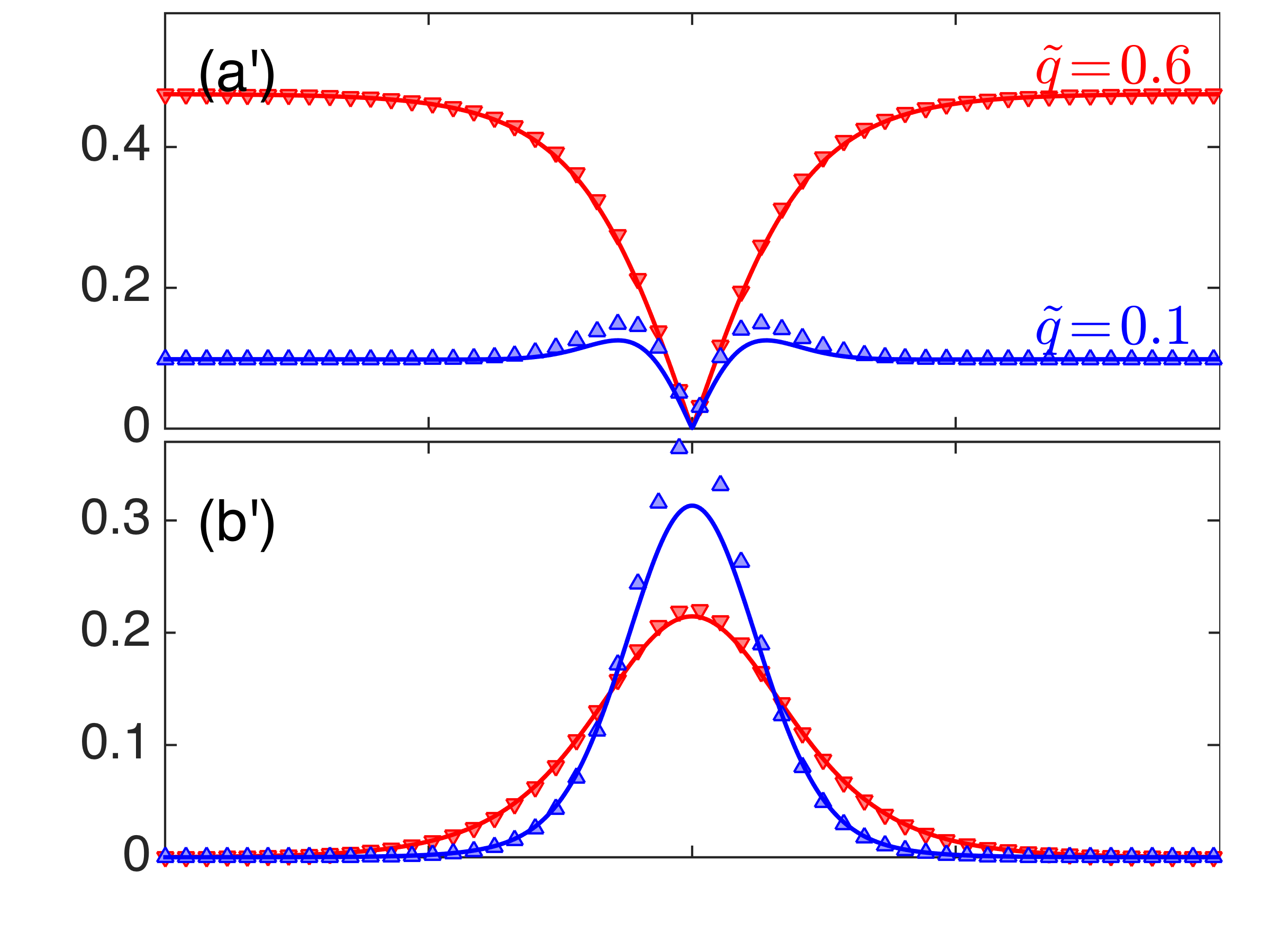
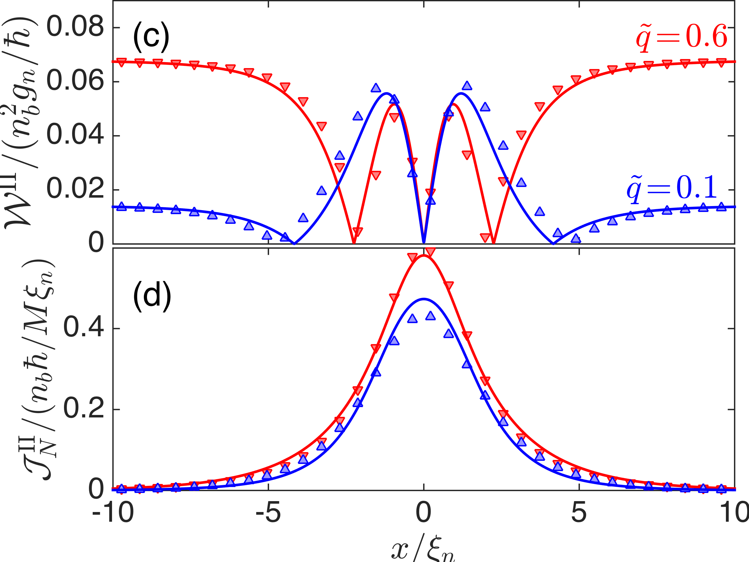
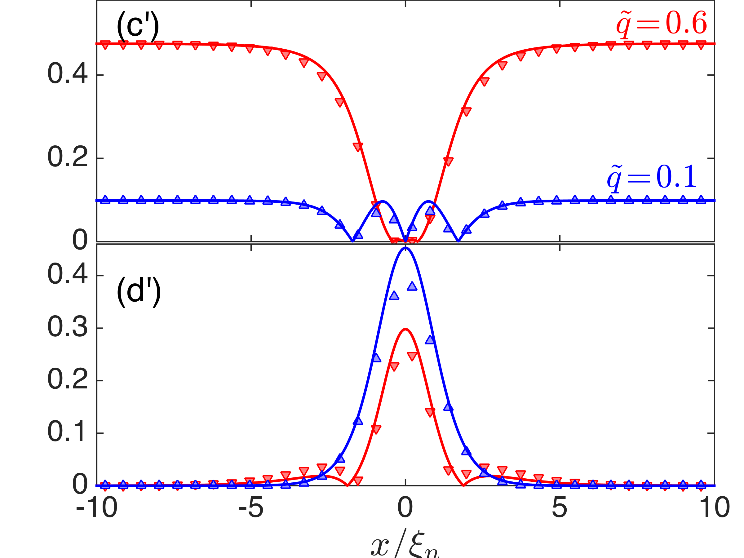
Figure 10: Profiles of invariant internal currents of FDSs. Analytical predictions (solid lines) and numerical results (markers) are shown at $\tilde{q}=0.1$ (blue) and $\tilde{q}=0.6$ (red). (a), (b), (c) and (d) are for $g_{s}/g_{n}=-0.1$; (a^′), (b^′), (c^′) and (d^′) are for $g_{s}/g_{n}=-0.7$. The $y$-axis labels of (a^′), (b^′), (c^′) and (d^′) are the same as the $y$-axis labels of (a), (b), (c) and (d).

Figure 10 shows the profiles of the invariant internal current densities. At the exactly solvable point,

$$({\cal J}^{\rm I,II}_{N})^{2} =\frac{\hbar^{2}(g_{n}^{2}n_{b}^{2}-q^{2})}{32(\ell^{\rm I,II}_{q})^{2}M^{2}g^{2}_{n}}\operatorname{sech}^{4}\left(\frac{x}{2\ell^{\rm I,II}_{q}}\right),$$ (69)

$$({\cal W}^{\rm I,II})^{2} =\frac{g^{2}_{n}n^{2}_{b}-q^{2}}{8g_{n}^{2}\hbar^{2}}\tanh^{2}\left(\frac{x}{2\ell^{\rm I,II}_{q}}\right)\times$$ (70)

$$\operatorname{sech}^{4}\left(\frac{x}{2\ell^{\rm I,II}_{q}}\right)\left[g_{n}n_{b}\pm q\cosh\left(\frac{x}{\ell^{\rm I,II}_{q}}\right)\right]^{2},$$

here the plus sign and minus sign in front of $q$ specify type-I and type-II FDSs respectively.

VII Conclusion and discussion

We have studied the $\mathbb{Z}_{2}$ topological defects in the easy-plane phase of a ferromagnetic spin-1 BEC. We propose analytical ansatzes to describe ferrodark solitons (FDSs) which are the defects in the magnetic order. The ansatzes reduce to the exact solutions at the exactly solvable point and show good agreement with numerical results over the whole easy-plane phase. The width of type-I FDSs is captured by a single scale while the core structure of type-II FDSs require two scales. Moreover, exact dark-dark-dark (DDD) vector solitons, which are the $\mathbb{Z}_{2}$ defects in the mass superfluid order, are also presented. FDSs are expected to play an important role in late time dynamics of 1D quenches Prüfer et al. (2018); Schmied et al. (2019b) and equilibrium properties at finite temperature Prüfer et al. (2022).

Experimental advances now allow plane-confined BECs with flat-bottom traps Chomaz et al. (2015); Gauthier et al. (2016) and the measurement of transverse magnetic structures by the nondestructive imaging method  Higbie et al. (2005); Kunkel et al. (2019), opening the possibility for detailed experimental investigations of FDSs. The so-called magnetic phase imprinting method, which has been used to experimentally create pairs of magnetic solitons Farolfi et al. (2020); Chai et al. (2020), could be a suitable method to create FDSs in a ferromagnetic spin-1 BEC. Very recently, the easy-plane phase of a homogeneous ferromagnetic spin-1 BEC has been prepared in a flat-bottom trapped quasi-one dimensional system Prüfer et al. (2022). The magnetic phase imprinting method applies circularly polarized light to imprint a phase shift of $\pm\pi$ onto two $m=\pm 1$ hyperfine components on half the system by using a magnetic shadow Farolfi et al. (2020); Chai et al. (2020). This hence realizes a $\pi$ spin rotation of the transverse magnetization of half of the system, seeding the key ingredient of a single FDS.

In this paper we focus on kinks/topological solitons in the easy-plane phase of ferromagnetic spin-1 BECs. A FDS is a $\mathbb{Z}_{2}$ topological defect which interpolates between oppositely magnetized domains. From another perspective, it could be useful to view FDSs as members of the soliton family in spin-1 BECs and compare them with other nonlinear waves. Here we give a brief summary of the main focus of recent soliton studies in spin-1 BECs. The list is incomplete, for instance, solitons in systems with optical lattices and dipole-dipole interactions Xie et al. (2004); Li et al. (2005) are not included. Also we only consider systems with the finite background density, i.e., the positive density-dependent interaction strength. According to the terminologies, there are mainly two varieties. i) Vector solitons: each component has either dark or bright soliton structure  Nistazakis et al. (2008); Busch and Anglin (2001); Liu et al. (2009); Bersano et al. (2018); Lannig et al. (2020); Katsimiga et al. (2021) (Ref. Katsimiga et al. (2021) discusses two-dimensional extensions of such excitations, i.e., vortex-bright structures). Various vector solitons in a 1D harmonically trapped spin-1 system have been recently summarized in Ref. Katsimiga et al. (2021). Vector solitons may or may not correspond to topological structures in the order parameter. There are two interesting examples which are topological. One is the dark-dark-dark vector soliton in ferromagnetic BECs which is the topological defect in the mass superfluid order as discussed in Sec. IV. Another one is the bright-dark-bright vector soliton in an anti-ferromagnetic BEC which manifests itself as a domain wall in the spin director field (the order parameter) Kang et al. (2019). ii) Magnetic solitons: this soliton was initially introduced in miscible two-component BECs Qu et al. (2016) and can be embedded into an anti-ferromagnetic spin-1 BEC in the absence of a magnetic field Farolfi et al. (2020); Chai et al. (2020, 2021). One important aspect of this soliton is that it is an analytical solution which is beyond the Manakov limit. The solution is obtained with the constant density approximation which works well for weak spin-dependent coupling $g_{s}$. In the context of two-component BECs, it emphasizes that there is no bright or dark soliton structure in the components, while the pseudo magnetization $F_{z}$ shows a bright soliton structure. When embedding into anti-ferromagnetic spin-1 BECs, its configuration varies under $\textrm{SO}(3)$ spin-rotations Chai et al. (2021) as what happens for FDSs at $q\rightarrow 0$ limit Yu and Blakie (2021). The magnetic soliton is not a topological soliton as there is no invariant topological charge associated with it (neither in its original two-component formulation nor in its realizations in an anti-ferromagnetic spin-1 BEC). FDSs do not belong to vector solitons, as not all the components of FDSs have bright or dark soliton structure. The topological nature of FDSs also clearly distinguish themselves from magnetic solitons. Moreover, exact solutions for FDSs are available at a strong spin-dependent interaction coupling ($g_{s}/g_{n}=-1/2$) Yu and Blakie (2021, 2022) which is far beyond the Manakov limit ($g_{s}=0$ in the context of spin-1 BECs).

FDSs are Ising type magnetic domain walls. A natural question is that whether Bloch type and Néel type magnetic domain walls could exist in the easy-plane phase. A Néel type-like domain wall has been investigated numerically in a trapped 1D ferromagnetic BECs at $q=0$ Zhang et al. (2007), which might be related to the wall defects appearing transiently in early quench dynamics from unmagnetized or partially magnetized states Zhang et al. (2005); Saito and Ueda (2005). However it is not clear whether the trap potential plays the key role to sustain this structure. Searching for Bloch type and Néel type magnetic domain walls in the easy-plane phase of ferromagnetic BECs deserves future investigations.

So far we only consider excitations from a uniform ground state. In immiscible condensates, domain walls are also referred to as the interfaces between the spatially separated components of the condensate, examples are density (or pseudo magnetization $F_{z}$) domain walls in immiscible binary BECs Ao and Chui (1998); Coen and Haelterman (2001); Chai et al. (2022); foo (b), and magnetic domain walls in ferromagnetic spin-1 BECs for a negative quadratic Zeeman shift $q<0$ Takeuchi (2022).

References

- Ho (1998) Tin-Lun Ho, “Spinor Bose condensates in optical traps,” Phys. Rev. Lett. 81, 742 (1998).
- Ohmi and Machida (1998) Tetsuo Ohmi and Kazushige Machida, “Bose-Einstein condensation with internal degrees of freedom in alkali atom gases,” J. Phys. Soc. Jpn 67, 1822 (1998).
- Stenger et al. (1998) J. Stenger, S. Inouye, D. M. Stamper-Kurn, H. J. Miesner, A. P. Chikkatur, and W. Ketterle, “Spin domains in ground-state Bose–Einstein condensates,” Nature 396, 345 (1998).
- Sadler et al. (2006) L. E. Sadler, J. M. Higbie, S. R. Leslie, M. Vengalattore, and D. M. Stamper-Kurn, “Spontaneous symmetry breaking in a quenched ferromagnetic spinor Bose–Einstein condensate,” Nature 443, 312 (2006).
- Stamper-Kurn and Ueda (2013) Dan M. Stamper-Kurn and Masahito Ueda, “Spinor Bose gases: Symmetries, magnetism, and quantum dynamics,” Rev. Mod. Phys. 85, 1191 (2013).
- Kawaguchi and Ueda (2012) Yuki Kawaguchi and Masahito Ueda, “Spinor Bose–Einstein condensates,” Phys. Rep. 520, 253 (2012), spinor Bose–Einstein condensates.
- James and Lamacraft (2011) A. J. A. James and A. Lamacraft, “Phase diagram of two-dimensional polar condensates in a magnetic field,” Phys. Rev. Lett. 106, 140402 (2011).
- Kobayashi (2019) Michikazu Kobayashi, “Berezinskii–Kosterlitz–Thouless transition of spin-1 spinor Bose gases in the presence of the quadratic zeeman effect,” J. Phys. Soc. Jpn 88, 094001 (2019).
- Saito et al. (2007a) Hiroki Saito, Yuki Kawaguchi, and Masahito Ueda, “Kibble-Zurek mechanism in a quenched ferromagnetic Bose-Einstein condensate,” Phys. Rev. A 76, 043613 (2007a).
- Damski and Zurek (2007) Bogdan Damski and Wojciech H. Zurek, “Dynamics of a quantum phase transition in a ferromagnetic Bose-Einstein condensate,” Phys. Rev. Lett. 99, 130402 (2007).
- Lamacraft (2007) Austen Lamacraft, “Quantum quenches in a spinor condensate,” Phys. Rev. Lett. 98, 160404 (2007).
- Mukerjee et al. (2007) Subroto Mukerjee, Cenke Xu, and J. E. Moore, “Dynamical models and the phase ordering kinetics of the spinor condensate,” Phys. Rev. B 76, 104519 (2007).
- Williamson and Blakie (2016a) Lewis A. Williamson and P. B. Blakie, “Universal coarsening dynamics of a quenched ferromagnetic spin-1 condensate,” Phys. Rev. Lett. 116, 025301 (2016a).
- Williamson and Blakie (2017) L. A. Williamson and P. B. Blakie, “Coarsening dynamics of an isotropic ferromagnetic superfluid,” Phys. Rev. Lett. 119, 255301 (2017).
- Symes and Blakie (2017) L. M. Symes and P. B. Blakie, “Nematic ordering dynamics of an antiferromagnetic spin-1 condensate,” Phys. Rev. A 96, 013602 (2017).
- Schmied et al. (2019a) C.-M. Schmied, T. Gasenzer, and P. B. Blakie, “Violation of single-length-scaling dynamics via spin vortices in an isolated spin-1 Bose gas,” Phys. Rev. A 100, 033603 (2019a).
- Bourges and Blakie (2017) Andréane Bourges and P. B. Blakie, “Different growth rates for spin and superfluid order in a quenched spinor condensate,” Phys. Rev. A 95, 023616 (2017).
- Barnett et al. (2011) Ryan Barnett, Anatoli Polkovnikov, and Mukund Vengalattore, “Prethermalization in quenched spinor condensates,” Phys. Rev. A 84, 023606 (2011).
- Fujimoto et al. (2019) Kazuya Fujimoto, Ryusuke Hamazaki, and Masahito Ueda, “Flemish strings of magnetic solitons and a nonthermal fixed point in a one-dimensional antiferromagnetic spin-1 Bose gas,” Phys. Rev. Lett. 122, 173001 (2019).
- Williamson and Blakie (2016b) Lewis A. Williamson and P. B. Blakie, “Dynamics of polar-core spin vortices in a ferromagnetic spin-1 Bose-Einstein condensate,” Phys. Rev. A 94, 063615 (2016b).
- Turner (2009) Ari M. Turner, “Mass of a spin vortex in a Bose-Einstein condensate,” Phys. Rev. Lett. 103, 080603 (2009).
- Yu and Blakie (2021) Xiaoquan Yu and P. B. Blakie, “Dark-soliton-like magnetic domain walls in a two-dimensional ferromagnetic superfluid,” Phys. Rev. Research 3, 023043 (2021).
- Yu and Blakie (2022) Xiaoquan Yu and P. B. Blakie, “Propagating ferrodark solitons in a superfluid: Exact solutions and anomalous dynamics,” Phys. Rev. Lett. 128, 125301 (2022).
- Saito et al. (2007b) Hiroki Saito, Yuki Kawaguchi, and Masahito Ueda, “Topological defect formation in a quenched ferromagnetic Bose-Einstein condensates,” Phys. Rev. A 75, 013621 (2007b).
- Saito and Ueda (2005) Hiroki Saito and Masahito Ueda, “Spontaneous magnetization and structure formation in a spin-1 ferromagnetic Bose-Einstein condensate,” Phys. Rev. A 72, 023610 (2005).
- Prüfer et al. (2018) Maximilian Prüfer, Philipp Kunkel, Helmut Strobel, Stefan Lannig, Daniel Linnemann, Christian-Marcel Schmied, Jürgen Berges, Thomas Gasenzer, and Markus K. Oberthaler, “Observation of universal dynamics in a spinor Bose gas far from equilibrium,” Nature 563, 217 (2018).
- Schmied et al. (2019b) Christian-Marcel Schmied, Maximilian Prüfer, Markus K. Oberthaler, and Thomas Gasenzer, “Bidirectional universal dynamics in a spinor bose gas close to a nonthermal fixed point,” Phys. Rev. A 99, 033611 (2019b).
- Mizushima et al. (2002) T. Mizushima, K. Machida, and T. Kita, “Mermin-ho vortex in ferromagnetic spinor bose-einstein condensates,” Phys. Rev. Lett. 89, 030401 (2002).
- Kudo and Kawaguchi (2015) Kazue Kudo and Yuki Kawaguchi, “Coarsening dynamics driven by vortex-antivortex annihilation in ferromagnetic Bose-Einstein condensates,” Phys. Rev. A 91, 053609 (2015).
- Zhang et al. (2003) Wenxian Zhang, Su Yi, and Li You, “Mean field ground state of a spin-1 condensate in a magnetic field,” New Journal of Physics 5, 77 (2003).
- Huh et al. (2020) SeungJung Huh, Kyungtae Kim, Kiryang Kwon, and Jae-yoon Choi, “Observation of a strongly ferromagnetic spinor Bose-Einstein condensate,” Phys. Rev. Research 2, 033471 (2020).
- Katsimiga et al. (2021) G C Katsimiga, S I Mistakidis, P Schmelcher, and P G Kevrekidis, “Phase diagram, stability and magnetic properties of nonlinear excitations in spinor Bose–Einstein condensates,” New J. Phys. 23, 013015 (2021).
- foo (a) No convergent DDD soliton solution is found for .
- Lim and Bao (2008) Fong Yin Lim and Weizhu Bao, “Numerical methods for computing the ground state of spin-1 Bose-Einstein condensates in a uniform magnetic field,” Phys. Rev. E 78, 066704 (2008).
- Bao and Lim (2008) Weizhu Bao and Fong Yin Lim, “Computing ground states of spin-1 Bose–Einstein condensates by the normalized gradient flow,” SIAM J. Sci. Comput. 30, 1925 (2008).
- Kunkel et al. (2019) Philipp Kunkel, Maximilian Prüfer, Stefan Lannig, Rodrigo Rosa-Medina, Alexis Bonnin, Martin Gärttner, Helmut Strobel, and Markus K. Oberthaler, “Simultaneous readout of noncommuting collective spin observables beyond the standard quantum limit,” Phys. Rev. Lett. 123, 063603 (2019).
- Yukawa and Ueda (2012) Emi Yukawa and Masahito Ueda, “Hydrodynamic description of spin-1 Bose-Einstein condensates,” Phys. Rev. A 86, 063614 (2012).
- Gramsbergen et al. (1986) Egbert F. Gramsbergen, Lech Longa, and Wim H. de Jeu, “Landau theory of the nematic-isotropic phase transition,” Phys. Rep. 135, 195 (1986).
- Prüfer et al. (2022) Maximilian Prüfer, Daniel Spitz, Stefan Lannig, Helmut Strobel, Jürgen Berges, and Markus K. Oberthaler, “Condensation and thermalization of an easy-plane ferromagnet in a spinor Bose gas,” arXiv e-prints , arXiv:2205.06188 (2022), arXiv:2205.06188 [cond-mat.quant-gas] .
- Chomaz et al. (2015) Lauriane Chomaz, Laura Corman, Tom Bienaimé, Rémi Desbuquois, Christof Weitenberg, Sylvain Nascimbène, Jérôme Beugnon, and Jean Dalibard, “Emergence of coherence via transverse condensation in a uniform quasi-two-dimensional Bose gas,” Nat. Commun. 6 (2015).
- Gauthier et al. (2016) G. Gauthier, I. Lenton, N. McKay Parry, M. Baker, M. J. Davis, H. Rubinsztein-Dunlop, and T. W. Neely, “Direct imaging of a digital-micromirror device for configurable microscopic optical potentials,” Optica 3, 1136 (2016).
- Higbie et al. (2005) J. M. Higbie, L. E. Sadler, S. Inouye, A. P. Chikkatur, S. R. Leslie, K. L. Moore, V. Savalli, and D. M. Stamper-Kurn, “Direct nondestructive imaging of magnetization in a spin-1 Bose-Einstein gas,” Phys. Rev. Lett. 95, 050401 (2005).
- Farolfi et al. (2020) A. Farolfi, D. Trypogeorgos, C. Mordini, G. Lamporesi, and G. Ferrari, “Observation of magnetic solitons in two-component Bose-Einstein condensates,” Phys. Rev. Lett. 125, 030401 (2020).
- Chai et al. (2020) X. Chai, D. Lao, Kazuya Fujimoto, Ryusuke Hamazaki, Masahito Ueda, and C. Raman, “Magnetic solitons in a spin-1 Bose-Einstein condensate,” Phys. Rev. Lett. 125, 030402 (2020).
- Xie et al. (2004) Zheng-Wei Xie, Weiping Zhang, S. T. Chui, and W. M. Liu, “Magnetic solitons of spinor Bose-Einstein condensates in an optical lattice,” Phys. Rev. A 69, 053609 (2004).
- Li et al. (2005) Z. D. Li, P. B. He, L. Li, J. Q. Liang, and W. M. Liu, “Magnetic soliton and soliton collisions of spinor Bose-Einstein condensates in an optical lattice,” Phys. Rev. A 71, 053611 (2005).
- Nistazakis et al. (2008) H. E. Nistazakis, D. J. Frantzeskakis, P. G. Kevrekidis, B. A. Malomed, and R. Carretero-González, “Bright-dark soliton complexes in spinor Bose-Einstein condensates,” Phys. Rev. A 77, 033612 (2008).
- Busch and Anglin (2001) Th. Busch and J. R. Anglin, “Dark-bright solitons in inhomogeneous Bose-Einstein condensates,” Phys. Rev. Lett. 87, 010401 (2001).
- Liu et al. (2009) Xunxu Liu, Han Pu, Bo Xiong, W. M. Liu, and Jiangbin Gong, “Formation and transformation of vector solitons in two-species Bose-Einstein condensates with a tunable interaction,” Phys. Rev. A 79, 013423 (2009).
- Bersano et al. (2018) T. M. Bersano, V. Gokhroo, M. A. Khamehchi, J. D’Ambroise, D. J. Frantzeskakis, P. Engels, and P. G. Kevrekidis, “Three-component soliton states in spinor Bose-Einstein condensates,” Phys. Rev. Lett. 120, 063202 (2018).
- Lannig et al. (2020) Stefan Lannig, Christian-Marcel Schmied, Maximilian Prüfer, Philipp Kunkel, Robin Strohmaier, Helmut Strobel, Thomas Gasenzer, Panayotis G. Kevrekidis, and Markus K. Oberthaler, “Collisions of three-component vector solitons in Bose-Einstein condensates,” Phys. Rev. Lett. 125, 170401 (2020).
- Katsimiga et al. (2021) G. C. Katsimiga, S. I. Mistakidis, K. Mukherjee, P. G. Kevrekidis, and P. Schmelcher, “Stability and dynamics across magnetic phases of nonlinear excitations in two-dimensional spinor Bose-Einstein condensates,” arXiv e-prints , arXiv:2109.07404 (2021), arXiv:2109.07404 [cond-mat.quant-gas] .
- Kang et al. (2019) Seji Kang, Sang Won Seo, Hiromitsu Takeuchi, and Y. Shin, “Observation of wall-vortex composite defects in a spinor Bose-Einstein condensate,” Phys. Rev. Lett. 122, 095301 (2019).
- Qu et al. (2016) Chunlei Qu, Lev P. Pitaevskii, and Sandro Stringari, “Magnetic solitons in a binary Bose-Einstein condensate,” Phys. Rev. Lett. 116, 160402 (2016).
- Chai et al. (2021) Xiao Chai, Di Lao, Kazuya Fujimoto, and Chandra Raman, “Magnetic soliton: From two to three components with SO(3) symmetry,” Phys. Rev. Research 3, L012003 (2021).
- Zhang et al. (2007) Wenxian Zhang, Ö. E. Müstecaplıoğlu, and L. You, “Solitons in a trapped spin-1 atomic condensate,” Phys. Rev. A 75, 043601 (2007).
- Zhang et al. (2005) Wenxian Zhang, D. L. Zhou, M.-S. Chang, M. S. Chapman, and L. You, “Dynamical instability and domain formation in a spin-1 Bose-Einstein condensate,” Phys. Rev. Lett. 95, 180403 (2005).
- Ao and Chui (1998) P. Ao and S. T. Chui, “Binary Bose-Einstein condensate mixtures in weakly and strongly segregated phases,” Phys. Rev. A 58, 4836 (1998).
- Coen and Haelterman (2001) Stéphane Coen and Marc Haelterman, “Domain wall solitons in binary mixtures of Bose-Einstein condensates,” Phys. Rev. Lett. 87, 140401 (2001).
- Chai et al. (2022) Xiao Chai, Li You, and Chandra Raman, “Magnetic solitons in an immiscible two-component Bose-Einstein condensate,” Phys. Rev. A 105, 013313 (2022).
- foo (b) In Ref. Chai et al. (2022), when the distance between two domain walls is small, the two-wall structure looks like a single soliton.
- Takeuchi (2022) Hiromitsu Takeuchi, “Spin-current instability at a magnetic domain wall in a ferromagnetic superfluid: A generation mechanism of eccentric fractional skyrmions,” Phys. Rev. A 105, 013328 (2022).