Multitasking Scheduling with Shared Processing

Abstract

Recently, the problem of multitasking scheduling has attracted a lot of attention in the service industries where workers frequently perform multiple tasks by switching from one task to another. Hall, Leung and Li (Discrete Applied Mathematics 2016) proposed a shared processing multitasking scheduling model which allows a team to continue to work on the primary tasks while processing the routinely scheduled activities as they occur. The processing sharing is achieved by allocating a fraction of the processing capacity to routine jobs and the remaining fraction, which we denote as sharing ratio, to the primary jobs. In this paper, we generalize this model to parallel machines and allow the fraction of the processing capacity assigned to routine jobs to vary from one to another. The objectives are minimizing makespan and minimizing the total completion time. We show that for both objectives, there is no polynomial time approximation algorithm unless $P=NP$ if the sharing ratios are arbitrary for all machines. Then we consider the problems where the sharing ratios on some machines have a constant lower bound. For each objective, we analyze the performance of the classical scheduling algorithms and their variations and then develop a polynomial time approximation scheme when the number of machines is a constant.

[inst1]organization = Department of Computer Science, addressline = University of Texas Rio Grande Valley, city = Edinburg, state = TX, postcode=78539, country=USA

[inst2]organization = Department of Computer Science, addressline = College of Staten Island, CUNY, city = Staten Island, state = NY, postcode=10314, country=USA

[inst2]organization = Department of Computer Science, addressline = Purdue University Northwest, city = Hammond, state = IN, postcode=46323, country=USA

1 Introduction

Recently, the problem of multitasking scheduling has attracted a lot of attention in the service industries where workers frequently perform multiple tasks by switching from one task to another. Initially the term multitasking (or time sharing) was used to describe the sharing of computing processor capacity among a number of distinct jobs ([5]). Today, human often work in the mode of multitasking in many areas such as health care, where 21% of hospital employees spend their working time on more than one activity [22], and in consulting where workers usually engage in about 12 working spheres per day [9]. Although in the literature some research has been done on the effect of multitasking ([9], [4], [25]), the study on multitasking in the area of scheduling is still very limited ([11], [10], [24], [27]).

Hall, Leung and Li [10] proposed a multitasking scheduling model that allows a team to continuously work on its main, or primary tasks while a fixed percentage of its processing capacity may be allocated to process the routinely scheduled activities as they occur. Some examples of the routinely scheduled activities are administrative meetings, maintenance work, or meal breaks. In these scenarios, some team members will perform these routine activities while the remaining team members can still focus on the primary tasks. An application of this model is in the call center where during a two-hour lunch period each day one half of the working team will take a one hour lunch break during each hour so that no customers’ calls will be missed. In these examples, a working team can be viewed as a machine which may have some periods during which routine jobs and primary jobs will share the processing.

In many practical situations of this multitasking scheduling model, since the routine activities are essential to the maintenance of the overall system, they are usually managed separately and independent of the primary jobs. Some third-party companies such as Siteware, provide routine activities management for other companies. They help plan the routine activities for all the teamwork including the release times and duration of the routine jobs, the priority of the routine jobs, and the team members to whom the routine jobs can be assigned, etc. As described in the website of Siteware, usually routine jobs are assigned to the employees of the teams based on two criteria: professional skills and procedure priority. Professional skills criteria refers to handing over routine duties according to employees’ skills. Procedure priority refers to delegate routine activities that do not demand special attention and can be done by other people without major issues. The service provided by companies like Siteware motivates our model such that when the primary jobs are all available at time 0 for scheduling, the release times and duration of the routine jobs are all predetermined and are known beforehand and the machine capacity for each routine job can be predetermined as well. In [12], routine jobs are also discussed in that the relative priority given to these routine activities is determined by established rules.

In these practical situations, due to the predetermined routine jobs, a working team is viewed as a machine which may have a sequence of time intervals with different processing capacities that are available for primary jobs. In the scheduling model of [10], it is assumed that the machine capacity is the same for all routine jobs and there is only a single machine. In this paper, we generalize the model from [10] to parallel machine environment. Moreover, the machine capacity allocated to routine jobs can vary from one to another, instead of being same for all routine jobs as in [10]. This is more practical considering there may exist different routine jobs with different priorities. Hence, the goal is to schedule the primary jobs to the machines subject to the varying capacity constraints so as to minimize the objectives.

In this paper we also consider the case that on some machines the machine capacity allocated to routine jobs is limited and thus the machine capacity allocated to primary jobs may have a constant lower bound. This scenario can be exemplified by the following real life applications. In many companies’ customer service and technical support departments, the service must be continuous for answering customers’ calls and for troubleshooting the customers’ product failures. So a minimum number of members from the team are needed to provide these service at any time while the size of a team is typically of ten or fewer members as recommended by Dotdash Meredith Company in their management research. To model this, we allow the capacities allocated for primary jobs on some machines to have a constant lower bound.

1.1 Problem Definition

Formally, our problem can be defined as follows. We are given $m$ identical machines $\{M_{1},M_{2},\ldots,M_{m}\}$ and a set $N=\{1,\ldots,n\}$ of primary jobs that are all available for processing at time 0. Each primary job $j\in N$ has a processing time $p_{j}$ and can be processed by any one of the machines uninterruptedly. We are also given a set of routine jobs that have to be processed during certain time intervals on certain machines. When a routine job is processed, a fraction of the machine capacity is given to the routine job and the remaining machine capacity is still used for the continuation of the primary job. If a primary job shares the processing with the routine job but completes before the routine job, then the next primary job will be immediately started and share the processing with this routine job. On the other hand, if the routine job shares the processing with a primary job but completes before the primary job and no other routine job is waiting for processing, this primary job will immediately have full capacity of the machine for processing. We use $k_{i}$ to denote the number of routine jobs that need to be processed on machine $M_{i}$, and $\tilde{n}$ to denote the total number of the routine jobs, i.e. $\tilde{n}=\sum_{1\leq i\leq m}k_{i}$.

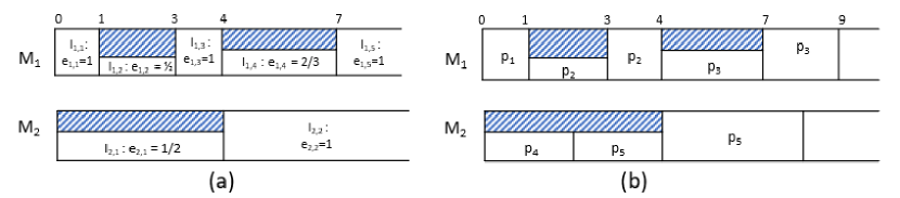
Figure 1: An example of multitasking scheduling on 2 machines with shared processing, 3 routine jobs are shown as shaded intervals. (a) The intervals and the sharing ratios; (b) A schedule of the 5 primary jobs with the processing times of 1, 2, 4, 1, 5.

As we addressed earlier, routine job management, independent from the primary job scheduling, has predetermined the time interval during which a routine job is processed, the machine on which the routine job is processed, and the machine capacity that is assigned to a routine job. So we are only concerned with the schedule of the primary jobs when some fraction of the machine capacity has been assigned to the routine jobs during some time intervals on some machines. In this sense, we can view each machine consisting of intervals with full capacity alternating with those intervals with a fraction of machine capacity, and we use “sharing ratio” to refer to the fraction of the capacity available to the primary jobs, which is in the range of $(0,1]$. Apparently, each machine $M_{i}$ $(1\leq i\leq m)$ has $O(k_{i})$ intervals in total. Without loss of generality, we assume that these intervals are given in sorted order, denoted as $I_{i,1}=(0,t_{i,1}]$, $I_{i,2}=(t_{i,1},t_{i,2}]$, $\ldots$, and their corresponding sharing ratios are $e_{i,1}$, $e_{i,2}$, $\ldots$, all of which are in the range of $(0,1]$, see Figure 1 (a) for an illustration of machine intervals and Figure 1 (b) for an illustration of one schedule of primary jobs in these intervals.

In this paper, we focus on two objectives: minimizing the makespan and minimizing the total completion time of the primary jobs. For any schedule $S$, let $C_{j}(S)$ be the completion time of the primary job $j$ in $S$. If the context is clear, we use $C_{j}$ for short. The makespan of the schedule $S$ is $C_{max}(S)=\max_{1\leq j\leq n}\{C_{j}\}$ and the total completion time of the schedule $S$ is $\sum C_{j}(S)=\sum_{1\leq j\leq n}\{C_{j}\}$. Using the three-field $\alpha\mid\beta\mid\gamma$ notation introduced by Graham et al. [8], our problems are denoted as $P_{m},e_{i,k}\mid\mid C_{max}$ and $P_{m},e_{i,k}\mid\mid\sum C_{j}$ if the sharing ratios are arbitrary; if all the sharing ratios have a constant lower bound $e_{0}$ ($0<e_{0}\leq 1$), our problems are denoted as $P_{m},e_{i,k}\geq e_{0}\mid\mid C_{max}$ and $P_{m},e_{i,k}\geq e_{0}\mid\mid\sum C_{j}$; and if the sharing ratio is at least $e_{0}$ for the intervals on the first $m_{1}$ ($1\leq m_{1}\leq m-1$) machines but arbitrary for other $(m-m_{1})$ machines, our problems are denoted as $P_{m},e_{i\leq m_{1},k}\geq e_{0}\mid\mid C_{max}$ and $P_{m},e_{i\leq m_{1},k}\geq e_{0}\mid\mid\sum C_{j}$.

1.2 Literature Review

The shared processing multitasking model studied in this paper was first proposed by Hall et. al. in [10]. They studied this model in the single machine environment and assumed that the sharing ratio is a constant $e$ for all the shared intervals. For this model, it is easy to see that the makespan is the same for all schedules that have no unnecessary idle time. The authors in [10] showed that the total completion time can be minimized by scheduling the jobs in non-decreasing order of the processing time, but it is unary NP-Hard for the objective function of total weighted completion time. When the primary jobs have different due dates, the authors gave polynomial time algorithms for maximum lateness and the number of late jobs.

For the related work, Baker and Nuttle [2] studied the problems of sequencing $n$ jobs for processing by a single resource to minimize a function of job completion times subject to the constraint that the availability of the resource varies over time. The motivation for this machine environment comes from the situation in which processing requirements are stated in terms of labor-hours and labor availability varies over time. The example can be found in the applications of rotating Saturday shifts, where the company only maintains a fraction, for example 33%, of the workforce every Saturday. The authors showed that a number of well-known results for classical single-machine problems can be applied with little or no modification to the corresponding variable-resource problems. Hirayama and Kijima [13] studied this problem when the machine capacity varies stochastically over time. Adiri and Yehudai [1] studied the problem on single and parallel machines such that if a job is being processed, the service rate of a machine remains constant and the service rate can be changed only when the job is completed.

So far there are no results about the problems studied in this paper. Note that if $e_{i,k}=1$ for all time intervals, that is, there are no routine jobs, our problems become the classical parallel machine scheduling problems $P_{m}\mid\mid C_{max}$ and $P_{m}\mid\mid\sum C_{j}$. The problem $P_{m}\mid\mid\sum C_{j}$ can be solved optimally using SPT (Shortest Processing Time First) rule, which schedules the next shortest job to the earliest available machine. The problem $P_{m}\mid\mid C_{max}$ is a NP-Hard problem and some approximation algorithms have been designed for it. Graham showed in [6] that LS (List Scheduling) rule generates a schedule with an approximation ratio of $2-\tfrac{1}{m}$. The LS rule schedules the jobs one by one in the given ordered list. Each job is assigned in turn to a machine which is available at the earliest time. If the given list is in non-increasing order of the processing time of the jobs, the list schedule rule is called LPT ( the Longest Processing Time First) rule. In [1], Graham showed that LPT rule generates a schedule whose approximation ratio is $(\tfrac{4}{3}-\tfrac{1}{3m})$. Hochbaum and Shmoys [14] designed a PTAS for this problem. When the number of machines $m$ is fixed, Horowitz and Sahni [15] developed an FPTAS.

On the other hand, if $e_{i,k}\in\{0,1\}$ for all time intervals, i.e. at any time the machine is either processing a primary job or a routine job but not both, then our problems reduce to the problems of parallel machine scheduling with availability constraint where jobs can be resumed on after being interrupted: $P_{m}|r-a|C_{max}$ and $P_{m}|r-a|\sum C_{j}$. The problem $P_{m}|r-a|C_{max}$ is NP-hard and approximation algorithms are developed in [16] and [17]. The problem $P_{m}|r-a|\sum C_{j}$ is NP-hard when $m=2$ and one machine becomes unavailable after some finite time [18]. In the same paper Lee and Liman show that the SPT rule with some modifications leads to a tight relative error of $\tfrac{1}{2}$ for $P_{2},NC_{zz}\mid\mid\sum C_{j}$ where one machine is continuously available and the other machine becomes unavailable after some finite time.

1.3 New Contribution

In this paper, we generalize the shared processing multitasking model proposed by Hall et. al. in [10] to parallel machine environment and allow the processing capacity to be different for different routine jobs.

For the objective of makespan, we show that there is no approximation algorithm for the problem $P_{m},e_{i,k}\mid\mid C_{max}$ (that is, the sharing ratios are arbitrary for all shared intervals) unless $P=NP$. Then for a fixed $e_{0}$, $0<e_{0}<1$, we analyze the performance of the LS rule, LS-ECT (List Scheduling - Earliest Completion Time) rule, LPT and LPT-ECT (Largest Processing Time - Earliest Completion Time) rule for the problems $P_{m},e_{i,k}\geq e_{0}\mid\mid C_{max}$ and $P_{m},e_{i\leq m_{1},k}\geq e_{0}\mid\mid C_{max}$. We then develop an approximation scheme for the problem $P_{m},e_{i\leq m_{1},k}\geq e_{0}\mid\mid C_{max}$ whose running times is linear time when the number of machines is a constant.

For the objective of total completion time, we show that there is no approximation algorithm for the general problem $P_{m},e_{i,k}\mid\mid\sum C_{j}$ (that is, the sharing ratios are arbitrary for all intervals) unless $P=NP$. Then for $P_{m},e_{i\leq m_{1},k}\geq e_{0}\mid\mid\sum C_{j}$, that is, the sharing ratios are at least $e_{0}$ for the intervals on the first $m_{1}$ ($1\leq m_{1}\leq m-1$) machines but arbitrary for other $(m-m_{1})$ machines, we analyze the performance of the SPT rule and SPT-ECT (Shortest Processing Time - Earliest Completion Time) rule, and show that SPT-ECT is a $\left\lceil\tfrac{m}{m_{1}}\right\rceil\tfrac{1}{e_{0}}$-approximation algorithm while SPT can perform arbitrarily bad. We then develop an approximation scheme for the problem $P_{m},e_{i\leq m-1,k}\geq e_{0}\mid\mid\sum C_{j}$.

The paper is organized as follows. In Section 2, we study the problems with the objective of makespan minimization. In Section 3, we study the problems with the objective of the total completion time minimization. At last in Section 4 we draw the concluding remarks.

2 Makespan Minimization

2.1 Hardness for Approximation

In this section, we show that if the processor sharing intervals and the sharing ratios in these intervals are arbitrary, then no approximation algorithm exists.

Theorem 1.

Let $\mathbb{N}$ be the set of natural numbers. Let $f(n):\mathbb{N}\rightarrow\mathbb{N}$ be an arbitrary function such that $f(n)>1$. There is no polynomial time $f(n)$-approximation algorithm for $P_{m},e_{i,k}\mid\mid C_{\max}$ even if $m=2$ unless $P=NP$.

Proof.

We prove the inapproximability by reducing from the partition problem.

Partition Problem: Given a set of positive integers $\{a_{1},\cdots,a_{n}\}$ where $A=\sum_{i=1}^{n}a_{i}$ is even, find if the set can be partitioned into two sets with equal sum $\frac{1}{2}A$.

Given an instance of partition problem, we can reduce it to an instance of our scheduling problem as follows: There are two machines, $n$ primary jobs, for each job $j$, $p_{j}=a_{j}$. There are two routine jobs, one for each machine, both of which are during the interval $[\tfrac{A}{2},\tfrac{A}{2}+f(n)\cdot A]$ with the sharing ratio of $e=\tfrac{1}{f(n)\cdot A}$.

We will show that if there is an $f(n)$-approximation algorithm for the scheduling problem, then the algorithm returns a schedule with makespan at most $\tfrac{A}{2}\cdot f(n)$ for the constructed scheduling problem instance if and only if there is a partition to the given partition instance.

Apparently, the makespan of any schedule of the primary jobs is at least $\tfrac{A}{2}$. Also if a job can’t finish at $\tfrac{A}{2}$, it will then takes at least $f(n)A$ additional time due to the processing sharing. Thus the makespan of any schedule is either exactly $\tfrac{A}{2}$, or at least $\tfrac{A}{2}+f(n)A=\tfrac{A}{2}(1+2f(n))$. Therefore, if the approximation algorithm returns a schedule whose makespan is at most $\tfrac{A}{2}\cdot f(n)$, then the makespan of the schedule must be exactly $\tfrac{A}{2}$. This implies that there is a partition to the integers.

On the other hand, if there is a partition, i.e., the numbers can be partitioned into two sets, each having a sum exactly $\tfrac{A}{2}$, then the optimal schedule will schedule the corresponding jobs in each set to a machine and its makespan is exactly $\tfrac{A}{2}$. Then the $f(n)$-approximation algorithm must return a schedule whose makespan is at most $\tfrac{A}{2}\cdot f(n)$.

The above analysis shows that the integer partition problem has a solution if and only if the algorithm returns a schedule with completion time at most $\tfrac{A}{2}f(n)$ for the corresponding scheduling instance. Since the partition problem is NP-hard, unless P=NP, there is no such approximation algorithm. ∎

Given the inapproximability result from Theorem 1, from now on, we will focus on the problems $P_{m},e_{i,k}\geq e_{0}\mid\mid C_{max}$ and $P_{m},e_{i\leq m-1,k}\geq e_{0}\mid\mid C_{max}$.

2.2 Approximation Algorithms

2.2.1 Preliminary

First, we consider the problem $P_{m},e_{i,k}\geq e_{0}\mid\mid C_{max}$ where the sharing ratio is bounded below by a constant $e_{0}$ for all intervals, i.e. $e_{i,k}\geq e_{0}$ for all machines $M_{i}$, $1\leq i\leq m$.

We have the following observation: Let $I$ be an instance for $P_{m},e_{i,k}\geq e_{0}\mid\mid C_{\max}$, and $I^{\prime}$ be the corresponding instance for $P_{m}\mid\mid C_{\max}$. Let $S^{\prime}$ be a schedule for $I^{\prime}$ and $S$ be the corresponding schedule for $I$. Then the completion time of a job $j$ in $S$ is at most $\tfrac{1}{e_{0}}$ times that in $S^{\prime}$. It is easy to see that the optimal makespan for $I$ must be greater than or equal to that of $I^{\prime}$, thus we can get the following observation.

Observation 2.

An $\alpha$-approximation algorithm for $P_{m}\mid\mid C_{\max}$ is an $\tfrac{\alpha}{e_{0}}$-approximation algorithm for $P_{m},e_{i,k}\geq e_{0}\mid\mid C_{\max}$.

Observation 2 and the existing literature [7, 14, 15] imply the following results for $P_{m},e_{i,k}\geq e_{0}\mid\mid C_{\max}$:

1. LS rule is a $(2-\tfrac{1}{m})\tfrac{1}{e_{0}}$-approximation.

2. LPT rule is a $(\tfrac{4}{3}-\tfrac{1}{3m})\tfrac{1}{e_{0}}$-approximation.

3. There is a $\tfrac{1+\epsilon}{e_{0}}$ approximation whose running time is $O(n^{2k}\left\lceil\log_{2}\tfrac{1}{\epsilon}\right\rceil)$, where $k=\left\lceil\log_{1+\epsilon}\tfrac{1}{\epsilon}\right\rceil$.

4. There is a $\tfrac{1+\epsilon}{e_{0}}$ approximation whose running time is $O(n(n^{2}/\epsilon)^{m-1})$.

It turns out the above bound for LS rule is quite loose. In the following, we will give a tighter bound.

2.2.2 List Scheduling (LS) rule

For an instance of $P_{m},e_{i,k}\geq e_{0}\mid\mid C_{\max}$, let $C_{max}(LS)$ and $C_{max}^{*}$ be the makespan of an arbitrary list schedule and the optimal schedule, respectively. Then we have the following theorem.

Theorem 3.

For $P_{m},e_{i,k}\geq e_{0}\mid\mid C_{\max}$, $\tfrac{C_{\max}(LS)}{C_{max}^{*}}\leq(1+\tfrac{1}{e_{0}})$ .

Proof.

Without loss of generality, we assume $C_{\max}(LS)=C_{j}$ for some job $j$. Assume that job $j$ starts at time $t$ in the list schedule. This means there is no idle time before $t$ and we must have $C_{max}^{*}>t$, and $C_{\max}(LS)=C_{j}\leq t+\tfrac{p_{j}}{e_{0}}\leq C_{max}^{*}+C_{max}^{*}\cdot\tfrac{1}{e_{0}}=C_{max}^{*}(1+\tfrac{1}{e_{0}})$. ∎

Complexity of List Scheduling Given a list, the list scheduling can be implemented as follows. For a partial schedule, we maintain the completion time of the last job $f_{i}$, $1\leq i\leq m$, on all machines using a min-heap. The next job $j$ in the list will be assigned to the machine with minimum $f_{i}$, which can be found and updated in $O(k+\log m)$ time, where $k$ is the number of intervals during which the job $j$ is scheduled. The total running time to assign all $n$ jobs will be $O(n\log m+\tilde{n})$. If we use LPT rule, then we need additional time to sort the jobs and the total time would be $O(n\log n+n\log m+\tilde{n})=O(n\log n+\tilde{n})$.

2.2.3 Modified List Scheduling - LS-ECT and LPT-ECT

If we relax the constraint on sharing ratios from $P_{m},e_{i,k}\geq e_{0}\mid\mid C_{\max}$, so that only the intervals on the first $m_{1}$ machines have bounded sharing ratios, i.e., $P_{m},e_{i\leq m_{1},k}\geq e_{0}\mid\mid C_{max}$, LS rule could perform very badly. Consider the example of 2 machines, the first machine has a bounded sharing interval $(0,\infty)$ with sharing ratio $e_{0}$, the second machine has a sharing interval $(0,\infty)$ with sharing ratio $x<<e_{0}$, and we have two jobs of length 1. The LS schedule will schedule one job on each machine and the makespan will be $1/x$, but the optimal schedule will schedule both jobs on the first machine and has a makespan of $\tfrac{2}{e_{0}}$. The approximation ratio of LS is $\tfrac{e_{0}}{2x}$, which will be arbitrarily large as $x$ gets close to 0.

To have a better approximation for the more general problem $P_{m},e_{i\leq m_{1},k}\geq e_{0}\mid\mid C_{max}$, we want to consider a modified list scheduling for our model: when we schedule the next job $j$ in the list, instead of scheduling it to the machine so that it can start as early as possible, schedule it to the machine so that it can complete the earliest. We will call this heuristic LS-ECT, and we call it LPT-ECT if the list is in LPT order. We use $C_{max}$(LS-ECT) and $C_{max}$(LPT-ECT) to denote the makespan of the schedule produced by LS-ECT and LPT-ECT respectively.

Before we do further analysis, we give some simple facts and a claim that we will use frequently later. Let $S$ be any schedule without any unnecessary idle time. Let $f_{i}$, $1\leq i\leq m$, denote the completion time of the last job on machine $M_{i}$ in $S$.

1. Fact 1: There exists at least one $f_{i}$ such that $f_{i}\leq C_{max}^{*}$.

2. Fact 2: Let $S$ be an LS-ECT schedule. If the last job $j$ on machine $M_{i_{1}}$ starts at a time later than $f_{i_{2}}$, then rescheduling job $j$ to $M_{i_{2}}$ does not decrease its completion time.

Claim 4.

Let $S$ be an LS-ECT schedule and $X$ be the number of jobs that complete after $C_{max}^{*}$ on the first $m_{1}$ machines, if $f_{i}>C_{max}^{*}$ for all $1\leq i\leq m_{1}$, then $X\leq m-1$.

Proof.

Suppose not, then $X\geq m$. Among these $X$ jobs, we remove $(m-m_{1})$ jobs so that the last job on the first $m_{1}$ machines are still completed after $C_{max}^{*}$, and reschedule each of the $(m-m_{1})$ jobs to one of the last $m-m_{1}$ machines. By Fact 2, the completion times of all these jobs do not decrease, so their completion times are all still larger than $C_{max}^{*}$, and thus all machines are busy after $C_{max}^{*}$, which contradicts Fact 1. This concludes the proof of the claim. ∎

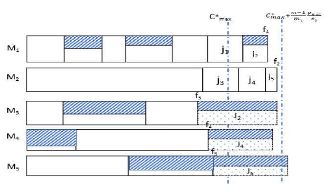
Figure 2: An LS-ECT schedule for $P_{m},e_{i\leq m_{1},k}\geq e_{0}\mid\mid C_{max}$ where $m=5$, $m_{1}=2$, and $f_{i}\geq C_{max}^{*}$ for all $i\leq m_{1}$. It is impossible that 5 or more jobs finish later after $C_{max}^{*}$ on the first $m_{1}=2$ machines.

Figure 2 illustrates the proof of Claim 4 where $m=5$, $m_{1}=2$, and $X=5$. Among the 5 jobs that finish after $C_{max}^{*}$ on the first 2 machines, if we reschedule the jobs $2,4,5$ to the last three machines, respectively, all the machines are busy after $C_{max}^{*}$, and this contradicts Fact 1.

In the following, we consider the performance of LS-ECT for the problem $P_{m},e_{i\leq m_{1},k}\geq e_{0}\mid\mid C_{max}$.

Theorem 5.

For $P_{m},e_{i\leq m_{1},k}\geq e_{0}\mid\mid C_{max}$,

$$\frac{C_{max}(\text{LS-ECT})}{C_{max}^{*}}\leq\left(1+\tfrac{1}{e_{0}}\cdot\left(\left\lfloor\tfrac{m-1}{m_{1}}\right\rfloor+1\right)\right).$$

Proof.

Let $I$ be the smallest instance for which LS-ECT has the worst performance. Assume the jobs are ordered 1, 2, …, n, then we must have $C_{max}(\text{LS-ECT})=C_{n}$. Suppose not, then we can remove job $n$ to get a new instance. For the new instance, the performance ratio of LS-ECT will be the same or worse because the makespan of LS-ECT schedule will be the same, but the optimal makespan may be smaller, which contradicts to the fact that $I$ is the smallest instance for which LS-ECT has the worst performance.

Let $S$ be the schedule obtained for $I$ using LS-ECT where $f_{i}$, $1\leq i\leq m$, is the completion time of the last job on machine $M_{i}$ in the LS-ECT schedule. By Fact 1, there exists at least one $f_{i}$ such that $f_{i}\leq C_{max}^{*}$.

If $f_{i}\leq C_{max}^{*}$ for some $i\leq m_{1}$, then if we reschedule job $n$ to $M_{i}$, its new completion time will be at most $f_{i}+p_{n}/e_{0}\leq(1+\tfrac{1}{e_{0}})C_{max}^{*}$. By Fact 2, this will not be better than its original completion time. Thus in this case we have $C_{max}(\text{LS-ECT})=C_{n}\leq(1+\tfrac{1}{e_{0}})C_{max}^{*}$. See Figure 3 for an illustration.

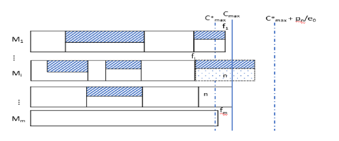
Figure 3: An LS-ECT schedule for $P_{m},e_{i\leq m_{1},k}\geq e_{0}\mid\mid C_{max}$ where $f_{i}\leq C_{max}^{*}$, $i\leq m_{1}$. If job $n$ were rescheduled to $M_{i}$, it would finish no earlier than its current completion time.

Otherwise, we have $f_{i}>C_{max}^{*}$ for all $1\leq i\leq m_{1}$, and for some machine $M_{i^{\prime}}$, $i^{\prime}>m_{1}$, $f_{i^{\prime}}<C_{max}^{*}$. By Claim 4, we know there are at most $X\leq m-1$ jobs complete after $C_{max}^{*}$ on the first $m_{1}$ machines. By pigeon hole principle, among the first $m_{1}$ machines, there exists a machine on which there are at most $\left\lfloor X/m_{1}\right\rfloor\leq\left\lfloor(m-1)/m_{1}\right\rfloor$ jobs finishing after $C_{max}^{*}$. Without loss of generality, suppose $n$ is not scheduled on this machine, then moving job $n$ to this machine will not decrease its completion time. Let $p_{max}=\max_{1\leq j\leq n}p_{j}$, then we have

$$C_{max}=C_{n}\leq C_{max}^{*}+\left\lfloor\tfrac{m-1}{m_{1}}\right\rfloor\tfrac{p_{max}}{e_{0}}+\tfrac{p_{n}}{e_{0}}\leq\left(1+\left(\left\lfloor\tfrac{m-1}{m_{1}}\right\rfloor+1\right)\cdot\tfrac{1}{e_{0}}\right)C_{max}^{*}.$$

∎

Theorem 5 implies that if $m_{1}=m$, the ratio of LS-ECT is $(1+\tfrac{1}{e_{0}})$ which agrees with the ratio of LS rule from Theorem 3. If $m_{1}=m-1$, the approximation from Theorem 5 becomes $(1+\tfrac{2}{e_{0}})$, which is worse than the case $m_{1}=m$. In the following we show that in this case, the approximation ratio is actually still bounded by $(1+\tfrac{1}{e_{0}})$.

Theorem 6.

For $P_{m},e_{i\leq m-1,k}\geq e_{0}\mid\mid C_{max}$,

$$\frac{C_{max}\text{(LS-ECT)}}{C_{max}^{*}}\leq 1+\tfrac{1}{e_{0}}.$$

Proof.

Let $I$ be the smallest instance for which LS-ECT has the worst performance. Assume the jobs are ordered 1, 2, …, n, then we must have $C_{max}(\text{LS-ECT})=C_{n}$.

Let $S$ be the schedule obtained for $I$ using LS-ECT where $f_{i}$, $1\leq i\leq m$, is the completion time of the last job on machine $M_{i}$ in $S$. By Fact 1, there exists at least one $f_{i}$ such that $f_{i}\leq C_{max}^{*}$.

If $i\leq m-1$, then as in the proof of Theorem 5, we have $C_{max}(\text{LS-ECT})=C_{n}\leq(1+\tfrac{1}{e_{0}})C_{max}^{*}$.

Otherwise, there is no $i$ such that $i\leq m-1$ and $f_{i}\leq C_{max}^{*}$. This implies (1) on each of the first $(m-1)$ machines, at least one job finishes after $C_{max}^{*}$, (2) $f_{m}<C_{max}^{*}$, and (3) job $n$ must be scheduled on one of the first $(m-1)$ machines. By Claim 4, there are at most $(m-1)$ jobs that complete after $C_{max}^{*}$ on the first $m-1$ machines. Combining with (1), there is exactly one job that completes after $C_{max}^{*}$ for each $M_{i}$, $i\leq m-1$. Therefore, $n$ must be the only job that finishes after $C_{max}^{*}$ on the machine it is scheduled; and it starts at or before $C_{max}^{*}$. So we have $C_{max}(\text{LS-ECT})=C_{n}\leq C_{max}^{*}+p_{n}/e_{0}\leq(1+\tfrac{1}{e_{0}})C_{max}^{*}$. ∎

A natural question follows from Theorem 6 is if the performance of LS-ECT is still $(1+\tfrac{1}{e_{0}})$ when $m_{1}=m-2$. We show by an example that this is unfortunately not the case. We have $m=3$ and $m_{1}=1$. The first machine has a sharing ratio of ${e_{0}}$ during interval $[x+2,\infty)$, the other 2 machines have sharing ratio $\tfrac{e_{0}}{3x}$ during interval $[x,\infty)$, and all other intervals have sharing ratio 1; there are 5 jobs whose processing times are x, 1, 1, x, x. If we use this list for LS-ECT, the first machine has three large jobs, and the other two machines each has one small job, and the makespan is $(x+2+\tfrac{2x-2}{e_{0}})$; however in the optimal schedule, one large job and the two small jobs are scheduled on the first machine, and the other two large jobs are scheduled on the second and third machines, respectively. The makespan of the optimal schedule is $(x+2)$. The performance ratio of LS-ECT approaches to $(1+\tfrac{2}{e_{0}})$ as $x$ increases.

Note that if $e_{0}=1$, the approximation ratio obtained from Theorem 6 becomes 2 which is very close to the ratio $(2-1/m)$ of LS rule for classical model where all machines have full capacity.

We also want to point out that for LPT-ECT, we can get slightly better ratios than those for LS-ECT in Theorem 5 and 6. Based on the fact $C_{max}^{*}\geq\tfrac{\sum p_{j}}{m}$, and the fact for LPT that $p_{n}\leq\tfrac{\sum p_{j}}{n}$, we have $p_{n}/e_{0}\leq\tfrac{m}{ne_{0}}C_{max}^{*}$. Then we can get the following result for LPT-ECT.

Corollary 7.

For $P_{m},e_{i\leq m_{1},k}\geq e_{0}\mid\mid C_{max}$,

$$\frac{C_{max}(\text{LPT-ECT})}{C_{max}^{*}}\leq\left(1+\frac{1}{e_{0}}\cdot\left(\left\lfloor\frac{m-1}{m_{1}}\right\rfloor+\frac{m}{n}\right)\right),$$

and for $P_{m},e_{i\leq m-1,k}\geq e_{0}\mid\mid C_{max}$,

$$\frac{C_{max}(\text{LPT-ECT})}{C_{max}^{*}}\leq 1+\frac{m}{ne_{0}}.$$

Time Complexity

Compared with LS rule, LS-ECT takes more time for each job because we need to compare its completion times on all machines and schedule it to the machine so that it completes at the earliest time.

To implement LS-ECT, considering a partial schedule where jobs $1$, $2$, $\ldots$, $j-1$ have been scheduled, we maintain a pair $(P_{i},f_{i})$ for each machine $M_{i}(1\leq i\leq m)$, where $P_{i}$ is the total processing time of the jobs that have been assigned to $M_{i}$, and $f_{i}$ is the completion time of the last job on $M_{i}$. Moreover, for each interval on machine $M_{i}$, $I_{i,1}=(0,t_{i,1}]$, $I_{i,2}=(t_{i,1},t_{i,2}]$, $\ldots$, we maintain a quadruple $(t_{i,k-1},t_{i,k},e_{i,k},A_{i}(t_{i,k}))$ where $e_{i,k}$ is the sharing ratio of the interval $(t_{i,k-1},t_{i,k}])$ and $A_{i}(t_{i,k})$ is the total amount of the jobs that can be scheduled before $t_{i,k}$. For convenience of scheduling, we pre-calculate $A_{i}(t_{i,k})$ for every $t_{i,k}$ on machine $M_{i}$. Note that $A_{i}(t_{i,k})=A_{i}(t_{i,k-1})+e_{i,k}(t_{i,k}-t_{i,k-1})$. Assuming the intervals are given in sorted order, the calculation can be done in $O(k_{i})$ time for machine $M_{i}$ where $k_{i}$ is the number of shared intervals on $M_{i}$, and in $O(\tilde{n})$ for all $m$ machines.

To assign a job $j$ to this partial schedule, for each machine $M_{i}$, we can use binary search on the continuous intervals $I_{i,1}$, $I_{i,2}$, $\ldots$, to find the interval $(t_{i,k-1},t_{i,k}]$ such that $A_{i}(t_{i,k-1})<P_{i}+p_{j}\leq A_{i}(t_{i,k}$). Then job $j$’s completion time on machine $M_{i}$ can be calculated as $t=t_{i,k-1}+\tfrac{P_{i}+p_{j}-A_{i}(t_{i,k-1})}{e_{i,k}}$. After all machines are considered, we assign job $j$ to the machine so it completes the earliest. In total, it takes $O((\sum_{i=1}^{m}\log k_{i})+m)$ time to assign a job to the machine so it completes the earliest. So the overall time for scheduling $n$ jobs using LS-ECT is $O(\tilde{n}+n(m+\sum_{i=1}^{m}\log k_{i}))$, and the total time for LPT-ECT is $O(n\log n+\tilde{n}+n(m+\sum_{i=1}^{m}\log k_{i}))$.

2.2.4 Comparison of List Scheduling and Modified List Scheduling

While LS gives the approximation ratio of $(1+\tfrac{1}{e_{0}})$ for problem $P_{m},e_{i,k}\geq e_{0}\mid\mid C_{max}$, it can perform badly for problem $P_{m},e_{i\leq m_{1},k}\geq e_{0}\mid\mid C_{max}$. In comparison, the approximation ratio of LS-ECT for $P_{m},e_{i\leq m_{1},k}\geq e_{0}\mid\mid C_{max}$ is $\left(1+\tfrac{1}{e_{0}}\cdot\left(\left\lfloor\tfrac{m-1}{m_{1}}\right\rfloor+1\right)\right)$. And when $m_{1}=m-1$, LS-ECT gives the approximation ratio of $(1+\tfrac{1}{e_{0}})$. Similar conclusions hold for LPT rule and LPT-ECT rule.

Now we consider the performance of LPT and LPT-ECT when the number of jobs is small. When $n\leq 2m$, LPT is optimal for $P_{m}\mid\mid C_{\max}$, however, this does not hold any more for $P_{m},e_{i,k}\geq e_{0}\mid\mid C_{max}$ even if $n=2$. Consider the example of two machines and two jobs of length 1. Suppose the first machine doesn’t have processor sharing, while the second machine has a sharing interval $[0,\infty)$ with $e_{2,1}=e_{0}<\tfrac{1}{2}$. The optimal schedule has both jobs on the first machine with the makespan of 2, but LPT rule schedules one job on each machine and thus has an approximation ratio of $\tfrac{1}{2e_{0}}$. Although LPT-ECT can find the optimal schedule when there are only two jobs, it is not optimal anymore when the number of jobs $n\geq 3$. Consider three jobs of length 3, 2, 2 and two machines. There is a single sharing interval $I_{2,1}=[0,\infty)$, and $e_{2,1}=3/4$. The LPT-ECT will schedule one shorter job on $M_{2}$, and the other two jobs on $M_{1}$ with the makespan $5$ while the optimal schedule schedules the longest job on $M_{2}$ and the 2 shorter jobs on $M_{1}$, and the makespan is 4.

2.3 Approximation Scheme

In this section, we develop an approximation scheme for $P_{m},e_{i\leq m_{1},k}\geq e_{0}\mid\mid C_{max}$. The idea is to partition the jobs into two groups, one for large jobs and the other for small jobs. Then we schedule the large jobs using enumeration; and schedule the small jobs using LS-ECT. Let $d$ be the number of large jobs which determines the error ratio of the output schedule and will be specified later. Our algorithm is formally presented as follows.

Algorithm 1

Input:

• Parameters $m$, $n$, $m_{1}$, and $e_{0}$

• The intervals $(0,t_{i,1}]$, $(t_{i,1},t_{i,2}]$, $\ldots$ on machine $M_{i}$, $1\leq i\leq m$, and their sharing ratios $e_{i,1}$, $e_{i,2}$, $\ldots$, respectively

• The jobs’ processing time $p_{j}$, $1\leq j\leq n$

• Integer parameter $d$ that determines the accuracy of approximation

Output: a schedule of the $n$ jobs

Steps:

1. Find the $d$ largest jobs

2. For each possible assignment of the large jobs

3. Schedule the remaining jobs using LS-ECT

4. Return the schedule $S$ obtained from previous step that has the minimum makespan

For ease of analysis, we first analyze the performance of Algorithm 1 for $m_{1}=m$, i.e. $P_{m},e_{i,k}\geq e_{0}\mid\mid C_{max}$, then the general case $m_{1}\leq m$, i.e., $P_{m},e_{i\leq m_{1},k}\geq e_{0}\mid\mid C_{max}$. Let $S^{*}$ be an optimal schedule and $C_{\max}^{*}$ be the makespan of $S^{*}$.

Lemma 8.

For an instance of $P_{m},e_{i,k}\geq e_{0}\mid\mid C_{max}$, Algorithm 1 returns a schedule with the makespan at most $(1+\tfrac{m}{d\cdot e_{0}})\cdot C_{\max}^{*}$.

Proof.

Let $p_{d}$ be the processing time of the $d$-th largest job. Then we must have $C^{*}_{\max}\geq\tfrac{d\cdot p_{d}}{m}$. Thus, $p_{d}\leq\tfrac{m}{d}C^{*}_{\max}$.

Let $S^{\prime}$ be the schedule obtained from step 2 of Algorithm 1 that has the same large job assignment as $S^{*}$. Let $j$ be the job such that $C_{j}(S^{\prime})=C_{max}(S^{\prime})$. Without loss of generality, we can assume $C_{max}(S^{\prime})>C_{\max}^{*}$. Then $j$ must be a small job. By Fact 1, there is at least one machine such that the last job on this machine finishes at or before $C_{\max}^{*}$ in any schedule. Let $M_{i}$ be such a machine in $S^{\prime}$. Then job $j$ must be scheduled on a machine other than $M_{i}$ in $S^{\prime}$. By Fact 2, if job $j$ is rescheduled to $M_{i}$ in $S^{\prime}$, then its new completion time, at most $C^{*}_{\max}+\frac{p_{j}}{e_{0}}$, would not be less than its original completion time $C_{\max}(S^{\prime})$ (see Figure 4). Therefore, we have

$$C_{\max}(S^{\prime}) \leq C^{*}_{\max}+\frac{p_{j}}{e_{0}}$$

$$\leq C^{*}_{\max}+\frac{1}{e_{0}}p_{d}$$

$$\leq C^{*}_{\max}+\frac{1}{e_{0}}\cdot\tfrac{m}{d}C^{*}_{\max}$$

$$\leq \left(1+\frac{m}{d\cdot e_{0}}\right)\cdot C^{*}_{\max}.$$

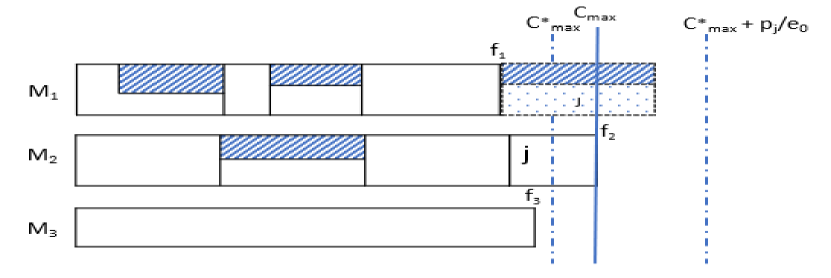
Figure 4: Illustration of schedule $S^{\prime}$ obtained from Algorithm 1: $C_{max}(S^{\prime})=C_{j}$, if job $j$ were scheduled on $M_{1}$, it would finish no earlier than its current completion time.

Since Algorithm 1 returns a schedule $S$ with minimum makespan, the above bound is also an upper bound of $C_{\max}(S)$. ∎

Lemma 9.

Algorithms 1 can be implemented in $O(\tilde{n}+n+(m^{d}(n-d)(m+\sum_{i=1}^{m}\log k_{i})))$ time.

Proof.

In step 1, we first find the $d$-th largest job using linear selection algorithm, and then extract the $d$ largest jobs in $O(n)$ time. In step 2, there are at most $m^{d}$ ways to assign these large jobs to $m$ machines. For each large job assignment, the algorithm schedules the remaining small jobs using LS-ECT rule. As we described in the Section 2.2.3 for the time complexity analysis, with $A_{i}(t_{i,k})$ pre-calculated in $O(\tilde{n})$ time, it takes $O((\sum_{i=1}^{m}\log k_{i})+m)$ time to assign a job to the machine so it completes the earliest. So for each large job assignment, the overall time for scheduling $(n-d)$ small jobs using LS-ECT in step 2 is $O((n-d)(m+\sum_{i=1}^{m}\log k_{i}))$. Adding all the time, we get the total running time of Algorithm 1 $O(\tilde{n}+n+m^{d}(n-d)(m+\sum_{i=1}^{m}\log k_{i}))$ ∎

Given an instance of $P_{m},e_{i,k}\geq e_{0}\mid\mid C_{max}$, and a real number $\epsilon\in(0,1)$, if we select $d=\left\lceil\tfrac{m}{\epsilon e_{0}}\right\rceil$ and apply algorithm 1, then by Lemma 8, we get a schedule $S$ whose makespan is at most $(1+\epsilon)C^{*}_{\max}$. Combining Lemma 8 and Lemma 9, we get the following theorem.

Theorem 10.

For any given instance of $P_{m},e_{i,k}\geq e_{0}\mid\mid C_{max}$ and an error parameter $\epsilon$, $0<\epsilon<1$, Algorithm 1 can return a schedule with makespan at most $(1+\epsilon)C_{max}^{*}$ in $O(\tilde{n}+n+m^{{m}/({\epsilon\cdot e_{0}})}(n-\tfrac{m}{\epsilon\cdot e_{0}})(m+\sum_{i=1}^{m}\log k_{i}))$ time.

Next we analyze the performance of Algorithm 1 for the more general problem $P_{m},e_{i\leq m_{1},k}\geq e_{0}\mid\mid C_{max}$. We will show that by choosing $d$ appropriately, we can still get a $(1+\epsilon)$ approximation.

Theorem 11.

For any given instance of $P_{m},e_{i\leq m_{1},k}\geq e_{0}\mid\mid C_{max}$ and a parameter $d$, Algorithm 1 returns a schedule with makespan at most $(1+\frac{m(m+m_{1}-1)}{d\cdot e_{0}\cdot m_{1}})C_{max}^{*}$ in $O(\tilde{n}+n+m^{d}(n-d)(m+\sum_{i=1}^{m}\log k_{i}))$ time. In particular, if $d=\left\lceil\tfrac{m(m+m_{1}-1)}{\epsilon\cdot e_{0}\cdot m_{1}}\right\rceil$, it is a $(1+\epsilon)$-approximation.

Proof.

As in the proof of Lemma 8, we consider the schedule $S^{\prime}$ from step 2 of Algorithm 1 that has the same assignment of large jobs as the optimal schedule $S^{*}$. Let $j$ be the job such that $C_{j}(S^{\prime})=C_{\max}(S^{\prime})$. Without loss of generality, we assume $C_{\max}(S^{\prime})>C_{\max}(S^{*})$, then $j$ must be a small job. Let $p_{d}$ be the processing time of the $d$-th largest job. Then we must have $C^{*}_{\max}\geq\tfrac{d\cdot p_{d}}{m}$, that is, $p_{d}\leq\tfrac{m}{d}C^{*}_{\max}$. By Fact 1, there is at least one machine in $S^{\prime}$ where the last job finishes at or before $C_{\max}^{*}$. If there exists one such machine $M_{i}$ with $i\leq m_{1}$, we can use similar argument as that of Lemma 8, to show that

$$C_{\max}(S^{\prime})=C_{j} \leq C^{*}_{\max}+\frac{p_{j}}{e_{0}}$$

$$\leq \left(1+\frac{m}{d\cdot e_{0}}\right)\cdot C^{*}_{\max}.$$

Otherwise, for all machines $M_{i}$, $1\leq i\leq m_{1}$, the last job finishes after $C_{\max}^{*}$. By Claim 4, there are at most $m-1$ jobs that finish after $C_{\max}^{*}$ on these $m_{1}$ machines and there must exist one machine where at most $\left\lfloor\frac{m-1}{m_{1}}\right\rfloor$ jobs finish after $C_{\max}^{*}$. Similarly, by Fact 2, moving job $j$ to this machine does not decrease its completion time. Therefore,

$$C_{\max}(S^{\prime})=C_{j}(S^{\prime}) \leq C^{*}_{\max}+\left(\left\lfloor\frac{m-1}{m_{1}}\right\rfloor+1\right)\frac{p_{d}}{e_{0}}$$

$$\leq C^{*}_{\max}+\frac{m+m_{1}-1}{m_{1}}\cdot\frac{m}{d}C^{*}_{\max}\cdot\frac{1}{e_{0}}$$

$$\leq \left(1+\frac{m(m+m_{1}-1)}{d\cdot e_{0}\cdot m_{1}}\right)\cdot C^{*}_{\max}.$$

Algorithm 1 returns a schedule $S$ that is at least as good as $S^{\prime}$, so the above bound is also an upper bound of $C_{\max}(S)$. Let $\epsilon$ be a real number in $(0,1)$, if we select $d=\left\lceil\tfrac{m(m+m_{1}-1)}{\epsilon\cdot e_{0}\cdot m_{1}}\right\rceil$, then $C_{\max}(S)\leq(1+\epsilon)C^{*}_{\max}$.

Finally, the analysis of running time remains the same as in Lemma 9. ∎

3 Total Completion Time Minimization

3.1 Hardness of Approximation

It is known that the classical problem $P_{m}||\sum C_{j}$ can be solved using SPT and it becomes inapproximable when the machines have unavailable periods, that is, the sharing ratio is in $\{0,1\}$. In this section, we show that, the problem $P_{m},e_{i,k}\mid\mid\sum C_{j}$ does not admit any approximation algorithm even if there are only two machines and the sharing ratio is always positive.

Theorem 12.

Let $f(n):\mathbb{N}\rightarrow\mathbb{N}$ be an arbitrary function such that $f(n)>1$. There is no polynomial time $f(n)$-approximation algorithm for $P_{m},e_{i,k}\mid\mid\sum C_{j}$ unless $P=NP$.

Proof.

We reduce from the partitioned problem. In the Partition Problem, we are given a set of positive integers $\{a_{1},a_{2},\cdots,a_{n}\}$, where $A=\sum_{i=1}^{n}a_{i}$. The problem is “can the set be partitioned into two subsets with equal sum $\tfrac{A}{2}$?” We construct an instance of $P_{m},e_{i,k}\mid\mid\sum C_{j}$ as follows: There are $n$ jobs, 1, 2, …, n, job $j$ has processing time $p_{j}=a_{j}$. There are 2 machines, each having the intervals $(0,\tfrac{A}{2}]$ and $(\tfrac{A}{2},+\infty)$ with the sharing ratios of $e_{i,1}=1$ and $e_{i,2}=\tfrac{1}{nf(n)\cdot A}$, $i=1,2$, respectively.

It is easy to see that there is a partition of the set if and only if there is a schedule where all jobs could finish before $\tfrac{A}{2}$, i.e. the total completion time of all jobs is at most $\tfrac{nA}{2}$. We can show further, the latter problem can be answered if there is a $f(n)$-approximation algorithm.

Suppose there is a schedule in which the total completion time of all jobs is at most $\tfrac{nA}{2}$, then a $f(n)$-approximation algorithm would return a schedule with the total completion time at most $\tfrac{nA}{2}\cdot f(n)$. This implies that all jobs must finish before $\tfrac{A}{2}$ because if a job finishes after $\tfrac{A}{2}$, its completion time will be at least $\tfrac{A}{2}+\tfrac{1}{e_{i,2}}=\tfrac{A}{2}+nA\cdot f(n)$, and thus the total completion time is greater than $\tfrac{nA}{2}\cdot f(n)$. Hence, there exists a schedule whose total completion time at most $\tfrac{nA}{2}$ if and only if the $f(n)$-approximation algorithm returns a schedule such that all jobs finish before $\tfrac{A}{2}$. Consequently, we can solve the partition problem, which is impossible unless $P=NP$. ∎

Given the inapproximability result from Theorem 12, from now on, we will focus on the problems such that the sharing ratios on some machines are greater than or equal to a constant $e_{0}$.

3.2 Approximation Algorithms

In this section, we study the problem when there exist one or more machines such that the sharing ratios for all intervals on these machines have a constant lower bound, that is, $P_{m},e_{i\leq m_{1},k}\geq e_{0}\mid\mid\sum C_{j}$. We first analyze the performance of SPT and its variant SPT-ECT for our problem, and then we develop a PTAS.

3.2.1 SPT and SPT-ECT

It is well known that for the classical problem $P_{m}||\sum C_{j}$, SPT generates an optimal schedule where the jobs complete in SPT order. Its variant, SPT-ECT rule, which schedules the next shortest job to the machine so it completes the earliest, generates the same optimal schedule as SPT.

Now we consider SPT and SPT-ECT rules for our problem $P_{m},e_{i\leq m_{1},k}\geq e_{0}\mid\mid\sum C_{j}$. First of all, SPT and SPT-ECT may generate difference schedules. Consider two machines where the first machine has sharing ratio 1 during the interval $(0,1]$ and $\tfrac{1}{2}$ during $(1,\infty)$, the second machine has sharing ratio $1$ all the time. There are 3 jobs whose processing times are 1, 2, 2. SPT will schedule one job of length 2 on $M_{2}$, and two other jobs on $M_{1}$. The total completion time is $1+5+2=8$. SPT-ECT may schedule the first job on $M_{1}$ and the other two jobs on $M_{2}$, the total completion time is $1+2+4=7$. Moreover, SPT and SPT-ECT don’t dominate each other, i.e. for some cases SPT-ECT generates better schedule (see the above example), while for some other cases, SPT generates better schedule. For the above example, if we add one more job of processing time $3$, SPT will generate a better schedule which schedules jobs with length 1 and 2 on $M_{1}$ and the other two jobs on $M_{2}$. The total completion time is $1+5+2+5=13$. The SPT-ECT, on the other hand, may schedule the jobs with length 1 and 3 on $M_{1}$ and the other two jobs on $M_{2}$, the total completion time is then $1+2+4+7=14$.

Next we show that the approximation ratio of SPT rule for our problem is unbounded. Consider two machines where sharing ratio $e_{1,1}=1$ during $[0,\infty)$ and $e_{2,1}=\tfrac{1}{\alpha}$ during $[0,\infty)$. Given an example of two jobs with processing time 1 and 1, SPT rule schedules two jobs one on each machine with the total completion time of $1+\tfrac{1}{\alpha}$ while in the optimal schedule, both jobs are on $M_{1}$ with the total completion time of $2$, which is optimal. The approximation ratio for SPT for this instance is $\tfrac{1+({1}/{\alpha})}{2}$. The ratio approaches infinity when $\alpha$ is close to 0.

Finally we prove that the approximation ratio of SPT-ECT rule for our problem is bounded. For convenience, we first prove the following claim before we give the approximation ratio of SPT-ECT.

Claim 13.

Given a set of $n$ jobs and machines with sharing ratio always 1, the minimum total completion time of the jobs on $m_{1}$ identical machines is at most $\left\lceil\tfrac{m}{m_{1}}\right\rceil$ times that on $m$, $m\geq m_{1}$ identical machines.

Proof.

Suppose the jobs are indexed by SPT order. We first consider the case that $m$ is a multiple of $m_{1}$, i.e. $\tfrac{m}{m_{1}}=c$ for some integer $c$.

Let $S^{*}_{m_{1}}$ be the optimal schedule for $m_{1}$ machines which is generated by SPT. Then in $S_{m_{1}}^{*}$, the indices of jobs scheduled on $M_{i}$ will be $i$, $m_{1}+i$, $2m_{1}+i$, $\ldots$ Let $j=\lambda m_{1}+i$ be a job on $M_{i}$, then its completion time will be

$$C_{j}(S^{*}_{m_{1}})=\sum_{0\leq k\leq\lambda}(p_{km_{1}+i}).$$

Let $S^{*}_{m}$ be the optimal schedule for $m$ machines which is generated by SPT. It is easy to see that the jobs scheduled on $M_{i}$, $1\leq i\leq m_{1}$, in $S_{m_{1}}^{*}$ are now scheduled in SPT order on $\tfrac{m}{m_{1}}=c$ machines: $M_{i}$, $M_{m_{1}+i}$, $M_{2m_{1}+i}$, $\ldots$, $M_{(c-1)m_{1}+i}$ in $S_{m}^{*}$. For job $j=\lambda m_{1}+i$, $1\leq i\leq m_{1}$, a lower bound for $C_{j}(S^{*}_{m})$ can be obtained by assuming that these $c$ machines are processing the jobs $(km_{1}+i)$ only, $0\leq k\leq\lambda$, between time 0 and $C_{j}(S^{*}_{m})$,

$$C_{j}(S^{*}_{m})\geq\tfrac{\sum_{k=0}^{\lambda}{p_{km_{1}+i}}}{c}=\tfrac{1}{c}C_{j}(S^{*}_{m_{1}})=\tfrac{m_{1}}{m}C_{j}(S^{*}_{m_{1}}),$$

which means

$$\sum_{j=1}^{n}C_{j}(S_{m_{1}}^{*})\leq\tfrac{m}{m_{1}}\sum C_{j}(S^{*}_{m}).$$

For the case that $m$ is not a multiple of $m_{1}$, let $m^{\prime}>m$ be the smallest multiple of $m_{1}$. Using the above argument, the minimum total completion time on $m_{1}$ machines is at most $\tfrac{m^{\prime}}{m_{1}}=\left\lceil\tfrac{m}{m_{1}}\right\rceil$ times the minimum total completion time on $m^{\prime}$ machines; the latter is a lower bound on the total completion time on $m$ machines, This completes the proof. ∎

Now we give the approximation ratio of SPT-ECT for our problem.

Theorem 14.

For $P_{m},e_{i\geq m_{1},k}\geq e_{0}||\sum C_{j}$, SPT-ECT is $\left\lceil\tfrac{m}{m_{1}}\right\rceil\tfrac{1}{e_{0}}$-approximation with the running time of $O(n\log n+\tilde{n}+n(m+\sum_{i=1}^{m}\log k_{i}))$.

Proof.

Let $S_{m}^{*}$ be the optimal schedule for the jobs on all $m$ machines, and let $\widetilde{S}_{m}^{*}$ be the optimal schedule of the jobs on $m$ machines without processor sharing. It is obvious that $\sum C_{j}(\widetilde{S}_{m}^{*})\leq\sum C_{j}(S_{m}^{*})$. Let $\widetilde{S}_{m_{1}}$ be the schedule obtained by applying SPT-ECT to the $m_{1}$ machines without processor sharing, which is the same as the schedule obtained by applying SPT. By Theorem 13,

$$\sum_{j=1}^{n}C_{j}(\widetilde{S}_{m_{1}})\leq\ \left\lceil\tfrac{m}{m_{1}}\right\rceil\sum C_{j}(\widetilde{S}_{m}^{*}).$$

Let $S$ be the SPT-ECT schedule of the jobs on all $m$ machines. Let $S_{m_{1}}$ be the schedule obtained by applying SPT-ECT to the first $m_{1}$ machines only. Then the total completion time of $S$ is at most that of $S_{m_{1}}$, which is at most $\tfrac{1}{e_{0}}$ times that of $\widetilde{S}_{m_{1}}$ Thus, we have

$$\sum C_{j}(S)\leq\sum C_{j}(S_{m_{1}})\leq\tfrac{1}{e_{0}}\sum C_{j}(\widetilde{S}_{m_{1}})\leq\left\lceil\tfrac{m}{m_{1}}\right\rceil\tfrac{1}{e_{0}}\sum C_{j}(\widetilde{S}_{m}^{*})\leq\left\lceil\tfrac{m}{m_{1}}\right\rceil\tfrac{1}{e_{0}}\sum C_{j}(S_{m}^{*}).$$

With the same implementation of LPT-ECT for the makespan minimization problem, the total time would be $O(n\log n+\tilde{n}+n(m+\sum_{i=1}^{m}\log k_{i}))$. ∎

3.3 Approximation Scheme

In this section, we develop a PTAS for our problem when the sharing ratios on $(m-1)$ machines have a lower bound $e_{0}$, i.e., $P_{m},e_{i\leq m-1,k}\geq e_{0}||\sum C_{j}$. For convenience, we introduce the following two notations that will be used in this section.

1. $P_{i}(S)$: the total processing time of the jobs assigned to machine $M_{i}$ in $S$.

2. $\sigma_{i}(S)$: the total completion time of the jobs scheduled to $M_{i}$ in $S$.

The idea of our algorithm is to schedule the jobs one by one in SPT order; for each job $j$ to be scheduled, we enumerate all the possible assignments of job $j$ to all machines $M_{i}$, $1\leq i\leq m$, and then we prune the set of schedules so that no two schedules are “similar”. Two schedules $S_{1}$ and $S_{2}$ are “similar” with respect to a give parameter $\delta$ if for every $1\leq i\leq m$, $P_{i}(S_{1})$ and $P_{i}(S_{2})$ are both in an interval $[(1+\delta)^{x},(1+\delta)^{x+1})$ for some integer $x$, and $\sigma_{i}(S_{1})$ and $\sigma_{i}(S_{2})$ are both in an interval $[(1+\delta)^{y},(1+\delta)^{y+1})$ for some integer $y$. We use $S_{1}\overset{\delta}{\approx}S_{2}$ to denote that $S_{1}$ and $S_{2}$ are “similar” with respect to $\delta$. Our algorithm is formally presented as follows.

Algorithm2

Input:

• $e_{0}$, $\epsilon$

• The intervals $(0,t_{i,1}]$, $(t_{i,1},t_{i,2}]$, $\ldots$ on machine $M_{i}$, $1\leq i\leq m$, and their sharing ratios $e_{i,1}$, $e_{i,2}$, $\ldots$, respectively. For $1\leq i\leq m-1$ and $1\leq k\leq k_{i}$, $e_{i,k}\geq e_{0}$.

• $n$ jobs with the processing times, $p_{1}$, $\cdots$, $p_{n}$

Output: A schedule $S$ whose total completion time is at most $(1+\epsilon)$ times the optimal.

Steps:

1. Reindex the jobs in SPT order

2. Let $\delta=\tfrac{\epsilon\cdot e_{0}}{6n}$

3. Let $U_{0}=\emptyset$

4. For $j=1,\ldots,n$, compute $U_{j}$ which is a set of schedules of the first $j$ jobs:

5. 1. $U_{j}=\emptyset$

   2. for each schedule $S_{j-1}\in U_{j-1}$

   3. for $i=1\ldots m$

   4. add job j to the end of $M_{i}$ in $S_{j-1}$, let the schedule be $S_{j}$

   5. $U_{j}=U_{j}\cup\{S_{j}\}$

   6. prune $U_{j}$ by repeating the following until $U_{j}$ can’t be reduced

   7. if there are two schedules $S_{1}$ and $S_{2}$ in $U_{j}$ such that $S_{1}\overset{\delta}{\approx}S_{2}$

   8. if $P_{m}(S_{1})\leq P_{m}(S_{2})$, $U_{j}=U_{j}\setminus\{S_{2}\}$

   9. else $U_{j}=U_{j}\setminus\{S_{1}\}$

6. Return the schedule $S\in U_{n}$ that minimizes $\sum_{i=1}^{m}\sigma_{i}$

Theorem 15.

Algorithm2 is a $(1+\epsilon)$-approximation scheme for $P_{m},e_{i\leq m-1,k}\geq e_{0}||\sum C_{j}$, and it runs in time $O(n\log n+n(m+\tilde{n})(\tfrac{36}{\epsilon^{2}\cdot e_{0}^{2}}(\log P)(\log\tfrac{nP}{e_{0}})n^{2})^{m})$, where $P=\sum p_{j}$.

Proof.

Let $S^{*}$ be the optimal schedule. We use $S^{*}_{j}$ to denote the partial schedule of the first $j$ jobs in $S^{*}$. We first prove by induction the following claim:

For each job $1\leq j\leq n$, there is a partial schedule $S_{j}\in U_{j}$ such that

1. Property (1): $P_{m}(S_{j})\leq P_{m}(S^{*}_{j})$,

2. Property (2) $P_{i}(S_{j})\leq(1+\delta)^{j}P_{i}(S^{*}_{j})$ for $1\leq i\leq m-1$, and

3. Property (3) $\sigma_{i}(S_{j})\leq(1+\delta)^{j}(1+\tfrac{2n\delta}{e_{0}})\sigma_{i}(S^{*}_{j})$ for $1\leq i\leq m$.

It is trivial for $j=1$. Assume the hypothesis is true for $j$, so we have a schedule $S_{j}\in U_{j}$ with properties (1)-(3). Consider the schedule of job $j+1$ in $S^{*}$.

Case 1. In $S^{*}$, job $j+1$ is scheduled on $M_{m}$. Then $P_{m}(S^{*}_{j+1})=P_{m}(S^{*}_{j})+p_{j+1}$. Let $S_{j+1}$ be the schedule obtained from $S_{j}$ by scheduling job $(j+1)$ on $M_{m}$. Then we have

$$P_{m}(S_{j+1}) = P_{m}(S_{j})+p_{j+1}$$ (4)

$$\leq P_{m}(S^{*}_{j})+p_{j+1}\hskip 21.68121pt\text{ by Property (1)}$$

$$= P_{m}(S^{*}_{j+1})\enspace.$$

For $1\leq i\leq m-1$, $S_{j}$ and $S_{j+1}$ are the same on $M_{i}$, so are schedules $S^{*}_{j}$ and $S^{*}_{j+1}$. Thus, we have

$$P_{i}(S_{j+1})=P_{i}(S_{j})\leq(1+\delta)^{j}P_{i}(S^{*}_{j})=(1+\delta)^{j}P_{i}(S^{*}_{j+1})\enspace,$$ (5)

and for $1\leq i\leq m-1$,

$$\sigma_{i}(S_{j+1})=\sigma_{i}(S_{j})\leq(1+\delta)^{j}(1+\tfrac{2n\delta}{e_{0}})\sigma_{i}(S^{*}_{j})=(1+\delta)^{j}(1+\tfrac{2n\delta}{e_{0}})\sigma_{i}(S^{*}_{j+1}).$$ (6)

For $i=m$, note that (4) implies $C_{j+1}(S_{j+1})\leq C_{j+1}(S^{*}_{j+1})$,

$$\sigma_{m}(S_{j+1}) = \sigma_{m}(S_{j})+C_{j+1}(S_{j+1})$$ (7)

$$\leq (1+\delta)^{j}(1+\tfrac{2n\delta}{e_{0}})\sigma_{m}(S^{*}_{j})+C_{j+1}(S_{j+1})\hskip 14.45377pt\text{ by Property (3)}$$

$$\leq (1+\delta)^{j}(1+\tfrac{2n\delta}{e_{0}})\sigma_{m}(S^{*}_{j})+C_{j+1}(S^{*}_{j+1})\hskip 14.45377pt$$

$$\leq (1+\delta)^{j}(1+\tfrac{2n\delta}{e_{0}})\left(\sigma_{m}(S^{*}_{j})+C_{j+1}(S^{*}_{j+1})\right)$$

$$= (1+\delta)^{j}(1+\tfrac{2n\delta}{e_{0}})\sigma_{m}(S^{*}_{j+1})\enspace.$$

If $S_{j+1}$ is not pruned, i.e. $S_{j+1}\in U_{j+1}$, inequalities (4)-(7) mean $S_{j+1}$ is the schedule in $U_{j+1}$ with Properties (1)-(3). Otherwise, there must exist another schedule $S^{\prime}_{j+1}\in U_{j+1}$ such that $S^{\prime}_{j+1}\overset{\delta}{\approx}S_{j+1}$ which implies

$$P_{m}(S^{\prime}_{j+1})\leq P_{m}(S_{j+1}),$$

$$P_{i}(S^{\prime}_{j+1})\leq(1+\delta)P_{i}(S_{j+1})\text{ for }1\leq i\leq m-1,\text{ and }$$

$$\sigma_{i}(S^{\prime}_{j+1})\leq(1+\delta)\sigma_{i}(S_{j+1})\text{ for }1\leq i\leq m\enspace.$$

Combining with the above inequalities (4)-(7), we get:

$$P_{m}(S^{\prime}_{j+1})\leq P_{m}(S^{*}_{j+1}),$$

$$P_{i}(S^{\prime}_{j+1})\leq(1+\delta)^{j+1}P_{i}(S^{*}_{j+1})\text{ for }1\leq i\leq m-1,\text{ and }$$

$$\sigma_{i}(S^{\prime}_{j+1})\leq(1+\delta)^{j+1}(1+\tfrac{2n\delta}{e_{0}}\sigma_{i}(S_{j+1}))\text{ for }1\leq i\leq m\enspace.$$

Thus, $S^{\prime}_{j+1}$ is the schedule in $U_{j+1}$ with Properties (1) - (3) in this case.

Case 2. In $S^{*}$, $j+1$ is scheduled on machine $M_{k}$, $1\leq k\leq m-1$. Let $S_{j+1}$ be the schedule obtained from $S_{j}$ by scheduling job $(j+1)$ on $M_{k}$. Then for $M_{k}$ in $S_{j+1}$, we have

$$P_{k}(S_{j+1}) = P_{k}(S_{j})+p_{j+1}$$

$$\leq (1+\delta)^{j}P_{k}(S^{*}_{j})+p_{j+1}$$

$$\leq (1+\delta)^{j}(P_{k}(S^{*}_{j})+p_{j+1})$$

$$= (1+\delta)^{j}P_{k}(S^{*}_{j+1}).$$

Thus, ${P_{k}(S_{j+1})-P_{k}(S^{*}_{j+1})}\leq((1+\delta)^{j}-1)P_{k}(S^{*}_{j+1})$. Since $(j+1)$ is scheduled on $M_{k}$ in both $S_{j+1}$ and $S^{*}_{j+1}$, the difference of the completion time of $j+1$ in these schedules will be

$$C_{j+1}(S_{j+1})-C_{j+1}(S^{*}_{j+1})\leq\tfrac{P_{k}(S_{j+1})-P_{k}(S^{*}_{j+1})}{e_{0}}\leq\tfrac{((1+\delta)^{j}-1)P_{k}(S^{*}_{j+1})}{e_{0}}.$$

Obviously $P_{k}(S^{*}_{j+1})\leq C_{j+1}(S^{*}_{j+1})$; and we can show that

$$(1+\delta)^{j}-1\leq(1+\delta)^{n}-1=\sum_{i=1}^{n}\binom{n}{i}{\delta}^{i}\leq n\delta(\sum_{i=1}^{n}{\frac{1}{i!}})\leq 2n\delta,$$

thus $C_{j+1}(S_{j+1})-C_{j+1}(S^{*}_{j+1})\leq\tfrac{2n\delta}{e_{0}}C_{j+1}(S^{*}_{j+1})$. Therefore,

$$\sigma_{k}(S_{j+1}) = \sigma_{k}(S_{j})+C_{j+1}(S_{j+1})$$

$$\leq (1+\delta)^{j}\left(1+\tfrac{2n\delta}{e_{0}}\right)\sigma_{k}(S^{*}_{j})+C_{j+1}(S_{j+1})$$

$$< (1+\delta)^{j}\left(1+\tfrac{2n\delta}{e_{0}}\right)\sigma_{k}(S^{*}_{j})+\left(1+\tfrac{2n\delta}{e_{0}}\right)C_{j+1}(S^{*}_{j+1})$$

$$< (1+\delta)^{j}\left(1+\tfrac{2n\delta}{e_{0}}\right)(\sigma_{k}(S^{*}_{j})+C_{j+1}(S^{*}_{j+1}))$$

$$= (1+\delta)^{j}\left(1+\tfrac{2n\delta}{e_{0}}\right)\sigma_{k}(S^{*}_{j+1}).$$

Since for other machines, the schedules $S_{j}$ and $S_{j+1}$ are same and so are the schedules $S^{*}_{j}$ and $S^{*}_{j+1}$, we have

$$P_{m}(S_{j+1})<P_{m}(S^{*}_{j+1})$$

$$P_{i}(S_{j+1})<(1+\delta)^{j}P_{i}(S^{*}_{j+1}),\text{ for }i\neq m,k,\text{ and }$$

$$\sigma_{i}(S_{j+1})<(1+\delta)^{j}(1+2n\delta)\sigma_{i}(S^{*}_{j+1}),\text{ for }1\leq i\leq m$$

Same as Case1, we can show the properties (1) - (3) hold no matter $S_{j+1}\in U_{j+1}$ or not.

Thus at the end of the algorithm, after all $n$ jobs have been processed,

$$\sum_{j=1}^{n}C_{j}(S) = \sum_{i=1}^{m}\sigma_{i}(S)$$

$$\leq (1+\delta)^{n}\left(1+\tfrac{2n\delta}{e_{0}}\right)\sum_{i=1}^{m}\sigma_{i}(S^{*})$$

$$= (1+\delta)^{n}\left(1+\tfrac{2n\delta}{e_{0}}\right)\sum_{j=1}^{n}C_{j}(S^{*})$$

$$\leq (1+2n\delta)\left(1+\tfrac{2n\delta}{e_{0}}\right)\sum_{j=1}^{n}C_{j}(S^{*})$$

$$\leq \left(1+\tfrac{2n\delta}{e_{0}}\right)^{2}\sum_{j=1}^{n}C_{j}(S^{*})$$

By step 2 of Algorithm2, $\delta=\tfrac{\epsilon e_{0}}{6n}$, then

$$\sum_{j=1}^{n}C_{j}(S)\leq\left(1+\tfrac{2n\delta}{e_{0}}\right)^{2}\sum_{j=1}^{n}C_{j}(S^{*})\leq\left(1+\tfrac{\epsilon}{3}\right)^{2}\sum_{j=1}^{n}C_{j}(S^{*})\leq\left(1+\epsilon\right)\sum_{j=1}^{n}C_{j}(S^{*}).$$

Now we consider the running time. Let $P=\sum p_{j}$, then after $U_{j}$ is pruned, for any schedule $S\in U_{j}$ and for any machine $M_{i}$, $1\leq i\leq m$, $P_{i}(S)$ can take at most $\log_{1+\delta}P$ values; $\sigma_{i}(S)$ can take at most $\log_{1+\delta}(\tfrac{nP}{e_{0}})$ values. Thus after pruning, there are at most $(\log_{1+\delta}P\log_{1+\delta}\tfrac{nP}{e_{0}})^{m}$ schedules in $U_{j}$. In each iteration when job $j$ is added, at most $\tilde{n}$ sharing intervals are considered for all machines, so the total time for Step 4 of Algorithm2 will be $O(n(m+\tilde{n})(\log_{1+\delta}P\log_{1+\delta}\tfrac{nP}{e_{0}})^{m})$. Plugging in $\delta=\tfrac{\epsilon\cdot e_{0}}{6n}$ and adding the sorting time to get the jobs in SPT order, the total time is $O(n\log n+n(m+\tilde{n})(\tfrac{36}{\epsilon^{2}\cdot e_{0}^{2}}(\log P)(\log\tfrac{nP}{e_{0}})n^{2})^{m})$. ∎

4 Conclusions

In this paper we studied the problem of multitasking scheduling with shared processing in the parallel machine environment and with different fractions of machine capacity assigned to different routine jobs. The objectives are minimizing makespan and minimizing the total completion time. For both criteria, we proved the inapproximability for the problem with arbitrary sharing ratios for all machines. Then we focused on the problem where some machines have a positive constant lower bound for the sharing ratios. For makespan minimization problem, we analyzed the approximation ratios of some LS based algorithms and developed an approximation scheme that runs in linear time when the number of machines is a constant. For total completion time minimization, we studied the performance of SPT and SPT-ECT and developed an approximation scheme. Our work extends the existing research to analyze scheduling models with multitasking features and develop efficient algorithms, which is an important research direction due to their prevalent applications in business and service industry.

Our research leaves one unsolved case for the total completion time minimization problem: is there an approximation scheme when $m>2$ and more than one machines have arbitrary sharing ratios? For the future work, it is also interesting to study other performance criteria including maximum tardiness, the total number of tardy jobs and other machine environments such as uniform machines, flowshop, etc. Moreover, in our work we assume that all the routine jobs have been predetermined and have fixed release times and duration as well as fixed processing capacity. In some applications, routine jobs may have relaxed time windows to be processed and flexible processing capacity that could be changed depending on where in the window the routine jobs are processed. For this scenario, one needs to consider the schedules for both primary jobs and routine jobs simultaneously.

References

- [1] I Adiri, Z Yehudai, “Scheduling on machines with variable service rates,” Computers & Operations Research, 14(4), pp. 289-297, 1987.
- [2] K.R. Baker and H.L.W. Nuttle, “Sequencing independent jobs with a single resource,” Naval Research Logistics Quarterly 27, pp. 499-510, 1980.
- [3] Cormode G., Veselý P. (2020) Streaming Algorithms for Bin Packing and Vector Scheduling. In: Bampis E., Megow N. (eds) Approximation and Online Algorithms. WAOA 2019. Lecture Notes in Computer Science, vol 11926. Springer, Cham, pp. 72-88, 2020.
- [4] D. Coviello, A. Ichino, and N. Persico, “Time allocation and task juggling,” American Economic Review, vol. 104, no. 2, pp. 609–623, 2014.
- [5] P. J. Denning,“Third Generation Computer Systems, ” Computing Surveys, Vol. 3, No. 4, pp. 175-216, 1971.
- [6] R.L. Graham, Bounds for certain multiprocessing anomalies. Bell Syst. Techn. J. 45, 1563–1581, 1966.
- [7] R.L. Graham, “Bounds on Multiprocessing Timing Anomalies,” SIAM Journal on Applied Mathematics, 1969, 17(2), pp. 416-429, 1969.
- [8] R.L. Graham, E.L. Lawler, J.K. Lenstra, A.H.G. Rinnooy Kan, “Optimization and approximation in deterministic sequencing and scheduling: A survey,” Ann. Discrete Math. 5, pp. 287–326, 1979.
- [9] V.M. Gonza’lez and G. Mark, “Managing currents of work: multi-tasking among multiple collaborations,” in Proceedings of the 9th European Conference on Computer-Supported Cooperative Work (ECSCW ’05), H. Gellersen, K. Schmidt, M. Beaudouin-Lafon, and W. Mackay, Eds., pp. 143–162, Springer, Paris, France, 2005.
- [10] N. Hall, J. Y. - T. Leung and C-L. Li, “Multitasking via alternate and shared processing: Algorithms and complexity, ” Discrete Applied Mathematics, Vol. 208, pp. 41-58, 2016.
- [11] N. G. Hall, J. Y.-T. Leung, and C.-L. Li, “The effects of multitasking on operations scheduling,” Production and Operations Management, vol. 24, no. 8, pp. 1248–1265, 2015.
- [12] N. Hashemian, C. Diallo, C. and B. Vizvári, “Makespan minimization for parallel machines scheduling with multiple availability constraints,” Ann Oper Res 213, pp. 173–186, 2014.
- [13] T. Hirayama and M. Kijima, “Single machine scheduling problem when the machine capacity varies stochastically,” Operations Research, 40(2), pp. 376–383, 1992.
- [14] S. Hochbaum, S. Dorit and D. B. Shmoys, “Using Dual Approximation Algorithms for Scheduling Problems Theoretical and Practical Results,” Journal of the ACM, 34(1), pp. 144-162, 1987.
- [15] E. Horowitz and S. Sahni, “Exact and Approximate Algorithms for Scheduling Nonidentical Processors,” Journal of the ACM, 23(2), pp. 317-327, 1976.
- [16] H. Kellerer, “Algorithms for multiprocessor scheduling with machine release times,” IIE Transactions, 30, pp. 991-999, 1998.
- [17] C.-Y. Lee, “Parallel machine scheduling with non-simultaneous machine available time,” Discrete Applied Mathematics, 30, pp. 53-61, 1991.
- [18] C.-Y. Lee, S.D. Liman, “Capacitated two-parallel machine scheduling to minimize sum of job completion times,” Discrete Applied Mathematics, 41, pp. 211-222, 1993.
- [19] G. Lin, Y. He, Y. Yao, H. Lu, “Exact bounds of the modified LPT algorithm applying to parallel machines scheduling with nonsimultaneous machine available times,” Applied Mathematics Journal of the Chinese University, B12(1), pp. 109-116, 1997.
- [20] A. McGregor, “Graph stream algorithms: a survey” ACM SIGMOD Record, Vol.(43), Issue(1), pp. 9–20, March 2014.
- [21] S. Muthukrishnan, “Data Streams: Algorithms and Applications”, Foundations and Trends in Theoretical Computer Science, Vol. 1, No 2, pp. 117–236 2005.
- [22] K. J. O’Leary, D. M. Liebovitz, and D. W. Baker, “How hospitalists spend their time: insights on efficiency and safety, Journal of Hospital Medicine,” vol. 1, no. 2, pp. 88–93, 2006.
- [23] J. Sum, C. S. Leung, and K. I.-J. Ho, “Intractability of operation scheduling in the presence of multitasking,” Operations Research, manuscript.
- [24] J. Sum and K. Ho, “Analysis on the effect of multitasking,” in Proceedings of the IEEE International Conference on Systems, Man, and Cybernetics (SMC ’15), pp. 204–209, IEEE, Hong Kong, October 2015.
- [25] D. M. Sanbonmatsu, D. L. Strayer, N. Medeiros-Ward, and J. M. Watson, “Who multi-tasks and why? Multi-tasking ability, perceived multi-tasking ability, impulsivity, and sensation seeking,” PLoS ONE, vol. 8, no. 1, Article ID e54402, 2013.
- [26] V. Vega, K. McCracken, C. Nass, “Multitasking effects on visual working memory, working memory and executive control,” Presentation, Annual Meeting of the International Communication Association, May 22, 2008.
- [27] Z. Zhu, F. Zheng, and C. Chu, “Multitasking scheduling problems with a rate-modifying activity, International Journal of Production Research,” vol. 55, no. 1, pp. 296–312, 2017.