DIRAC/PS212 2022-058

B. Adevas, L. Afanasyevd, A. Ananiaim, S. Aogakib, A. Benellicz, V. Brekhovskikhp, T. Cechakcz, M. Chibajt, P. Chliapnikovp, D. Drijardc, A. Dudarevd, D. Dumitriub, P. Federicovacz, A. Gorinp, K. Gritsayd, C. Guaraldoif, M. Gugiub, M. Hansroulc, Z. Honsczr, S. Horikawazu, Y. Iwashitajk, V. Karpukhind, J. Klusoncz, M. Kobayashik, L. Kruglovad, A. Kulikovd, E. Kulishd, A. Lambertoim, A. Lanarou, R. Lednickycza, C. Mariñass, J. Martincikcz, L. Nemenovdc*, M. Nikitind, K. Okadajks, V. Olchevskiid, M. Pentiab, A. Penzoit, M. Plos, P. Prusacz, G. Rappazzoim, A. Romero Vidals, A. Ryazantsevp, V. Rykalinp, J. Saboridos, J. Schacherbe, A. Sidorovp, J. Smolikcz, F. Takeutchijks, T. Trojekcz, S. Trusovm, T. Urbancz, T. Vrbacz, V. Yazkovm†, Y. Yoshimurak, P. Zrelovd

sSantiago de Compostela University, Spain dJINR Dubna, Russia imMessina University, Messina, Italy bIFIN-HH, National Institute for Physics and Nuclear Engineering, Bucharest, Romania czCzech Technical University in Prague, Czech Republic pIHEP Protvino, Russia jtTokyo Metropolitan University, Japan cCERN, Geneva, Switzerland ifINFN, Laboratori Nazionali di Frascati, Frascati, Italy czrNuclear Physics Institute ASCR, Rez, Czech Republic zuZurich University, Switzerland jkKyoto University, Kyoto, Japan kKEK, Tsukuba, Japan uUniversity of Wisconsin, Madison, USA czaInstitute of Physics ASCR, Prague, Czech Republic jksKyoto Sangyo University, Kyoto, Japan itINFN, Sezione di Trieste, Trieste, Italy beAlbert Einstein Center for Fundamental Physics, Laboratory of High Energy Physics, Bern, Switzerland mSkobeltsin Institute for Nuclear Physics of Moscow State University, Moscow, Russia

*Corresponding author. $\!\!\!\!{}^{\dagger}$deceased

DIRAC Collaboration DIRAC Collaboration

The DIRAC experiment at CERN investigated in the reaction $\rm{p}(24~{}\rm{GeV}/c)+Ni$ the particle pairs $K^{+}K^{-},\pi^{+}\pi^{-}$ and $p\bar{p}$ with relative momentum $Q$ in the pair system less than 100 MeV/c. Because of background influence studies, DIRAC explored three subsamples of $K^{+}K^{-}$ pairs, obtained by subtracting – using time-of-flight (TOF) technique – background from initial $Q$ distributions with $K^{+}K^{-}$ sample fractions more than 70%, 50% and 30%. The corresponding pair distributions in $Q$ and in its longitudinal projection $Q_{L}$ were analyzed first in a Coulomb model, which takes into account only Coulomb final state interaction (FSI) and assuming point-like pair production. This Coulomb model analysis leads to a $K^{+}K^{-}$ yield increase of about four at $Q_{L}=0.5$ MeV/c compared to 100 MeV/c. In order to study contributions from strong interaction, a second more sophisticated model was applied, considering besides Coulomb FSI also strong FSI via the resonances $f_{0}(980)$ and $a_{0}(980)$ and a variable distance $r^{*}$ between the produced $K$ mesons. This analysis was based on three different parameter sets for the pair production. For the 70% subsample and with best parameters, $3680\pm 370$ $K^{+}K^{-}$ pairs was found to be compared to $3900\pm 410$ $K^{+}K^{-}$ extracted by means of the Coulomb model. Knowing the efficiency of the TOF cut for background suppression, the total number of detected $K^{+}K^{-}$ pairs was evaluated to be around $40000\pm 10\%$, which agrees with the result from the 30% subsample. The $K^{+}K^{-}$ pair number in the 50% subsample differs from the two other values by about three standard deviations, confirming — as discussed in the paper — that experimental data in this subsample is less reliable.
In summary, the upgraded DIRAC experiment observed increased $K^{+}K^{-}$ production at small relative momentum $Q$. The pair distribution in $Q$ is well described by Coulomb FSI, whereas a potential influence from strong interaction in this $Q$ region is insignificant within experimental errors.

(To be submitted)

1 Introduction

The production of oppositely charged meson pairs with low relative momentum allows to study Coulomb and strong interactions between the two particles [1, 2, 3, 4, 5, 6, 7, 8, 9, 10, 11, 12, 13, 14, 15, 16]. In the case of $\pi\pi$ and $\pi K$ free pair investigation, also the numbers of generated bound states were evaluated. Furthermore, $\pi\pi$ and $\pi K$ atom lifetimes were measured and corresponding scattering lengths derived [9, 14]. Pions and kaons exhibit the simplest hadron structure consisting of only two quarks. Therefore, $\pi\pi$ and $\pi K$ scattering near threshold is well described by low-energy QCD, i.e. chiral perturbation theory (ChPT), nonperturbative lattice QCD (LQCD) and dispersion relation analysis.

The physical properties of $K^{+}K^{-}$ Coulomb pairs – prompt pairs with $Q$ distribution enhanced at small $Q$ mainly by Coulomb FSI – and $K^{+}K^{-}$ atoms (kaonium) differ from the same properties of the $\pi\pi$ and $\pi K$ systems, because strong interaction in the $K^{+}K^{-}$ system with low relative momentum is affected by the presence of the two scalar resonances $f_{0}(980)$ and $a_{0}(980)$ with masses near $2M_{K}$. Potential $K^{+}K^{-}$ atoms, taking into account only Coulomb interaction, show a Bohr radius of $r_{B}$ = 110 fm, a Bohr momentum of $p_{B}$ = 1.8 MeV/c and a binding energy in the ground state of -6.6 keV. These values are not significantly changed by strong $K^{+}K^{-}$ interaction, because this interaction according to [21] shifts the binding energy only by about 3%. The Coulomb final state interaction has a significant influence on the distribution of $Q$, the relative momentum in the $K^{+}K^{-}$ centre-of-mass system (c.m.). The pair production is strongly enhanced with decreasing $Q$. This effect is large in the $Q$ region below few $p_{B}$. Further, the kaonium lifetime in the ground state has been calculated under different assumptions [17, 21, 22, 23] resulting in values in the interval $\tau=(1-3)\cdot 10^{-18}$ s. This lifetime range is three orders of magnitude smaller than the lifetimes of $\pi\pi$ and $\pi K$ atoms. Assuming a lifetime for kaonium in the ground state of $\tau\sim 10^{-18}$ s, the produced atoms will decay and thus have no time to interact with other target atoms and to break up the generating $K^{+}K^{-}$ pairs. At BNL [25], $10.2\pm 3.8$ $K^{+}K^{-}$ Coulomb pairs were detected.

In the two data taking runs with similar experimental conditions and with the closed number of proton-Ni interactions (data sets DATA1 and DATA2), DIRAC identified about 11000 $K^{+}K^{-}$ pairs (30% subsample). Half of these pairs lie in the effective mass interval $2M_{K}$ to $2M_{K}+0.8~{}\rm{MeV}$. The pair distributions in $Q$ and their projections were analyzed in order to study the influence of $K^{+}K^{-}$ Coulomb and strong FSI interaction as well as of the distance $r^{*}$ between the produced K mesons.

2 Setup and experimental conditions

The aim of the magnetic 2-arm vacuum spectrometer [26, 27, 28, 29] (Fig. 1) is to detect and identify $K^{+}K^{-}$ , $\pi^{+}\pi^{-}$ , $\pi^{-}K^{+}$, and $\pi^{+}K^{-}$ pairs with small Q [14]. The structure of $K^{+}K^{-}$ and $\pi^{+}\pi^{-}$ pairs after the magnet is approximately symmetric. The 24 GeV/$c$ primary proton beam, extracted from the CERN PS, hit a Ni target of $(108\pm 1)$ µm thickness ($7.4\cdot 10^{-3}X_{0}$). With a spill duration of 450 ms, the beam intensity was $(1.05\div 1.2)\cdot 10^{11}$ protons/spill, and the corresponding flux in the secondary channel $(5\div 6)\cdot 10^{6}$ particles/spill.

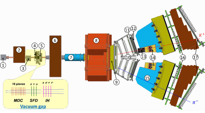
Figure 1: General view of the DIRAC setup (1 – target station; 2 – first shielding; 3 – micro drift chambers (MDC); 4 – scintillating fiber detector (SFD); 5 – ionization hodoscope (IH); 6 – second shielding; 7 – vacuum tube; 8 – spectrometer magnet; 9 – vacuum chamber; 10 – drift chambers (DC); 11 – vertical hodoscope (VH); 12 – horizontal hodoscope (HH); 13 – aerogel Cherenkov (ChA); 14 – heavy gas Cherenkov (ChF); 15 – nitrogen Cherenkov (ChN); 16 – preshower (PSh); 17 – muon detector (Mu).

After the target station, primary protons pass under the setup to the beam dump. The axis of the secondary channel is inclined relative to the proton beam by $5.7^{\circ}$ upward. The solid angle of the channel is $\Omega=1.2\cdot 10^{-3}$ sr. Secondary particles propagate mainly in vacuum up to the Al foil $(7.6\cdot 10^{-3}X_{0})$ at the exit of the vacuum chamber, which is installed between the poles of the dipole magnet ($B_{max}$ = 1.65 T and $BL$ = 2.2 Tm). In the vacuum channel gap, 18 planes of the Micro Drift Chambers (MDC) and ($X$, $Y$, $U$) planes of the Scintillation Fiber Detector (SFD) were installed in order to measure both the particle coordinates ($\sigma_{SFDx}=\sigma_{SFDy}=60$ µm, $\sigma_{SFDu}=120$ µm) and the particle time ($\sigma_{tSFDx}=380$ ps, $\sigma_{tSFDy}=\sigma_{tSFDu}=520$ ps). The total matter radiation thickness between target and vacuum chamber amounts to $7.7\cdot 10^{-2}X_{0}$. Each spectrometer arm is equipped with the following subdetectors [26]: drift chambers (DC) to measure particle coordinates with about 85 µm precision and to evaluate the particle path length; vertical hodoscope (VH) to determine particle times with 110 ps accuracy for identification of equal mass pairs via the time-of-flight (TOF) between SFDx plane and VH hodoscope; horizontal hodoscope (HH) to select in the two arms particles with a vertical distance less than 75 mm ($Q_{Y}$ less than 15 MeV/$c$); aerogel Cherenkov counter (ChA) to distinguish kaons from protons; heavy gas ($\text{C}_{4}\text{F}_{10}$) Cherenkov counter (ChF) to distinguish pions from kaons and protons; nitrogen Cherenkov (ChN) and preshower (PSh) detector to identify $e^{+}e^{-}$; iron absorber and two-layer scintillation counter (Mu) to identify muons. In the “negative” arm, no aerogel counter was installed, because the number of antiprotons is small compared to $K^{-}$.

Pairs of oppositely charged time-correlated particles (prompt pairs) and accidentals in the time interval $\pm$20 ns are selected by requiring a 2-arm coincidence (ChN in anticoincidence) with the coplanarity restriction (HH) in the first-level trigger. The second-level trigger selects events with at least one track in each arm by exploiting the DC-wire information (track finder). Particle pairs $\pi^{-}p$ ($\pi^{+}\bar{p}$) from $\Lambda$ ($\bar{\Lambda}$) decay were used for spectrometer calibration and $\text{e}^{+}\text{e}^{-}$ pairs for general detector calibration.

3 Fractions of $K^{+}K^{-}$ pairs with $K^{+}$ or $K^{-}$ mesons from the resonance decays

To study the $K^{+}K^{-}$ Coulomb and strong FSI one has to take into account a non point-like $K^{+}K^{-}$ pair production. Thus, if one hadron of the pair is a decay product of a relatively narrow resonance, the relative separation $r^{*}$ of the hadron production points may be substantially increased by the resonance path length $l^{*}$ in the pair c.m.s., which coincides at small $Q$ with the resonance path length in the rest frame of the decay hadron $l^{*}=p_{D}/(m_{h}\Gamma)$, where $p_{D}$ is the decay momentum of a hadron of mass $m_{h}$ and $\Gamma$ is the resonance width [33]. The path lengths of relatively narrow resonances such as $K^{*}(892)$ , $\Lambda(1520)$ and $\varphi(1020)$, are in $K^{+}K^{-}$ c.m.s. $2.3fm$, $6.2fm$ and $11.9fm$, respectively. They should be compared with $\langle r^{*}\rangle=(4/\pi)r_{0}\approx 4.5fm$ corresponding to a typical Gaussian radius $r_{0}\approx 2fm$, characterizing the $K^{+}K^{-}$ correlation function at moderate $Q$-values in $pA$ collisions, and the Bohr radius $r_{B}=110fm$. One may conclude that only the $\varphi(1020)$ path length substantially exceeds a typical $r^{*}$ separation.

Obviously, the increased separation due to the substantial resonance path length leads to a weaker Coulomb correlation than in the case of point-like pair production.

In order to take this into account, it is necessary to know the fractions of $K^{+}K^{-}$ pairs with $K^{+}$ or $K^{-}$ such resonance decays. The fractions of $K^{+}K^{-}$ pairs with $K^{+}$ or $K^{-}$ from the decays of $K(892)$, $\Lambda(1520)$ and $\phi(1020)$ were determined in [30] using the data on $K^{+}K^{-}$ pair production and cross sections of $K(892)$, $\Lambda(1520)$ and $\phi(1020)$ generation in pp interactions at 24GeV/c and 400GeV/c.

Other numerous resonances, some of which are observed only in the phase-shift analyses, either have large widths or small branching ratios into the final states with kaons and/or small production rates (such as $f_{1}(1285)$ with $\Gamma\approx 24MeV/c^{2}$ and $Br(K\bar{K})\approx 9\%$ or $f’(1525)$ with $\Gamma\approx 73MeV/c^{2}$ and $Br(K\bar{K})\approx 89\%$). The contribution of these resonances and direct $K^{+}K^{-}$ pairs to the distribution on $r^{*}$ will be described by a Gaussian.

The contributions of $K^{*}(892)$, $\Lambda(1520)$ and $\phi(1020)$ in $K^{+}K^{-}$ pairs production were evaluated as the product of the branching with generation of charged $K$ meson and the relative value of the dedicated inclusive cross section. Following [30] the relative contribution of all types of $K^{*}(892)$ equals to:

$$f_{K^{*}}(K^{+}K^{-})=(45\pm 10)\%$$ (1)

The fraction of $K^{+}K^{-}$ pairs with the $K^{-}$ from the $\Lambda(1520)$ decay amounts to:

$$f_{\Lambda(1520)}(K^{+}K^{-})=(8\pm 2)\%$$ (2)

The $K^{+}K^{-}$ pair from one and the same $\phi$ decay doesn’t contribute to $K^{+}K^{-}$ pairs at small $Q$. The contribution of $K$ meson from $\phi$ decay in the interval of small $Q$ is possible when $\phi$ is associated at least with a pair of strange particles (dominantly kaons). The cross sections of associated $\phi$ production measured at $24GeV/c$ and $400GeV/c$ are quite different, which may result from a bad kaon identification in the bubble chamber experiment at $24GeV/c$ and expected increase of the associated production with increasing energy, thus leading to a conservative estimate [30]:

$$f_{\phi}(K^{+}K^{-})=(2-14)\%$$ (3)

The errors in the $f$ values do not include the uncertainty of the approach used in [30]. Therefore, in the following we estimate the finite-size FSI effect on the $K^{+}K^{-}$ yield and $Q$ spectrum taking into account, besides a Gaussian short-distance contribution, also the ones containing exponential tails due to kaons from the decays of $K^{*}(890)$, $\Lambda(1520)$ and $\phi(1020)$ resonances using the fractions (1)-(3) to construct $r^{*}$ distributions with minimum and maximum values of average $r^{*}$.

4 Production of free $K^{+}K^{-}$ pairs

As mentioned in section 3 the prompt $K^{+}K^{-}$ pairs, emerging from proton-nucleus collisions, are produced manly from short-lived sources. These pairs undergo Coulomb and strong FSI resulting in modified unbound states (Coulomb pair) or forming bound systems. The accidental pairs arise from different proton-nucleus interactions.

4.1 Point-like $K^{+}K^{-}$ production and Coulomb FSI

Taking into account the Coulomb FSI only (Fig. 2 (a)), the production of unbound oppositely charged $K^{+}K^{-}$ pairs from short-lived sources, i.e. Coulomb pairs, is described [3] in the point-like production approximation, by

$$\frac{d^{6}\sigma_{C}}{d^{3}\vec{p}_{K^{+}}d^{3}\vec{p}_{K^{-}}}=\frac{d^{6}\sigma^{0}_{s}}{d^{3}\vec{p}_{K^{+}}d^{3}\vec{p}_{K^{-}}}A_{C}(q)\quad\mbox{with}\quad A_{C}(q)=\frac{2\pi m_{K}\alpha/q}{1-\exp\left(-2\pi m_{K}\alpha/q\right)}\;.$$ (4)

where $\vec{p}_{K^{+}}$ and $\vec{p}_{K^{-}}$ are the momenta of the charged kaons, $\sigma_{s}^{0}$ is the inclusive production cross section of $K^{+}K^{-}$ pairs from short-lived sources without FSI and the Coulomb enhancement function $A_{C}(q)$ represents the non-relativistic $K^{+}K^{-}$ Coulomb wave function squared at zero separation, well-known as the Gamov-Sommerfeld-Sakharov factor [18, 19, 20].

4.2 Non point-like $K^{+}K^{-}$ production and strong and Coulomb FSI

Up to now, the production of $K^{+}K^{-}$ pairs (4), was assumed to be point-like and only the Coulomb FSI was taken into account. The influence of the finite size effects and hadron strong interaction in the final state on the production of free and bound $K^{+}K^{-}$ pairs (Fig. 2 (b)), was considered in [15, 16, 34] and used to fit experimental $K^{+}K^{-}$ correlation functions in experiments NA49 [36], STAR [37] and ALICE [38].

As for the $K^{+}K^{-}$ strong interaction near threshold, it is dominated by the spin-0 isoscalar ($T=0$) and isovector ($T=1$) resonances $f^{0}(980)$ and $a^{0}(980)$ characterized by their masses $M_{r}$ and respective couplings $\gamma_{r}$ - to the $K{\bar{K}}$ channel and $\gamma_{r}\,^{\prime}$ - to the $\pi\pi$ and $\pi\eta$ channels for $f^{0}(980)$ and $a^{0}(980)$, respectively [34], [35], [38], [40], [41], [42].

There is a great deal of uncertainty in the properties of these resonances reflected in uncertainties of their PDG widths: $10-100MeV$ and $50-100$ MeV for $f^{0}(980)$ and $a^{0}(980)$, respectively. Fortunately, the dominant imaginary parts of the scattering lengths are basically determined by the ratios $\gamma_{r}/\gamma_{r}\,^{\prime}$ with rather small uncertainty. As for the real parts of the scattering lengths, due to the closeness of $f^{0}$ and $a^{0}$ masses to the $K\bar{K}$ threshold, they are quite uncertain and rather small, varying in existing fits from $-0.3fm$ to $0.3fm$.

To calculate the $K^{+}K^{-}$ correlation function, we use the $f^{0}(980)$ and $a^{0}(980)$ parameters from Martin et al.[40], Achasov et al. [41] and ALICE [38]. The ALICE parameters for $a^{0}(980)$ coincide with those from Achasov et al., and, for $f^{0}(980)$, they are determined from a fit of the ALICE $K^{+}K^{-}$ correlation functions.

Note that the ALICE $K^{+}K^{-}$ correlation data [38] disagrees with the $f^{0}(980)$ parameterisations from Martin et al.[40], Achasov et al.[41], and Antonelli [42]. The ALICE $K_{s}\,K^{\pm}$ correlation data [43] (with the absent $f^{0}$ contribution) excludes $a^{0}(980)$ parameters from Martin et al., favouring those from Achasov et al., while the STAR and ALICE $K_{s}\,K_{s}$ correlation data [35, 39], is unable to discriminate among all these parameterizations.

(a)	(b)

Figure 2: The schematic description of $K^{+}K^{-}$ production processes. a) The black point presents the pair point-like production; the wavy lines describe the Coulomb interaction in the final state. b) The circle and square present the pair non point-like production and strong interaction in the final state respectively.

5 Data processing

The collected events were analyzed with the DIRAC reconstruction program ARIANE [32] modified for analyzing $KK$ data.

5.1 Tracking

Only events with one or two particle tracks in DC of each arm are processed. The event reconstruction is performed according to the following steps [14]:

• One or two hadron tracks are identified in DC of each arm with hits in VH, HH and PSh slabs and no signal in ChN and Mu.

• Track segments, reconstructed in DC, are extrapolated backward to the beam position in the target, using the transfer function of the dipole magnet and the program ARIANE. This procedure provides approximate particle momenta and the corresponding points of intersection in MDC, SFD and IH.

• Hits are searched for around the expected SFD coordinates in the region $\pm 1$ cm corresponding to (3–5) $\sigma_{\text{pos}}$ defined by the position accuracy taking into account the particle momenta. The number of hits around the two tracks is $\leq 4$ in each SFD plane and $\leq 9$ in all three SFD planes. In some cases only one hit in the region $\pm 1$ cm occurred. To identify the event when two particles crossed the same SFD column was requested the double ionisation in the corresponding IH slab.

The momentum of the positively or negatively charged particle is refined to match the $X$-coordinates of the DC tracks as well as the SFD hits in the $X$- or $U$-plane, depending on the presence of hits. In order to find the best 2-track combination, the two tracks may not use a common SFD hit in the case of more than one hit in the proper region. In the final analysis, the combination with the best $\chi^{2}$ in the other SFD planes is kept.

5.2 Setup tuning using $\Lambda$ and $\bar{\Lambda}$ particles

In order to check the general geometry of the DIRAC experiment, the $\Lambda$ and $\bar{\Lambda}$ particles, decaying into ${\rm p}\pi^{-}$ and $\pi^{+}\bar{\rm p}$ in our setup, were used [14]. After setup tuning the weighted average value of the experimental $\Lambda$ mass over all runs, $M^{\mathrm{DIRAC}}_{\Lambda}=(1.115680\pm 2.9\cdot 10^{-6})$ GeV/$c^{2}$, agrees very well with the PDG value, $M^{\mathrm{PDG}}_{\Lambda}=(1.115683\pm 6\cdot 10^{-6})$ GeV/$c^{2}$. The weighted average of the experimental ${\bar{\Lambda}}$ mass is $M^{\mathrm{DIRAC}}_{\bar{\Lambda}}=(1.11566\pm 1\cdot 10^{-5})$ GeV/$c^{2}$. This demonstrates that the geometry of the DIRAC setup is well described.

The width of the $\Lambda$ mass distribution allows to test the momentum and angular setup resolution in the simulation. Table 1 shows a good agreement between simulated and experimental $\Lambda$ width in DATA1 and DATA2. A further test consists in comparing the experimental $\Lambda$ and ${\bar{\Lambda}}$ widths.

Table 1: $\Lambda$ width in GeV/$c^{2}$ for experimental and MC data and ${\bar{\Lambda}}$ width for experimental data.

	$\Lambda$ width (data)	$\Lambda$ width (MC)	${\bar{\Lambda}}$ width (data)
	GeV/$c^{2}$	GeV/$c^{2}$	GeV/$c^{2}$
DATA1	$4.42\cdot 10^{-4}\pm 7.4\cdot 10^{-6}$	$4.42\cdot 10^{-4}\pm 4.4\cdot 10^{-6}$	$4.5\cdot 10^{-4}\pm 3\cdot 10^{-5}$
DATA2	$4.41\cdot 10^{-4}\pm 7.5\cdot 10^{-6}$	$4.37\cdot 10^{-4}\pm 4.5\cdot 10^{-6}$	$4.3\cdot 10^{-4}\pm 2\cdot 10^{-5}$

The average value of correction which was introduced in the simulated width is $1.00203\pm 0.00191\cdot 10^{-3}$. This number to be used for the introduction of the non significant corrections in the l.s. particle’s momenta.

The $Q_{L}$ distribution of $\pi^{+}\pi^{-}$ pairs can be used to check the geometrical alignment. Since the $\pi^{+}\pi^{-}$ system is symmetric, the corresponding $Q_{L}$ distribution should be centered at 0. The experimental $Q_{L}$ distribution of pion pairs with transverse momenta $Q_{T}<4$ MeV/$c$, is centered at 0 with a precision of 0.2 MeV/$c$.

5.3 Event selection

The processed events were collected in DATA1 and DATA2. Equal mass pairs contained in the selected event sample are classified into three categories: $K^{+}K^{-}$, $\pi^{+}\pi^{-}$ and $p\bar{p}$ pairs.

The classification is based on the TOF measurement [44]. In the momentum range from 3.8 to 7 $\text{GeV}/c$, additional information from the Heavy Gas Cherenkov (ChF) counters (Section 2) is used to better separate $\pi^{+}\pi^{-}$ from $K^{+}K^{-}$ and $p\bar{p}$ pairs. The ChF counters detect pions in this region with (95–97)% efficiency [31], whereas kaons and protons (antiprotons) do not generate any signal. Due to the finite resolution of the TOF system and the Cherenkov efficiency, the selected $K^{+}K^{-}$ sample with high momentum pairs still contains about 10% $\pi^{+}\pi^{-}$ and 10% $p\bar{p}$ events.

The TOF is measured and calculated for the distance between the SFD X-plane and the VH of about 11m. The length and momentum of each track are evaluated using the tracking system. The relative precision of the momentum measurement is about $3\times 10^{-3}$. For ’positive’ and ’negative’ tracks, the expected TOF $t^{calc}_{\pm}$ is calculated assuming that it is $K^{+}K^{-}$ pair. Furthermore, the difference between calculated and measured TOF, $\Delta t_{\pm}=t^{calc}_{\pm}-t^{exp}_{\pm}$, was determined. In order to classify the pairs, the averaged difference $\Delta t=\frac{1}{2}(\Delta t_{+}+\Delta t_{-})$ was used. The $\Delta t^{K}$ distribution of events corresponding to a momentum of about 3.5$\text{GeV}/c$ is presented in Fig. 3.

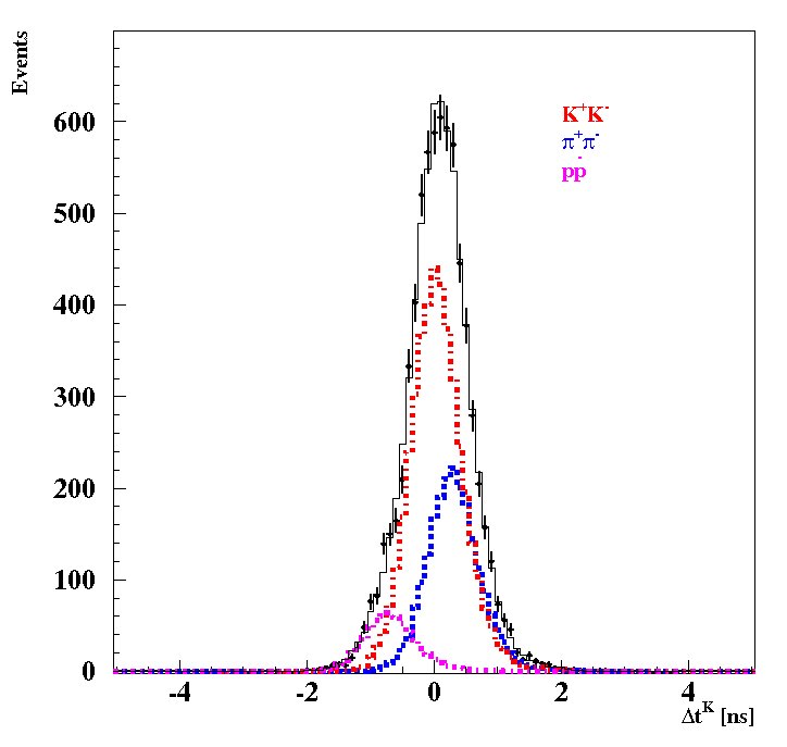
Figure 3: $\Delta t^{K}$ distribution of $K^{+}K^{-}$, $\pi^{+}\pi^{-}$ and $p\bar{p}$ pairs with momentum of about 3.5$\text{GeV}/c$. The peak at zero corresponds to $K^{+}K^{-}$, the peak on the right to $\pi^{+}\pi^{-}$ and the small peak on the left to $p\bar{p}$ pairs.

To evaluate the amount of pairs in each category, model distributions of $\Delta t^{K}$ obtained from $e^{+}e^{-}$ pairs are used [44]. These $e^{+}e^{-}$ data were collected for calibration purposes with a dedicated trigger (Section 2) during standard data taking. Again, the average difference $\Delta t^{e}$ between expected and measured TOF for the electron and positron was calculated assuming electron mass. The $\Delta t^{e}$ distribution shown in Fig. 4 exhibits a half width at half maximum of 440 ps corresponding to the time resolution of the TOF system.

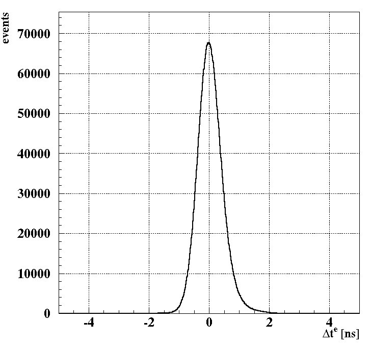
Figure 4: $\Delta t^{e}$ distribution of electron-positron pairs.

The $\Delta t^{K}$ distributions of $K^{+}K^{-}$, $\pi^{+}\pi^{-}$ and $p\bar{p}$ pairs at fixed lab momentum $p_{lab}$ show the same shape as for $e^{+}e^{-}$. The $K^{+}K^{-}$ peak is at zero, whereas the $\pi^{+}\pi^{-}$ and $p\bar{p}$ peaks are on the positive and negative side, respectively. The distance of the $\pi^{+}\pi^{-}$ and $p\bar{p}$ peak from zero is increasing with decreasing $p_{lab}$.

The experimental data are spread over a wide momentum interval (2.5–7) GeV/$c$. The shape of the $\Delta t^{K}$ distribution depends on momentum and on its interval width. Therefore, the data are analyzed within bins of a new variable $\Delta T_{K-\pi}$. For each track in a pair, the $\Delta t$ parameter was calculated in two versions: 1) using kaon mass ($\Delta t^{K}$) and 2) using pion mass ($\Delta t^{\pi}$). The new parameter $\Delta T_{K-\pi}$ is then defined as the difference between the TOFs calculated for kaon and pion (for each pair track):

$$\Delta T_{K-\pi}=\frac{1}{2}(\Delta T^{+}_{K-\pi}+\Delta T^{-}_{K-\pi})=\Delta t^{K}-\Delta t^{\pi}.$$ (5)

In the analysis, the data are processed in one hundred 25 ps wide $\Delta T_{K-\pi}$ bins.

The advantage of this technique is the constant shape of the $\Delta t^{K}$ distribution of $\pi^{+}\pi^{-}$ and $K^{+}K^{-}$ pairs for different $\Delta T_{K-\pi}$ values. The selection of a particular $\Delta T_{K-\pi}$ bin fixes the distance between the peak positions of the distributions corresponding to $K^{+}K^{-}$ and $\pi^{+}\pi^{-}$ pairs. The distance $\Delta T_{K-\pi}$ between the peaks of the $K^{+}K^{-}$, $\pi^{+}\pi^{-}$ and $p\bar{p}$ pairs is maximal for pairs with minimal momentum $p^{min}_{lab}=2.5$GeV/$c$.

The model distributions of $\pi^{+}\pi^{-}$, $K^{+}K^{-}$ and $p\bar{p}$ pairs are used to fit the experimental distributions. In each 25 ps $\Delta T_{K-\pi}$ bin, the amount of events is determined for the three categories as shown in Fig. 3. The collected data consists mainly of $\pi^{+}\pi^{-}$ pairs. For analyzing $K^{+}K^{-}$ pairs, subsets with a significant $K^{+}K^{-}$ portion are needed. In each $\Delta T_{K-\pi}$ bin, contiguous bins in $\Delta t^{K}$ are selected by demanding the $K^{+}K^{-}$ population to exceed a certain threshold. Hence, we consider three subsamples of events containing at least a $K^{+}K^{-}$ population of 30%, 50% and 70%. The cleanest so-called 70% $K^{+}K^{-}$ sample consists of only $K^{+}K^{-}$ pairs with high momenta, where Cherenkov counters suppress $\pi^{+}\pi^{-}$ pairs efficiently.

6 Experimental results

For DATA1 and DATA2, the $K^{+}K^{-}$, $\pi^{+}\pi^{-}$ and $p\bar{p}$ pair numbers were evaluated in the 30%, 50% and 70% subsample (Table 2). The number of proton interaction with the target in DATA1 and DATA2 are nearly the same.

Table 2: Pair numbers in DATA1 and DATA2, evaluated in the three subsamples (30%, 50%, 70%). The $R$ is the ratio of events in correspondent subsample to the full number (all).

DATA1	Experimental data ($Q_{T}<15~{}\rm{MeV}/c$)				$R$ (%)
Sample	all	30%	50%	70%	30%/all	50%/all	70%/all
$\pi^{+}\pi^{-}$	$7.77\cdot 10^{6}$	17290	3540	620	0.22	0.05	0.008
$K^{+}K^{-}$	90840	25660	15040	8210	28.2	16.6	9.0
$p\bar{p}$	7670	2960	1930	880	38.6	25.2	11.5

DATA2	Experimental data ($Q_{T}<15~{}\rm{MeV}/c$)				$R$ (%)
Sample	all	30%	50%	70%	30%/all	50%/all	70%/all
$\pi^{+}\pi^{-}$	$7.96\cdot 10^{6}$	15230	2970	80	0.19	0.04	0.001
$K^{+}K^{-}$	92960	25550	15910	8330	27.5	17.1	9.0
$p\bar{p}$	7200	2950	1780	770	41.0	24.7	10.7

It can be seen that the number of $K^{+}K^{-}$ pairs in DATA1 and DATA2 without cutting in the three subsamples are consistent. The experimental data were obtained with a trigger restriction on $Q_{T}$ at about 15 MeV/$c$. For the final analysis, data were used with the software restriction $Q_{T}<6$ MeV/$c$, where the setup efficiency is constant. To study a possible influence of the $Q_{T}$ limit on $R$, a larger data sample with $Q_{T}<8$ MeV/$c$ was also analyzed. The resulting pair numbers for $Q_{T}<8$ MeV/$c$ are decreased by 1.8 and the corresponding $R$ values in agreement with those in Table 2.

All events in the three samples are prompt. Their numbers and distributions on any parameter were evaluated by subtracting the background of the accidental events using the time difference between VH hodoscopes. The percentage of accidentals before subtraction in the 70%, 50% and 30% samples was 9.6%, 22% and 47%, respectively. The 70% sample is the most reliable for the $K^{+}K^{-}$ pair analysis, because the total background of accidentals, $\pi^{+}\pi^{-}$ and $p\bar{p}$ prompt pairs is significantly smaller than in the two other samples. After background subtraction, the $K^{+}K^{-}$ purity is the highest one.

6.1 The simulation procedure

The experimental distributions of $K^{+}K^{-}$ pairs were compared with the corresponding simulated spectra according to different theoretical models. The simulated $K^{+}K^{-}$ spectra in the pair c.m.s. were calculated using the relation:

$$\frac{dN}{dQ_{i}}=|M_{prod}|^{2}F(Q_{i})F_{corr}(Q_{i})$$ (6)

where $Q_{i}$ is $Q$ or $Q_{L}$, $M_{prod}$ the production matrix element without the $Q$ dependence in the investigated $Q$ interval, $F(Qi)$ the phase space and $F_{corr}(Q_{i})$ the correlation function. This function takes into account the Coulomb FSI in the Coulomb approximation ($A_{c}(Q)$) or the Coulomb and strong FSI in the more precise models. For the c.m.s. pair is added the l.s. momentum $\vec{P}_{lab}$ that allows to calculate the $\vec{P}^{+}$ and $\vec{P}^{-}$ momentua of the $K^{+}$ and $K^{-}$ in l.s and their total momentum $\vec{P}=\vec{P}^{+}+\vec{P}^{-}$.

By means of the dedicated code GEANT-DIRAC, the simulated pairs are propagated through the setup, taking into account multiple scattering, the response of the detectors before the magnet on the $K^{+}K^{-}$ pairs and the response of the detectors after magnet on the single particle. Using the information from the detectors the events were reconstructed by the code ARIANE and processed as experimental pairs. Then, their $Q_{L}$ and $Q$ distributions were calculated and compared with the corresponding experimental spectra. The $\vec{P}_{lab}$ distribution was obtained by requiring that $\vec{P}$ spectrum must fit the experimental $K^{+}K^{-}$ pair spectrum in $\vec{P}_{exp}=\vec{P}^{+}_{exp}+\vec{P}^{-}_{exp}$ where $\vec{P}^{+}_{exp}$ and $\vec{P}^{-}_{exp}$ are experimental l.s. momentum of $K^{+}$ and $K^{-}$.

6.2 Analysis of $Q_{L}$ and $Q$ distributions

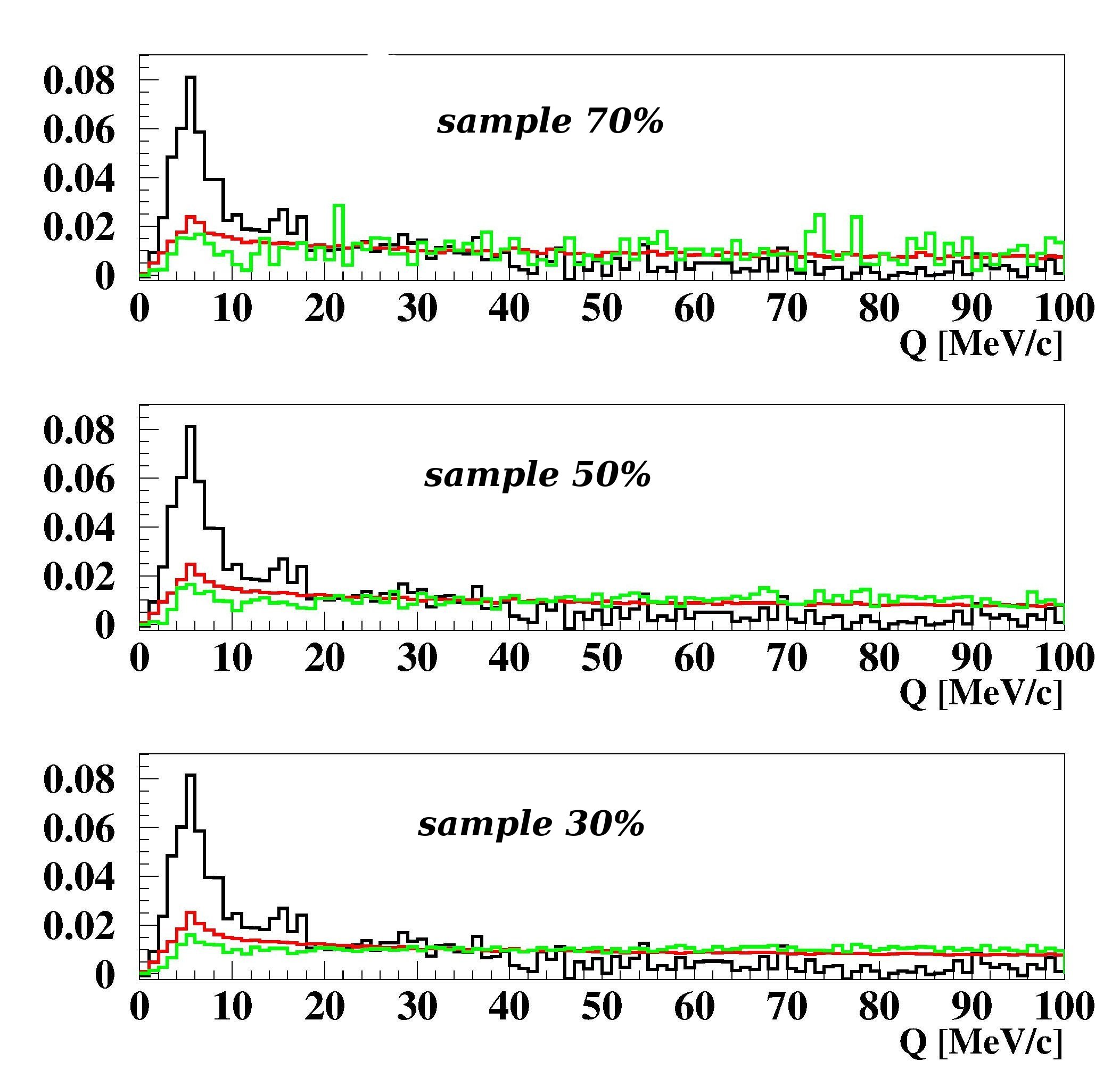
Figure 5: The $Q$ distribution of $\pi^{+}\pi^{-}$ (red), $p\bar{p}$ (black) and accidentals (green) pairs calculated as $K^{+}K^{-}$ pairs.

The subtraction of $\pi^{+}\pi^{-}$, $p\bar{p}$ and accidentals background is based on the estimated time and momentum setup resolutions. A statistical fluctuation and possible systematic uncertainty of this subtraction may lead to a residual background, distorting the $K^{+}K^{-}$ distributions in $Q$ and $Q_{L}$. The fractions of $K^{+}K^{-}$ and residual background pairs can be evaluated using different shapes of their $Q$ and $Q_{L}$ distributions.

The distributions of accidentals and $\pi^{+}\pi^{-}$ pairs were obtained calculating these experimental pairs as $K^{+}K^{-}$ system for each subsample. Due to small yield of $p\bar{p}$ pairs only one sample containing bins with their population greater than $50\%$ was produced. The $p\bar{p}$ sample was processed as $K^{+}K^{-}$ system and used for all three subsamples analysis. The $Q$ spectra of the three background types for all subsamples are shown in Fig.5.

Taking into account a small difference between the shapes of $\pi^{+}\pi^{-}$ and accidental background distributions, we fit the $K^{+}K^{-}$ and residual background fractions, assuming the same shape of $\pi^{+}\pi^{-}$ and accidental background $Q$ and $Q_{L}$ distributions, i.e., considering the $\pi^{+}\pi^{-}$ and $p\bar{p}$ background only.

The effect and background values must not depend from the distribution type chosen. To check it the dedicated analysis was done for $Q$ and $Q_{L}$ experimental distributions using fitting curve and only $\pi^{+}\pi^{-}$ and $p\bar{p}$ background. In this analysis the $K^{+}K^{-}$ pairs distribution in $Q$, $Q_{L}$ is calculated proposing the point-like $K^{+}K^{-}$ pairs production with only Coulomb interaction in the final state (Coulomb parametrization). For each run and each subsample, the experimental $Q$, $Q_{L}$ distributions $D_{exp}$ were fitted by sum of the three distributions according to the formula:

$$D_{exp}=N_{KK}D_{KK}^{n}+N_{\pi\pi}D_{\pi\pi}^{n}+N_{p\bar{p}}D_{p\bar{p}}^{n}$$ (7)

where $D_{\pi\pi}^{n}$ and $D_{p\bar{p}}^{n}$ denote corresponding background distributions of $\pi^{+}\pi^{-}$ and $p\bar{p}$ pairs normalized to unity, $D_{KK}^{n}$ is the simulated $K^{+}K^{-}$ distribution normalized to unity. $N_{\pi\pi}$ and $N_{p\bar{p}}$ are free fitted parameters indicating number of $\pi^{+}\pi^{-}$ and $p\bar{p}$ pairs.

The number of $K^{+}K^{-}$ pairs, $N_{KK}$, is given by the constraint

$$N_{exp}=N_{KK}+N_{\pi\pi}+N_{p\bar{p}}$$ (8)

where $N_{exp}$ is the total number of events in given $D_{exp}$ distribution. In this case the errors of the $K^{+}K^{-}$ pairs and total background number are equal.

For the six distributions on $Q$ and $Q_{L}$ (DATA1 and DATA2, three subsamples) all the $\chi^{2}/\mathrm{ndf}$ values are within the interval 0.7-1.2, and the $K^{+}K^{-}$ numbers of the two runs in each subsample are in agreement. The $\chi^{2}/\mathrm{ndf}$ values for $Q$ distributions in DATA2/DATA1 runs are $0.98/1.19,0.77/1.08$ and $0.69/0.87$ for 70%, 50% and 30% subsamples respectively. The probability density function (PDF) has maximum around $\chi^{2}/\mathrm{ndf}=1$ and decreased by half for $\chi^{2}/\mathrm{ndf}=0.85$ and $1.15$. The Coulomb parametrization describes all 6 experimental distributions well because the PDF values for 70% and 50% subsamples for two data sets are near maximum at $\chi^{2}/\mathrm{ndf}\approx 1$ and for 30% subsample this parameter is near maximum for DATA2 and for DATA1 it deflects from maximum with 0.31 value, which is acceptable.

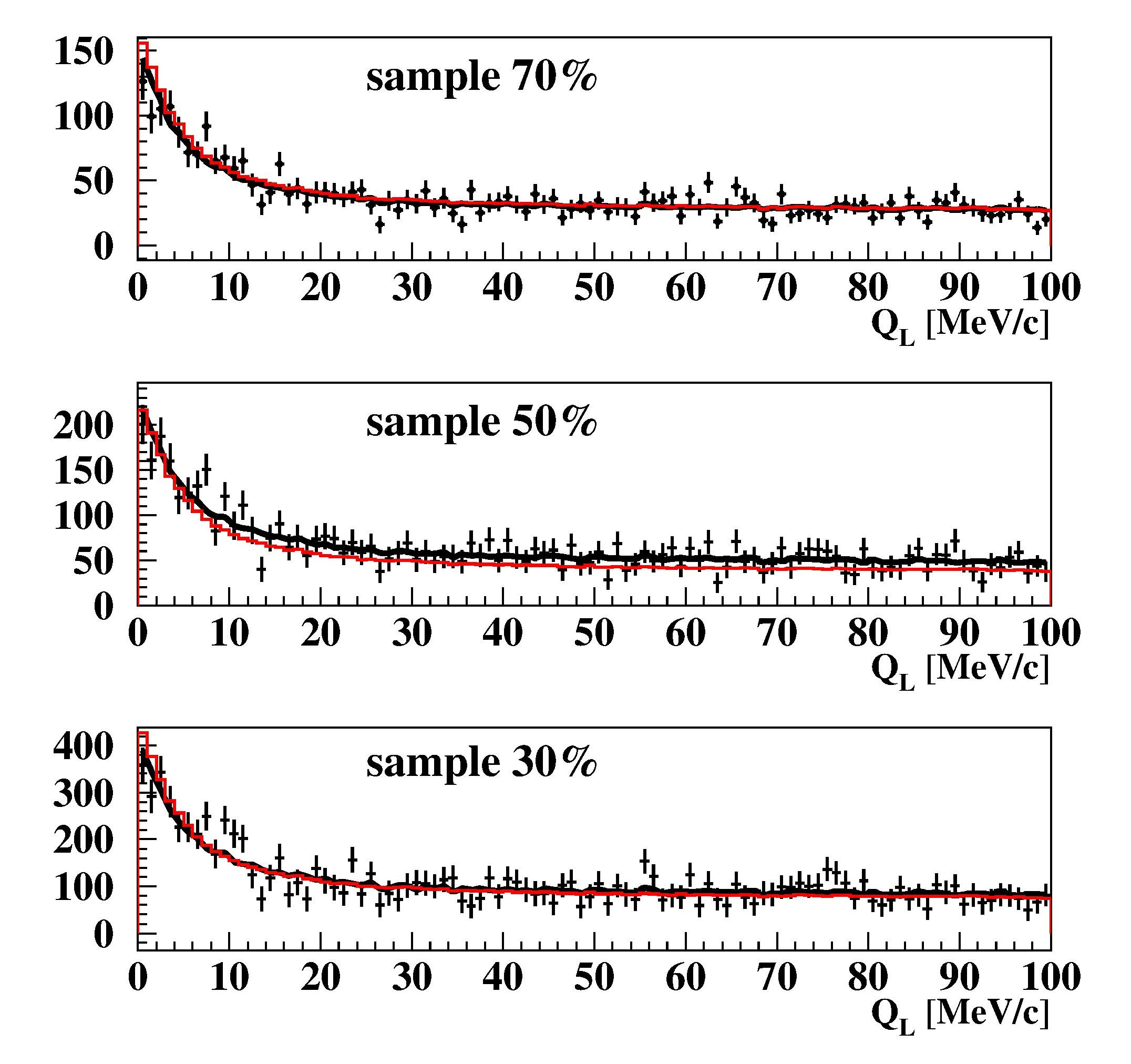
Figure 6: $Q_{L}$ distributions of the subsamples 30%, 50% and 70% for DATA1 and DATA2. The experimental spectra in the interval $0<Q_{L}<100$ MeV/c are fitted by simulated $K^{+}K^{-}$ (point-like Coulomb FSI) and residual $\pi^{+}\pi^{-}$ and $p\bar{p}$ background distributions. The red curve is the $K^{+}K^{-}$ distribution, the black one is the sum of $K^{+}K^{-}$ and residual background distributions. In the subsamples 70% and 30% the residual background is small and these curves practically coincide. For $K^{+}K^{-}$ pairs in the region of $Q_{L}<10$ MeV/c the Coulomb enhancement is clearly visible, whereas the residual background is small.

Figure 6 presents the experimental distributions in $Q_{L}$, the fitting curves for $K^{+}K^{-}$ pairs and the sum of the total background and fitting distributions. It is seen that in the 70% and 30% subsamples the fitting curves coincide practically with the experimental distributions demonstrating that the residual background is small. In the 50% subsample the background level is significantly higher and the fitting curve is lower than the experimental points.

A strong enhancement in the pair yield can be recognized in the $Q_{L}$ distributions between 0 to 10 MeV/c. It is caused by the Coulomb final state $K^{+}K^{-}$ pairs interaction, because the residual background is small. The same analysis was performed for $Q$ distributions.

Table 3 presents the outcome of the two analyses and demonstrates a good agreement for the $K^{+}K^{-}$ pair numbers obtained in the $Q_{L}$ and $Q$ distribution analysis.

The $K^{+}K^{-}$ pair numbers presented in Table 3 were obtained with the residual background description using only $\pi^{+}\pi^{-}$ and $p\overline{p}$ pairs. The fits, where accidental background was added, to give the same numbers of $K^{+}K^{-}$ pairs within 0-0.2 errors.

Table 3: Matching pair numbers for $Q$ and $Q_{L}$ distribution analyses. The errors of $K^{+}K^{-}$ and background values are the same.

	cut on ToF	distribution	$K^{+}K^{-}$	$\pi^{+}\pi^{-}$ & $p\bar{p}$ background
DATA1 + DATA2	$70\%$	$Q$	$3900\pm 410$	$-110$
		$Q_{L}$	$3930\pm 580$	$-140$
	$50\%$	$Q$	$5320\pm 730$	$1100$
		$Q_{L}$	$5460\pm 1020$	$960$
	$30\%$	$Q$	$11220\pm 1370$	$180$
		$Q_{L}$	$10750\pm 2020$	$300$

6.3 Data analysis assuming non point-like $K^{+}K^{-}$ pair production and Coulomb and strong $K^{+}K^{-}$ interaction in the final state

In section 6.2 the $K^{+}K^{-}$ pairs were analyzed assuming their point-like production and taking into account only Coulomb interaction in the final state. In this section the $K^{+}K^{-}$ distributions in $Q$ will be analyzed taking into account non point-like pairs production and their Coulomb and strong interactions in the final state. It will use three theoretical parametrizations: Achasov et al.[41], Martin et al.[40] and ALICE [38].

The distribution in the distance $r^{*}$ between two $K$ mesons in the general case is presented as the sum of four distributions in $r^{*}$ connecting the $K$ mesons from the decay of short-lived sources and long-lived resonances:

$$w_{g}*Gauss+w_{K^{*}}*K^{*}(892)+w_{\Lambda}*\Lambda(1520)+w_{\varphi^{*}}*\varphi(1020)$$ (9)

The first term describes the contributions of the short-lived sources approximated by Gaussian with the radius $r_{0}\approx 1.5fm$, the other terms describe the contributions of the three resonances. The $w_{i}$ are the relative contributions of the different sources in $K^{+}K^{-}$ pair production. The weights values were evaluated using the numbers and their errors presented in the equations (1), (2), (3) and the requirement that the sum of $w_{i}$ equals unity.

The analysis was performed for the three sets of $w_{i}$. The first extreme set (0.00, 0.76, 0.10, 0.14) maximizes the contributions of $K^{*}(892)$, $\Lambda(1520)$ and $\varphi(1020)$ resonances producing the largest value of average $r^{*}$; the third extreme set (0.57, 0.35, 0.06, 0.02) maximizes the role of the short-lived $K^{+}K^{-}$ pairs sources generating the minimum value of the average $r^{*}$ and the second set (0.10, 0.76, 0.08, 0.06) is using the intermediate values of $w_{i}$. The $Q$ distribution (fitting curves) were calculated for each of DATA1, DATA2 and for each sample, using three theoretical parametrizations of Achasov, Martin and ALICE [38, 40, 41].

The experimental data of the 70% subsample was analyzed by dedicated fitting curve with $\pi^{+}\pi^{-}$ and $p\bar{p}$ background. The results obtained are shown in Table 4. The background errors are the same as for $K^{+}K^{-}$ pairs. The $K^{+}K^{-}$ pairs yield is increasing with enlarging $r^{*}$ value. The difference between extreme yields values gives the maximum numbers of systematic errors in connection with the uncertainty of $r^{*}$ distribution. The errors values are $\pm 70,\pm 55$ and $\pm 40$. These systematic errors are significantly smaller than the errors in Table 4. Therefore for the analysis of the two other experimental subsamples, we will use only the intermediate $r^{*}$ distribution. The results of the 70%, 50% and 30% subsamples are presented in Table 4.

Table 4: Pair numbers in the DATA1 and DATA2. The number of $K^{+}K^{-}$ and background pairs (in brackets) were evaluated by fitting experimental distributions on $Q$ in three subsamples by $K^{+}K^{-}$ distributions, calculated with different parametrizations. The errors of $K^{+}K^{-}$ and background pairs are identical.

	Achasov	Martin	ALICE	Total
	$K^{+}K^{-}$ (backgr.)	$K^{+}K^{-}$ (backgr.)	$K^{+}K^{-}$ (backgr.)	events
70% sample				3790
maximum $r^{*}$	$3190\pm 330$	$3650\pm 370$	$3720\pm 380$
intermediate $r^{*}$	$3120\pm 320$ (670)	$3600\pm 360$ (190)	$3680\pm 370$ (110)
$\chi^{2}/\mathrm{ndf}$ DATA2/DATA1	$1.03/1.20$	$1.00/1.18$	$1.00/1.18$
minimum $r^{*}$	$3050\pm 320$	$3540\pm 360$	$3640\pm 370$
50% sample				6420
intermediate $r^{*}$	$4340\pm 570$ (2080)	$4940\pm 640$ (1480)	$5040\pm 660$ (1380)
$\chi^{2}/\mathrm{ndf}$ DATA2/DATA1	$0.80/1.04$	$0.79/1.04$	$0.78/1.05$
30% sample				11030
intermediate $r^{*}$	$9230\pm 1080$ (1800)	$10500\pm 1220$ (530)	$10680\pm 1240$ (350)
$\chi^{2}/\mathrm{ndf}$ DATA2/DATA1	$0.70/0.89$	$0.68/0.88$	$0.68/0.88$

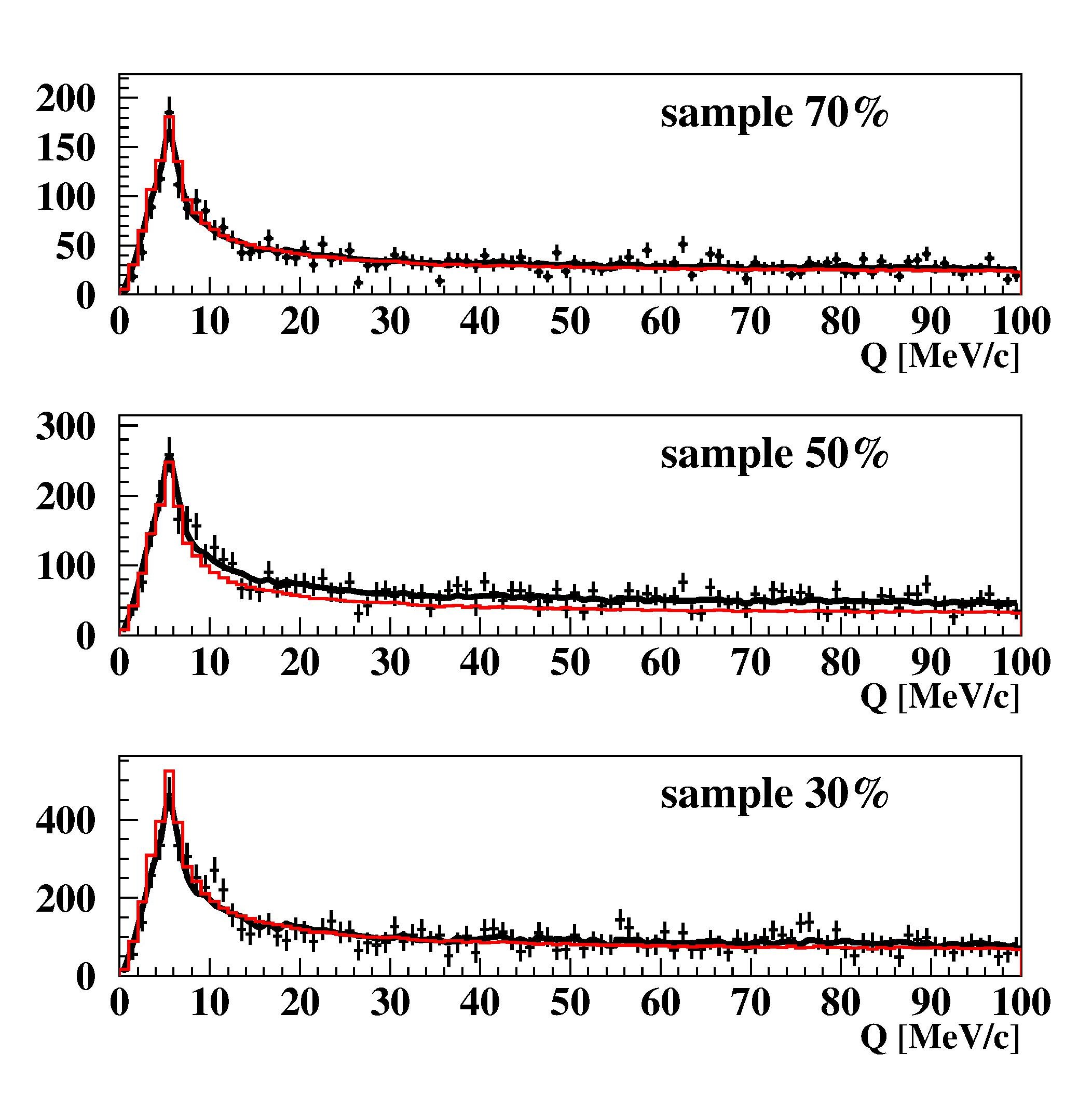
Figure 7: $Q$ distributions of the subsamples 30%, 50% and 70% for DATA1 and DATA2. Simulated distributions of $K^{+}K^{-}$ (ALICE parametrization) and residual background of $\pi^{+}\pi^{-}$, accidental and $p\bar{p}$ pairs are fitting the experimental spectrum in the interval $0<Q<100~{}MeV/c$. The red line is the $K^{+}K^{-}$ distribution, the black line is the sum of $K^{+}K^{-}$ and residual background. In the subsamples 70% and 30% the residual background is small and these lines practically coincide.

It is seen from Table 4 that for any subsample the Achasov parametrization gives the residual background deflection from zero significantly larger than Martin and ALICE calculations. The large level of residual background can be considered as a result of insufficient accuracy of the fitting curve describing $K^{+}K^{-}$ distribution on $Q$. The additional reason for the better precision of Martin and ALICE parametrization can be obtained from the residual background estimation. The expected numbers of $\pi^{+}\pi^{-}$, $p\bar{p}$ and accidental pairs in 70%, 50% and 30% subsamples are $1050\pm 50$, $5300\pm 120$ and $30370\pm 630$ respectively. The errors include the systematical and statistical accuracy of the expected background level evaluation and background statistical fluctuations. After expected background subtraction the real residual background can differ from zero to one-three errors.

In Achasov parametrization in the 70% subsample the background deflection is 13 standard deviations. In the same subsample the respective deviations for Martin and ALICE parametrizations are 3.8 (2.2) standard deviations. Therefore in the present paper the experimental data will be analyzed using as a main ALICE and Martin parametrizations.

The large residual background in the 50% subsample indicates that this experimental distribution is less reliable than the 70% subsample which will be used for the calculation of the $K^{+}K^{-}$ pairs total number. The $\chi^{2}/\mathrm{ndf}$ values of Martin and ALICE parametrizations for 70% and 50% subsamples are slightly better than the same quantities obtained using Coulomb parametrization. It shows that experimental data precision is not enough to choose, using $\chi^{2}/\mathrm{ndf}$ values, between simple description using point-like production and only Coulomb FSI and more precise theoretical approaches taking into account non point-like pairs production, Coulomb and strong FSI. In the future analysis the Martin and ALICE results obtained with a more accurate theoretically approach will be used.

Figure 7 shows the experimental distributions in $Q$, fitting curves describing $K^{+}K^{-}$ pairs (ALICE parametrization) and sum of fitting curves and residual backgrounds. It is seen that for 70% (30%) subsample the fitting curve alone describes well the experimental distribution in the total interval of $Q$ demonstrating that admixture of the residual background to the $K^{+}K^{-}$ pairs is relatively small. This result is in agreement with the average level of residual background, it equals 3% (3.2%) of the total number of events in the distribution. The same analysis was done for the 50% subsample.

6.4 Evaluation of the total number of detected $K^{+}K^{-}$ pairs

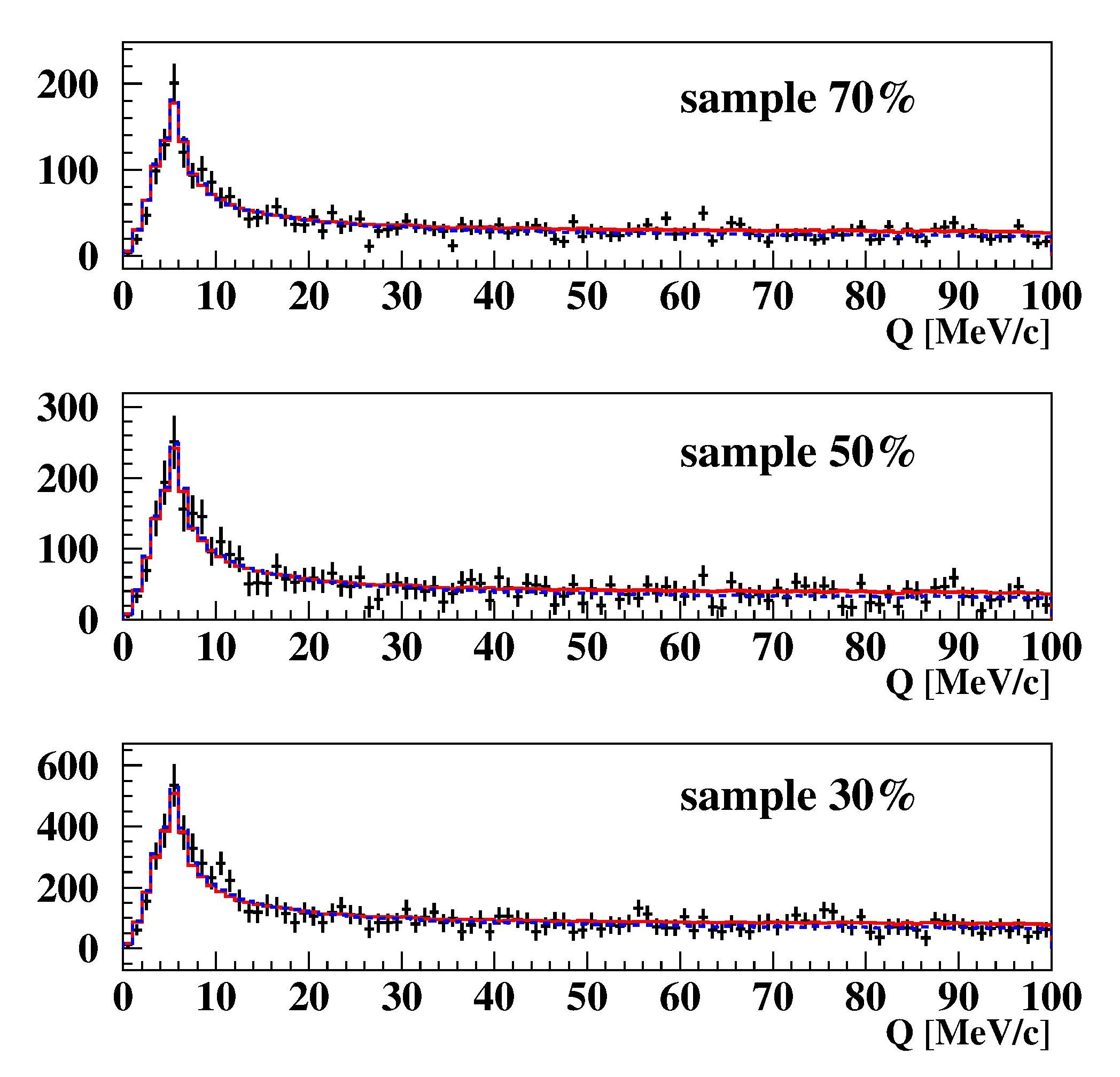
Figure 8: $Q$ distributions in the interval $0-100~{}MeV/c$ of $K^{+}K^{-}$ (ALICE parametrization) of the subsamples 30%, 50% and 70% for the DATA1 and DATA2 after residual background subtraction. The red and the blue fitting curves were evaluated from the analysis of experimental distributions with residual background in Coulomb and Martin parametrizations respectively. It is seen that the difference between these curves is not significant and they describe ”pure” experimental $K^{+}K^{-}$ distributions well.

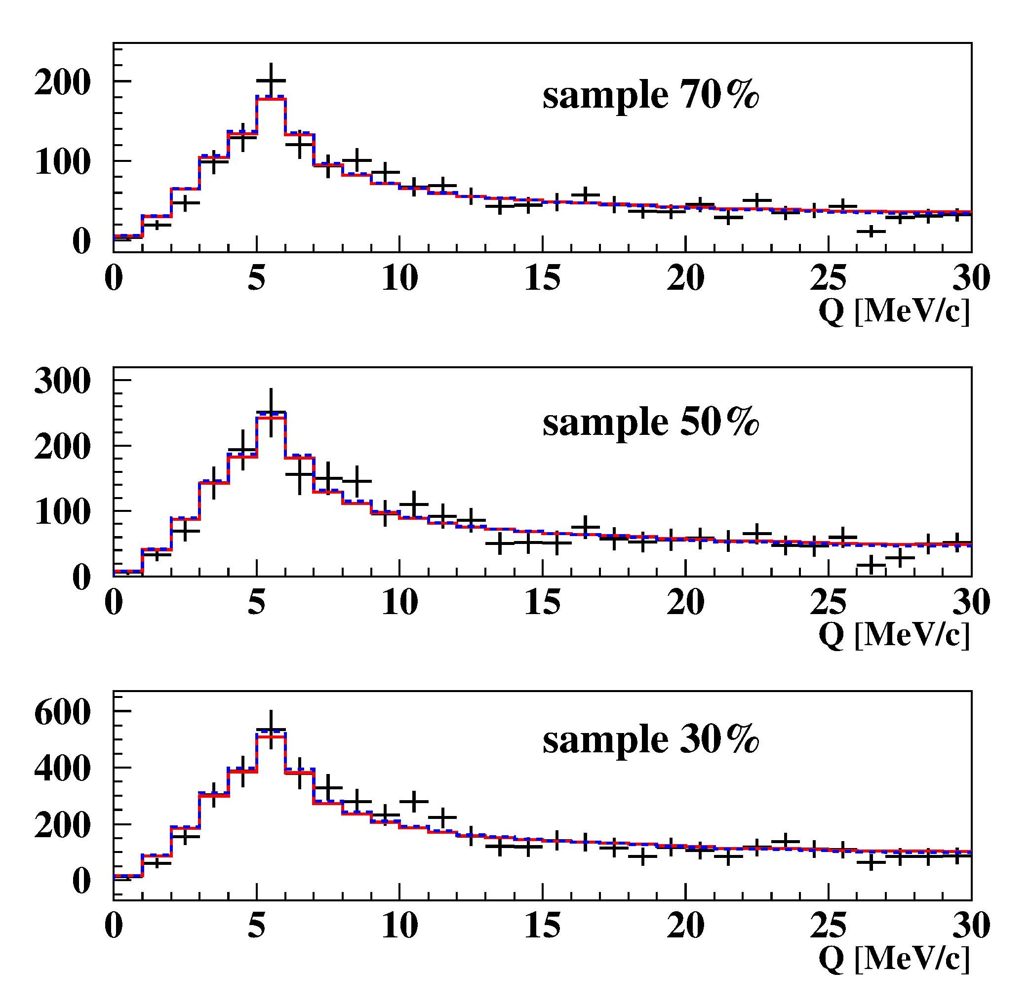
Figure 9: $Q$ distributions in the interval $0-30~{}MeV/c$ of $K^{+}K^{-}$ (ALICE parametrization) of the subsamples 30%, 50% and 70% for the DATA1 and DATA2 after residual background subtraction. The red and the blue fitting curves were evaluated from the analysis of experimental distributions with residual background in Coulomb and Martin parametrizations respectively. It is seen that in this interval of $Q$ the difference between these curves is absent and they describe ”pure” experimental $K^{+}K^{-}$ distributions well.

The experimental distributions after residual background subtraction using ALICE parametrization are shown in Figure 8 together with the fitting curves of Martin and point-like Coulomb parametrizations. The average background level in the corrected experimental distributions in the 70% and 30% subsamples are less than 3%. It is seen from the numbers of $K^{+}K^{-}$ pairs presented in Tables 3 and 4 that the point-like Coulomb parametrization is giving the yield of $K^{+}K^{-}$ pairs by 7%-8% (5%-6%) more than Martin (ALICE) parametrization in the $Q$ interval $0-100MeV/c$. The yields difference caused by strong $K^{+}K^{-}$ interaction in the final state is taken into account only in Martin (ALICE) parametrization. The distributions in the $Q$ interval $0-30MeV/c$ are presented in Figure 9. It is seen that Martin and Coulomb fitting curves describe well the corrected experimental data.

In Table 4 are presented the $K^{+}K^{-}$ pairs numbers for DATA1 and DATA2. Using the residual $R$ values from Table 2 were calculated the total number of $K^{+}K^{-}$ pairs with $Q_{t}<6MeV/c$, $0<Q<100MeV/c$ detected in the experiment. It is seen from Table 2 that the number of $K^{+}K^{-}$ pairs in the 3 subsamples for DATA1 and DATA2 are in agreement. The total number of detected $K^{+}K^{-}$ pairs evaluating from the most reliable 70% subsample is $40890\pm 4110$. The same values calculated with the 50% and 30% subsamples are $29650\pm 3880$ and $38140\pm 4430$ pairs respectively. The $K^{+}K^{-}$ pairs number in the 50% subsample differs from the two other values by about 3 standard deviations, confirming as mentioned above, that experimental data in this subsample is less reliable. The total number of $K^{+}K^{-}$ pairs calculated using the Martin parametrization from the ALICE parametrization values is significantly smaller than the presented errors.

The ratio of $K^{+}K^{-}$ pairs to the total number of subtracted background pairs in the 70% subsample case is 10 times larger than in the 30% subsample one. Nevertheless the total numbers of $K^{+}K^{-}$ pairs are in good agreement, demonstrating that the background and residual background subtractions were done correctly.

7 Conclusion

The DIRAC experiment at CERN detected in the reaction $\rm{p}(24~{}\rm{GeV}/c)+Ni$ the particle pairs $K^{+}K^{-},\pi^{+}\pi^{-}$ and $p\bar{p}$ with relative momentum $Q$ between $0-100~{}\rm{MeV}/c$. The $Q$ spectrum of $K^{+}K^{-}$ pairs was studied with the cut on the transverse component $Q_{T}<6~{}\rm{MeV}/c$. Three subsamples with $Q$ distributions of $K^{+}K^{-}$ pairs were obtained by subtracting background from initial experimental distributions with $K^{+}K^{-}$ populations larger than 70%, 50% and 30%. The $K^{+}K^{-}$ pair numbers, including residual background pairs, are 3790 (70%), 6420 (50%) and 11030 (30%).

These pair distributions in $Q$ and its longitudinal projection $Q_{L}$ were analyzed in two theoretical models. In the first model, only Coulomb FSI was taken into account, assuming point-like pair production. In the second more precise approach, three theoretical models were used, which consider Coulomb and strong FSI interactions via the resonances $f_{0}(980)$ and $a_{0}(980)$ and the dependence of these interactions in the distance $r^{*}$ between the produced $K$ mesons.

The analysis based on the first model showed, that the Coulomb FSI interaction increases the yield of $K^{+}K^{-}$ pairs about four times at $Q_{L}=0.5~{}\rm{MeV}/c$ compared to $100~{}\rm{MeV}/c$.

In the second approach, the $K^{+}K^{-}$ strong interaction was described using three parameter sets obtained in the Achasov, Martin and ALICE studies [41, 40, 38] by analyzing the experimental data sets. The numbers of $K^{+}K^{-}$ and residual background pairs were obtained using different $Q$ shapes of these pair distributions. In each subsample, the experimental spectrum was described as the sum of $K^{+}K^{-}$ and residual background distributions. It was shown, that the Coulomb model, ALICE and Martin parametrizations are describing the experimental distributions in the three subsamples well. The best description is provided by the set of ALICE parameters with the following number of $K^{+}K^{-}$ pairs: $3680\pm 370~{}(70\%),5040\pm 660~{}(50\%)$ and $10680\pm 1240~{}(30\%)$ with a background level of 3% for the 70% and 30% subsamples. The same numbers of $K^{+}K^{-}$ pairs, evaluated in the first model, are $3900\pm 410,5320\pm 730$ and $11220\pm 1370$, which differ from the corresponding ALICE values less than one error. The shape of the $K^{+}K^{-}$ spectrum in the $Q$ interval $0-30~{}\rm{MeV}/c$ is nearly the same in the ALICE, Martin and Coulomb parametrizations in all subsamples. Also the distribution of the distance $r^{*}$ between the produced kaons does not have a measurable effect on the $Q$ spectrum.

The experimental precision of the DIRAC data does not allow to choose between the simple Coulomb model and the more precise Martin and ALICE approaches, taking into account Coulomb and strong FSI, because all three models give practically the same $\chi^{2}$ and the levels of the residual background were evaluated correctly.

The total numbers of detected $K^{+}K^{-}$ pairs were evaluated in the ALICE parametrization using the known cuts on time-of-flight, which were used to suppress the background level. This number is $40890\pm 4110$ for the most reliable 70% subsample and $38140\pm 4430$ for the 30% subsample. The $K^{+}K^{-}$ pair number in the 50% subsample differs from the two other values by about three standard deviations, confirming – as mentioned above – that experimental data in this subsample is less reliable. The total $K^{+}K^{-}$ pair number calculated with the Martin parametrization deviates from the ALICE parametrization values less than the presented errors.

The ratio of $K^{+}K^{-}$ number to the total background level in the 70% subsample is 10 times larger than in the 30% subsample. Nevertheless, the total numbers of $K^{+}K^{-}$ pairs are in good agreement, demonstrating that the background and residual background subtractions were done correctly.

References

- [1] J. Uretsky and J. Palfrey, Phys. Rev. 121 (1961) 1798.
- [2] S.M. Bilenky et al., Yad. Phys. 10 (1969) 812, Sov. J. Nucl. Phys. 10 (1969) 469.
- [3] L. Nemenov, Yad. Fiz. 41 (1985) 980; Sov. J. Nucl. Phys. 41 (1985) 629.
- [4] L.G. Afanasyev and A.V. Tarasov, Yad. Fiz. 59 (1996) 2212; Phys. Atom. Nucl. 59 (1996) 2130.
- [5] L. Afanasyev et al., Phys. Lett. B 308 (1993) 200.
- [6] L. Afanasyev et al., Phys. Lett. B 338 (1994) 478.
- [7] B. Adeva et al., J. Phys. G: Nucl. Part. Phys. 30 (2004) 1929.
- [8] B. Adeva et al., Phys. Lett. B 619 (2005) 50.
- [9] B. Adeva et al., Phys. Lett. B 704 (2011) 24.
- [10] B. Adeva et al., Phys. Lett. B 751 (2015) 12.
- [11] B. Adeva et al., Phys. Lett. B 674 (2009) 11.
- [12] B. Adeva et al., Phys. Lett. B 735 (2014) 288.
- [13] B. Adeva et al., Phys. Rev. Lett. 117 (2016) 112001.
- [14] B. Adeva et al., Phys. Rev. D96 (2017) 052002.
- [15] R. Lednicky, J. Phys. G: Nucl. Part. Phys. 35 (2008) 125109.
- [16] R. Lednicky, Phys.Part.Nucl. 40 (2009) 307-352.
- [17] S.Wycech and A.M.Green Nucl.Phys. A562 (1993) 446.
- [18] G. Gamov, Z. Phys. 51 (1928) 204.
- [19] A. Sommerfeld, Atombau und Spektrallinien, F. Vieweg & Sohn (1931).
- [20] A.D. Sakharov, Sov. Phys. Usp. 34 (1991) 375.
- [21] S.Krewald, R.H.Lemmer, and F.P.Sassen, Phys.Rev. D 69,016003 (2004).
- [22] Yin-Jie Zhang et al., Phys.Rev. D74, 014013 (2006).
- [23] S.P.Klevansky, R.H.Lemmer, Phys.Lett. B 702(2011) 235.
- [24] C.Helmes et al., arXiv:1703.04737v2 [hep-lat] 24 Mar 2017.
- [25] L.R.Wiencke et al., Phys.Rev.D 46 (1992) 3708.
- [26] B. Adeva et al., Nucl. Instr. Meth. A 839 (2016) 52.
- [27] O. Gorchakov and A. Kuptsov, DN (DIRAC Note) 2005-05; cds.cern.ch/record/1369686.
- [28] O. Gorchakov, DN 2005-23; cds.cern.ch/record/1369668.
- [29] M. Pentia et al., Nucl. Instr. Meth. A 795 (2015) 200.
- [30] P.V. Chliapnikov, DIRAC-NOTE-2018-01.
- [31] P. Doskarova and V. Yazkov, DN 2013-05; cds.cern.ch/record/1628541.
- [32] DIRAC Collaboration, dirac.web.cern.ch/DIRAC/offlinedocs/Userguide.html.
- [33] R. Lednicky, T.B.Progulova, Z.Phys. C55 (1992) 295.
- [34] R. Lednicky, V.L. Lyuboshitz, Sov.J.Nucl.Phys. 35 (1982) 770.
- [35] S. Bekele and R. Lednicky, Braz.J.Phys. 37 (2007) 994; B.I. Abelev et al. (STAR Collaboration), Phys. Rev. C 74 (2006) 054902.
- [36] S.V. Afanasiev et al. (NA49 Collaboration), Phys. Lett. B 557 (2003) 157.
-
[37]
J. Lidrych for the STAR Collaboration.
indico.cern.ch/event/539093/contributions/2568038/attachments/
1476379/2287281/WPCF2017_KK_femto_Lidrych.pdf
- [38] K. Mikhailov for the ALICE Collaboration, J. Phys.: Conf. Ser. 1690 (2020) 012099.
- [39] B. Abelev et al. (ALICE Collaboration), Phys. Lett. B 717 (2012) 151; S. Acharya et al. (ALICE Collaboration), Phys. Rev. C 96 (2017) 064613.
- [40] A.D. Martin, E.N. Ozmutlu, and E.J. Squires, Nucl. Phys. B 121 (1977) 514 (1977).
- [41] N.N. Achasov, V.V. Gubin, Phys. Rev. D 63 (2001) 094007; N.N. Achasov, A.N. Kiselev, Phys. Rev. D 68 (2003) 014006.
- [42] A. Antonelli, hep-ex/0209069, eConf C020620 THAT06 (2002).
- [43] S. Acharya et al. (ALICE Collaboration), Phys. Lett. B 774 (2017) 64; Phys. Lett. B 790 (2019) 22.
- [44] A. Benelli, J. Smolik V. Yazkov, DN 2020-01; cds.cern.ch/record/2772989.